Dynamical histories of the IC 348 and NGC 1333 star-forming regions in Perseus

Abstract

We present analyses of the spatial distributions of stars in the young (1 – 3 Myr) star-forming regions IC 348 and NGC 1333 in the Perseus Giant Molecular Cloud. We quantify the spatial structure using the $\mathcal{Q}$-parameter and find that both IC 348 and NGC 1333 are smooth and centrally concentrated with $\mathcal{Q}$-parameters of 0.98 and 0.89 respectively. Neither region exhibits mass segregation ($\Lambda_{\rm MSR}=1.1^{+0.2}_{-0.3}$ for IC 348 and $\Lambda_{\rm MSR}=1.2^{+0.4}_{-0.3}$ for NGC 1333, where $\Lambda_{\rm MSR}\sim 1$ corresponds to no mass segregation), nor do the most massive stars reside in areas of enhanced stellar surface density compared to the average surface density, according to the $\Sigma_{\rm LDR}$ method.

We then constrain the dynamical histories and hence initial conditions of both regions by comparing the observed values to $N$-body simulations at appropriate ages. Stars in both regions likely formed with sub-virial velocities which contributed to merging of substructure and the formation of smooth clusters. The initial stellar densities were no higher than $\rho\sim 100-500$ M_⊙ pc^-3 for IC 348 and $\rho\sim 500-2000$ M_⊙ pc^-3 for NGC 1333. These initial densities, in particular that of NGC 1333, are high enough to facilitate dynamical interactions which would likely affect $\sim$10 per cent of protoplanetary discs and binary stars.

1 Introduction

Most stars form in regions where the local stellar density exceeds that of the Galactic field by several orders of magnitude (Porras et al., 2003; Lada & Lada, 2003; Bressert et al., 2010). However, it is currently unclear what fraction of stars are either born in, or experience, a dense stellar environment before they disperse into the field. If most star-forming regions are initially very dense (e.g.  $>$100 stars pc^-3), then dynamical encounters can alter or disrupt the orbits of binary stars (e.g. Kroupa, 1995; Marks et al., 2011; Parker & Goodwin, 2012) and planetary systems (e.g. Bonnell et al., 2001; Adams et al., 2006; Parker & Quanz, 2012). It is therefore crucial to determine the typical maximum density of star-forming regions before they dissolve into the Galactic disc.

An initially dense star-forming region will expand due to two-body relaxation (Gieles et al., 2012; Moeckel et al., 2012; Parker & Meyer, 2012) and so the observed present-day density may be much lower than the initial density. This degeneracy can be overcome by incorporating information on the spatial structure of the region. Stars form in filaments (André et al., 2014), and this results in a hierarchically substructured spatial distribution for the stars in some observed regions (Cartwright & Whitworth, 2004; Sánchez & Alfaro, 2009), and in hydrodynamical simulations of star formation (Bonnell et al., 2003; Bate, 2009; Dale & Bonnell, 2012; Dale et al., 2014).

In previous work, we have shown that combining the spatial structure with measures of the relative spatial distribution of the most massive stars, compared to low-mass stars, places constraints on the initial density and virial state of a region (Parker et al., 2014; Parker, 2014; Wright et al., 2014). Two-body relaxation erases primordial substructure and leads to the most massive stars residing in areas of relatively high local density (Parker et al., 2014), and violent relaxation can facilitate dynamical mass segregation on timescales commensurate with the ages of young star clusters (McMillan et al., 2007; Allison et al., 2010).

In order to determine the initial or maximum density of a star-forming region, a reasonably complete membership census is required, as well as mass determinations for all objects. Thus far, only four star-forming regions – the Orion Nebula Cluster, Taurus, $\rho$ Ophiuchus and Cyg OB2 – have had their initial densities constrained by this method. In this paper, we use the most recent censuses of the nearby ($<$350 pc), young (1 – 3 Myr) IC 348 and NGC 1333 star-forming regions in the Perseus Giant Molecular Cloud from Luhman et al. (2016) to determine the spatial structure and relative spatial distributions of the most massive stars compared to other stars and brown dwarfs.

The paper is organised as follows. In Section 2 we describe the datasets used, in Section 3 we outline the methods used to quantify the spatial distributions and in Section 4 we present the results for IC 348 and NGC 1333. We compare these results to $N$-body simulations of the evolution of star clusters to constrain the initial density of both regions in Section 5. We provide a discussion in Section 6 and we conclude in Section 7.

2 Datasets

For the observational sample, we adopted the most recent census of IC 348 and NGC 1333 clusters presented in Luhman et al. (2016), where tens of new low-mass stars and brown dwarf candidate members have been confirmed spectroscopically. Additionally, Luhman et al. (2016) have classified spectroscopically several previously known members, resulting in an unprecedented census with a number of members of 478 for IC 348 and 203 for NGC 1333. In both clusters, all members have measured magnitudes and an estimate of extinction, as well as a spectral type, except for 19 members of IC 348 and 41 members of NGC 1333.

To estimate the masses of the members of the clusters, we first converted spectral types to temperatures, adopting the temperature scale from Schmidt-Kaler (1982) for stars earlier than M0, and the scale from Luhman et al. (2003) for sources with spectral type between M0 and M9.5. For the L dwarfs, we applied the scale proposed by Lodieu et al. (2008). The bolometric luminosity was calculated by de-reddening the magnitudes of the targets with the extinction law from Rieke & Lebofsky (1985), using a distance to the clusters of 300 pc for IC 348 and 235 pc for NGC 1333, and bolometric corrections from Pecaut & Mamajek (2013), Herczeg & Hillenbrand (2015), and Dahn et al. (2002). Masses were derived from the evolutionary models (Baraffe et al., 1998; Chabrier et al., 2000; Siess et al., 2000) according to each target’s location on the HR diagram. For the lowest mass brown dwarfs (spectral types later than $\sim$M8), luminosities become more uncertain both in the data and the models, and therefore masses are derived only from temperatures using the models from Chabrier et al. (2000).

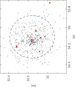
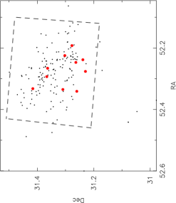
In Fig. 1 we show the positions of the objects in IC 348, and in Fig. 2 we show the positions of the objects in NGC 1333. In both plots the ten most massive stars in each region are shown by the large red points. Both regions have been extensively surveyed, and we show the areas that are observationally complete by the dashed lines. In IC 348 this corresponds to an area with radius 14’ from the central star BD +31 643 and in NGC 1333 the area covered by the Chandra X-ray Observatory Advanced CCD Imaging Spectrometer (ACIS-I). In addition to the full datasets, we will also perform our analyses only on objects within these areas.

Figure 1: Map of objects in IC348. The red points indicate the 10 most massive stars. The area within the dashed line is the 14’ radius from the centre which is observationally complete (Luhman et al., 2016).

Figure 2: Map of objects in NGC1333. The red points indicate the 10 most massive stars. The area within the dashed lines is the ACIS-I field from Luhman et al. (2016), which is observationally complete.

3 Methods

In this section we outline the techniques used to quantify the spatial distributions of stars and brown dwarfs in IC 348 and NGC 1333.

3.1 Spatial structure

We determine the amount of structure in a star forming region by measuring the $\mathcal{Q}$-parameter. The $\mathcal{Q}$-parameter was pioneered by Cartwright & Whitworth (2004); Bastian et al. (2009); Cartwright & Whitworth (2009); Cartwright (2009) and combines the normalised mean edge length of the minimum spanning tree (MST) of all the stars in the region, $\bar{m}$, with the normalised correlation length between all stars in the region, $\bar{s}$. The level of substructure is determined by the following equation:

$$\mathcal{Q}=\frac{\bar{m}}{\bar{s}}.$$ (1)

A substructured association or region has $\mathcal{Q}<0.8$, whereas a smooth, centrally concentrated cluster has $\mathcal{Q}>0.8$. The $\mathcal{Q}$-parameter has the advantage of being independent of the density of the star forming region, and purely measures the level of substructure present.

3.2 Mass segregation

In order to quantify the amount of mass segregation present in the clusters, we use the $\Lambda_{\rm MSR}$ method, introduced by Allison et al. (2009). This constructs a minimum spanning tree (MST) between a chosen subset of stars and then compares this MST to the average MST length of many random subsets.

We find the MST of the $N_{\rm MST}$ stars in the chosen subset and compare this to the MST of sets of $N_{\rm MST}$ random stars in the region. If the length of the MST of the chosen subset is shorter than the average length of the MSTs for the random stars then the subset has a more concentrated distribution and is said to be mass segregated. Conversely, if the MST length of the chosen subset is longer than the average MST length, then the subset has a less concentrated distribution, and is said to be inversely mass segregated (see e.g. Parker et al., 2011). Alternatively, if the MST length of the chosen subset is equal to the random MST length, we can conclude that no mass segregation is present.

By taking the ratio of the average (mean) random MST length to the subset MST length, a quantitative measure of the degree of mass segregation (normal or inverse) can be obtained. We first determine the subset MST length, $l_{\rm subset}$. We then determine the average length of sets of $N_{\rm MST}$ random stars each time, $\langle l_{\rm average}\rangle$. There is a dispersion associated with the average length of random MSTs, which is roughly Gaussian and can be quantified as the standard deviation of the lengths $\langle l_{\rm average}\rangle\pm\sigma_{\rm average}$. However, we conservatively estimate the lower (upper) uncertainty as the MST length which lies 1/6 (5/6) of the way through an ordered list of all the random lengths (corresponding to a 66 per cent deviation from the median value, $\langle l_{\rm average}\rangle$). This determination prevents a single outlying object from heavily influencing the uncertainty. We can now define the ‘mass segregation ratio’ ($\Lambda_{\rm MSR}$) as the ratio between the average random MST pathlength and that of a chosen subset, or mass range of objects:

$$\Lambda_{\rm MSR}={\frac{\langle l_{\rm average}\rangle}{l_{\rm subset}}}^{+{\sigma_{\rm 5/6}}/{l_{\rm subset}}}_{-{\sigma_{\rm 1/6}}/{l_{\rm subset}}}.$$ (2)

A $\Lambda_{\rm MSR}$ of $\sim$ 1 shows that the stars in the chosen subset are distributed in the same way as all the other stars, whereas $\Lambda_{\rm MSR}>1$ indicates mass segregation and $\Lambda_{\rm MSR}<1$ indicates inverse mass segregation, i.e.  the chosen subset is more sparsely distributed than the other stars.

There are several subtle variations of $\Lambda_{\rm MSR}$. Olczak, Spurzem & Henning (2011) propose using the geometric mean to reduce the spread in uncertainties, and Maschberger & Clarke (2011) and Delgado et al. (2013) propose using the median MST length to reduce the effects of outliers from influencing the results. However, in the subsequent analysis we will adopt the original $\Lambda_{\rm MSR}$ from Allison.

3.3 Relative local density

Maschberger & Clarke (2011) and Küpper et al. (2011) quantified the relative local density of a subset of objects with respect to the average local stellar density in the cluster. We calculate the local stellar surface density following the prescription of Casertano & Hut (1985), modified to account for the analysis in projection. For an individual star the local stellar surface density is given by

$$\Sigma=\frac{N-1}{\pi r_{N}^{2}},$$ (3)

where $r_{N}$ is the distance to the $N^{\rm th}$ nearest neighbouring star (we adopt $N=10$ throughout this work).

To determine whether a particular subset of stars, $\tilde{\Sigma}_{\mathrm{subset}}$, reside in areas of significantly higher than average density than the cluster average $\tilde{\Sigma}_{\mathrm{all}}$, we divide $\tilde{\Sigma}_{\mathrm{subset}}$ by $\tilde{\Sigma}_{\mathrm{all}}$ to define a ‘local density ratio’, $\Sigma_{\rm LDR}$:

$$\Sigma_{\rm LDR}=\frac{\tilde{\Sigma}_{\mathrm{subset}}}{\tilde{\Sigma}_{\mathrm{all}}}$$ (4)

The significance of this measure of the local density of a subset of stars compared to the cluster will be defined by a Kolmogorov-Smirnov (KS) test between the $\Sigma$ values of the subset against the $\Sigma$ values of the rest.

Parker et al. (2014) and Parker (2014) show that this can then be used to trace the initial density of a star-forming region because in very dense ($>$1000 stars pc^-3) regions, the most massive stars act as potential wells and collect retinues of low-mass stars, leading to $\Sigma_{\rm LDR}>>1$.

4 Results

4.1 IC 348

(a) $\Lambda_{\rm MSR}$, high mass

(b) $\Lambda_{\rm MSR}$, BDs

(c) $\Sigma-m$

Figure 3: Data for IC348. Panel (a) shows $\Lambda_{\rm MSR}$ as a function of the $N_{\rm MST}$ most massive stars. $\Lambda_{\rm MSR}=1.1$, which is probably not a significant deviation from unity. Panel (b) shows $\Lambda_{\rm MSR}$ as a function of the $N_{\rm MST}$ least massive objects. Again, the deviation from unity is not likely to be significant. Panel (c) shows the median surface density for the most massive stars (red line), cluster average (blue line) least massive BDs (orange line). Deviations from the median are not significant (KS test p-values of 0.49 and 0.20, respectively). The $\mathcal{Q}$-parameter is 0.98 (centrally concentrated).

4.1.1 Spatial structure

We apply the $\mathcal{Q}$-parameter to the IC 348 dataset and obtain $\mathcal{Q}=0.98$, which indicates a centrally concentrated distribution. Cartwright (2009) and Lomax et al. (2011) show that centrally concentrated morphologies can be sub-categorised by plotting the distribution of $\bar{m}$, the mean MST length, and $\bar{s}$, the mean separation length, although for complex morphologies this is highly non-trivial (Parker & Dale, 2015). In our data $\bar{m}=0.36$ and $\bar{s}=0.36$, which suggests a smooth, centrally concentrated density profile of the form $N\propto r^{-2.5}$. This is not as concentrated as a Plummer (1911) or King (1966) profile, suggesting a dynamically young cluster – we will examine this in more detail in the following Section 5.

Interestingly, Cartwright & Whitworth (2004) find $\mathcal{Q}=0.98$ for IC 348, with $\bar{m}=0.48$ and $\bar{s}=0.49$ for 288 objects from the Luhman et al. (2003) sample, which is also consistent with an $N\propto r^{-2.5}$ profile.

If we restrict our determination of the $\mathcal{Q}$-parameter to within the 14’ completeness radius from Luhman et al. (2016), we find $\mathcal{Q}=0.85$, with $\bar{m}=0.53$ and $\bar{s}=0.63$. This is a less centrally concentrated spatial profile ($N\propto r^{-1.5}$) than is measured for the full dataset; this is unsurprising as we are pruning the more distant objects from our determination of $\mathcal{Q}$.

4.1.2 Mass segregation ratio, $\Lambda_{\rm MSR}$

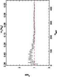
In Fig. 3(a) we show the evolution of $\Lambda_{\rm MSR}$ as a function of the $N_{\rm MST}$ most massive stars in the subset, which is compared to the MSTs of objects randomly drawn from the spatial distribution shown in Fig. 1. $\Lambda_{\rm MSR}=1.1^{+0.2}_{-0.3}$ for the $N_{\rm MST}=10$ most massive stars, and does not deviate from unity if we consider fewer (e.g.  $N_{\rm MST}=4$) or more stars.

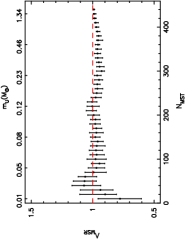
We then show the $\Lambda_{\rm MSR}$ ratio for the $N_{\rm MST}$ least massive objects (brown dwarfs) in Fig. 3(b). $\Lambda_{\rm MSR}=0.8^{+0.3}_{-0.1}$ for the $N_{\rm MST}=10$ least massive brown dwarfs and this plot suggests that these objects are not more or less spatially concentrated than the stars in IC 348.

We measure $\Lambda_{\rm MSR}\sim 1$ for the 14’ completeness field, suggesting that our results are not influenced by the inclusion or otherwise of outlying objects.

4.1.3 Local surface density ratio, $\Sigma_{\rm LDR}$

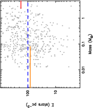
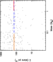
The local surface density as a function of mass is shown for all of the stars in our sample in Fig. 3(c). The median surface density for the whole star-forming region is shown by the blue dashed line, the median for the ten most massive stars is shown by the red line and the median surface density of the brown dwarfs is shown by the orange line. The surface density ratio for the most massive stars is $\Sigma_{\rm LDR}=1.77$, but a Kolmogorov-Smirnov (KS) test between the two populations gives $D=0.25$ and a $p-$value of 0.49 that the two populations share the same underlying parent distribution. Based on this, we cannot conclude that the most massive stars reside in areas of higher than average surface density.

If we compare the surface densities of brown dwarfs to the surface density of the whole star-forming region we have $\Sigma_{\rm LDR}=0.82$, which suggests the brown dwarfs reside in areas of lower than average surface density. However, the KS test between the two distributions has $D=0.33$ and the $p-$value is 0.20, again suggesting that the two populations share the same underlying distribution.

Previous studies have suggested that the most massive objects in IC 348 have significantly higher surface densities than the lowest mass objects (Kirk & Myers, 2012), and this gradient is also visually apparent in our dataset. The conclusion in Kirk & Myers (2012) was drawn from analysing a sample of 232 objects, which was split into two bins (high and low mass). This may introduce an inherent bias if one of the subsets in question (e.g.  the most massive stars) contains stars in regions of higher or lower density, because one is then not comparing a subset of objects to an ‘average’, such as the low-mass stars (0.08 – 1.0 M_⊙) in the sample.

We measure $\Sigma_{\rm LDR}=1.42$ for the objects within 14’ of the centre, and as for the full sample, the difference between the surface densities of the most massive stars compared to the whole region are not significant. We find similar conclusions when comparing the surface densities of the substellar objects to the whole region.

To summarise the results for IC 348, the star-forming region is centrally concentrated, with no evidence for mass segregation according to $\Lambda_{\rm MSR}$, but a suggestion that the most massive stars reside in areas of higher than average surface density.

4.2 NGC 1333

(a) $\Lambda_{\rm MSR}$, high mass

(b) $\Lambda_{\rm MSR}$, BDs

(c) $\Sigma-m$

Figure 4: Data for NGC1333. Panel (a) shows $\Lambda_{\rm MSR}$ as a function of the $N_{\rm MST}$ most massive stars. $\Lambda_{\rm MSR}=1.2$, which is probably not a significant deviation from unity. Panel (b) shows $\Lambda_{\rm MSR}$ as a function of the $N_{\rm MST}$ least massive objects. Again, the deviation from unity is not likely to be significant. Panel (c) shows the median surface density for the most massive stars (red line), cluster average (blue line) least massive BDs (orange line). Deviations from the median are not significant (KS test p-values of 0.92 and 0.22, respectively). The $\mathcal{Q}$-parameter is 0.89 (centrally concentrated).

4.2.1 Spatial structure

We obtain $\mathcal{Q}=0.89$, which also indicates a centrally concentrated distribution and $\bar{m}=0.33$ and $\bar{s}=0.37$. Due to the lower number of objects (162 compared to 459 for IC 348), placing constraints on the structure of NGC 1333 is more difficult, but like IC 348 it is consistent with a $N\propto r^{-2.5}$ profile.

If we restrict our determination of the $\mathcal{Q}$-parameter to within the ACIS-I completeness field, we find $\mathcal{Q}=0.79$, with $\bar{m}=0.50$ and $\bar{s}=0.64$. This is a less centrally concentrated spatial profile than is measured for the full dataset, and corresponds to a uniform distribution. Again, this is unsurprising as we are pruning the more distant objects from our determination of $\mathcal{Q}$.

4.2.2 Mass segregation ratio, $\Lambda_{\rm MSR}$

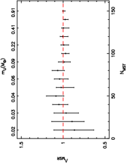
In Fig. 4(a) we show the evolution of $\Lambda_{\rm MSR}$ as a function of the $N_{\rm MST}$ most massive stars in the subset, which is compared to the MSTs of objects randomly drawn from the spatial distribution shown in Fig. 2. $\Lambda_{\rm MSR}=1.2^{+0.4}_{-0.3}$ for the $N_{\rm MST}=10$ most massive stars, and also does not deviate from unity if we consider fewer (e.g.  $N_{\rm MST}=4$) or more stars.

We then show the $\Lambda_{\rm MSR}$ ratio for the $N_{\rm MST}$ least massive objects (brown dwarfs) in Fig. 4(b). $\Lambda_{\rm MSR}=0.9^{+0.2}_{-0.3}$ for the $N_{\rm MST}=10$ least massive brown dwarfs and this plot suggests that these objects are not more or less spatially concentrated than the stars in IC 348.

$\Lambda_{\rm MSR}\sim 1$ for the ACIS-I completeness field, suggesting that our results are not influenced by the inclusion or otherwise of outlying objects.

4.2.3 Local surface density ratio, $\Sigma_{\rm LDR}$

The local surface density as a function of mass is shown for all of the stars in our sample in Fig. 4(c). The median surface density for the whole cluster is shown by the blue dashed line, the median for the ten most massive stars is shown by the red line and the median surface density of the brown dwarfs is shown by the orange line. The surface density ratio for the most massive stars is $\Sigma_{\rm LDR}=1.03$, and a KS test between the two populations gives $D=0.17$ and a $p-$value of 0.92 that the two populations share the same underlying parent distribution and we conclude that the most massive stars do not reside in more dense locations.

If we compare the surface densities of brown dwarfs to the surface density of the whole star-forming region we have $\Sigma_{\rm LDR}=1.00$, and the KS test between the two distributions gives $D=0.33$ and the $p-$value is 0.22, again suggesting that the two populations share the same underlying distribution.

$\Sigma_{\rm LDR}\sim 1$ for both the most massive stars and the substellar objects compared to all objects within the ACIS-I completeness field, suggesting that our results are not influenced by the inclusion or otherwise of outlying objects.

To summarise the results for NGC 1333, the star-forming region is centrally concentrated, with no evidence for mass segregation according to $\Lambda_{\rm MSR}$, and the most massive stars reside in areas of similar surface density to the average.

5 Comparison with $N$-body simulations

In order to place our values for $\mathcal{Q}$, $\Lambda_{\rm MSR}$ and $\Sigma_{\rm LDR}$ in context, we compare them to snapshots of $N$-body simulations of the evolution of star-forming regions. Parker et al. (2014) and Parker (2014) show that using combinations of $\mathcal{Q}$, $\Lambda_{\rm MSR}$ and $\Sigma_{\rm LDR}$ can place constraints on the initial virial ratio and the initial density of a star-forming region.

Both IC 348 and NGC 1333 have $\mathcal{Q}>0.8$, indicative of a smooth, centrally concentrated distribution with no substructure (Cartwright & Whitworth, 2004; Bastian et al., 2009; Sánchez & Alfaro, 2009). Because substructure is the expected outcome of star formation in filaments, we would expect dynamically pristine regions (i.e.  regions that have experienced little or no dynamical evolution) to have $\mathcal{Q}<<0.8$. This is corroborated by hydrodynamical simulations of star formation, which almost always display significant substructure (Bate, 2009; Girichidis et al., 2012; Dale et al., 2014; Parker et al., 2015). It is possible to ‘freeze in’ substructure if the initial virial state of the region is unbound, or if the region is in virial equilibrium but has a low stellar density (Parker et al., 2014).

Given that neither IC 348 nor NGC 1333 display substructure, we can deduce that they were initially subvirial or virialised, and so we will compare the observed datapoints to simulations of star-forming regions undergoing sub-virial collapse to form a cluster (Adams et al., 2006; Allison et al., 2010; Parker et al., 2014).

5.1 Simulation initial conditions

We tailor our $N$-body simulations to the observed star-forming regions by assigning masses from the complete samples for each region from Luhman et al. (2016), i.e.  the objects within the 14’ radius in IC 348 and the objects within the ACIS-I field in NGC 1333. This gives a total of 425 objects for our IC 348-like regions, and 150 objects for NGC 1333. We randomly assign masses to the objects in each simulation, meaning there is no preferred spatial distribution initially for any mass range. The mass functions for both regions are consistent with the Maschberger (2013) initial mass function (IMF), and in Appendix A we show how changing the mass function has little effect on the dynamical evolution of the regions.

The simulations are set up with primordial substructure, in an effort to mimic the initial conditions of star formation in both observed and (hydrodynamical) simulated star-forming regions. We create substructured regions using the fractal method, which is a (relatively) straightforward way of setting up substructure and we refer the interested reader to Goodwin & Whitworth (2004); Parker et al. (2014) for full details of the method. Observations (e.g. Larson, 1981; Hacar et al., 2013; André et al., 2014) suggest that stellar velocities are correlated on local scales at formation, and our fractal generator creates kinematic substructure as well as spatial substructure (see Parker & Wright, 2016, for details). The velocities of the stars are then scaled to the global virial ratio, $\alpha_{\rm vir}=0.3$, which makes the regions subvirial and induces collapse (Adams et al., 2006; Allison et al., 2010).

The degree of spatial and kinematic substructure is set by the fractal dimension, $D$, and our simulations all have $D=1.6$ initially (see Parker et al., 2014, for a full investigation of substructure parameter space). It is not straightforward to directly measure the fractal dimension of a star-forming region, and a proxy is usally used. We use the $\mathcal{Q}$-parameter (Cartwright & Whitworth, 2004; Cartwright, 2009; Lomax et al., 2011; Jaffa et al., 2017), which can be used to infer the fractal dimension of a region. However, the $\mathcal{Q}$-parameter is slightly dependent on the number of objects in a sample (Lomax et al., 2011; Parker & Dale, 2015), even though it is independent of the global size and density of a region. As an example, a highly substructured region ($D=1.6$) with 425 stars will have a lower $\mathcal{Q}$-parameter than a region with 150 stars, and this should be kept in mind when comparing star-forming regions with different numbers of objects (see e.g. Parker & Dale, 2015, their fig. 1 for an illustration of this).

We set up our simulations with a range of radii so as to vary the initial local stellar density. Depending on the simulation, this results in regions with initial densities as low as 10 M_⊙ pc^-3 to densities as high as 5000 M_⊙ pc^-3. A summary of the simulations, including their initial radii, stellar density and number of stars is given in Table 1.

Table 1: Summary of the $N$-body simulations used in this work. The columns show the star-forming region, mumber of stars, the IMF used (either the data from Luhman et al. (2016) or the Maschberger (2013) IMF), the radius of the star-forming region, $r_{F}$ and the median initial local density this radius results in, $\tilde{\rho}_{\rm ini}$.

Region	$N_{\rm stars}$	IMF	$r_{F}$	$\tilde{\rho}_{\rm ini}$
IC 348	425	Observed (Luhman et al., 2016)	0.5 pc	5000 – 10 000 M⊙ pc-3
IC 348	425	Observed (Luhman et al., 2016)	1.5 pc	100 – 500 M⊙ pc-3
IC 348	425	Maschberger (2013)	1.5 pc	100 – 500 M⊙ pc-3
IC 348	425	Observed (Luhman et al., 2016)	3 pc	10 – 60 M⊙ pc-3
NGC 1333	150	Observed (Luhman et al., 2016)	0.5 pc	500 – 2000 M⊙ pc-3
NGC 1333	150	Maschberger (2013)	0.5 pc	500 – 2000 M⊙ pc-3

(a) $\mathcal{Q}$-parameter

(b) $\mathcal{Q}-\Lambda_{\rm MSR}$

(c) $\mathcal{Q}-\Sigma_{\rm LDR}$

Figure 5: $N$-body simulations of star-forming regions containing 425 stars undergoing cool-collapse with stellar masses from the Luhman et al. (2016) sample for IC 348 and initial stellar densities of 5000 – 10 000 M_⊙ pc^-3. In panel (a) we show the evolution of the $\mathcal{Q}$-parameter; in panel (b) we show the $\mathcal{Q}-\Lambda_{\rm MSR}$ plot and in panel (c) we show the $\mathcal{Q}-\Sigma_{\rm LDR}$ plot. in panels (b) and (c) the simulation data at 0, 1 and 3 Myr are indicated by the plus signs, open circles and crosses, respectively. In all three panels, the blue diamond symbol shows the observational value at 3 Myr. The dashed horizontal line in all panels indicates the boundary between a substructured ($\mathcal{Q}<0.8$) and a smooth ($\mathcal{Q}>0.8$) distribution, and in panels (b) and (c) the vertical dashed lines indicate $\Lambda_{\rm MSR}=1$ (no mass segregation) and $\Sigma_{\rm LDR}=1$ (no enhanced surface densities) respectively.

(a) $\mathcal{Q}$-parameter

(b) $\mathcal{Q}-\Lambda_{\rm MSR}$

(c) $\mathcal{Q}-\Sigma_{\rm LDR}$

Figure 6: $N$-body simulations of star-forming regions containing 425 stars undergoing cool-collapse with stellar masses from the Luhman et al. (2016) sample for IC 348 and initial stellar densities of 100 – 500 M_⊙ pc^-3. In panel (a) we show the evolution of the $\mathcal{Q}$-parameter; in panel (b) we show the $\mathcal{Q}-\Lambda_{\rm MSR}$ plot and in panel (c) we show the $\mathcal{Q}-\Sigma_{\rm LDR}$ plot. in panels (b) and (c) the simulation data at 0, 1 and 3 Myr are indicated by the plus signs, open circles and crosses, respectively. In all three panels, the blue diamond symbol shows the observational values at 3 Myr. The dashed horizontal line in all panels indicates the boundary between a substructured ($\mathcal{Q}<0.8$) and a smooth ($\mathcal{Q}>0.8$) distribution, and in panels (b) and (c) the vertical dashed lines indicate $\Lambda_{\rm MSR}=1$ (no mass segregation) and $\Sigma_{\rm LDR}=1$ (no enhanced surface densities) respectively.

(a) $\mathcal{Q}$-parameter

(b) $\mathcal{Q}-\Lambda_{\rm MSR}$

(c) $\mathcal{Q}-\Sigma_{\rm LDR}$

Figure 7: $N$-body simulations of star-forming regions containing 425 stars undergoing cool-collapse with stellar masses from the Luhman et al. (2016) sample for IC 348 and initial stellar densities of 10 – 60 M_⊙ pc^-3. In panel (a) we show the evolution of the $\mathcal{Q}$-parameter; in panel (b) we show the $\mathcal{Q}-\Lambda_{\rm MSR}$ plot and in panel (c) we show the $\mathcal{Q}-\Sigma_{\rm LDR}$ plot. in panels (b) and (c) the simulation data at 0, 1 and 3 Myr are indicated by the plus signs, open circles and crosses, respectively. In all three panels, the blue diamond symbol shows the observational value at 3 Myr. The dashed horizontal line in all panels indicates the boundary between a substructured ($\mathcal{Q}<0.8$) and a smooth ($\mathcal{Q}>0.8$) distribution, and in panels (b) and (c) the vertical dashed lines indicate $\Lambda_{\rm MSR}=1$ (no mass segregation) and $\Sigma_{\rm LDR}=1$ (no enhanced surface densities) respectively.

(a) $\mathcal{Q}$-parameter

(b) $\mathcal{Q}-\Lambda_{\rm MSR}$

(c) $\mathcal{Q}-\Sigma_{\rm LDR}$

Figure 8: $N$-body simulations of star-forming regions containing 150 stars undergoing cool-collapse with stellar masses from the Luhman et al. (2016) sample for NGC 1333 and initial stellar densities of 500 – 2000 M_⊙ pc^-3. In panel (a) we show the evolution of the $\mathcal{Q}$-parameter; in panel (b) we show the $\mathcal{Q}-\Lambda_{\rm MSR}$ plot and in panel (c) we show the $\mathcal{Q}-\Sigma_{\rm LDR}$ plot. in panels (b) and (c) the simulation data at 0, 1 and 3 Myr are indicated by the plus signs, open circles and crosses, respectively. In all three panels, the blue hexagram symbol shows the observational value at 1 Myr. The dashed horizontal line in all panels indicates the boundary between a substructured ($\mathcal{Q}<0.8$) and a smooth ($\mathcal{Q}>0.8$) distribution, and in panels (b) and (c) the vertical dashed lines indicate $\Lambda_{\rm MSR}=1$ (no mass segregation) and $\Sigma_{\rm LDR}=1$ (no enhanced surface densities) respectively.

The simulations are evolved for 10 Myr using the kira integrator in the Starlab environment (Portegies Zwart et al., 1999, 2001). We do not include stellar evolution in the simulations as neither IC 348 or NGC 1333 contain stars massive enough to evolve significantly in the first 10 Myr.

5.2 Comparison with IC 348

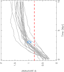
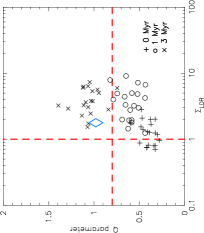
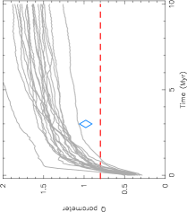
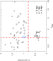
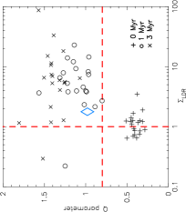
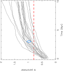
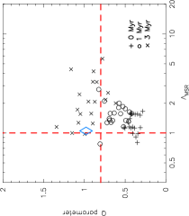
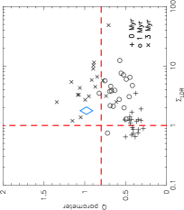
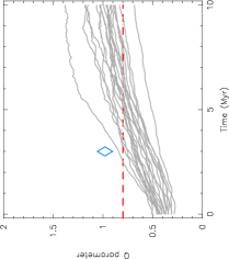
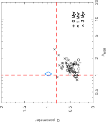
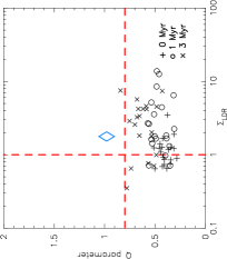
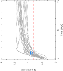
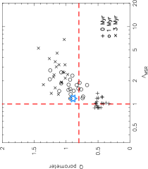
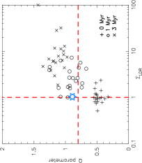
In Figs. 5, 6 and 7 we show the simulations set up to constrain the initial density of IC 348. In all three figures the blue diamond symbol corresponds to the observed value for IC 348 at its current age (3 Myr). In each figure, panel (a) shows the evolution of the $\mathcal{Q}$-parameter, panel (b) shows the $\mathcal{Q}$-parameter against the mass segregation ratio $\Lambda_{\rm MSR}$ at three epochs in the simulation (0, 1 and 3 Myr) and panel (c) shows the $\mathcal{Q}$-parameter against the local surface density ratio $\Sigma_{\rm LDR}$ at the same three epochs. The boundary between a substructured and a smooth distribution is indicated by the horizontal dashed line in all panels, and in panels (b) and (c) $\Lambda_{\rm MSR}=1$ (no mass segregation) and $\Sigma_{\rm LDR}=1$ (no enhanced surface densities) are shown by the vertical dashed lines.

We show the evolution of simulations with initial radii $r_{F}=0.5$ pc and 425 objects with masses from the Luhman et al. (2016) dataset assigned randomly with position in Fig. 5. Our fractal initial conditions with this radius gives an initial median stellar density between 5000 – 10 000 M_⊙ pc^-3, depending on the random number seed used to initialise the positions of the objects. These high stellar densities facilitate dynamical interactions, and the $\mathcal{Q}$-parameters in the simulations are higher at 3 Myr than the observed value because interactions erase substructure (Scally & Clarke, 2002; Goodwin & Whitworth, 2004; Parker & Meyer, 2012). Similarly, due to the high number of interactions, dynamical mass segregation often occurs (panel b), which is a natural outcome of dense, substructured and (sub)virial initial conditions (McMillan et al., 2007; Allison et al., 2010; Parker et al., 2014).

The massive stars also attain higher than average local densities (panel c) because they typically migrate to the centre of a subvirial, collapsing star-forming region (Parker et al., 2014), although other initial conditions can lead to high $\Sigma_{\rm LDR}$ values and for example the $\mathcal{Q}-\Sigma_{\rm LDR}$ plot (panel c) can used to distinguish between a dense, subvirial region (which would have high $\Sigma_{\rm LDR}$ and high $\Lambda_{\rm MSR}$) and a dense, supervirial ($\alpha_{\rm vir}=1.5$), whch would have high $\Sigma_{\rm LDR}$ but $\Lambda_{\rm MSR}\sim 1$. The evolution of a cluster with dense, subvirial initial conditions is to move up and to the right in both the $\mathcal{Q}-\Lambda_{\rm MSR}$ and $\mathcal{Q}-\Sigma_{\rm LDR}$ plots as it erases substructure, dynamically mass segregates and the massive stars attain higher than average local densities, all of which are inconsistent with the observed values (the blue diamonds).

In Fig. 6 we show the evolution of simulations with initial radii $r_{F}=1.5$ pc, 425 objects and masses assigned from the Luhman et al. (2016) sample, which gives initial stellar densities between 100 – 500 M_⊙ pc^-3. These stellar densities lead to a moderate level of dynamical evolution; substructure is erased within the first 1 – 5 Myr, and the simulations are consistent with the observed $\mathcal{Q}$-parameter at ages of 3 Myr (panel a). Around half of our simulations display mass segregation after 3 Myr, but several are consistent with the observed $\Lambda_{\rm MSR}$ value and $\mathcal{Q}$-parameter at these ages (the crosses in panel b). Similarly, several simulations present higher $\Sigma_{\rm LDR}$ values than are observed (panel c), but 25 per cent of the simulations are close to the observed $\mathcal{Q}-\Sigma_{\rm LDR}$ value on the plot.

In Fig. 7 we show the evolution of simulations with initial radii $r_{F}=3$ pc, 425 objects and masses assigned from the Luhman et al. (2016) sample, which gives initial stellar densities between 10 – 60 M_⊙ pc^-3. Spatial substructure is maintained due to these low densities, and the regions remain substructured until well after 5 Myr (panel a). No significant mass segregation occurs (panel b), but some simulations display high local surface densities for the most massive stars ($\Sigma_{\rm LDR}>>1$) after 3 Myr. However, because of the retention of substructure, $\mathcal{Q}<1$ and the $\mathcal{Q}-\Lambda_{\rm MSR}$ and $\mathcal{Q}-\Sigma_{\rm LDR}$ values are inconsistent with the observations.

In summary, our $N$-body simulations of IC 348 suggest the region was initially substructured and sub-virial or in virial equilibrium, with an initial stellar density in the range of 100 – 500 M_⊙ pc^-3.

5.3 Comparison with NGC 1333

We now focus on $N$-body simulations that attempt to mimic NGC 1333. We ran a series of models with different initial stellar densities, but for the sake of brevity we omit a discussion of the models whose initial density leads to dynamical evolution that is not consistent with the observations.

In Fig. 8 we show the evolution of simulations with initial radii $r_{F}=0.5$ pc, 150 objects and masses assigned from the Luhman et al. (2016) sample, which gives initial stellar densities between 500 – 2000 M_⊙ pc^-3. These relatively high stellar densities cause the erasure of substructure within the first 1 – 2 Myr, as shown by the evolution of the $\mathcal{Q}$-parameter in Fig. 8(a). However, the simulations rarely show evidence of mass segregation (panel b) or enhanced surface densities for the most massive stars (panel c) within the first 1 Myr. We find that simulations with much higher ($>$5000 M_⊙ pc^-3) or lower ($<$100 M_⊙ pc^-3) densities are inconsistent with the observations. The boundary between a substructured and a smooth distribution is indicated by the horizontal dashed line in all panels, and in panels (b) and (c) $\Lambda_{\rm MSR}=1$ (no mass segregation) and $\Sigma_{\rm LDR}=1$ (no enhanced surface densities) are shown by the vertical dashed lines. The blue hexagram symbols indicate the observed values for NGC 1333 assuming an age of 1 Myr.

The simulation values at 1 Myr are therefore consistent with the observed value for NGC 1333 if the region was initially substructured and sub-virial or in virial equilibrium, with an initial stellar density in the range of 500 – 2000 M_⊙ pc^-3.

6 Discussion

Our spatial analysis of IC 348 and NGC 1333 show that both star-forming regions are centrally concentrated, with no mass segregation and no enhanced surface densities for the most massive stars. The comparison with the $N$-body models suggest that IC 348 is consistent with having formed with some substructure, subvirial initial conditions and moderate stellar densities ($\tilde{\rho}\sim 100-500$ M_⊙ pc^-3). NGC 1333 is likely to have formed with slightly denser initial conditions ($\tilde{\rho}\sim 500-2000$ M_⊙ pc^-3).

6.1 Potential biases

In order to determine the structural diagnostics $\mathcal{Q}$, $\Lambda_{\rm MSR}$ and $\Sigma_{\rm LDR}$ in a region, we must first be confident of membership for each star (all three diagnostics), and secondly, reasonable estimates for individual stellar masses must be made ($\Lambda_{\rm MSR}$ and $\Sigma_{\rm LDR}$).

The datasets from Luhman et al. (2016) are the most complete censuses of NGC 1333 and IC 348 to date, and therefore the $\mathcal{Q}$-parameters are unlikely to be affected by incompleteness (Parker & Meyer, 2012; Parker & Dale, 2015). However, as we have shown, when we restrict our analyses to the regions that have been extensively surveyed (within the 14’ radius in IC 348 and the ACIS-I field in NGC 1333), the $\mathcal{Q}$-parameters are lower due to the pruning of more distant objects from the analysis. It is important to emphasise that if the areas outside the completeness limits are incomplete, and there is therefore more substructure in both regions, then each region is even more dynamically young, which reinforces our conclusion that they formed with moderate stellar densities. There is very little difference in the values of $\Lambda_{\rm MSR}$ and $\Sigma_{\rm LDR}$ within the completeness fields compared to the full datasets, which again suggests that our conclusions are robust against observational biases.

For $\Lambda_{\rm MSR}$ and $\Sigma_{\rm LDR}$, the individual stellar masses are likely accurate to within 20 – 30 per cent. This uncertainty on stellar mass in one sense is not important, as long as we correctly identify the subset of the ten most massive stars which are used to assess whether the region is mass segregated. Any stars hidden by differential extinction are likely to be lower mass, which would give the impression that the most massive stars are more centrally concentrated (i.e. $\Lambda_{\rm MSR}>1$), but have lower than average surface densities ($\Sigma_{\rm LDR}<1$). As we do not observe this combination, we can be resonably confident that our measurements are unaffected by this bias. As a check, we repeated our analyses excluding objects whose measured extinction exceeded $A_{V}>4$ magnitudes and found no difference to our results.

A caveat associated with the simulations is that our $N$-body models assume instantaneous star formation, which is obviously an idealised situation. The observations of Foster et al. (2015) show that star-forming cores seem to follow the gas structures on the outskirts of NGC 1333. It is therefore possible that the central regions of NGC 1333 (and indeed IC 348) will acquire more pre-main sequence stars over time as filaments merge (cf Bate, 2009; Myers, 2011). Our collapsing fractal simulations attempt to mimic this star-formation scenario, but fall short of modelling any of the gas physics. In this study $N$-body simulations do, however, hold the advantage in that they can be run to much older physical ages than hydrodynamical simulations, and can be directly compared to the observational data.

6.2 Comparison with kinematic studies

Recently, two separate studies have used high precision radial velocities to estimate the velocity dispersion of IC 348 and NGC 1333, and determined the dynamic state of each region by comparing the velocity dispersion with that expected if the region were in virial equilibrium using the virial mass estimate, $\sigma_{\rm vir}$, where

$$\sigma_{\rm vir}=\sqrt{\frac{2GM}{\eta R}}.$$ (5)

$M$ is the chosen mass enclosed within radius $R$, and $\eta$ depends on the density profile of the region in question, and is more difficult to determine.

Foster et al. (2015) observed a velocity dispersion in NGC 1333 of $\sigma=0.92\pm 0.12$ km s^-1, compared to a virial mass estimate of $\sigma_{\rm vir}=0.79\pm 0.20$ km s^-1, suggesting that the stars were in virial equilibrium. However, Foster et al. (2015) also determined the velocity dispersion for the pre-stellar cores, and determined that they were subvirial. They hypothesised that the prestellar cores form with subvirial velocities, and two-body and violent relaxation causes the forming stars to speed up and attain virial equilibrium (Parker & Wright, 2016).

Assuming that the prestellar cores observed today have similar kinematic properties to the pre-stellar cores that formed the present-day pre-main sequence stars, our data are consistent with this collapsing scenario for NGC 1333, especially given our conclusion that NGC 1333 was likely to have been more dense in the past.

In the case of IC 348, Cottaar et al. (2015) find it likely that this region is slightly supervirial, though still gravitationally bound. For very dense initial conditions ($\tilde{\rho}\sim 10^{4}$ M_⊙ pc^-3) the violent relaxation of initially subvirial clusters can create the illusion that they are supervirial and highly unbound following a cool-collapse (Parker & Wright, 2016). However, our analysis of the spatial diagnostics rules out such high initial stellar densities, suggesting that IC 348 either formed without substructure (i.e.  the present-day $\mathcal{Q}$-parameter reflects the initial conditions), or there may be an underlying problem with estimating the virial state from the velocity dispersion alone.

The scenario that IC 348 formed without primordial substructure is unlikely; even modest dynamical evolution in a star-forming region with a stellar density of $\sim 10^{2}$M_⊙ pc^-3 would result in the erasure of initial substructure (Scally & Clarke, 2002; Parker & Meyer, 2012; Parker & Dale, 2013; Parker et al., 2014; Parker, 2014) and the measured $\mathcal{Q}=0.98$ would result from dynamical evolution of a medium density region (as shown in Fig. 6(a)).

On the other hand, the use of the velocity dispersion in isolation to determine the virial state of a region was shown to be problematic by Parker & Wright (2016) for several reasons. First, the estimate of the velocity dispersion enclosed within the virial mass requires the determination of the structure parameter, $\eta$, which varies between $\sim 1-12$ depending on the amount of substructure present. Furthermore, the mass $M$ used to estimate the virial mass velocity dispersion in Equation 5 requires an estimate of the contribution of the gas potential, which is difficult to determine in IC 348 (Cottaar et al., 2015). Finally, the effects of binary orbital motion must first be removed from the velocity dispersion (Cottaar et al., 2012), which assumes the orbital properties of binaries in IC 348 are similar to binaries in the Solar neighbourhood. It is far from clear that binaries do have universal orbital properties in nearby star-forming regions (King et al., 2012; Parker, 2014).

6.3 A typical density for star formation?

It is worth placing the derived initial densities ($\tilde{\rho}\sim 100-500$ M_⊙ pc^-3 for IC 348 and $\tilde{\rho}\sim 500-2000$ M_⊙ pc^-3 for NGC 1333) in the context of those in other nearby star-forming regions. In Taurus, $\rho$ Ophiuchus and Chamaeleon I, the $\mathcal{Q}-\Sigma_{\rm LDR}$ diagram suggests initial densities very similar to their observed present-day density (Parker, 2014; Sacco et al., 2017). All three regions are low-mass (as are IC 348 and NGC 1333 and many other star-forming regions within 1 kpc of the Sun).

The Orion Nebula Cluster is the most massive nearby star-forming region, and its position on the $\mathcal{Q}-\Sigma_{\rm LDR}$ diagram points towards high-density ($\tilde{\rho}>10^{3}$ M_⊙ pc^-3) initial conditions. However, spatial and kinematic analysis of the more distant but massive Cyg OB2 association is also consistent with low-density initial conditions (Wright et al., 2014; Wright et al., 2016). A larger sample of star-forming regions should be analysed, but our results in tandem with others suggest that the typical stellar density of star formation is likely to be around $\tilde{\rho}\sim 10^{2}-10^{3}$M_⊙ pc^-3.

Interestingly, these stellar densities straddle the border between the density regime ($\tilde{\rho}>$1000 M_⊙ pc^-3) where dynamical interactions could significantly alter planetary systems and discs (Adams et al., 2006; Parker & Quanz, 2012; Vincke et al., 2015) and affect the orbital properties of binary systems (Kroupa, 1995; Parker & Goodwin, 2012) and much more benign initial conditions ($\tilde{\rho}\sim<$100 M_⊙ pc^-3) where dynamical interactions are unimportant. Clearly, a larger census of star-forming regions is required to address whether there exists a typical density for star formation, and kinematic data from Gaia (Gaia Collaboration et al., 2016) and associated spectroscopic surveys such as Gaia-ESO (Gilmore et al., 2012) will be crucial in our understanding of this problem.

7 Conclusions

We have presented an analysis of the spatial distributions of stars in two nearby star-forming regions in the Perseus molecular cloud, the 3 Myr old IC 348 and the 1 Myr old NGC 1333. We determine the structure as measured by the $\mathcal{Q}$-parameter, the $\Lambda_{\rm MSR}$ measure of mass segregation and the $\Sigma_{\rm LDR}$ measure of the relative surface densities of the most massive stars compared to low-mass stars. We then compare these values to $N$-body simulations of the evolution of star-forming regions with a range of initial conditions. Our conclusions are the following.

(i) IC 348 has a $\mathcal{Q}$-parameter of 0.98, $\Lambda_{\rm MSR}=1.1^{+0.2}_{-0.3}$ and $\Sigma_{\rm LDR}=1.77$. Compared to $N$-body simulations at similar ages (2 – 3 Myr), these values suggest subvirial, medium density ($\tilde{\rho}\sim 10^{2}$M_⊙ pc^-3) initial conditions.

(ii) Similarly, NGC 1333 has a $\mathcal{Q}$-parameter of 0.89, $\Lambda_{\rm MSR}=1.2^{+0.4}_{-0.3}$ and $\Sigma_{\rm LDR}=1.03$. Compared to $N$-body simulations at similar ages ($\sim$1 Myr), these values also suggest subvirial velocities, but with medium-to-high density ($\tilde{\rho}\sim 10^{3}$M_⊙ pc^-3) initial conditions.

(iii) The spatial analysis of NGC 1333 is consistent with estimates of its virial state using the radial velocity dispersion, whereas IC 348 is slightly discrepant in that the spatial analysis suggests the region is in virial equilibrium, whereas the velocity dispersion hints at a supervirial state.

(iv) The initial inferred density for IC 348 is similar to its present-day density ($\tilde{\rho}\sim 10^{2}$M_⊙ pc^-3), but is higher for NGC 1333. In comparison to other nearby star-forming regions, these initial densities are lower than that inferred for e.g.  the Orion Nebula Cluster, but higher than the nearby Taurus star-forming region.

Based on these results, and other nearby star-forming regions (Parker, 2014), the typical initial stellar density for star-forming regions is between $\tilde{\rho}\sim 10^{2}-10^{3}$ M_⊙ pc^-3, which is dense enough to perturb a moderate fraction (up to $\sim 10$ per cent; Parker & Quanz, 2012) of protoplanetary discs and binary stars.

Appendix A $N$-body simulations with a statistical IMF

The form of the initial mass function (IMF) is generally universal, at least on local scales (Bastian et al., 2010; Offner et al., 2014). Both IC 348 and NGC 1333 are consistent with the common analytical approximations for the form of the IMF in the literature (e.g. Kroupa et al., 1993; Chabrier, 2005; Maschberger, 2013). However, due to the low numbers of stars in each region (425 for IC 348 and 150 for NGC 1333), neither region has a fully sampled IMF and statistical variations can lead to noticeably different IMFs if they are randomly sampled (Elmegreen, 2006; Parker & Goodwin, 2007; Maschberger & Clarke, 2008).

Kouwenhoven et al. (2014) show that subtle changes to the IMF of a star cluster can lead to differences in the properties of the clusters at later ages and in this Section we examine the evolution of an IC 348-like star-forming region with masses drawn from a Maschberger (2013) IMF instead of using masses from the Luhman et al. (2016) datasets. We repeat the simulation from Section 5 with 425 stars and an initial radius of $r_{F}=1.5$ pc and draw masses from the probability distribution function in Maschberger (2013):

$$p(m)\propto\left(\frac{m}{\mu}\right)^{-\alpha}\left(1+\left(\frac{m}{\mu}\right)^{1-\alpha}\right)^{-\beta}.$$ (6)

Here, $\mu=0.2$ M_⊙ is the average stellar mass, $\alpha=2.3$ is the Salpeter (1955) power-law exponent for higher mass stars, and $\beta=1.4$ is used to describe the slope of the IMF for low-mass objects (which also deviates from the log-normal form; Bastian, Covey & Meyer, 2010). Finally, we sample from this IMF within the mass range $m_{\rm low}=0.01$ M_⊙ to $m_{\rm up}=50$ M_⊙.

The evolution of this star-forming region is shown in Fig. 9, which should be directly compared to Fig. 6. We also performed a similar experiment for an NGC 1333-like cluster, instead drawing 150 stars from Eqn. 6 and comparing with the evolution of the simulations in Fig. 8. The variation between the simulations for both regions is not beyond what we would expect in the stochastic evolution of low-mass systems (Allison et al., 2010; Parker et al., 2014) and we conclude that the mass function measured by Luhman et al. (2016) does not result in a different dynamical history from a similar region with a field-like IMF.

(a) $\mathcal{Q}$-parameter

(b) $\mathcal{Q}-\Lambda_{\rm MSR}$

(c) $\mathcal{Q}-\Sigma_{\rm LDR}$

Figure 9: As Fig. 6 but with stellar masses drawn randomly from an initial mass function. $N$-body simulations of star-forming regions containing 425 stars undergoing cool-collapse with stellar masses drawn from a Maschberger (2013) IMF and initial stellar densities of 100 – 500 M_⊙ pc^-3. In panel (a) we show the evolution of the $\mathcal{Q}$-parameter; in panel (b) we show the $\mathcal{Q}-\Lambda_{\rm MSR}$ plot and in panel (c) we show the $\mathcal{Q}-\Sigma_{\rm LDR}$ plot. in panels (b) and (c) the simulation data at 0, 1 and 3 Myr are indicated by the plus signs, open circles and crosses, respectively. In all three panels, the blue diamond symbol shows the observational value at 3 Myr.

References

- Adams et al. (2006) Adams F. C., Proszkow E. M., Fatuzzo M., Myers P. C., 2006, ApJ, 641, 504
- Allison et al. (2010) Allison R. J., Goodwin S. P., Parker R. J., Portegies Zwart S. F., de Grijs R., 2010, MNRAS, 407, 1098
- Allison et al. (2009) Allison R. J., Goodwin S. P., Parker R. J., Portegies Zwart S. F., de Grijs R., Kouwenhoven M. B. N., 2009, MNRAS, 395, 1449
- André et al. (2014) André P., Di Francesco J., Ward-Thompson D., Inutsuka S.-I., Pudritz R. E., Pineda J. E., 2014, Protostars and Planets VI, pp 27–51
- Baraffe et al. (1998) Baraffe I., Chabrier G., Allard F., Hauschildt P. H., 1998, A&A, 337, 403
- Bastian et al. (2010) Bastian N., Covey K. R., Meyer M. R., 2010, ARA&A, 48, 339
- Bastian et al. (2009) Bastian N., Gieles M., Ercolano B., Gutermuth R., 2009, MNRAS, 392, 868
- Bate (2009) Bate M. R., 2009, MNRAS, 392, 590
- Bonnell et al. (2003) Bonnell I. A., Bate M. R., Vine S. G., 2003, MNRAS, 343, 413
- Bonnell et al. (2001) Bonnell I. A., Smith K. W., Davies M. B., Horne K., 2001, MNRAS, 322, 859
- Bressert et al. (2010) Bressert E., Bastian N., Gutermuth R., Megeath S. T., Allen L., Evans, II N. J., Rebull L. M., Hatchell J., Johnstone D., Bourke T. L., Cieza L. A., Harvey P. M., Merin B., Ray T. P., Tothill N. F. H., 2010, MNRAS, 409, L54
- Cartwright (2009) Cartwright A., 2009, MNRAS, 400, 1427
- Cartwright & Whitworth (2004) Cartwright A., Whitworth A. P., 2004, MNRAS, 348, 589
- Cartwright & Whitworth (2009) Cartwright A., Whitworth A. P., 2009, MNRAS, 392, 341
- Casertano & Hut (1985) Casertano S., Hut P., 1985, ApJ, 298, 80
- Chabrier (2005) Chabrier G., 2005 Vol. 327 of Astrophysics and Space Science Library, The Initial Mass Function: from Salpeter 1955 to 2005. p. 41
- Chabrier et al. (2000) Chabrier G., Baraffe I., Allard F., Hauschildt P., 2000, ApJ, 542, 464
- Cottaar et al. (2015) Cottaar M., Covey K. R., Foster J. B., Meyer M. R., Tan J. C., Nidever D. L., Chojnowski S. D., da Rio N., Flaherty K. M., Frinchaboy P. M., Majewski S., Skrutskie M. F., Wilson J. C., Zasowski G., 2015, ApJ, 807, 27
- Cottaar et al. (2012) Cottaar M., Meyer M. R., Parker R. J., 2012, A&A, 547, A35
- Dahn et al. (2002) Dahn C. C., Harris H. C., Vrba F. J., Guetter H. H., Canzian B., Henden A. A., Levine S. E., Luginbuhl C. B., Monet A. K. B., Monet D. G., Pier J. R., Stone R. C., Walker R. L., Burgasser A. J., Gizis J. E., Kirkpatrick J. D., Liebert J., Reid I. N., 2002, AJ, 124, 1170
- Dale & Bonnell (2012) Dale J. E., Bonnell I. A., 2012, MNRAS, 422, 1352
- Dale et al. (2014) Dale J. E., Ngoumou J., Ercolano B., Bonnell I. A., 2014, MNRAS, 442, 694
- Delgado et al. (2013) Delgado A. J., Djupvik A. A., Costado M. T., Alfaro E. J., 2013, MNRAS, 435, 429
- Elmegreen (2006) Elmegreen B. G., 2006, ApJ, 648, 572
- Foster et al. (2015) Foster J. B., Cottaar M., Covey K. R., Arce H. G., Meyer M. R., Nidever D. L., Stassun K. G., Tan J. C., Chojnowski S. D., da Rio N., Flaherty K. M., Rebull L., Frinchaboy P. M., Majewski S. R., Skrutskie M., Wilson J. C., Zasowski G., 2015, ApJ, 799, 136
- Gaia Collaboration et al. (2016) Gaia Collaboration Brown A. G. A., Vallenari A., Prusti T., de Bruijne J. H. J., Mignard F., Drimmel R., Babusiaux C., Bailer-Jones C. A. L., Bastian U., et al. 2016, A&A, 595, A2
- Gieles et al. (2012) Gieles M., Moeckel N., Clarke C. J., 2012, MNRAS, 426, L11
- Gilmore et al. (2012) Gilmore G., Randich S., Asplund M., Binney J., Bonifacio P., Drew J., Feltzing S., Ferguson A., Jeffries R., Micela G., et al. 2012, The Messenger, 147, 25
- Girichidis et al. (2012) Girichidis P., Federrath C., Allison R., Banerjee R., Klessen R. S., 2012, MNRAS, 420, 3264
- Goodwin & Whitworth (2004) Goodwin S. P., Whitworth A. P., 2004, A&A, 413, 929
- Hacar et al. (2013) Hacar A., Tafalla M., Kauffmann J., Kovács A., 2013, A&A, 554, A55
- Herczeg & Hillenbrand (2015) Herczeg G. J., Hillenbrand L. A., 2015, ApJ, 808, 23
- Jaffa et al. (2017) Jaffa S. E., Whitworth A. P., Lomax O., 2017, MNRAS, 466, 1082
- King (1966) King I. R., 1966, AJ, 71, 64
- King et al. (2012) King R. R., Goodwin S. P., Parker R. J., Patience J., 2012, MNRAS, 427, 2636
- Kirk & Myers (2012) Kirk H., Myers P. C., 2012, ApJ, 745, 131
- Kouwenhoven et al. (2014) Kouwenhoven M. B. N., Goodwin S. P., de Grijs R., Rose M., Kim S. S., 2014, MNRAS, 445, 2256
- Kroupa (1995) Kroupa P., 1995, MNRAS, 277, 1491
- Kroupa et al. (1993) Kroupa P., Tout C. A., Gilmore G., 1993, MNRAS, 262, 545
- Küpper et al. (2011) Küpper A. H. W., Maschberger T., Kroupa P., Baumgardt H., 2011, MNRAS, 417, 2300
- Lada & Lada (2003) Lada C. J., Lada E. A., 2003, ARA&A, 41, 57
- Larson (1981) Larson R. B., 1981, MNRAS, 194, 809
- Lodieu et al. (2008) Lodieu N., Hambly N. C., Jameson R. F., Hodgkin S. T., 2008, MNRAS, 383, 1385
- Lomax et al. (2011) Lomax O., Whitworth A. P., Cartwright A., 2011, MNRAS, 412, 627
- Luhman et al. (2003) Luhman K. L., Briceño C., Stauffer J. R., Hartmann L., Barrado y Navascués D., Caldwell N., 2003, ApJ, 590, 348
- Luhman et al. (2016) Luhman K. L., Esplin T. L., Loutrel N. P., 2016, ApJ, 827, 52
- Luhman et al. (2003) Luhman K. L., Stauffer J. R., Muench A. A., Rieke G. H., Lada E. A., Bouvier J., Lada C. J., 2003, ApJ, 593, 1093
- Marks et al. (2011) Marks M., Kroupa P., Oh S., 2011, MNRAS, 417, 1684
- Maschberger (2013) Maschberger T., 2013, MNRAS, 429, 1725
- Maschberger & Clarke (2008) Maschberger T., Clarke C. J., 2008, MNRAS, 391, 711
- Maschberger & Clarke (2011) Maschberger T., Clarke C. J., 2011, MNRAS, 416, 541
- McMillan et al. (2007) McMillan S. L. W., Vesperini E., Portegies Zwart S. F., 2007, ApJL, 655, L45
- Moeckel et al. (2012) Moeckel N., Holland C., Clarke C. J., Bonnell I. A., 2012, MNRAS, 425, 450
- Myers (2011) Myers P. C., 2011, ApJ, 735, 82
- Offner et al. (2014) Offner S. S. R., Clark P. C., Hennebelle P., Bastian N., Bate M. R., Hopkins P. F., Moraux E., Whitworth A. P., 2014, Protostars and Planets VI, pp 53–75
- Olczak et al. (2011) Olczak C., Spurzem R., Henning T., 2011, A&A, 532, 119
- Parker (2014) Parker R. J., 2014, MNRAS, 445, 4037
- Parker et al. (2011) Parker R. J., Bouvier J., Goodwin S. P., Moraux E., Allison R. J., Guieu S., Güdel M., 2011, MNRAS, 412, 2489
- Parker & Dale (2013) Parker R. J., Dale J. E., 2013, MNRAS, 432, 986
- Parker & Dale (2015) Parker R. J., Dale J. E., 2015, MNRAS, 451, 3664
- Parker et al. (2015) Parker R. J., Dale J. E., Ercolano B., 2015, MNRAS, 446, 4278
- Parker & Goodwin (2007) Parker R. J., Goodwin S. P., 2007, MNRAS, 380, 1271
- Parker & Goodwin (2012) Parker R. J., Goodwin S. P., 2012, MNRAS, 424, 272
- Parker & Meyer (2012) Parker R. J., Meyer M. R., 2012, MNRAS, 427, 637
- Parker & Quanz (2012) Parker R. J., Quanz S. P., 2012, MNRAS, 419, 2448
- Parker & Wright (2016) Parker R. J., Wright N. J., 2016, MNRAS, 457, 3430
- Parker et al. (2014) Parker R. J., Wright N. J., Goodwin S. P., Meyer M. R., 2014, MNRAS, 438, 620
- Pecaut & Mamajek (2013) Pecaut M. J., Mamajek E. E., 2013, ApJS, 208, 9
- Plummer (1911) Plummer H. C., 1911, MNRAS, 71, 460
- Porras et al. (2003) Porras A., Christopher M., Allen L., Di Francesco J., Megeath S. T., Myers P. C., 2003, AJ, 126, 1916
- Portegies Zwart et al. (2001) Portegies Zwart S. F., McMillan S. L. W., Hut P., Makino J., 2001, MNRAS, 321, 199
- Portegies Zwart et al. (1999) Portegies Zwart S. F., Makino J., McMillan S. L. W., Hut P., 1999, A&A, 348, 117
- Rieke & Lebofsky (1985) Rieke G. H., Lebofsky M. J., 1985, ApJ, 288, 618
- Sacco et al. (2017) Sacco G. G., Spina L., Randich S., Palla F., Parker R. J., Jeffries R. D., Jackson R., Meyer M. R., Mapelli M., et al., 2017, A&A, in press (arXiv: 1701.03741)
- Salpeter (1955) Salpeter E. E., 1955, ApJ, 121, 161
- Sánchez & Alfaro (2009) Sánchez N., Alfaro E. J., 2009, ApJ, 696, 2086
- Scally & Clarke (2002) Scally A., Clarke C., 2002, MNRAS, 334, 156
- Schmidt-Kaler (1982) Schmidt-Kaler T., 1982, Bulletin d’Information du Centre de Donnees Stellaires, 23, 2
- Siess et al. (2000) Siess L., Dufour E., Forestini M., 2000, A&A, 358, 593
- Vincke et al. (2015) Vincke K., Breslau A., Pfalzner S., 2015, A&A, 577, A115
- Wright et al. (2016) Wright N. J., Bouy H., Drew J. E., Sarro L. M., Bertin E., Cuillandre J.-C., Barrado D., 2016, MNRAS, 460, 2593
- Wright et al. (2014) Wright N. J., Parker R. J., Goodwin S. P., Drake J. J., 2014, MNRAS, 438, 639
Appendix A -body simulations with a statistical IMF