Energy dissipation in sheared wet granular assemblies

Abstract

Energy dissipation in sheared dry and wet granulates is considered in the presence of an externally applied confining pressure. Discrete element simulations reveal that for sufficiently small confining pressures, the energy dissipation is dominated by the effects related to the presence of cohesive forces between the particles. The residual resistance against shear can be quantitatively explained by a combination of two effects arising in a wet granulate: i) enhanced friction at particle contacts in the presence of attractive capillary forces, and ii) energy dissipation due to the rupture and reformation of liquid bridges. Coulomb friction at grain contacts gives rise to an energy dissipation which grows linearly with increasing confining pressure, for both dry and wet granulates. Because of a lower Coulomb friction coefficient in the case of wet grains, as the confining pressure increases the energy dissipation for dry systems is faster than for wet ones.

I Introduction

The mechanics of wet granulates plays a prominent role in various fields of process engineering, including the production of pharmaceutics Faure et al. (2001); Leuenberger (2001); Paul and Sharma (1999); Komlev et al. (2002), wet granulation of powders Simons and Fairbrother (2000); Litster and Ennis (2004); Realpe and Velázquez (2008), sintering Shinagawa and Hirashima (1998) and food production B. Bhandari and Schuck (2013). Owing to this outstanding importance, a large number of experimental studies and physical models have been devoted to the mechanics of wet granular matter, e.g. Géminard et al. (1999); Fournier et al. (2005); Mitarai and Nori (2006); Scheel et al. (2008); Fiscina et al. (2012); Fall et al. (2014). The transport of stresses in a dry granulate is governed by an interplay between frictional and repulsive forces acting between the constituting grains. Dry granulates easily flow under external forces such as gravity and hardly resist to shear. However, a confining stress applied to the grains at the surface of the assembly can reversibly turn a dry granulate into a solid–like material Brown et al. (2010). Hence externally applied confining stresses alter the mechanics of a granular assembly. A change of the mechanical properties also occurs when dry grains are mixed with a small amount of a wetting liquid. Granular assembly then turns into a plastically deformable material, which can sustain finite tensile and shear stresses Halsey and Levine (1998).

In this paper, we explore the rheology of dry and wet granulates in the presence of an externally applied confining stress. To quantify the resistance to shear as a function of the confining stress, we determine the energy dissipated in an assembly of particles over a stationary shear cycle. We perform Discrete Element Simulations (DES) of dense granular packs with shearing protocol inspired by recent experiments of the 3D pack of wet and dry glass beads Herminghaus (2005); Fournier et al. (2005). Figure 1 shows a typical snapshot obtained using 3D tomography.

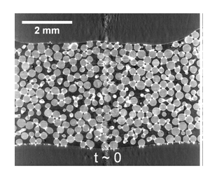
Figure 1: $2$D slice through a $3$D x-ray tomography of a sheared wet glass bead assembly Karmakar et al. , see also Fournier et al. (2005); Herminghaus (2005). The gray level indicates the different phases (white: aqueous $\rm ZnI_{2}$ solution; gray: glass beads; black air).

From the simulations, we extract the information about the source of energy dissipation due to direct particle-particle interaction (friction, inelastic interactions) as well as due to breaking and reformation of capillary bridges. The analysis of various contributions to the total energy dissipation provides an insight into the differences between dry and wet granular sheared packs and the main sources of energy loss. The main finding of our DES is that, for small applied pressures, the energy dissipated during the process of breakage and reformation of the capillary bridges is a main source of energy dissipation, dominating both the dissipation due to direct particle–particle interaction and the dissipation arising in the presence of capillary cohesion. However, for large applied pressure, friction dominates the particle–particle interaction for both wet and dry granulates. Accordingly, the work to shear a dry granulate becomes larger than that to shear a wet one for sufficiently large confining pressure.

This paper is organized as follows. In Section II we describe the setup of DES and discuss various energy loss mechanisms for wet and dry systems. In Section III we focus on energy dissipation mechanisms, discussing in particular the contributions due to non-affine motion of the particles and internal cohesion. We summarize the results in Section IV.

II Methods

II.1 Computational model

Discrete Element Simulations (DES) of two–dimensional packs of circular particles that are subject to shear deformations were carried out with a setup close to the experiments described in Fournier et al. (2005). The aim of this study is to reveal the fundamental mechanisms that control the dissipation in sheared assemblies of wet and dry particles. Details of the simulation techniques for dry granular matter could be found in e.g. Ref. Kovalcinova et al. (2015) and Appendix A. For later convenience we express all the quantities used in simulations in terms of the following scales: average particle diameter, $\bar{d}$, as the length–scale, average particle mass, $m$, as mass scale, and the binary particle collision time, $\tau_{\rm c}=\pi\sqrt{\bar{d}/2gk_{\rm n}}$, as the time scale. The parameter $k_{\rm n}$ corresponds to the normal spring constant between two colliding particles and $g$ is the acceleration of gravity. The parameters entering the force model can be connected to physical properties (Young modulus, Poisson ratio) as described, e.g. in Ref. Kondic (1999). The inter–particle friction coefficient for dry and wet assemblies is $\mu_{\rm dry}=0.29$ and $\mu_{\rm wet}=0.25$, respectively, to capture different friction properties of the granular material when a small amount of liquid is added between particles Fournier et al. (2005). Furthermore, we use $k_{\rm n}=4\times 10^{3}$, and the coefficient of restitution, as a measure of the inelasticity of collisions, is $e=0.5$.

The motivation for choosing the value of $k_{\rm n}$ that is smaller than appropriate for the glass beads used in the experiments Fournier et al. (2005) is the computational complexity: the simulations need to be carried out for long times in physical units, increasing computational cost; the use of softer particles allows for the use of larger computational time steps. To confirm that only quantitative features of the results are influenced by this choice, we have carried out limited simulations with stiffer particles, that led to similar results as the ones presented here.

In modeling capillary cohesion, we are motivated by the experiments Karmakar et al. , see also Fig. 1, and employ the capillary force model for three dimensional (3D) pendular bridges proposed by Willet et al. Willett et al. (2000). We motivate the choice of the force model between 3D spheres by the effort to use the same type of cohesive interaction between particles as the one expected in experiments. Note that according to Urso et al. (1999), cohesive force in 2D assumes a local maximum at a non-zero distance of the particles, in contrast to the 3D model. Furthermore, to simplify the implementation, we use the approximate expression, Eq. (12) in Willett et al. (2000); Herminghaus (2005), given here in nondimensional form

$$F_{\rm c,ij}={\frac{\pi d\sigma\cos\theta}{1+1.05\hat{S}_{\rm i,j}+2.5\hat{S}^{2}_{\rm i,j}}}\,,$$ (1)

where $\hat{S}_{\rm i,j}=S_{\rm i,j}\sqrt{1/(2V)}$ and $S_{\rm i,j}=r_{\rm i,j}-(d_{\rm i}+d_{\rm j})/2$ is the separation of the particle surfaces, where $r_{\rm i,j}$ is the distance between the centers of the circular particles $i,~{}j$. The inverse value of the reduced diameter is ${1/d}=({1/d_{\rm i}}+{1/d_{\rm j}})/2$ and $d_{\rm i},~{}d_{\rm j}$ are the particle diameters. The maximum separation, $S^{\rm max}$, at which a capillary bridge breaks is given by Willett et al. (2000):

$$S^{\rm max}=(2+{\theta})\left(\frac{V^{1/3}}{d}+\frac{2V^{2/3}}{d^{2}}\right)\,,$$ (2)

where $V$ is the non–dimensional capillary bridge volume. During a collision we set $S_{\rm i,j}=0.0$ (even when $r_{\rm i,j}<(d_{\rm i}+d_{\rm j})/2$) since the cohesive force has a constant value when the particles are in contact (regardless of the amount of compression resulting from collision) Herminghaus (2005).

For the contact angle, $\theta$, and the surface tension, $\sigma={\bar{\sigma}\tau_{\rm c}^{2}/m}$, we use $\theta=12^{\circ}$ and $\bar{\sigma}=72$ mN/m motivated by the parameters of the experiments in Fournier et al. (2005). The mass is computed from the density of a glass bead ($\rho=2.5\cdot 10^{3}$ kg/m³) of average diameter $\bar{d}$.

All capillary bridges in expressions (1) and (2) are assumed to have equal liquid volume $\bar{V}=7.4\cdot 10^{-3}\,\bar{d}^{3}$. This value corresponds to the average value in a 3D pack of monodisperse spherical beads with average diameter $\bar{d}$ with a liquid content of $W=2.5\%$ Herminghaus (2005) with respect to the total volume.

A bridge forms after two particles touch and breaks when the bridge length exceeds the maximum surface–to–surface separation $S^{\rm max}$. The energy dissipated during a full cycle of formation and rupture is computed by integrating the bridge force $F_{\rm c}$ between $S=0$ and $S=S^{\rm max}$, and can be expressed in closed form as:

$$E_{\rm c}^{\rm i,j} = 4\pi\sigma\cos\theta\,\sqrt{\frac{dV}{2\epsilon}}\Biggl{[}\arctan\biggl{(}5\bar{S}\sqrt{\frac{d}{2V\epsilon}}+\frac{\delta}{\sqrt{\epsilon}}\biggr{)}$$ (3)

$$- \arctan\biggl{\{}\frac{\delta}{\sqrt{\epsilon}}\biggr{\}}\Biggr{]},$$

with numerical constants $\delta=1.05$ and $\epsilon=8.8795$.

II.2 Simulation protocol

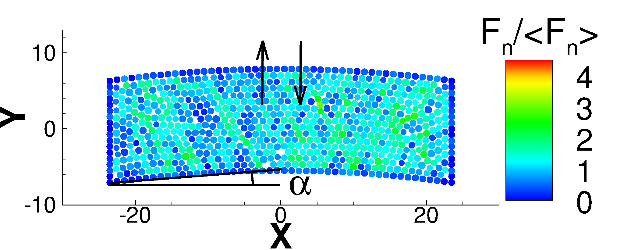
Figure 2: Snapshot of a granular domain with the particles colored according to the total normal force normalized by the average normal force imposed on the particles. The arrows show the upward and downward direction of the shear. For animation, see sup .

The simulation protocol is set up in such a way that closely follows the experimental one Herminghaus (2005); Fournier et al. (2005); Karmakar et al. . Figure 2 shows the example of a granular system during the shear. The simulation domain is initially rectangular and of the size $L_{\rm x},~{}L_{\rm y}$, with $L_{\rm x}=47$, and $L_{\rm y}=17$, both in units of $\bar{d}$. The walls are composed of monodisperse particles of size $\bar{d}$ and mass $m$. The system particles are chosen randomly from a uniform distribution with mean $\bar{d}$ and width $0.4\bar{d}$. Initially, the particles are placed on a rectangular grid and initialized with random velocities. Then, the top and bottom walls are moved inward by applying initial external pressure, $P_{\rm init}$, until equilibrium is reached and the position of the top and bottom wall stays fixed. At this point, we start shearing the system by prescribing a parabolic wall shape evolving in time. The maximum value of the shearing angle, $\alpha_{m}$, defined as the angle between the line connecting the endpoints of the left and right walls and the center of the bottom wall (see Fig. 2), is $\alpha_{m}=4^{\circ}$. The motion of the top/bottom wall is periodic in time with period $T$. At the beginning of a cycle, the system is sheared from the flat state ($\alpha=0$) in the positive vertical direction. After reaching $\alpha_{m}$, the shear continues in the opposite (negative) direction, until $\alpha$ reaches the value $-\alpha_{m}$ and the direction of the shear is reversed. The cycle is complete when the system reaches $\alpha=0$. More precisely, the motion of the top/bottom wall over time is given by

$$y(t) = \tan(\alpha_{m}){L_{\rm x}\over 2}\biggl{[}1-\biggl{(}{2x\over L_{\rm x}}\biggr{)}^{2}\biggr{]}v(t)+C$$ (4)

where $x$ is the position of the wall particle with respect to the horizontal axis (assuming that $x=0$ for the center of the top/bottom wall) and $v(t)=\gamma L_{\rm x}$; the shear rate $\gamma=10^{-4}\pi\cos(2\pi t/T)/(2L_{\rm x})\approx 10^{-6}$. The constant $C$ assumes the appropriate value for the top and bottom wall particles.

We let the top wall slide up and down to readjust the pressure until the system reaches a stationary shear cycle. Then, we fix the end points of both walls and continue shearing until the pressure inside of the system (found from Cauchy stress tensor), averaged over a shear cycle, reaches a constant value. The animation is available as supplementary material sup .

In the discussion that follows, we will use the average value of the pressure on top and bottom wall exerted by the system particles, $P_{1}$ and $P_{2}$, respectively, to define the confining pressure, $P_{\rm cf}=(P_{1}+P_{2})/2$.

II.3 Energies in Sheared Granular Assembly

Here we discuss the energy balance during shear, considering in detail energy input, dissipation, and balance.

II.3.1 Energy Input

During shear, the top and bottom walls have a prescribed parabolic shape that changes over time, and left and right boundaries are fixed. To compute the energy that is added to the system by moving the walls, one has to integrate the force over the boundary. There is no energy added to the system through the (fixed) left and right wall and we only need to find the energy entering through the collision of system particles with the top and bottom wall. This energy is given by

$$E_{\rm w}=\sum_{\rm j}\boldsymbol{F}_{\rm j}\cdot\boldsymbol{n}_{\rm j}ds\,,$$ (5)

where $j$ sums over all collisions of the bottom and top wall particles with any of the system particles. Here, $\boldsymbol{n}_{\rm j}$ is the unit vector normal to the boundary at the location of the wall particle experiencing a collision, ${\bf F}_{\rm j}$ is the force on the wall particle and $ds$ is the length element (here the wall particle diameter).

For the direction normal to the boundary at the center of the particle $w_{\rm j}$, we have $\boldsymbol{n}_{\rm j}\cdot\boldsymbol{t}_{\rm j}=0$ with $\boldsymbol{t}_{\rm j}$ being a unit vector tangential to the boundary at $w_{\rm j}$. The slope of the curve with the tangent vector $\boldsymbol{t}_{\rm j}$ is given by $y|_{x=x_{\rm j}}=2ax_{\rm j}$, where the value of $a$ is obtained from $y(t)$ and $x=x_{\rm j}$ in Eq. (4). Thus $\boldsymbol{t}_{\rm j}=(\boldsymbol{e}_{\rm x}+2ax_{\rm j}\boldsymbol{e}_{\rm y})/(1+4a^{2}x_{\rm j}^{2})^{1/2}$ and the unit normal vector $\boldsymbol{n}_{\rm j}$ is given by

$$\boldsymbol{n}_{\rm j}=\frac{(-2ax_{\rm j}\boldsymbol{e}_{\rm x}+\boldsymbol{e}_{\rm y})}{\sqrt{1+4a^{2}x_{\rm j}^{2}}}$$ (6)

Finally, from Eq. (5) and Eq. (6) we obtain the expression for the total energy added to the system by the moving walls

$$E_{\rm w} = \sum_{\rm j}\frac{(-2ax_{\rm j}\boldsymbol{e}_{\rm x}+\boldsymbol{e}_{\rm y})}{\sqrt{1+4a^{2}x_{\rm j}^{2}}}\cdot\boldsymbol{F}_{\rm j}ds\,.$$ (7)

II.3.2 Calculations of the Relevant Energy Contributions

Total energy stored in capillary bridge(s) between the particles $i,j$, can be found by integrating the force between them over the separating distance $S$ (smaller than the maximum separating distance $S^{\rm max}$)

$$E_{\rm c}^{\rm i,j}=\int_{0}^{\rm S}|\boldsymbol{F}_{\rm c,ij}|dS$$ (8)

with the functional form of $|\boldsymbol{F}_{\rm c,ij}|$ given in Eq. (1) with the closed form of the energy stored in a capillary bridge given in Eq. (3). The total energy stored in all capillary bridges is

$$E_{\rm c}=\sum_{\rm i,j}E_{\rm c}^{\rm i,j}\,,$$ (9)

for all pairs of particles $i,j$ that interact via capillary force.

Kinetic energy is computed as

$$E_{\rm k}=\sum_{\rm i=1}^{\rm N}\frac{m_{\rm i}|\boldsymbol{v}_{\rm i}|^{2}}{2}\,,$$ (10)

where $N$ is the total number of system particles and $m_{\rm i},~{}|\boldsymbol{v}_{\rm i}|$ are the mass and velocity of the $i$–th particle, respectively.

Elastic energy is computed as

$$E_{\rm el}=\sum_{\rm i,j}\frac{k_{\rm n}x_{\rm i,j}^{2}}{2}\,,$$ (11)

where $i,j$ runs over all pairs of overlapping particles, including the system particle – wall particle interactions.

II.3.3 Energy Balance

Energy dissipated due to rupturing of capillary bridges is equal to the capillary energy at the maximum separating distance $S^{\rm max}$. To find the total energy dissipated due to breaking and reformation of the bridges, we sum over all ruptured bridges

$$E_{\rm bb} = \sum_{\rm i,j}\int_{0}^{S^{\rm max}}|\boldsymbol{F}_{\rm c,ij}|dS\,.$$ (12)

The indices $i,j$ refer to all pairs of particles that experienced bridge rupturing.

Total energy dissipated during a time step can be computed from the energy balance equation described next. The energy entering the system due to the moving walls has to be equal to the sum of the changes in the elastic, kinetic and capillary energies, $\Delta E_{\rm el}(t),\Delta E_{\rm k}(t)$ and $\Delta E_{\rm b}(t)$, between two consecutive time steps, $(t-\Delta t)$ and $t$, the energy dissipated by breaking and reformation of capillary bridges $E_{\rm bb}(t)$ and the energy dissipated due to friction and other non–linear effects, $E_{\rm l}(t)$. The balance equation takes the form

$$E_{\rm w}(t)=\Delta E_{\rm el}(t)+\Delta E_{\rm k}(t)+\Delta E_{\rm c}(t)+E_{\rm l}(t)+E_{\rm bb}(t)\,.$$ (13)

From Eq. (13), we can compute the dissipated energy, $E_{\rm diss}(t)=E_{\rm l}+E_{\rm bb}$. For the dry systems we can use the same equation to find $E_{\rm diss}$ – there is no cohesion in the system and $E_{\rm c},~{}E_{\rm bb}=0$ trivially. Note that we ignore the energy dissipation due to viscous effects, as appropriate for the slow shear rates considered Herminghaus (2005); Karmakar et al. .

III Results

III.0.1 Pressure Evolution

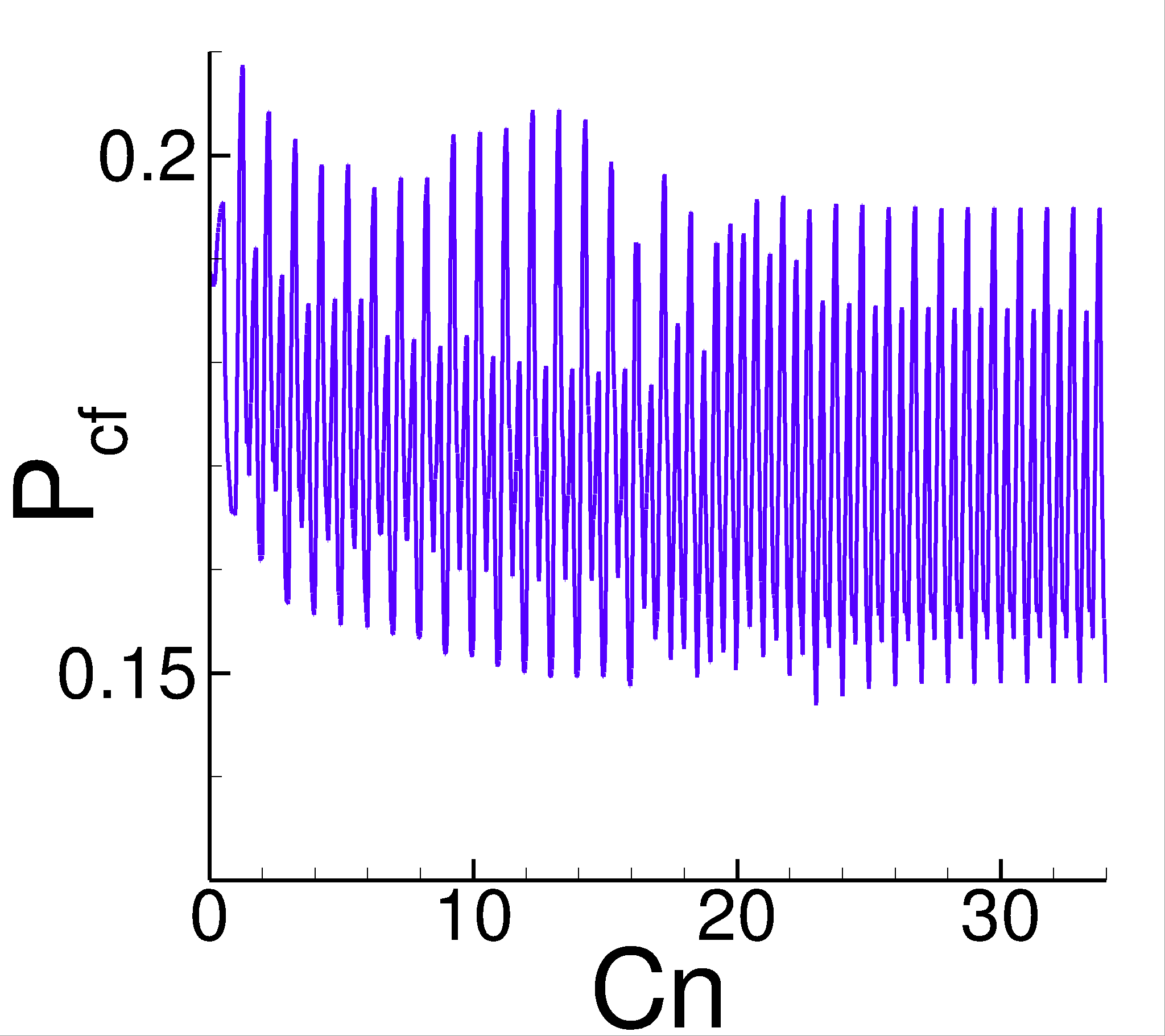
Figure 3: Evolution of the average confining pressure, $P_{\rm cf}$, over the cycles (denoted by $C_{\rm n}$) for wet system for the initial pressure $P_{\rm init}\approx 0.2$.

Figure 3 shows the average pressure on the top and bottom wall, $P_{\rm cf}$, for the wet systems with $P_{\rm init}\approx 0.2$. As already mentioned in Sec. II, $P_{\rm cf}$ evolves during first couple of shear cycles and finally reaches a stable behavior after $C_{\rm n}\approx 20$. Therefore the data used to draw our conclusions presented in this section are collected only after $P_{\rm cf}$ stabilizes. Note that the number of cycles needed to achieve stable $P_{\rm cf}$ behavior differs for each value of $P_{\rm init}$ and we average the results over last $15$ (stable) cycles.

As a side note, we comment that Fig. 3 shows that pressure evolution is not symmetric during a cycle, even when a stable regime is reached: the peak in $P_{\rm cf}$ that occurs when the system is sheared up towards $\alpha_{\rm m}$ is larger than the peak in $P_{\rm cf}$ when the system is sheared down towards $-\alpha_{\rm m}$. This asymmetry is observed for all different $P_{\rm init}$ and is due to the fact that we start shearing towards $\alpha_{\rm m}$ initially. We verified that shearing initially in the opposite direction reverses the asymmetry. While the influence of the initial conditions is not the focus of this paper, an existence of such a long-time memory of the system appears as a topic that requires further research.

III.0.2 Energy Transfer

Equation (13) allows to compute the energy dissipation for both wet and dry particles. Figure 4 shows the total dissipated energy, $E_{\rm diss}=E_{\rm l}+E_{\rm bb}$ (recall that in the dry case $E_{\rm bb}$ is trivially zero), averaged over $15$ stationary shear cycles, for both wet and dry assemblies. We note that the simulations, as implemented, are limited in the range of pressures that can be considered. For $P_{\rm cf}\lessapprox 0.06$ it is difficult to carry out simulations since the particles may detach from the walls. For pressures larger than $P_{\rm cf}\gtrapprox 0.3$, the overlap between the particles becomes large, suggesting that a different interaction model may be needed there.

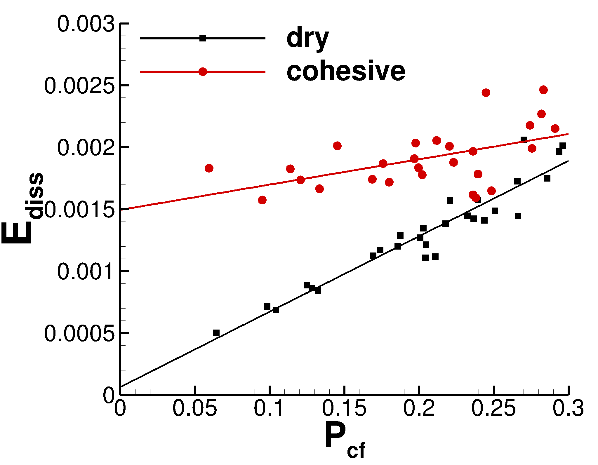
Figure 4: Dissipated energy during shear as a function of the confining pressure for dry (black squares) and wet particles (red circles). The results are averaged over 15 cycles. For the wet system, $E_{\rm diss}=E_{\rm l}+E_{\rm bb}$, see Eq. (13).

Figure 4 shows that the energy dissipated by friction increases with the confining pressure, $P_{\rm cf}$, in a manner which is consistent with linear behavior (although the scatter of data is significant, particularly for the wet systems). The increase of dissipated energy with $P_{\rm cf}$ is steeper for dry granulate compared to the wet one, as expected since the coefficient of friction for dry particles is larger. Further simulations that are beyond the scope of this work will be needed to decrease the scatter of the data and confirm the ratio of the slopes.

The trend of the results shown in Fig. 4 clearly suggests that for the wet particles, the energy dissipated for $P_{\rm cf}\approx 0$, has a non–zero value, while $E_{\rm diss}\approx 0$ for the dry case. For the larger pressures we notice that the energy is dissipated at a similar level for both types of considered systems.

III.0.3 Non-affine Motion

To investigate the non-zero energy loss at small confining pressure in the wet systems we focus next on the energy dissipation via breaking and reforming of the capillary bridges. The amount of the energy dissipated by breaking bridges per shear cycle can be computed directly from the number of capillary bridges as a function of time.

Figure 5 shows the energy dissipated by breaking and reforming of the capillary bridges, $E_{\rm bb}$, and by friction and inelastic collisions, $E_{\rm l}$. We observe that there is a crossover between the regime where the energy is dissipated mainly by $E_{\rm bb}$ for small $P_{\rm cf}$, and mostly from friction and inelastic collisions, in $E_{\rm l}$, for sufficiently large $P_{\rm cf}$. We note that the energy dissipated in $E_{\rm bb}$ is decreasing with the increasing value of $P_{\rm cf}$. This finding can be rationalized as follows: for lager $P_{\rm cf}$, particles have less space to move and therefore there are fewer bridges that break. To support this explanation, we consider affinity of particle motion.

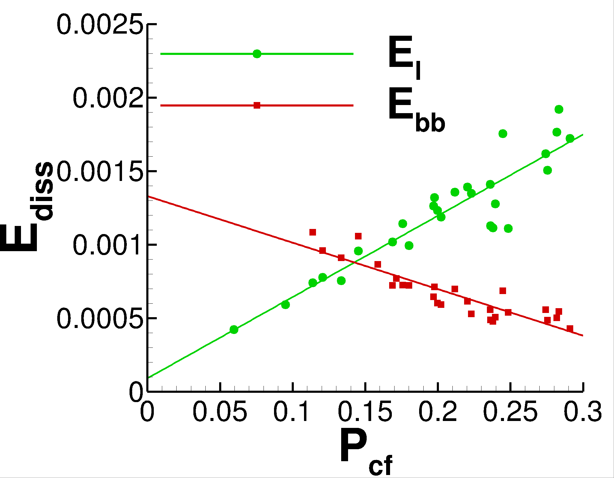
Figure 5: Energy dissipation from breaking and reformation of the bridges and other non–linear effects as a function of $P_{\rm cf}$ averaged over $15$ cycles for each $P_{\rm cf}$.

During shear, the particles move not only in the manner imposed by the moving walls, but also relative to each other. The relative motion of the particles, also referred to as the non–affine motion, is expected to play a role with regards to the breaking and reformation of the capillary bridges and subsequently the energy dissipation tied to the capillary effects, $E_{\rm bb}$. Therefore, with the particular goal of explaining the decrease of $E_{\rm bb}$ with increasing $P_{\rm cf}$ (see Figure 5) we investigate the non–affine motion of the particles as a function of $P_{\rm cf}$, using the approach described in Kondic et al. (2012), and outlined briefly here.

First, for every particle $p$, we find the affine deformation matrix $A_{\rm p}(t)$ at the time $t$ with the property

$$A_{\rm p}(t)\boldsymbol{\rm{r}}_{\rm p}(t)=\boldsymbol{\rm r}_{\rm p}(t+\delta t)\,,$$ (14)

where $\boldsymbol{\rm r}_{\rm p}(t)$ is the position of the particle $p$. The non–affine motion is defined as the minimum of the mean squared displacement

$$D^{2}_{\rm min}={\rm min}\Biggl{\{}\sum_{n=1}^{m}||\boldsymbol{\rm r}_{\rm n}-\boldsymbol{\rm r}_{\rm p}-[A_{\rm n}\boldsymbol{\rm r}_{\rm n}-A_{\rm p}\boldsymbol{\rm r}_{\rm p}]||^{2}\Biggr{\}}\,,$$ (15)

where $m$ is the number of particles within the distance of $2.5d_{\rm ave}$ from the particle $p$, and $\boldsymbol{\rm r}_{\rm n}(t)$ is the position of the $n$–th particle within this distance.

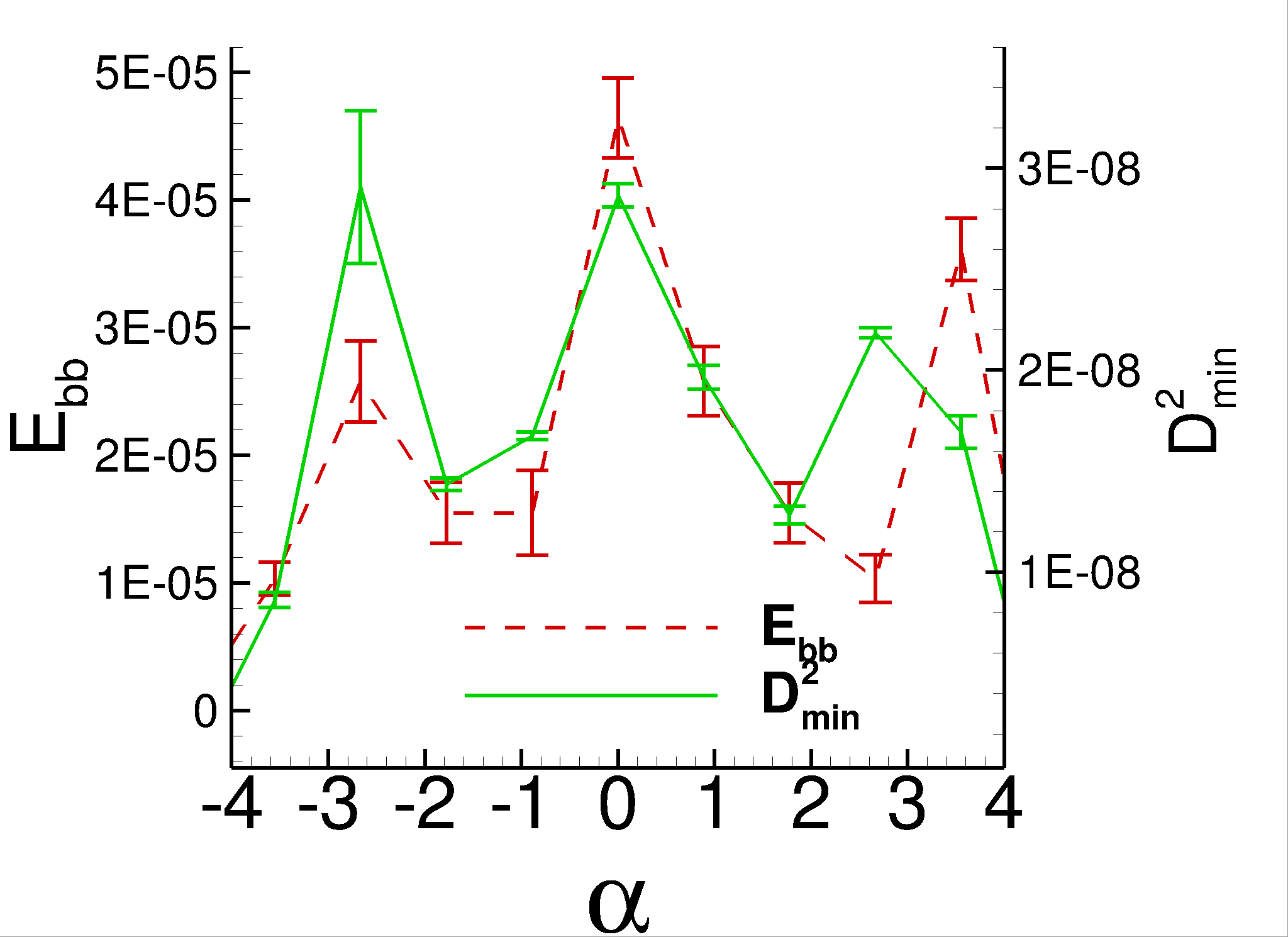
(a) $P_{\rm cf}=0.11$

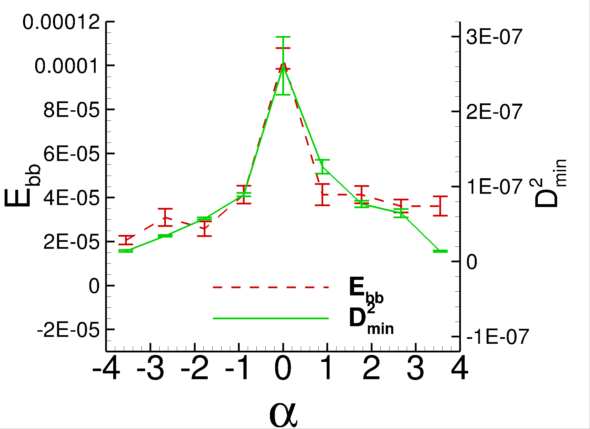
(b) $P_{\rm cf}=0.28$

Figure 6: $E_{\rm bb}$ and $D^{2}_{\rm min}$ as a function of the shearing angle, $\alpha$, for two different pressures. The results are averaged over $15$ cycles.

Figure 6 shows the energy loss from the broken bridges, $E_{\rm bb}$, as well as the measure of non-affine motion, $D^{2}_{\rm min}$, averaged over $15$ cycles, as a function of the shearing angle, $\alpha$. We average the results over $9$ equal size segments between $-\alpha_{\rm m}$ and $\alpha_{\rm m}$; we choose this number of segments so to able to show trends while still having reasonable statistics. The results are shown for one small and for one large confining pressure, $P_{\rm init}=0.08$ and $P_{\rm init}=0.4$, respectively. We see a clear correlation between $E_{\rm bb}$ and $D^{2}_{\rm min}$; similar correlation is seen for other values of $P_{\rm init}$. For $P_{\rm init}=0.08$, the magnitude of $D^{2}_{\rm min}$ is much higher than for $P_{\rm init}=0.4$; the particles have more freedom to move in non-affine manner for small confining pressures. Furthermore, the value of $D^{2}_{\rm min}$ is largest for $\alpha\approx 0$, when the shearing speed assumes its maximum.

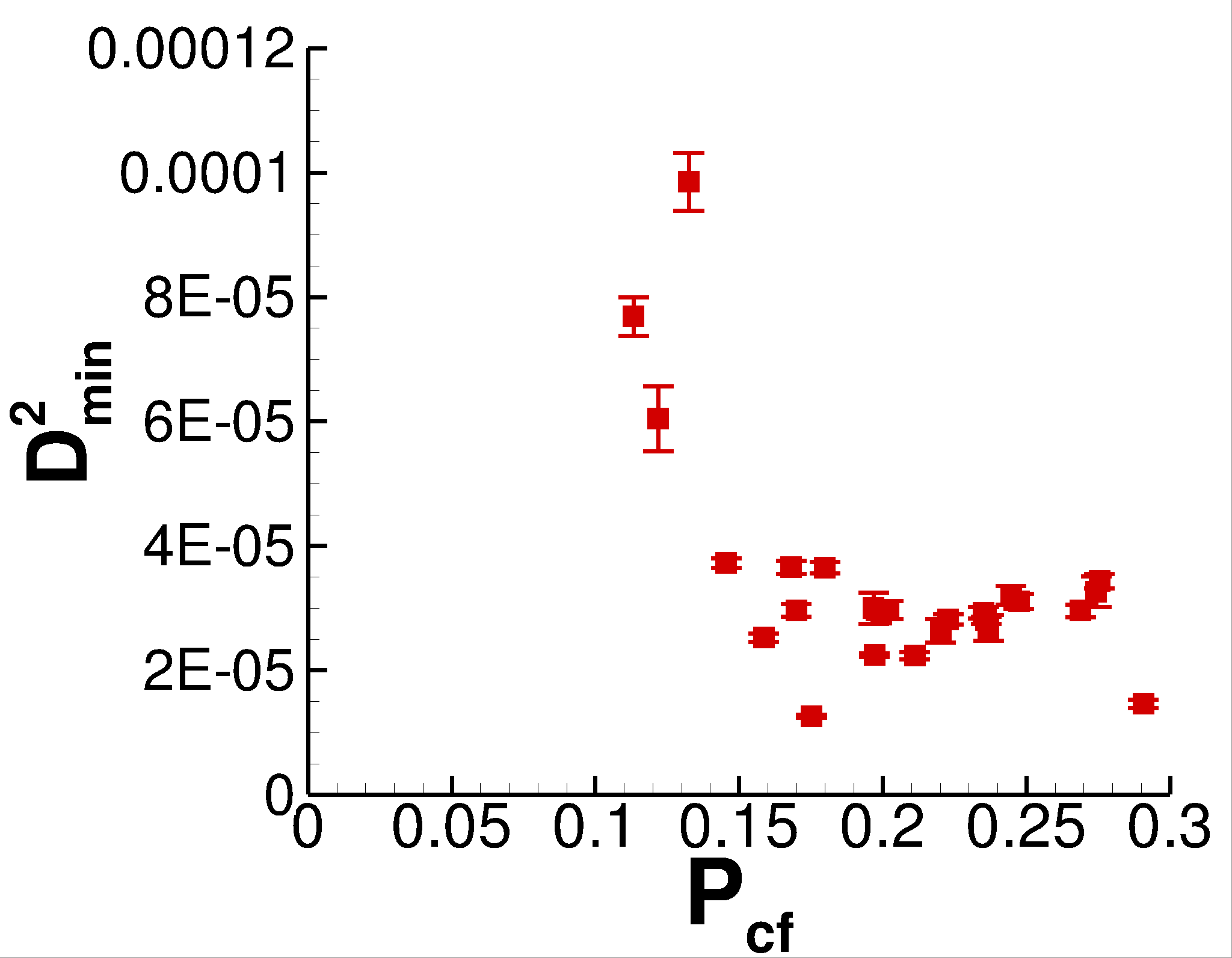
Figure 7: Non–affine motion in the wet systems averaged over $15$ cycles for each $P_{\rm cf}$.

Figure 7 summarizes the results related non-affine motion. Here we plot non–affine motion as a function of $P_{\rm cf}$, averaged over time and over $15$ cycles. An overall decreasing trend of the total non-affine motion is obvious. As a side note, we comment that we have verified that a modest increase in particle stiffness does not influence the trend of the non–affine motion with changing pressure.

The above findings show that the degree of non-affine motion is directly connected to the breaking and reforming of the bridges and reversely to the confining pressure, $P_{\rm cf}$. Therefore, a decrease of the non-affine motion explains the decrease of $E_{\rm bb}$ with increasing $P_{\rm cf}$.

We note that we have also computed non–affine motion for the frictionless and elastic particles. The results (figure not included for brevity) show significantly larger degree of non-affinity for both considered systems, compared to the frictional, inelastic one considered so far. This is expected due to reduced energy loss in elastic and/or frictionless systems.

III.0.4 Internal Cohesion

Another manner in which cohesion can influence energy dissipation is internal cohesion: capillary bridges pull particles together, leading to an enhanced friction at the contacts Fournier et al. (2005); Mason et al. (1999) as well as damping due to inelasticity (see Appendix A) that may influence the energy dissipation through changing $E_{\rm l}$ in Eq. (13). To compute this effect, we proceed as follows: In equilibrium, the capillary force between the particles leads to a compressive force and an overall elastic energy $E_{\rm el}\approx 10^{-6}$. Then, we carry out simulations with dry systems and find that this value of elastic energy corresponds to $P_{\rm cf}\approx 0.07$. This value of $P_{\rm cf}$ leads to $E_{\rm l}\approx 5\times 10^{-4}$, see Figure 5, being less than a third of the energy dissipated by breaking and reformation of capillary bridges, $E_{\rm bb}$. Therefore, the results of our simulations suggest that the breakup of capillary bridges, and not the friction or the inelasticity of collisions, is the main source of energy dissipation in weakly compressed systems and causes non-zero values of $E_{\rm diss}$ as $P_{\rm cf}\rightarrow 0$.

We note that linear extrapolation of the data shown in Figure 5 to $P_{\rm cf}<0.06$ suggests even smaller values of $E_{\rm l}$; however since simulations can not be reliably carried out for such smaller values, we conservatively choose the value of $5\times 10^{-4}$ as the upper bound for $E_{\rm l}$ for $P_{\rm cf}\approx 0$. The main point, that only a small part of energy is lost due to friction and inelasticity for small confining pressures, is clear from the overall trend of the data.

IV Conclusion

In this paper, we discussed the origin of energy dissipation in sheared wet and dry granular systems in numerical simulations following a similar setup as in recent experiments Herminghaus (2005); Fournier et al. (2005) in the regime characterized by the presence of individual capillary bridges. For small confining pressure, wet systems are stiffer than dry ones due to the cohesion by virtue of capillary bridges formed between neighboring particles, which increase the energy dissipation in two ways. For the material parameters used in the simulations, about two thirds of the dissipated energy was found to result from breaking of the capillary bridges which were elongated above their maximum length. The remaining one third is caused by the cohesion which increases the contact forces between particles and thus causes friction even in an unconfined wet granulate. An increase of applied confining pressure is found to have two consequences. First, the simulations show that energy dissipation due to breakup of capillary bridges becomes less relevant due to a decrease of the non-affine particle motion. Second, the energy dissipation for both dry and wet granulates increases linearly with externally applied confining pressure due to increased particle–particle friction. Thus for sufficiently large confining pressure energy dissipation is always dominated by friction between grains. We expect that the exact proportions describing relevance of various energy loss mechanisms may depend on the material parameters of the granular particles, however the main conclusion is general: for sufficiently small pressures, the dominant part of the energy loss is due to the effects related to cohesion, and in particular due to breakups of capillary bridges.

Appendix A Details of Simulation Techniques

The particles in the considered numerical system are modeled as 2D soft frictional inelastic circular particles that interact via normal and tangential forces, specified here in nondimensional form, using ${\bar{d}},~{}m,~{}\tau_{\rm c}$ as the length, mass and time scale introduced in the main text of the paper.

Dimensionless normal force between $i$–th and $j$–th particle is

$$\boldsymbol{F}_{\rm i,j}^{\rm n}=k_{\rm n}x_{\rm i,j}\boldsymbol{n}-\eta_{\rm n}\overline{m}\boldsymbol{v}_{\rm i,j}^{\rm n}\,,$$ (16)

where $\boldsymbol{v}_{\rm i,j}^{\rm n}$ is the relative normal velocity, $\overline{m}$ is reduced mass, $x_{\rm i,j}=d_{\rm ave}-r_{\rm i,j}$ is the amount of compression, with $d_{\rm ave}={(d_{\rm i}+d_{\rm j})/2}$ and $d_{\rm i}$, $d_{\rm j}$ diameters of the particles $i$ and $j$. The distance of the centers of $i$–th and $j$–th particle is denoted as $r_{\rm i,j}$. Parameter $\eta_{\rm n}$ is the damping coefficient in the normal direction, related to the coefficient of restitution $e$.

We implement the Cundall–Strack model for static friction Cundall and Strack (1979). The tangential spring $\boldsymbol{\xi}$ is introduced between particles for each new contact that forms at time $T=T_{0}$ and is used to determine the tangential force during the contact of particles. Due to the relative motion of particles, the spring length $\xi$ evolves as $\xi=\int_{T_{0}}^{T}\boldsymbol{v}_{\rm i,j}^{\rm t}(t)dt$ with $\boldsymbol{v}_{\rm i,j}^{\rm t}=\boldsymbol{v}_{\rm i,j}-\boldsymbol{v}_{\rm i,j}^{\rm n}$ and $\boldsymbol{v}_{\rm i,j}$ being the relative velocity of particles $i,~{}j$. The tangential direction is defined as $\boldsymbol{t}={\boldsymbol{v}_{\rm i,j}^{\rm t}/|\boldsymbol{v}_{\rm i,j}^{\rm t}|}$. The direction of $\boldsymbol{\xi}$ evolves over time and we thus correct the tangential spring as $\boldsymbol{\xi}^{\prime}=\boldsymbol{\xi}-\boldsymbol{n}(\boldsymbol{n.\xi})$. The tangential force is set to

$$\boldsymbol{F}^{\rm t}=\min(\mu_{\rm s}|\boldsymbol{F}^{\rm n}|,|\boldsymbol{F}^{\rm t\ast}|){\boldsymbol{F}^{\rm t\ast}/|\boldsymbol{F}^{\rm t\ast}|}\,,$$ (17)

with

$$\boldsymbol{F}^{\rm t\ast}=-k_{\rm t}\boldsymbol{\xi}^{\prime}-\eta_{\rm t}m\boldsymbol{v}_{\rm i,j}^{\rm t}\,.$$ (18)

Viscous damping in the tangential direction is included in the model via the damping coefficient $\eta_{\rm t}=\eta_{\rm n}$.

References

- Faure et al. (2001) A. Faure, P. York, and R. Rowe, Eur. J. Pharm. Biopharm. 52, 269 (2001).
- Leuenberger (2001) H. Leuenberger, Eur. J. Pharm. Biopharm. 52, 279 (2001).
- Paul and Sharma (1999) W. Paul and C. P. Sharma, J. Mater. Sci. Mater. Med. 10, 383 (1999).
- Komlev et al. (2002) V. Komlev, S. Barinov, and E. Koplik, Biomaterials 23, 3449 (2002).
- Simons and Fairbrother (2000) S. Simons and R. Fairbrother, Powder Tech. 110, 44 (2000).
- Litster and Ennis (2004) J. Litster and B. Ennis, Engineering of Granulation Processes: Particle Technologies Series, Springer Netherlands (Springer Netherlands, 2004).
- Realpe and Velázquez (2008) A. Realpe and C. Velázquez, Chem. Eng. Sci. 63, 1602 (2008).
- Shinagawa and Hirashima (1998) K. Shinagawa and Y. Hirashima, Met. and Mat. 4, 350 (1998).
- B. Bhandari and Schuck (2013) M. Z. B. Bhandari, N. Bansal and P. Schuck, Handbook of Food Powders (Woodhead Publishing, 2013).
- Géminard et al. (1999) J.-C. Géminard, W. Losert, and J. Gollub, Phys. Rev. E 59, 5881 (1999).
- Fournier et al. (2005) Z. Fournier, D. Geromichalos, S. Herminghaus, M. M. Kohonen, F. Mugele, M. Scheel, M. Schulz, B. Schulz, C. Schier, R. Seemann, et al., J. Phys. Condens. Mat. 17, 477 (2005).
- Mitarai and Nori (2006) N. Mitarai and F. Nori, Adv. in Phys. 55, 1 (2006).
- Scheel et al. (2008) M. Scheel, R. Seemann, M. D. M. M. Brinkmann, A. Sheppard, B. Breidenbach, and S. Herminghaus, Nat. Mater. 7, 189–193 (2008).
- Fiscina et al. (2012) J. Fiscina, M. Pakpour, A. Fall, N. Vandewalle, C. Wagner, and D. Bonn, Phys. Rev. E 86, 020103 (2012).
- Fall et al. (2014) A. Fall, B. Weber, M. Pakpour, N. Lenoir, N. Shahidzadeh, J. Fiscina, C. Wagner, and D. Bonn, Phys. Rev. Lett. 112, 175502 (2014).
- Brown et al. (2010) E. Brown, N. Rodenberg, J. Amend, A. Mozeika, E. Steltz, M. Zakin, H. Lipson, and H. Jaeger, Proc. Natl. Acad. Sci. 107, 18809 (2010).
- Halsey and Levine (1998) T. Halsey and A. Levine, Phys. Rev. Lett. 80, 3141 (1998).
- Herminghaus (2005) S. Herminghaus, Adv. Phys. 54, 221 (2005).
- (19) S. Karmakar, M. Schaber, A.-L. Schuhmacher, M. Scheel, M. DiMichiel, M. Brinkmann, R. Seemann, L. Kovalcinova, and L. Kondic, unpublished.
- Kovalcinova et al. (2015) L. Kovalcinova, A. Goullet, and L. Kondic, Phys. Rev. E 92, 032204 (2015).
- Kondic (1999) L. Kondic, Phys. Rev. E 60, 751 (1999).
- Willett et al. (2000) C. Willett, M. Adams, S. Johnson, and J. Seville, Langmuir 16, 9396 (2000).
- Urso et al. (1999) M. E. D. Urso, C. J. Lawrence, and M. J. Adams, J. Colloid Interface Sci. 220, 42 (1999).
- (24) Animation of the shear cycle, URL URLprovided/insertedbyeditor.
- Kondic et al. (2012) L. Kondic, X. Fang, W. Losert, C. O’Hern, and R. Behringer, Phys. Rev. E 85, 011305 (2012).
- Mason et al. (1999) T. Mason, A. Levine, D. ErtaÅ, and T. Halsey, Phys. Rev. E 60, R5044 (1999).
- Cundall and Strack (1979) P. Cundall and O. Strack, Géotechnique 29, 47 (1979).