1 Introduction

We present amplitude analyses for ${{D}^{0}}\rightarrow h^{+}h^{-}{{\pi}^{+}}{{\pi}^{-}}$ decays, where $h^{\pm}$ is either a pion or a kaon. These decay modes have the potential to make an important contribution to the determination of the $C\!P$-violating phase $\gamma~{}(\phi_{3})\equiv-\arg(V_{ud}V^{*}_{ub}/V_{cd}V^{*}_{cb})$ in ${{{B}^{-}}}\rightarrow{D}{{K}^{-}}$ and related decays [1, 2, 3, 4, 5, 6]. The all-charged final states (impossible in three-body decays of ${D}^{0}$) particularly suit the environment of hadron collider experiments, such as LHCb. The sensitivity to the weak phase can be significantly improved with a measured $D$-decay amplitude model, either to be used directly in the $\gamma$ extraction, or in order to optimize model-independent measurements [4, 7, 8, 9, 10].

A study of the rich resonance structure of these four-body decays is also of considerable interest in its own right. Figure 1.1 shows the dominant processes that contribute to the visible structure in the phase space. The color-favored tree diagram manifests as a cascade whereby a resonance decays into another resonance before decaying into the final state. Due to the identical quark content produced in the weak and spectator interactions, a given process and its $C\!P$-conjugate may arise even from the same initial state. Such processes, which we refer to as non-self-conjugate, are also known as flavor-non-specific decays as flavor-tagging is required to distinguish between the source of these two partners despite not being $C\!P$ eigenstates. The color-suppressed tree diagram and the $W$-exchange diagram result in self-conjugate intermediate states such as $\rho(770)^{0}\rho(770)^{0}$ or $\rho(770)^{0}\phi(1020)$ whose partial waves are eigenstates of $C\!P$. Certain intermediate states in ${{D}^{0}}\rightarrow K^{+}K^{-}\pi^{+}\pi^{-}$ decays, for instance $K^{*}(892)^{0}\,\bar{K}^{*}(892)^{0}$, are only accessible via the $W$-exchange diagram.

Figure 1.1: Examples of the color-favored (a), color-suppressed (b) and $W$-exchange (c) diagrams that contribute towards the resonant structure in ${{D}^{0}}\ \rightarrow\pi^{+}\pi^{-}\pi^{+}\pi^{-}$ and ${{D}^{0}}\rightarrow K^{+}K^{-}\pi^{+}\pi^{-}$ decays.

The decay ${{D}^{0}}\rightarrow\pi^{+}\pi^{-}\pi^{+}\pi^{-}$ provides an excellent environment to study the properties of the $a_{1}(1260)^{+}$ meson, whose width is an unresolved question, currently given as $250-600\mathrm{\,Me\kern-1.00006ptV}$ in the Particle Data Group’s Review of Particle Physics (PDG) [11]. The only previous analysis of the ${{D}^{0}}\rightarrow\pi^{+}\pi^{-}\pi^{+}\pi^{-}$ amplitude structure was published by the FOCUS collaboration based on approximately $6000$ ${{D}^{0}},{{\kern 1.99997pt\overline{\kern-1.99997ptD}{}}{}^{0}}\rightarrow\pi^{+}\pi^{-}\pi^{+}\pi^{-}$ signal events [12]. The analysis presented here benefits from the ability to distinguish ${D}^{0}$ from ${\kern 1.99997pt\overline{\kern-1.99997ptD}{}}{}^{0}$ decays and a larger data sample of approximately $7000$ signal events.

Based on the four-body amplitude formalism and analysis software used in the ${{D}^{0}}\rightarrow K^{+}K^{-}\pi^{+}\pi^{-}$ amplitude analysis performed by the CLEO collaboration [13], we introduce significant improvements especially in the parametrization of three-body resonances. Using a state-of-the-art parametrization of the $a_{1}(1260)^{+}$ lineshape, we present new measurements of the $a_{1}(1260)^{+}$ mass and width. By utilizing different parametrizations, we confirm a significant dependence of the measured width on the lineshape itself. We also observe contributions from the decay modes ${{D}^{0}}\ \rightarrow a_{1}(1640)^{+}\,\pi^{-}$ and ${{D}^{0}}\ \rightarrow\pi(1300)^{+}\,\pi^{-}$, not seen in previous analyses and provide model-independent complex lineshapes for the $a_{1}(1260)^{+}$, $a_{1}(1640)^{+}$ and $\pi(1300)^{+}$ mesons.

In addition to our new ${{D}^{0}}\rightarrow\pi^{+}\pi^{-}\pi^{+}\pi^{-}$ analysis, we also revisit the CLEO ${{D}^{0}}\rightarrow K^{+}K^{-}\pi^{+}\pi^{-}$ data using the improved formalism and analysis procedures presented in this paper. Prior to the CLEO analysis, an amplitude analysis of the decay ${{D}^{0}}\rightarrow K^{+}K^{-}\pi^{+}\pi^{-}$ was also performed by FOCUS [14].

This article is structured as follows: After an introduction to the CLEO II.V, CLEO III, and CLEO-c experiments in Sec. 2 and a description of the event selection in Sec. 3, the amplitude formalism and its implementation is described in Sec. 4 and Sec. 5, respectively. The results of the fit to data, including a model-dependent measurement of the fractional $C\!P$-even content and search for direct $C\!P$ violation, are presented in Sec. 6 and Sec. 7. Systematic uncertainties are outlined in Sec. 8, and our conclusions are given in Sec. 9. Additional technical details of the analyses can be found in the appendices and supplementary material.

2 Data Set and CLEO Detector

The data analyzed in this paper were produced in symmetric $e^{+}e^{-}$ collisions at CESR between 1995 and 2008, and collected with three different configurations of the CLEO detector: CLEO II.V, CLEO III, and CLEO-c.

In CLEO II.V [15, 16] tracking was provided by a three-layer double-sided silicon vertex detector, and two drift chambers. Charged particle identification came from $dE/dx$ information in the drift chambers, and time-of-flight (TOF) counters inserted before the calorimeter. For CLEO III [17] a new silicon vertex detector was installed, and a ring imaging Cherenkov (RICH) detector was deployed to enhance the particle identification abilities [18]. In CLEO-c, the vertex detector was replaced with a low-mass wire drift chamber [19]. A superconducting solenoid supplied a 1.5 T magnetic field for CLEO II.V and III, and 1 T for CLEO-c operation, where the average particle momentum was lower. In all detector configurations, neutral pion and photon identification was provided by a 7800-crystal CsI electromagnetic calorimeter.

Four distinct data sets are analyzed in the present study:

1. approximately 9 $\rm fb^{-1}$ accumulated at $\sqrt{s}\approx 10$ GeV by the CLEO II.V detector;

2. a total of 15.3 $\rm fb^{-1}$ accumulated by the CLEO III detector in an energy range $\sqrt{s}=7.0-11.2$ GeV, with over 90% of this sample taken at $\sqrt{s}=9.5-10.6$ GeV;

3. 818 $\rm pb^{-1}$ collected at the $\psi(3770)$ resonance by the CLEO-c detector;

4. a further 600 $\rm pb^{-1}$ taken by CLEO-c at $\sqrt{s}=4170$ MeV,

where $\sqrt{s}$ is the total energy delivered by the beam in the center-of-mass system (CMS). These samples are referred to as the CLEO II.V, CLEO III, CLEO-c 3770 and CLEO-c 4170 data sets, respectively.

Detector response is studied with GEANT-based [20] Monte Carlo (MC) simulations of each detector configuration, in which the MC events are processed with the same reconstruction algorithm as used for data.

3 Event Selection

We select events where one neutral $D$ meson decays either into a $\pi^{+}\pi^{-}\pi^{+}\pi^{-}$ or $K^{+}K^{-}\pi^{+}\pi^{-}$ final state. The analysis considers two classes of signal decays, for both of which information on the quantum numbers of the meson decaying to the signal mode is provided by an event tag.

1. Flavor-tagged decays are selected from the CLEO II.V and CLEO III data sets, in which the flavor of the decaying meson is determined by the charge of the ‘slow pion’, $\pi_{s}$, in the $D^{*+}\rightarrow{{D}^{0}}\pi^{+}_{s}$ decay chain. Flavor-tagged decays are also selected from the two CLEO-c data sets, where here the tag is obtained through the charge of a kaon associated with the decay of the other $D$ meson in the event. The wrong tag fractions for each data set are represented by the parameter $w$, given in Ref. [13].

2. $C\!P$-tagged decays are selected in the CLEO-c 3770 data set alone. In $\psi(3770)$ decays the $D-\overline{D}$ pair is produced coherently. Therefore, the $C\!P$ of the signal $D$ can be determined if the other $D$ meson is reconstructed in a decay to a $C\!P$-eigenstate. Useful information is also obtained if the tagging meson is reconstructed decaying into the modes $K^{0}_{S}\pi^{+}\pi^{-}$ or $K^{0}_{L}\pi^{+}\pi^{-}$, for which the relative contribution of $C\!P$-even and $C\!P$-odd states is known [21].

The ${{D}^{0}}\ \rightarrow\pi^{+}\pi^{-}\pi^{+}\pi^{-}$ analysis uses only the flavor-tagged subset of the CLEO-c 3770 data sample, while ${{D}^{0}}\ \rightarrow K^{+}K^{-}\pi^{+}\pi^{-}$ makes use of all the data sets described. The selection criteria for producing the data sets of each of these classes is discussed in detail in Ref. [13] and is identical to that used in our analysis, except for a few improvements that will be highlighted where applicable.

3.1 ${{D}^{0}}\ \rightarrow\pi^{+}\pi^{-}\pi^{+}\pi^{-}$ Selection

Apart from other backgrounds, there is a source of peaking background arising from ${{D}^{0}}\rightarrow K_{S}^{0}(\rightarrow{{\pi}^{+}}{{\pi}^{-}})\,{{\pi}^{+}}\,{{\pi}^{-}}$ decays. Although this has the same final state as signal, it is an incoherent process since the $K_{S}^{0}$ lifetime is much longer than those of any other possible intermediate resonance. Therefore, $K_{S}^{0}$ decays are rejected if the invariant mass of any ${{\pi}^{+}}\,{{\pi}^{-}}$ combination is within $7.5\,\mathrm{\,Me\kern-1.00006ptV}/c^{2}$ of the world-average $K_{S}^{0}$ mass [11].

Two nearly uncorrelated kinematic variables are used to define a signal and two sideband background regions. These variables are defined as the beam-constrained mass,

$$m_{bc}\equiv\sqrt{{\left(\frac{\sqrt{s}}{2}\right)}^{2}-{\vec{p}_{D}}{}^{2}},$$ (3.1)

where $\vec{p}_{D}$ is the reconstructed three-momentum of the candidate $D$ in the CMS; and the missing energy $\Delta E$,

$$\Delta E\equiv E_{D}-\frac{\sqrt{s}}{2},$$ (3.2)

where $E_{D}$ is the total reconstructed energy of candidate $D$ in the CMS. Signal events should have missing energy close to zero and beam-constrained mass close to that of the nominal ${{D}^{0}}$ mass, $m_{D}$ [11]. By construction, the $m_{bc}$ width is a measure of the beam-energy spread while the $\Delta E$ width is dominated by the detector resolution. Candidates that satisfy $m_{bc}>1.83$ $\mathrm{\,Ge\kern-1.00006ptV}/c^{2}$ and $|\Delta E|<0.1\;\mathrm{\,Ge\kern-1.00006ptV}$ are retained for further analysis.

Figure 3.1: Distribution of ${{D}^{0}}\ \rightarrow\pi^{+}\pi^{-}\pi^{+}\pi^{-}$ candidate events in missing energy $\Delta E$ and beam constrained mass within the selection regions, which are bounded by the annulus of constant invariant mass and lines normal to it. The central region (blue) is defined as the signal region, with sideband regions (red) providing background samples.

As the sideband events are used to study the background contribution within the signal region, it is crucial to select signal and background regions with a mutual and constant invariant mass, i.e. that of the $D$ meson. First, a region of constant invariant mass is obtained by selecting events with

$$\left|\sqrt{{{\Delta E}}^{2}+{\Delta E}{\sqrt{s}}\,+{m_{bc}^{2}}}-{m_{D}}\right|<15\mathrm{\,Me\kern-1.00006ptV}/c^{2}.$$ (3.3)

This relation describes an annulus in $m_{bc}$ and $\Delta E$ space. Lines normal to this annulus of constant invariant mass have an angle of inclination

$$\theta=\arctan\left(\frac{{\sqrt{s}}+2\,\Delta E}{2\,m_{bc}}\right)$$ (3.4)

about the center of the annulus. A signal region around the $D$ mass peak is then defined by requiring $|\theta-\theta_{D}|<0.004$, where $m_{bc}=m_{D}$ and $\Delta E=0$ $\mathrm{\,Ge\kern-1.00006ptV}$ at $\theta_{D}$, as shown in Fig. 3.1. Similarly, sideband regions are defined with $|\theta-\theta_{D}|>0.006$. These criteria preserve the range of invariant mass selected throughout the kinematic variables $m_{bc}$ and $\Delta E$, ensuring the distribution of events in phase space are consistent between regions. The signal region contains $9247$ $D\rightarrow\pi^{+}\pi^{-}\pi^{+}\pi^{-}$ candidates.

To estimate the signal purity of the sample, a two-dimensional unbinned maximum likelihood fit to $m_{bc}$ and $\Delta E$ is performed in the whole range. While the signal peak is modeled with a sum of three (two) Gaussian functions, the combinatorial background is described by an ARGUS [22] (linear) function in $m_{bc}$ ($\Delta E$). The number of signal events within the signal region is estimated from the fit result displayed in Fig. 3.2, to be $7250\pm 56\textrm{ (stat)}\pm 46\textrm{ (syst)}$ events, where the first uncertainty is statistical and second is systematic. The signal fraction $f_{\rm Sig}$, in this region is $f_{\rm Sig}=(78.4\pm 0.6\textrm{ (stat)}\pm 0.5\textrm{ (syst)})\%$. These systematic uncertainties are estimated by repeating the fit with different appropriate probability density function (PDF) hypotheses. As we observed a negligible impact of the background on our analysis, further improvements of the signal purity were not studied.

Figure 3.2: Beam constrained mass (a) and missing energy (b) distribution of ${{D}^{0}}\ \rightarrow\pi^{+}\pi^{-}\pi^{+}\pi^{-}$ candidates, overlaid with the projections of the fitted PDF (solid black line). The signal component is shown in blue (dashed) and the background component in red (dashed).

3.2 ${{D}^{0}}\ \rightarrow K^{+}K^{-}\pi^{+}\pi^{-}$ Selection

With respect to Ref. [13], we veto the ${\pi}^{+}$ ${\pi}^{-}$ invariant mass region around the $K_{S}^{0}$ mass, which removes essentially all peaking background from ${{D}^{0}}\rightarrow K_{S}^{0}(\rightarrow{{\pi}^{+}}{{\pi}^{-}})\,{{K}^{+}}\,{{K}^{-}}$, greatly simplifying our analysis. The $K_{S}^{0}$ veto depends on the CLEO configuration, as the mass resolution is better for data collected with the CLEO-c configurations. For data collected with CLEO (CLEO-c), the ${{\pi}^{+}}\,{{\pi}^{-}}$ invariant mass combination does not fall within $16.5\,(12)\mathrm{\,Me\kern-1.00006ptV}/c^{2}$ of the world-average $K_{S}^{0}$ mass.

In addition, for the flavor-tagged data, several changes have been applied with respect to Ref. [13]. The CLEO II.V minimum track momenta cut for the $D$ daughters is raised to $275\mathrm{\,Me\kern-1.00006ptV}/c$ as the MC was found not to represent the data sufficiently well below this value. As in Ref. [13], the kinematic variables that describe signal in the CLEO II.V and CLEO III samples are the reconstructed $D$ mass $m_{KK\pi\pi}$, and the mass difference between the $D^{*}$ and $D$ candidates, $\Delta m$. We take advantage of the possibility to ensure a constant $D$-candidate invariant mass range across different kinematic regions. For CLEO II.V, we choose $|m_{KK\pi\pi}-m_{D}|<5\;\mathrm{\,Me\kern-1.00006ptV}/c^{2}$; for CLEO III, we require that $m_{KK\pi\pi}$ is between ($m_{D}-11.2$) and ($m_{D}+8.3)\,\mathrm{\,Me\kern-1.00006ptV}/c^{2}$. For CLEO-c 3770, we utilize the criteria given in Eq. (3.3); for CLEO-c 4170 Eq. (3.3) is also used, but the tolerance of the annulus of constant invariant mass, with respect to $m_{D}$, is reduced from $15$ to $10\,\mathrm{\,Me\kern-1.00006ptV}/c^{2}$ in order to boost the signal purity in this sample. The signal and sidebands definitions in the respective accompanying kinematic variables ($\Delta m$ or $m_{bc}$) are defined accordingly in Table 3.1. In the CLEO II.V and CLEO III (CLEO-c 3770) samples, signal candidates are chosen to have $\Delta m$ ($m_{bc}$) near the expected value for signal $D$ decays. In the CLEO-c 4170 sample, we isolate our signal $D$ candidates from ${D}^{*}{{\kern 1.99997pt\overline{\kern-1.99997ptD}{}}}{}^{*}$ events, which have the highest rate and intrinsic purity [23].

The procedure to measure the purity in the signal region of each sample is identical to that of the previous analysis [13]. The events retained for the amplitude analysis and signal fractions for the improved selection criteria are given in Table 3.2.

Table 3.1: Signal region and sideband definitions in the $\Delta m$ or $m_{bc}$ kinematic variable, for flavor-tagged ${{D}^{0}}\ \rightarrow K^{+}K^{-}\pi^{+}\pi^{-}$ data in the different CLEO configurations.

Sample	Signal region	Sideband
CLEO II.V	$144.6\;\mathrm{\,Me\kern-0.80005ptV}/c^{2}<\Delta m<146.2\;\mathrm{\,Me\kern-0.80005ptV}/c^{2}$	$148.5\;\mathrm{\,Me\kern-0.80005ptV}/c^{2}<\Delta m<160.0\;\mathrm{\,Me\kern-0.80005ptV}/c^{2}$
CLEO III	$144.6\;\mathrm{\,Me\kern-0.80005ptV}/c^{2}<\Delta m<146.1\;\mathrm{\,Me\kern-0.80005ptV}/c^{2}$	$148.5\;\mathrm{\,Me\kern-0.80005ptV}/c^{2}<\Delta m<160.0\;\mathrm{\,Me\kern-0.80005ptV}/c^{2}$
CLEO-c 3770	$|m_{bc}-m_{D}|<0.005\;\mathrm{\,Ge\kern-0.80005ptV}/c^{2}$	$1.834\;\mathrm{\,Ge\kern-0.80005ptV}/c^{2}<m_{bc}<1.854\;\mathrm{\,Ge\kern-0.80005ptV}/c^{2}$
		$1.876\;\mathrm{\,Ge\kern-0.80005ptV}/c^{2}<m_{bc}<1.890\;\mathrm{\,Ge\kern-0.80005ptV}/c^{2}$
CLEO-c 4170	$2.005\;\mathrm{\,Ge\kern-0.80005ptV}/c^{2}<m_{bc}<2.030\;\mathrm{\,Ge\kern-0.80005ptV}/c^{2}$	$1.880\;\mathrm{\,Ge\kern-0.80005ptV}/c^{2}<m_{bc}<1.920\;\mathrm{\,Ge\kern-0.80005ptV}/c^{2}$

Table 3.2: Updated number of signal candidates and fractions in the signal region, for flavor-tagged ${{D}^{0}}\ \rightarrow K^{+}K^{-}\pi^{+}\pi^{-}$ data in the different CLEO configurations.

Sample	Signal candidates	$f_{\rm Sig}$
CLEO II.V	237	$0.759\pm 0.019$
CLEO III	1163	$0.898\pm 0.004$
CLEO-c 3770	1300	$0.871\pm 0.005$
CLEO-c 4170	598	$0.694\pm 0.010$

4 Amplitude Analysis Formalism

Previous four-body amplitude analyses of $D$ decays have been performed by the Mark III collaboration for ${D}\rightarrow\overline{K}\pi\pi\pi$ comprising a total of four Cabibbo-favored decay modes modes of ${D}^{0}$ and ${D}^{+}$ [24], FOCUS for ${{D}^{0}}\rightarrow\pi^{+}\pi^{-}\pi^{+}\pi^{-}$, $K^{+}K^{-}\pi^{+}\pi^{-}$, $K^{-}K^{-}K^{+}\pi^{+}$ [12, 14, 25] and most recently, for the decay ${{D}^{0}}\rightarrow K^{+}K^{-}\pi^{+}\pi^{-}$, by CLEO [13]. Here, we further develop the formalism and analysis software used in Ref. [13]. Key differences are in the formalism used for the spin factors, where we now use a more consistent and intuitive implementation of the Zemach formalism [26, 27, 28], and an improved description of the lineshapes of resonances decaying to three-body final states.

The differential decay rate of a ${{D}^{0}}$ meson with mass, $m_{{{D}^{0}}}$, decaying into four pseudoscalar particles with four-momenta $p_{i}=(E_{i},\,\vec{p}_{i})\,(i=1,2,3,4)$ is given by

$$\text{d}\Gamma=\frac{1}{2\,m_{{{D}^{0}}}}\,|A_{{{D}^{0}}}(\mathbf{x})|^{2}\,\mathrm{d}\Phi_{4}\,,$$ (4.1)

where the transition amplitude $A_{{{D}^{0}}}(\mathbf{x})$, describes the dynamics of the interaction, $\mathrm{d}\Phi_{4}$ is the four-body phase space element [29], and $\mathbf{x}$ represents a unique set of kinematic conditions within the phase space of the decay. Each final state particle contributes three observables, manifesting in their three-momentum, summing up to twelve observables in total. Four of them are redundant due to four-momentum conservation and the overall orientation of the system can be integrated out. The remaining five independent degrees of freedom unambiguously determine the kinematics of the decay. Convenient choices for the kinematic observables include the invariant mass combinations of the final state particles

$$m^{2}_{ij} =(p_{i}+p_{j})^{2},$$

$$m^{2}_{ijk} =(p_{i}+p_{j}+p_{k})^{2}\,$$ (4.2)

or acoplanarity and helicity angles [30, 31]. It is however important to take into account that, while $m^{2}_{12},m^{2}_{23}$ are sufficient to fully describe a three-body decay, the obvious extension to four-body decays with $m^{2}_{ij},m^{2}_{ijk}$ requires additional care, as these variables alone are insufficient to describe the parity-odd moments possible in four-body kinematics.

In practice, we do not need to choose a particular five-dimensional basis, but use the full four-vectors of the decay in our analysis. The dimensionality is handled by the phase space element which can be written in terms of any set of five independent kinematic observables, $\mathbf{x}=(x_{1},\ldots,x_{5})$, as

$$\mathrm{d}\Phi_{4}=\phi_{4}(\mathbf{x})\,\mathrm{d}^{5}x,$$ (4.3)

where $\phi_{4}(\mathbf{x})=\left|\frac{\partial\Phi_{4}}{\partial(x_{1},\ldots x_{5})}\right|$ is the phase space density. In contrast to three-body decays, the four-body phase space density function is not flat in the usual kinematic variables. Therefore, an analytic expression for $\phi_{4}$ is taken from Ref. [32].

The total amplitude for the ${{D}^{0}}\rightarrow h_{1}\,h_{2}\,h_{3}\,h_{4}$ decay is given by the coherent sum over all intermediate state amplitudes $A_{i}(\mathbf{x})$, each weighted by a complex coefficient $a_{i}=|a_{i}|\,e^{i\,\phi_{i}}$ to be measured from data,

$$A_{{{D}^{0}}}(\mathbf{x})=\sum_{i}a_{i}\,A_{i}(\mathbf{x})\,.$$ (4.4)

To construct $A_{i}(\mathbf{x})$, the isobar approach is used, which assumes that the decay process can be factorized into subsequent two-body decay amplitudes [33, 34, 35]. This gives rise to two different decay topologies; quasi two-body decays ${{D}^{0}}\rightarrow(R_{1}\rightarrow h_{1}\,h_{2})\,(R_{2}\rightarrow h_{3}\,h_{4})$ or cascade decays ${{D}^{0}}\rightarrow h_{1}\,\left[R_{1}\rightarrow h_{2}\,(R_{2}\rightarrow h_{3}\,h_{4})\right]$. In either case, the intermediate state amplitude is parameterized as a product of form factors $B_{L}$, included for each vertex of the decay tree, Breit-Wigner propagators $T_{R}$, included for each resonance $R$, and an overall angular distribution represented by a spin factor $S$,

$$A_{i}(\mathbf{x})=B_{L_{D}}(\mathbb{x})\,[B_{L_{R_{1}}}(\mathbf{x})\,T_{R_{1}}(\mathbf{x})]\,[B_{L_{R_{2}}}(\mathbf{x})\,T_{R_{2}}(\mathbf{x})]\,S_{i}(\mathbf{x})\,.$$ (4.5)

As the ${{\pi}^{+}}{{\pi}^{-}}{{\pi}^{-}}{{\pi}^{+}}$ final state involves two pairs of indistinguishable pions, the amplitudes are Bose-symmetrized and therefore symmetric under exchange of like-sign pions.

We define the $C\!P$-conjugate phase space point $\overline{\mathbf{x}}$ such that it is mapped onto $\mathbf{x}$ by the interchange of final state charges, and the reversal of three-momenta. If $\mathbf{x}$, $\overline{\mathbf{x}}$ are expressed as a function of the four-momenta $(E_{i},\vec{p}_{i})$ (where $i$ labels the particle), this implies for ${{D}^{0}}\rightarrow K^{+}K^{-}\pi^{+}\pi^{-}$ that

$$\overline{\mathbf{x}}\left[(E_{K^{+}},\vec{p}_{K^{+}}),(E_{K^{-}},\vec{p}_{K^{-}}),(E_{\pi^{+}},\vec{p}_{\pi^{+}}),(E_{\pi^{-}},\vec{p}_{\pi^{-}})\right]$$

$$\equiv\mathbf{x}\left[(E_{K^{-}},-\vec{p}_{K^{-}}),(E_{K^{+}},-\vec{p}_{K^{+}}),(E_{\pi^{-}},-\vec{p}_{\pi^{-}}),(E_{\pi^{+}},-\vec{p}_{\pi^{+}})\right],$$ (4.6)

and equivalently for ${{D}^{0}}\rightarrow\pi^{+}\pi^{-}\pi^{+}\pi^{-}$. The $C\!P$-conjugate of a given intermediate state amplitude, $A_{i}(x)$, is defined as

$$\overline{A}_{i}(\mathbf{x})\equiv A_{i}(\overline{\mathbf{x}}),$$ (4.7)

and the total ${\kern 1.99997pt\overline{\kern-1.99997ptD}{}}{}^{0}$ decay amplitude is defined as

$$A_{{{\kern 1.39998pt\overline{\kern-1.39998ptD}{}}{}^{0}}}(\mathbf{x}) \equiv\sum_{i}\bar{a}_{i}\,\overline{A}_{i}(\mathbf{x})=\sum_{i}\bar{a}_{i}A_{i}(\overline{\mathbf{x}}).$$ (4.8)

Unless stated otherwise, we assume $C\!P$ conservation in the ${D}^{0}$ decay, implying $\bar{a}_{i}=a_{i}$. Moreover, $C\!P$ conservation in the strong interaction is implemented in the cascade topology by the sharing of couplings between related quasi-two-body final states. For example, given the two $a_{i}$ parameters required for ${{D}^{0}}\ \rightarrow\pi^{-}a_{1}(1260)^{+}$ with $a_{1}(1260)^{+}\rightarrow\rho(770)^{0}\,\pi^{+}$ and $a_{1}(1260)^{+}\rightarrow\sigma\,\pi^{+}$, the amplitude ${{D}^{0}}\ \rightarrow\pi^{+}\,a_{1}(1260)^{-}$ with $a_{1}(1260)^{-}\rightarrow\rho(770)^{0}\,\pi^{-}$ and $a_{1}(1260)^{-}\rightarrow\sigma\,\pi^{-}$ only requires one additional global complex parameter to represent the different weak processes of $D^{0}\rightarrow a_{1}(1260)^{+}\,\pi^{-}$ and $D^{0}\rightarrow a_{1}(1260)^{-}\,\pi^{+}$, while the relative magnitude and phase of $a_{1}(1260)^{-}\rightarrow\rho(770)^{0}\,\pi^{-}$ and $a_{1}(1260)^{-}\rightarrow\sigma\,\pi^{-}$ are the same as for $a_{1}(1260)^{+}\rightarrow\rho(770)^{0}\,\pi^{+}$ and $a_{1}(1260)^{+}\rightarrow\sigma\,\pi^{+}$. For historical reasons, this constraint is only applied to the $\pi^{+}\pi^{-}\pi^{+}\pi^{-}$ final state, but, as discussed in Sec. 7, the results we obtain for the $K^{+}K^{-}\pi^{+}\pi^{-}$ final state are also compatible with $C\!P$  conservation in the strong interaction.

4.1 Form Factors and Resonance Lineshapes

To account for the finite size of the decaying resonances, the Blatt-Weisskopf penetration factors, derived in Ref. [36] by assuming a square well interaction potential with radius $r_{\rm BW}$, are used as form factors, $B_{L}$. They depend on the breakup momentum $q$, and the orbital angular momentum $L$, between the resonance daughters. Their explicit expressions are

$$B_{0}(q) =1,$$

$$B_{1}(q) =1/\sqrt{{1+(q\,r_{\rm BW})^{2}}},$$

$$B_{2}(q) =1/\sqrt{9+3\,(q\,r_{\rm BW})^{2}+(q\,r_{\rm BW})^{4}}.$$ (4.9)

Resonance lineshapes are described as function of the energy-squared, $s$, by Breit-Wigner propagators

$$T(s)=\frac{1}{M^{2}(s)-s-i\,m_{0}\,\Gamma(s)}\,,$$ (4.10)

featuring the energy-dependent mass $M(s)$ (defined below), and total width, $\Gamma(s)$. The latter is normalized to give the nominal width, $\Gamma_{0}$, when evaluated at the nominal mass $m_{0}$, i.e. $\Gamma_{0}=\Gamma(s=m_{0}^{2})$.

For a decay into two stable particles $R\rightarrow AB$, the energy dependence of the decay width can be described by

$$\Gamma_{R\rightarrow AB}^{(2)}(s)=\Gamma_{0}\,\frac{m_{0}}{\sqrt{s}}\,\left(\frac{q}{q_{0}}\right)^{2L+1}\,\frac{B_{L}(q)^{2}}{B_{L}(q_{0})^{2}}\,,$$ (4.11)

where $q_{0}$ is the value of the breakup momentum at the resonance pole [37].

The energy-dependent width for a three-body decay $R\rightarrow ABC$, on the other hand, is considerably more complicated and has no analytic expression in general. However, it can be obtained numerically by integrating the transition amplitude-squared over the phase space,

$$\Gamma_{R\rightarrow ABC}^{(3)}(s)=\frac{1}{2\,\sqrt{s}}\,\int|A_{R\rightarrow ABC}|^{2}\,\text{d}\Phi_{3},$$ (4.12)

and therefore requires knowledge of the resonant substructure. The three-body amplitude $A_{R\rightarrow ABC}$ can be parameterized similarly to the four-body amplitude in Eq. (4.5). In particular, it includes form factors and propagators of intermediate two-body resonances.

Both Eq. (4.11) and Eq. (4.12) give only the partial width for the decay into a specific channel. To obtain the total width, a sum over all possible decay channels has to be performed,

$$\Gamma(s)=\sum_{i}g_{i}\,\Gamma_{i}(s),$$ (4.13)

where the coupling strength to channel $i$, is given by $g_{i}$. Branching fractions ${\cal B}_{i}$ are related to the couplings $g_{i}$ via the equation [11]

$${\cal B}_{i}=\int_{s_{min}}^{\infty}\frac{g_{i}\,m_{0}\,\Gamma_{i}(s)}{|M^{2}(s)-s-i\,m_{0}\,\sum_{j}g_{j}\,\Gamma_{j}(s)|^{2}}\,\text{d}s.$$ (4.14)

As experimental values are usually only available for the branching fractions, Eq. (4.14) needs to be inverted to obtain values for the couplings. In practice, this is solved by minimizing the quantity $\chi^{2}(g)=\sum_{i}\left[\mathcal{B}_{i}-\mathcal{I}_{i}(g)\right]^{2}/\Delta\mathcal{B}_{i}^{2}$, where $\mathcal{I}_{i}(g)$ denotes the right-hand side of Eq. (4.14).

The energy-dependent mass follows from the decay width via the Kramers-Kronig dispersion relation [38, 39]:

$$M^{2}(s)=m_{0}^{2}+\frac{m_{0}}{\pi}\,\int_{s_{min}}^{\infty}\left(\frac{\Gamma(s^{\prime})}{s-s^{\prime}}-\frac{\Gamma(s^{\prime})}{m_{0}^{2}-s^{\prime}}\right)\,\text{d}s^{\prime}.$$ (4.15)

Here, the energy-dependent mass is renormalized such that $M^{2}(s=m_{0}^{2})=m_{0}^{2}$. In practice, the energy-dependent mass is often approximated as being constant, i.e. $M^{2}(s)=m_{0}^{2}$, since its calculation requires a detailed understanding of the decay width for arbitrarily large energies and is computationally expensive. This is usually justified as the energy-dependent mass needs to satisfy the condition,

$$\frac{\text{d}M^{2}(s)}{\text{d}s}\bigg{\rvert}_{s=m_{0}^{2}}=0,$$ (4.16)

such that $M^{2}(s)$ is indeed, approximately constant near the on-shell mass [40]. Larger dispersive effects are thus only expected for very broad resonances.

The treatment of the lineshape for various resonances considered in this analysis is described in what follows. The nominal masses and widths of the resonances are taken from the PDG [11] with the exceptions described below. We assume an energy-independent mass unless otherwise stated.

For the broad scalar resonance $\sigma$, the model from Bugg is used [41]. Besides $\sigma\rightarrow\pi\pi$ decays, it includes contributions from the decay modes $\sigma\rightarrow KK$, $\sigma\rightarrow\eta\eta$ and $\sigma\rightarrow\pi\pi\pi\pi$ as well as dispersive effects due to the channel opening of the latter. We use the Gournaris-Sakurai parametrization for the $\rho(770)^{0}\rightarrow\pi\pi$ propagator which provides an analytical description of the dispersive term, $M^{2}(s)$ [42]. The energy-dependent width of the $f_{0}(980)$ resonance is given by the sum of the partial widths into the $\pi\pi$ and $KK$ channels [43],

$$\Gamma_{f_{0}(980)}(s)=g_{\pi\pi}\,\Gamma^{(2)}_{f_{0}(980)\rightarrow\pi\pi}(s)+g_{KK}\,\Gamma^{(2)}_{f_{0}(980)\rightarrow KK}(s),$$ (4.17)

where the coupling constants $g_{\pi\pi}$ and $g_{KK}$, as well as the mass and width are taken from a measurement performed by the BES Collaboration [44]. The total decay widths for both the $f_{2}(1270)$ and the $f_{0}(1370)$ meson take the channels $\pi\pi,KK,\eta\eta$ and $\pi\pi\pi\pi$ into account. While the two-body partial widths are described by Eq. (4.11), a model for the partial width for a decay into four pions is taken from Ref. [45]. The corresponding branching fractions are taken from the PDG [11]. The nominal mass and width of the $f_{0}(1370)$ resonance are taken from an LHCb measurement [46]. Equation (4.11) is used for all other resonances decaying into a two-body final state.

To describe the decay width of the axial vector resonance $a_{1}(1260)$, the decay channels $\pi\pi\pi$ and $K\bar{K}\pi$ are considered,

$$\Gamma_{a_{1}(1260)}(s)=g_{\pi\pi\pi}\,\Gamma^{(3)}_{a_{1}(1260)\rightarrow\pi\pi\pi}(s)+g_{K\bar{K}\pi}\,\Gamma^{(3)}_{a_{1}(1260)\rightarrow K\bar{K}\pi}(s),$$ (4.18)

where isospin symmetry is assumed, i.e. $\Gamma^{(3)}_{a_{1}(1260)^{+}\rightarrow{{\pi}^{+}}{{\pi}^{-}}{{\pi}^{+}}}(s)=\Gamma^{(3)}_{a_{1}(1260)^{+}\rightarrow\pi^{0}\pi^{0}{{\pi}^{+}}}(s)$. The partial width $\Gamma^{(3)}_{a_{1}(1260)\rightarrow K\bar{K}\pi}(s)$ is calculated from Eq. (4.12) assuming the decay proceeds entirely via $a_{1}(1260)\rightarrow K^{*}(892)\,K$. The corresponding branching fraction is taken from a CLEO analysis of hadronic $\tau$ decays [47]. The calculation of the partial width $\Gamma^{(3)}_{a_{1}(1260)\rightarrow\pi\pi\pi}(s)$ is more complicated due to the fact that it requires information about the three pion Dalitz plot structure of the $a_{1}(1260)$ resonance whose determination in turn, needs the propagator as input. For this reason, we follow an iterative approach. The initial amplitude fit, described in Sec. 6, is performed using an energy-dependent width distribution derived from an uniform phase space population. Afterwards, the energy-dependent width is recalculated with the results of the substructure analysis and the amplitude fit is subsequently repeated with the new propagator. It is found that the energy-dependent width is not highly sensitive to the details of the Dalitz plot as this procedure converges after a few iterations. As the $a_{1}(1260)$ resonance is very broad, the dispersive term is calculated as well. Figure 4.1 shows the final iteration of the energy-dependent width and mass. The energy-dependent width varies strongly around $s\approx 0.8\;\mathrm{\,Ge\kern-1.00006ptV}^{2}$ where the energy of the ${{\pi}^{+}}\,{{\pi}^{-}}$ subsystem is equal to the $\rho(770)^{0}$ on-shell mass. Around $s=2\;\mathrm{\,Ge\kern-1.00006ptV}^{2}$, a small hump develops due to the opening of the $K\bar{K}\pi$ channel. The energy-dependent mass indeed shows a plateau around the nominal mass as expected. Note that as the condition of Eq. (4.16) is not explicitly enforced by Eq. (4.15), it serves as an independent check of whether the main thresholds have been included  [38, 47].

For the resonances $\pi(1300)$, $a_{1}(1640)$ and $\pi_{2}(1670)$, the energy-dependent width is obtained via the same iterative procedure as for the $a_{1}(1260)$ resonance. In case of the $\pi_{2}(1670)$ meson, the $K\bar{K}\pi$ and $\omega\rho(770)^{0}$ thresholds are included with the PDG branching fractions taken from Ref. [11], otherwise only decays to three pions are considered. In the ${{D}^{0}}\rightarrow K^{+}K^{-}\pi^{+}\pi^{-}$ analysis, resonant decays of the $K_{1}(1270)$ and $K_{1}(1400)$ mesons into the $K\rho(770)^{0}$, $K^{*}(892)\pi$, $K_{0}^{*}(1430)\pi$, $Kf_{0}(1370)$ and $K\omega$ decay channels are taken into account assuming the lowest possible angular momentum state. For the purpose of evaluating the energy-dependent widths of the excited kaons, these decay channels are assumed to be incoherent and the branching fractions from the PDG are used [11]. The same procedure is applied to obtain the energy-dependent width for the $K^{*}(1410)$ and $K^{*}(1680)$ resonances. In their case, the decay channels $K\rho(770)^{0}$, $K^{*}(892)\pi$ and $K\pi$ are considered. For the $K^{*}(1410)$ meson there are only upper limits for the branching fractions into the $K\rho(770)^{0}$ and $K^{*}(892)\pi$ channels available. We assume no $K^{*}(1410)\rightarrow K\rho(770)^{0}$ contribution and $\mathcal{B}[K^{*}(1410)\rightarrow K^{*}(892)\pi]=1-\mathcal{B}[K^{*}(1410)\rightarrow K\pi]=(93.4\pm 1.3)\,\%$ [11]. All energy-dependent widths not shown in this Chapter are shown in Appendix A.

Some particles may not originate from a resonance but are in a state of relative orbital angular momentum. We denote such non-resonant states by surrounding the particle system with brackets and indicate the partial wave state with an subscript; for example $(\pi\pi)_{S}$ refers to a non-resonant di-pion $S$-wave. The lineshape for non-resonant states is set to unity.

Figure 4.1: Energy-dependent width (a) and energy-dependent mass (b) for the $a_{1}(1260)$ resonance. The total width is shown in black (solid), while the partial widths $\Gamma^{(3)}_{a_{1}(1260)\rightarrow\pi\pi\pi}(s)$ and $\Gamma^{(3)}_{a_{1}(1260)\rightarrow K\bar{K}\pi}(s)$ are shown in blue (dashed) and red (dotted), respectively.

4.2 Spin Densities

The spin amplitudes are phenomenological descriptions of decay processes that are required to be Lorentz invariant, compatible with angular momentum conservation and, where appropriate, parity conservation. They are constructed in the covariant Zemach (Rarita-Schwinger) tensor formalism [26, 27, 28]. At this point, we briefly introduce the fundamental objects of the covariant tensor formalism which connect the particle’s four-momenta to the spin dynamics of the reaction and give a general recipe to calculate the spin factors for arbitrary decay trees. Further details can be found in Refs. [48, 49].

A spin-$S$ particle with four-momentum $p$, and spin projection $\lambda$, is represented by the polarization tensor $\epsilon_{(S)}(p,\lambda)$, which is symmetric, traceless and orthogonal to $p$. These so-called Rarita-Schwinger conditions reduce the a priori $4^{S}$ elements of the rank-$S$ tensor to $2S+1$ independent elements in accordance with the number of degrees of freedom of a spin-$S$ state[27, 50].

The spin projection operator $P^{\mu_{1}\dots\mu_{S}\nu_{1}\dots\nu_{S}}_{(S)}(p_{R})$, for a resonance $R$, with spin $S=\{0,1,2\}$, and four-momentum $p_{R}$, is given by [49]:

$$P_{(0)}^{\mu\nu}(p_{R}) =1$$

$$P_{(1)}^{\mu\nu}(p_{R}) =-\,g^{\mu\nu}+\frac{p_{R}^{\mu}\,p_{R}^{\nu}}{p_{R}^{2}}$$

$$P_{(2)}^{\mu\nu\alpha\beta}(p_{R}) =\frac{1}{2}\,\left[P_{(1)}^{\mu\alpha}(p_{R})\,P_{(1)}^{\nu\beta}(p_{R})+P_{(1)}^{\mu\beta}(p_{R})\,P_{(1)}^{\nu\alpha}(p_{R})\right]-\frac{1}{3}\,P_{(1)}^{\mu\nu}(p_{R})\,P_{(1)}^{\alpha\beta}(p_{R})\,,$$ (4.19)

where $g^{\mu\nu}$ is the Minkowski metric. Contracted with an arbitrary tensor, the projection operator selects the part of the tensor which satisfies the Rarita-Schwinger conditions.

For a decay process $R\rightarrow AB$, with relative orbital angular momentum $L$, between particle $A$ and $B$, the angular momentum tensor is obtained by projecting the rank-$L$ tensor $q_{R}^{\nu_{1}}\,q_{R}^{\nu_{2}}\dots\,q_{R}^{\nu_{L}}$, constructed from the relative momenta $q_{R}=p_{A}-p_{B}$, onto the spin-$L$ subspace,

$$L_{(L)\mu_{1}\dots\mu_{L}}(p_{R},q_{R})=(-1)^{L}\,P_{(L)\mu_{1}\dots\mu_{L}\nu_{1}\dots\nu_{L}}(p_{R})\,q_{R}^{\nu_{1}}\dots\,q_{R}^{\nu_{L}}.$$ (4.20)

Their $|\vec{q}_{R}|^{L}$ dependence accounts for the influence of the centrifugal barrier on the transition amplitudes. For the sake of brevity, the following notation is introduced,

$${\varepsilon}_{(S)}(R) \equiv{\varepsilon}_{(S)}(p_{R},\lambda_{R}),$$

$$P_{(S)}(R) \equiv P_{(S)}(p_{R}),$$

$$L_{(L)}(R) \equiv L_{(L)}(p_{R},q_{R}).$$ (4.21)

Following the isobar approach, a four-body decay amplitude is described as a product of two-body decay amplitudes. Each sequential two-body decay $R\rightarrow A\,B$, with relative orbital angular momentum $L_{AB}$, and total intrinsic spin $S_{AB}$, contributes a term to the overall spin factor given by

$$S_{R\rightarrow AB}(\mathbb{x}|L_{AB},S_{AB};\lambda_{R},\lambda_{A},\lambda_{B}) ={\varepsilon}_{(S_{R})}(R)\,X(S_{R},L_{AB},S_{AB})\,L_{(L_{AB})}(R)\,$$

$$\times\Phi(\mathbb{x}|S_{AB};\lambda_{A},\lambda_{B}),$$ (4.22)

where

$$\Phi(\mathbb{x}|S_{AB};\lambda_{A},\lambda_{B}) =P_{(S_{AB})}(R)\,X(S_{AB},S_{A},S_{B})\,{\varepsilon}^{*}_{(S_{A})}(A)\,{\varepsilon}^{*}_{(S_{B})}(B)\,.$$ (4.23)

Here, a polarization vector is assigned to the decaying particle and the complex conjugate vectors for each decay product. The spin and orbital angular momentum couplings are described by the tensors $P_{(S_{AB})}(R)$ and $L_{(L_{AB})}(R)$, respectively. Firstly, the two spins $S_{A}$ and $S_{B}$, are coupled to a total spin-$S_{AB}$ state, $\Phi(\mathbb{x}|S_{AB})$, by projecting the corresponding polarization vectors onto the spin-$S_{AB}$ subspace transverse to the momentum of the decaying particle. Afterwards, the spin and orbital angular momentum tensors are properly contracted with the polarization vector of the decaying particle to give a Lorentz scalar. This requires in some cases to include the tensor ${\varepsilon}_{\alpha\beta\gamma\delta}\,p_{R}^{\delta}$ via

$$X(j_{a},j_{b},j_{c})=\begin{cases}1&\mbox{if }j_{a}+j_{b}+j_{c}\;{\rm even}\\ {\varepsilon}_{\alpha\beta\gamma\delta}\,p_{R}^{\delta}&\mbox{if }j_{a}+j_{b}+j_{c}\;{\rm odd}\end{cases}\,,$$ (4.24)

where ${\varepsilon}_{\alpha\beta\gamma\delta}$ is the Levi-Civita symbol and $j$ refers to the arguments of $X$ defined in Eqs. 4.22 and 4.23. Its antisymmetric nature ensures the correct parity transformation behavior of the amplitude. The spin factor for a whole decay chain, for example $R\rightarrow(R_{1}\rightarrow AB)\,(R_{2}\rightarrow CD)$, is obtained by combining the two-body terms and performing a sum over all unobservable, intermediary spin projections

$$\sum_{\lambda_{R_{1}},\lambda_{R_{2}}}S_{R\rightarrow R_{1}R_{2}}(\mathbb{x}|L_{R_{1}R_{2}};\lambda_{R_{1}},\lambda_{R_{2}})\,S_{R_{1}\rightarrow AB}(\mathbb{x}|L_{AB};\lambda_{R_{1}})\,S_{R_{2}\rightarrow CD}(\mathbb{x}|L_{CD};\lambda_{R_{2}}),$$ (4.25)

where $\lambda_{R}=\lambda_{A}=\lambda_{B}=\lambda_{C}=\lambda_{D}=0$, $S_{AB}=S_{CD}=0$ and $S_{R_{1}R_{2}}=L_{R_{1}R_{2}}$, as only pseudoscalar initial/final states are involved.

The main difference to the formalism used in Ref. [13] is the inclusion of additional projection operators, i.e. $P_{(S_{AB})}(R)$ and the one intrinsic to $L_{(L_{AB})}(R)$, which ensure pure spin and angular momentum tensors. The spin factors for all decay topologies considered in this analysis are explicitly given in Appendix B.

4.3 Measurement Quantities

Here, we define all quantities derived from the amplitude model that are of physical importance. In order to provide implementation-independent measurements in addition to the complex coefficients $a_{i}$, we define two quantities. Firstly, the fit fractions

$$F_{i}\equiv\frac{\int\left|a_{i}\,A_{i}(\mathbf{x})\right|^{2}\,\text{d}\Phi_{4}}{\int\left|A_{{{D}^{0}}}(\mathbf{x})\right|^{2}\,\text{d}\Phi_{4}},$$ (4.26)

which are a measure of the relative strength between the different transitions. Secondly, the interference fractions are given by

$$I_{ij}\equiv\frac{\int 2\,\Re[a_{i}a^{*}_{j}\,A_{i}(\mathbf{x})A^{*}_{j}(\mathbf{x})]\,\text{d}\Phi_{4}}{\int\left|A_{{{D}^{0}}}(\mathbf{x})\right|^{2}\,\text{d}\Phi_{4}},$$ (4.27)

which measures the interference effects between amplitude pairs. Constructive interference leads to $I_{ij}>0$, while destructive interference leads to $I_{ij}<0$. Note that $\sum_{i}F_{i}+\sum_{j<k}I_{j,k}=1$.

The global fractional $C\!P$-even content is defined as,

$$F_{+}\equiv\frac{\int|A_{+}|^{2}\,\text{d}\Phi_{4}}{\int|A_{+}|^{2}+|A_{-}|^{2}\,\text{d}\Phi_{4}}$$ (4.28)

where $A_{\pm}\equiv A_{{{D}^{0}}}(\mathbf{x})\pm A_{{{\kern 1.39998pt\overline{\kern-1.39998ptD}{}}{}^{0}}}(\mathbf{x})$ is the decay amplitude for a $D$ meson in a $C\!P$-even / $C\!P$-odd state. The parameter $F_{+}$, can be determined from an amplitude model (Eq. (4.28)) or by using model-independent methods [51]; the consistency of the two techniques provides a useful cross-check of the amplitude model. The fractional $C\!P$-even content also provides useful input to the determination of the CKM phase $\gamma$ ($\phi_{3}$) in $B^{\pm}\rightarrow DK^{\pm}$ and related decays. Additionally, knowledge of $F_{+}$ for all $D$ decay final states can be used to determine the net $C\!P$-content of the $D$ meson system, which is related to the charm-mixing parameter $y_{D}$ [52].

Finally, measurements of direct $C\!P$ violation will also be reported. For this purpose, the amplitude coefficients are expressed in terms of a $C\!P$-conserving ($c_{i}$) and a $C\!P$-violating ($\Delta c_{i}$) parameter,

$$a_{i}\equiv c_{i}\,(1+\Delta c_{i}),\,\,\bar{a}_{i}\equiv c_{i}\,(1-\Delta c_{i}).$$ (4.29)

For $\Delta c_{i}=0$ there is no $C\!P$ violation between the corresponding ${D}^{0}$ and ${\kern 1.99997pt\overline{\kern-1.99997ptD}{}}{}^{0}$ intermediate state amplitudes. Note that the $C\!P$-violating parameters are included only for distinct weak decay processes as the strong interaction is assumed to be $C\!P$-conserving such that e.g. the amplitudes for the processes ${{D}^{0}}\rightarrow{{\pi}^{-}}\,\left[a_{1}(1260)^{+}\rightarrow{{\pi}^{+}}\,\rho(770)^{0}\right]$ and ${{D}^{0}}\rightarrow{{\pi}^{-}}\,\left[a_{1}(1260)^{+}\rightarrow{{\pi}^{+}}\,\sigma\right]$ share a common $\Delta c_{i}$, while having different $C\!P$-conserving parameters. As we do not measure the time distribution, we have no sensitivity to the overall phase difference between ${{D}^{0}}$ and ${{\kern 1.99997pt\overline{\kern-1.99997ptD}{}}{}^{0}}$ and thus, the phase difference between $A_{{D}^{0}}(\mathbf{x})$ and $A_{{\kern 1.39998pt\overline{\kern-1.39998ptD}{}}{}^{0}}(\mathbf{x})$ is fixed to null. From these separate amplitudes, the direct $C\!P$ violation in each amplitude is simply calculated from the fit coefficients as

$$\mathcal{A}_{CP}^{i}\equiv\frac{|a_{i}|^{2}-|\bar{a}_{i}|^{2}}{|a_{i}|^{2}+|\bar{a}_{i}|^{2}}.$$ (4.30)

In principle, the global direct $C\!P$ asymmetry can be calculated from

$$\mathcal{A}_{CP}\equiv\frac{\int|A_{{{D}^{0}}}(\mathbf{x})|^{2}\,\text{d}\Phi_{4}-\int|A_{{{\kern 1.39998pt\overline{\kern-1.39998ptD}{}}{}^{0}}}(\mathbf{x})|^{2}\,\text{d}\Phi_{4}}{\int|A_{{{D}^{0}}}(\mathbf{x})|^{2}\,\text{d}\Phi_{4}+\int|A_{{{\kern 1.39998pt\overline{\kern-1.39998ptD}{}}{}^{0}}}(\mathbf{x})|^{2}\,\text{d}\Phi_{4}},$$ (4.31)

however to avoid an unnecessary systematic uncertainty arising from the amplitude model, this will instead be determined from an asymmetry in the integrated decay rates,

$$\mathcal{A}_{CP}\equiv\frac{\Gamma({{D}^{0}}\rightarrow h^{+}h^{-}{{\pi}^{+}}{{\pi}^{-}})-{\Gamma}({{\kern 1.99997pt\overline{\kern-1.99997ptD}{}}{}^{0}}\rightarrow h^{+}h^{-}{{\pi}^{+}}{{\pi}^{-}})}{\Gamma({{D}^{0}}\rightarrow h^{+}h^{-}{{\pi}^{+}}{{\pi}^{-}})+{\Gamma}({{\kern 1.99997pt\overline{\kern-1.99997ptD}{}}{}^{0}}\rightarrow h^{+}h^{-}{{\pi}^{+}}{{\pi}^{-}})}=\frac{\bar{{\varepsilon}}_{\rm Tag}N_{{{D}^{0}}}-{\varepsilon}_{\rm Tag}N_{{{\kern 1.39998pt\overline{\kern-1.39998ptD}{}}{}^{0}}}}{\bar{{\varepsilon}}_{\rm Tag}N_{{{D}^{0}}}+{\varepsilon}_{\rm Tag}N_{{{\kern 1.39998pt\overline{\kern-1.39998ptD}{}}{}^{0}}}},$$ (4.32)

composed of the number of signal candidates tagged as ${D}^{0}$ (${\kern 1.99997pt\overline{\kern-1.99997ptD}{}}{}^{0}$) mesons, $N_{{{D}^{0}}}$ ($N_{{{\kern 1.39998pt\overline{\kern-1.39998ptD}{}}{}^{0}}}$). For the CLEO-c data, the signal tagging efficiency ratio,

$$\frac{\bar{{\varepsilon}}_{\rm Tag}}{{{\varepsilon}}_{\rm Tag}}=0.9899\pm 0.0015,$$ (4.33)

has been determined from an average over the $D\rightarrow K\pi$, $K\pi\pi^{0}$ and $K\pi\pi\pi$ efficiencies given in Ref. [53]. No asymmetry in pion identification is found in the preceding CLEO data samples and thus the tagging efficiency ratio is set to unity with an uncertainty of 1.5% [54].

5 Likelihood Fit

Due to flavor tagging, there are two independent data sets available; ${{D}^{0}}\rightarrow h^{+}h^{-}{{\pi}^{+}}{{\pi}^{-}}$ and ${{\kern 1.99997pt\overline{\kern-1.99997ptD}{}}{}^{0}}\rightarrow h^{-}h^{+}{{\pi}^{-}}{{\pi}^{+}}$ events which can be described by the amplitudes $A_{{{D}^{0}}}(\mathbf{x})$ and $A_{{{\kern 1.39998pt\overline{\kern-1.39998ptD}{}}{}^{0}}}(\mathbf{x})$, respectively. In general, the signal PDF for events tagged as ${{D}^{0}}\rightarrow h^{+}h^{-}{{\pi}^{+}}{{\pi}^{-}}$ is given by

$$\mathcal{P}_{\rm Sig}(\mathbf{x})=\frac{[(1-w)\left|A_{{{D}^{0}}}(\mathbf{x})\right|^{2}+w\,\left|A_{{{\kern 1.39998pt\overline{\kern-1.39998ptD}{}}{}^{0}}}(\mathbf{x})\right|^{2}]\,\epsilon_{\rm Sig}(\mathbf{x})\,\phi_{4}(\mathbf{x})}{\int[\left|A_{{{D}^{0}}}(\mathbf{x})\right|^{2}+\left|A_{{{\kern 1.39998pt\overline{\kern-1.39998ptD}{}}{}^{0}}}(\mathbf{x})\right|^{2}]\,\epsilon_{\rm Sig}(\mathbf{x})\,\text{d}\Phi_{4}},$$ (5.1)

where $\epsilon_{\rm Sig}(\mathbf{x})$ is the phase-space efficiency and $w$ is the wrong tag fraction as defined in Sec. 3. In the case of no ${C\!P}$ violation, the integrals over the ${D}^{0}$ and ${\kern 1.99997pt\overline{\kern-1.99997ptD}{}}{}^{0}$ amplitudes will be equal. For the ${C\!P}$-tagged data sets used in the ${{D}^{0}}\rightarrow K^{+}K^{-}{{\pi}^{+}}{{\pi}^{-}}$ analysis, the signal PDFs are given in Ref. [13]. We do not account for effects of neutral charm meson oscillations, as we expect these to be negligible in these analyses.

Note that the efficiency in the numerator appears as an additive constant in the $\log{\cal L}$ that does not depend on any fit parameters such that it can be ignored. However, the efficiency function still enters via the normalization integrals. These normalization terms are determined numerically by a MC integration technique. For this purpose, we use simulated events generated according to a preliminary model, pass them through the full detector simulation and apply the same selection criteria as for data in order to perform the MC integrals. For example, the first integral in Eq. (5.1) can be approximated as

$$\int\left|A_{{{D}^{0}}}(\mathbf{x})\right|^{2}\,\epsilon_{\rm Sig}(\mathbf{x})\,\text{d}\Phi_{4}\approx\frac{1}{N_{\rm MC}}\,\sum_{k}^{N_{\rm MC}}\frac{\left|A_{{{D}^{0}}}(\mathbb{x_{k}})\right|^{2}}{\left|A_{{{D}^{0}}}^{\prime}(\mathbb{x_{k}})\right|^{2}}$$ (5.2)

where $A_{{{D}^{0}}}^{\prime}$ labels the preliminary amplitude model and $x_{k}$ is the $k$-th MC event. As a result, the efficiency can be included in the amplitude fit without explicitly modeling it. For ${{D}^{0}}\rightarrow\pi^{+}\pi^{-}{{\pi}^{+}}{{\pi}^{-}}$, we use a sample of $N_{\rm MC}=600000$ MC events to ensure that the uncertainty on the integral is less than $0.5\%$. For ${{D}^{0}}\rightarrow K^{+}K^{-}{{\pi}^{+}}{{\pi}^{-}}$, we use samples of $N_{\rm MC}\approx 900000$ events each, produced under each of the CLEO III and CLEO-c detector conditions. MC representing the CLEO II.V detector conditions is simulated from CLEO III MC via the reweighting process discussed in Ref. [13]. The uncertainty on the integral for each ${{D}^{0}}\rightarrow K^{+}K^{-}{{\pi}^{+}}{{\pi}^{-}}$ MC sample is less than $0.5\%$.

The background PDF,

$$\mathcal{P}_{\rm Bkg}(\mathbf{x})=\frac{\epsilon_{\rm Sig}(\mathbb{x})\,B(\mathbf{x})\,\phi_{4}(\mathbf{x})}{\int\epsilon_{\rm Sig}(\mathbf{x})\,B(\mathbf{x})\,\text{d}\Phi_{4}},$$ (5.3)

is determined in Sec. 5.1 from sideband data. Note that because of the integration method, the background parameters only have meaning relative to the signal efficiency. The event likelihood is constructed from the signal PDF and the background PDF,

$$\mathcal{L}=f_{\rm Sig}\,\mathcal{P}_{\rm Sig}(\mathbf{x}|\theta)+(1-f_{\rm Sig})\,\mathcal{P}_{\rm Bkg}(\mathbf{x}|\theta),$$ (5.4)

where $f_{\rm Sig}$ is the signal fraction as determined in Sec. 3.1 and $\theta$ is the set of fit parameters.

5.1 Background Model

Background events arise from randomly combined particles from various processes such as other $D$ decays or continuum which, by chance, fulfill all required selection criteria. Some of them may even contain resonances that do not arise from the signal ${{D}^{0}}$ decay. The chosen background PDF for the ${{D}^{0}}\rightarrow\pi^{+}\pi^{-}\pi^{+}\pi^{-}$ mode includes Breit-Wigner (BW) contributions from the resonances $\sigma,\rho(770)^{0},f_{0}(980)$ and two ad-hoc scalar resonances ($S^{0}_{1},S^{-}_{2}$) with free masses and widths. They are added incoherently on top of two non-resonant components. In addition, several exponential and polynomial functions are included to allow for more flexibility. The background function is explicitly given by

$$B(\mathbf{x})=\sum_{i=1}^{7}b_{i}\,|B_{i}(\mathbf{x})|^{2},$$ (5.5)

where,

$$B_{1}(\mathbf{x}) ={\rm BW}_{\sigma}(s_{12})\cdot{\rm BW}_{\sigma}(s_{34}),$$

$$B_{2}(\mathbf{x}) ={\rm BW}_{\rho(770)^{0}}(s_{12})\cdot\exp(-\,\alpha_{1}\cdot s_{34}),$$

$$B_{3}(\mathbf{x}) ={\rm BW}_{f_{0}(980)}(s_{12})\cdot{\rm BW}_{f_{0}(980)}(s_{34}),$$

$$B_{4}(\mathbf{x}) ={\rm BW}_{S^{0}_{1}}(s_{12})\cdot\left(\sum_{i=0}^{5}\,c_{i}\cdot s_{34}^{i}\right),$$

$$B_{5}(\mathbf{x}) ={\rm BW}_{S_{2}^{-}}(s_{124}),$$

$$B_{6}(\mathbf{x}) =\exp(-\,\alpha_{2}\cdot s_{14})\cdot\exp(-\,\alpha_{3}\cdot s_{23}),$$

$$B_{7}(\mathbf{x}) =\left(\sum_{i=0}^{4}\,d_{i}\cdot s_{124}^{i}\right)\cdot\left(\sum_{i=0}^{5}\,e_{i}\cdot s_{12}^{i}\right),$$ (5.6)

with $s_{ij}=m^{2}(\pi_{i}\,\pi_{j})$, $s_{ijk}=m^{2}(\pi_{i}\,\pi_{j}\,\pi_{k})$ and ${{D}^{0}}\rightarrow\pi^{+}_{1}\pi^{-}_{2}\pi^{+}_{3}\pi^{-}_{4}$. The real parameters $b_{i},\alpha_{i},c_{i},d_{i}$ and $e_{i}$ are extracted from a fit to the sideband samples defined in Sec. 3.1.

For ${{D}^{0}}\rightarrow K^{+}K^{-}{{\pi}^{+}}{{\pi}^{-}}$ decays, the background shape is determined for each data set and is simply modeled by an incoherent sum of the $K_{1}(1400)^{+}\rightarrow K^{*}(892)^{0}{{\pi}^{+}}$, $\phi(1020)$, $K^{*}(892)^{0}$, $\bar{K}^{*}(892)^{0}$, $\rho(770)^{0}$ resonances and a constant term with relative couplings determined from the relevant sidebands.

5.2 Signal Model Construction

The light meson spectrum comprises multiple resonances which are expected to contribute to ${{D}^{0}}\rightarrow h^{+}h^{-}{{\pi}^{+}}{{\pi}^{-}}$ decays as intermediate states. Apart from clear contributions coming from resonances such as $a_{1}(1260)\rightarrow\rho(770)^{0}\pi$, $\phi(1020)$ and $K^{*}(892)^{0}$, the remaining structure is impossible to infer due to the cornucopia of broad, overlapping and interfering resonances within the phase space boundary. The complete list of considered amplitudes can be found in Appendix C.

To build the amplitude model, one could successively add amplitudes on top of one another until a reasonable agreement between data and fit was achieved. However, this step-wise approach is not particularly suitable for amplitude analyses as discussed in Ref. [55]. Instead, we include the whole pool of amplitudes in the first instance and use the Least Absolute Shrinkage and Selection Operator [56, 55] (LASSO) approach to limit the model complexity. In this method, the event likelihood is extended by a penalty term

$$-2\,\log\mathcal{L}\rightarrow-2\,\log\mathcal{L}+\lambda\,\sum_{i}\sqrt{\int|a_{i}\,A_{i}(\mathbf{x})|^{2}\,\text{d}\Phi_{4}},$$ (5.7)

which shrinks the amplitude coefficients towards zero. The amount of shrinkage is controlled by the parameter $\lambda$, to be tuned on data. Higher values for $\lambda$ encourage sparse models, i.e. models with only a few non-zero amplitude coefficients. The optimal value for $\lambda$ is found by minimizing the Bayesian information criteria [57] (BIC),

$$\text{BIC}(\lambda)=-2\,\log\mathcal{L}+r\,\log N_{\rm Sig},$$ (5.8)

where $N_{\rm Sig}$ is the number of signal events and $r$ is the number of amplitudes with a decay fraction above a certain threshold. In this way, the optimal $\lambda$ balances the fit quality ($-2\,\log\mathcal{L}$) against the model complexity. The LASSO penalty term is only used to select the model. Afterwards, this term must be discarded in the final amplitude fit with the selected model, otherwise the parameter uncertainties would be biased.

The implementation of the LASSO procedure differs between the ${{D}^{0}}\rightarrow h^{+}h^{-}{{\pi}^{+}}{{\pi}^{-}}$ analyses. For ${{D}^{0}}\rightarrow\pi^{+}\pi^{-}\pi^{+}\pi^{-}$ decays, the set of amplitudes is selected using the optimal value of $\lambda=28$, and is henceforth called the LASSO model; Figure 5.1(a) shows the distribution of BIC values obtained by scanning over $\lambda$ where we choose the decay fraction threshold to be $0.5\%$. It is important to note that there are certain groups of amplitudes with the same angular distribution that are prone to produce artificially high interference effects. Amongst them are the di-scalar amplitudes: $D\rightarrow(\pi\,\pi)_{S}\,(\pi\,\pi)_{S}$, $D\rightarrow(\pi\,\pi)_{S}\,\sigma$, $D\rightarrow\sigma\,\sigma$, $D\rightarrow\sigma\,f_{0}(1370)$ and $D\rightarrow f_{0}(1370)\,f_{0}(1370)$ as well as the di-vector amplitudes: $D\rightarrow(\pi\,\pi)_{P}\,(\pi\,\pi)_{P}$, $D\rightarrow(\pi\,\pi)_{P}\,\rho(1450)^{0}$ and $D\rightarrow\rho(1450)^{0}\,\rho(1450)^{0}$. In these cases, only one amplitude of the group is included at a time and the model selection is performed for each choice. It was further observed that the inclusion of the $D\rightarrow\pi[\pi(1300)\rightarrow\pi(\pi\,\pi)_{P}]$ amplitude leads to a $D\rightarrow\rho(770)^{0}\,\rho(770)^{0}$ D-wave fraction much larger than the S-wave fraction with a large destructive interference. As we consider this as unphysical we do not include it in our default approach but in an alternative model presented in Appendix D. In addition, we repeated the model selection procedure under multiple different conditions:

1. The fit fraction threshold for inclusion in the final model was varied within the interval $[0.05,5]\%$. The set of selected amplitudes is stable for thresholds between $0.1\%$ and $1\%$. Other choices result in marginally different models containing one component more or less.

2. Instead of BIC, the Akaike information criteria ($\text{AIC}(\lambda)=-2\,\log\mathcal{L}+2\,r$ [58]) was used to optimize $\lambda$. For a given threshold, the AIC method tends to prefer lower $\lambda$ values. However, the set of models obtained varying the threshold within the interval $[0.05,5]\%$ is identical to the BIC method.

3. The amplitudes selected under nominal conditions were excluded one-by-one from the set of all amplitudes considered.

From that we obtained a set of alternative models shown in Appendix D.

Due to the vast number of potential amplitude components and computational limits imposed by the consideration of multiple data samples in the ${{D}^{0}}\rightarrow K^{+}K^{-}\pi^{+}\pi^{-}$ analysis, a staged LASSO method using only the flavor-tagged data, representing over 90% of the available statistics, is employed. The approach taken is based on the assumption that the signal decay proceeds primarily by doubly resonant decays, i.e. cascade and quasi-two-body decays, rather than decay amplitudes with non-resonant components. In Stage 1, only doubly resonant decays along with the simplest non-resonant component $(K^{+}K^{-})_{S}\,(\pi^{+}\pi^{-})_{S}$ are considered. Figure 5.1(b) shows a plot of the complexity factor $\lambda$, against the resulting BIC values. We found that the fit cannot distinguish between amplitudes with $K^{*}(1680)^{+}\rightarrow K^{*}(892)^{0}\,{{\pi}^{+}}$ and $K^{*}(1410)^{+}\rightarrow K^{*}(892)^{0}\,{{\pi}^{+}}$, which both peak outside the kinematic range of the $D$ decay’s phase space. We therefore only include $K^{*}(1680)^{+}\rightarrow K^{*}(892)^{0}\,{{\pi}^{+}}$ in our nominal model. An alternative fit with the $K^{*}(1410)^{+}$, which has marginally worse fit quality is presented in Table D.3.

In Stage 2, the LASSO procedure is again performed with the components selected by Stage 1 and all single-resonant components. It should be noted in the case of cascade decays that if LASSO picked an amplitude component but not its conjugate decay in the first stage, the conjugate is also considered again in this stage. Once more, the interplay between $D\rightarrow SS$ amplitudes leads to very large interference terms, and thus $f_{0}(980)\,(\pi^{+}\pi^{-})_{S}$ and $f_{0}(980)\,(K^{+}K^{-})_{S}$ components are considered as a replacement for the non-resonant $(K^{+}K^{-})_{S}\,(\pi^{+}\pi^{-})_{S}$ component in an alternative model. The final fit merges the components chosen in Stage 1 and Stage 2 and includes the $C\!P$-tagged data. Within this set of amplitudes, 6 are considered insignificant relative to their error and removed from the fit with no significant impact on fit quality.

Figure 5.1: Difference in the BIC value from its minimum as function of the LASSO parameter $\lambda$ for ${{D}^{0}}\rightarrow\pi^{+}\pi^{-}\pi^{+}\pi^{-}$ (a) and Stage 1 ${{D}^{0}}\rightarrow K^{+}K^{-}\pi^{+}\pi^{-}$ (b).

6 ${{D}^{0}}\rightarrow\pi^{+}\pi^{-}\pi^{+}\pi^{-}$ Amplitude Analysis Results

6.1 Amplitude Model Fit Results

Table 6.1 lists the real and imaginary part of the complex amplitude coefficients $a_{i}$, obtained by fitting the LASSO model to the data, along with the corresponding fit fractions. The letters in square brackets refer to the relative orbital angular momentum of the decay products. If no angular momentum is specified, the lowest angular momentum state consistent with angular momentum conservation and, where appropriate, parity conservation is used. The interference fractions are given in Appendix E. Figure 6.1 shows the distributions of selected phase space observables, which demonstrate reasonable agreement between data and the fit model. We also project into the transversity basis to demonstrate good description of the overall angular structure in Fig. 6.2: The acoplanarity angle ${\chi}$, is the angle between the two decay planes formed by the $\pi^{+}\pi^{-}$ combination with minimum invariant mass, ${\rm min}[m(\pi^{+}\pi^{-})]$, and the remaining ${{\pi}^{+}}{{\pi}^{-}}$ combination in the $D$ rest frame; boosting into the rest frames of the two-body systems defining these decay planes, the two helicity variables are defined as the cosine of the angle, ${\theta}$, of each ${\pi}^{+}$ momentum with the $D$ flight direction.

In order to quantify the quality of the fit in the five-dimensional phase space, a $\chi^{2}$ value is determined by binning the data;

$$\chi^{2}=\sum_{b=1}^{N_{\rm bins}}\frac{(N_{b}-N_{b}^{\rm exp})^{2}}{N_{b}^{\rm exp}},$$ (6.1)

where $N_{b}$ is the number of data events in a given bin, $N_{b}^{\rm exp}$ is the event count predicted by the fitted PDF and $N_{\rm bins}$ is the number of bins. An adaptive binning used in Ref. [13] is used to ensure sufficient statistics in each bin for a robust $\chi^{2}$ calculation. At least $25$ events per bin are required. The number of degrees of freedom $\nu$, in an unbinned fit is bounded by $N_{\rm bins}-1$ and $(N_{\rm bins}-1)-N_{\rm par}$, where $N_{\rm par}$ is the number of free fit parameters. We use the $\chi^{2}$ value divided by $\nu=(N_{\rm bins}-1)-N_{\rm par}$ as a conservative estimate. For the LASSO model, this amounts to $\chi^{2}/\nu=1.40$ with $\nu=221$ and $N_{\rm par}=34$, indicating a decent fit quality.

Table 6.1: Real and imaginary part of the complex amplitude coefficients and fit fraction of each component of the ${{D}^{0}}\rightarrow\pi^{+}\pi^{-}\pi^{+}\pi^{-}$ LASSO model. The complex fit parameter listed for ${{D}^{0}}\rightarrow{{\pi}^{+}}\,a_{1}(1260)^{-}$ describes the relative magnitude and phase of ${{D}^{0}}\rightarrow{{\pi}^{+}}\,a_{1}(1260)^{-}$ and ${{D}^{0}}\rightarrow{{\pi}^{-}}\,a_{1}(1260)^{+}$ as described in Sec. 4. For the fit coefficients, the first quoted uncertainty is statistical, while the second arises from systematic sources. The third uncertainty in the fit fraction arises from the alternative models considered.

Decay channel	$\Re(a_{i})$	$\Im(a_{i})$	$F_{i}\,(\%)$
${{D}^{0}}\rightarrow{{\pi}^{-}}\,\left[a_{1}(1260)^{+}\rightarrow{{\pi}^{+}}\,\rho(770)^{0}\right]$	100.00 (fixed)	0.00 (fixed)	$38.1\pm 2.3\pm 3.2\pm 1.7$
${{D}^{0}}\rightarrow{{\pi}^{-}}\,\left[a_{1}(1260)^{+}\rightarrow{{\pi}^{+}}\,\sigma\right]$	$56.46\pm 13.85\pm 14.49$	$167.87\pm 14.51\pm 19.38$	$10.2\pm 1.4\pm 2.1\pm 2.5$
${{D}^{0}}\rightarrow{{\pi}^{+}}\,a_{1}(1260)^{-}$	$0.218\pm 0.028\pm 0.036$	$0.180\pm 0.024\pm 0.017$	-
${{D}^{0}}\rightarrow{{\pi}^{+}}\,\left[a_{1}(1260)^{-}\rightarrow{{\pi}^{-}}\,\rho(770)^{0}\right]$	-	-	$3.1\pm 0.6\pm 0.5\pm 0.9$
${{D}^{0}}\rightarrow{{\pi}^{+}}\,\left[a_{1}(1260)^{-}\rightarrow{{\pi}^{-}}\,\sigma\right]$	-	-	$0.8\pm 0.2\pm 0.1\pm 0.4$
${{D}^{0}}\rightarrow{{\pi}^{-}}\,\left[\pi(1300)^{+}\rightarrow{{\pi}^{+}}\,\sigma\right]$	$-15.11\pm 3.08\pm 9.44$	$19.80\pm 3.54\pm 5.90$	$6.8\pm 0.9\pm 1.5\pm 3.1$
${{D}^{0}}\rightarrow{{\pi}^{+}}\,\left[\pi(1300)^{-}\rightarrow{{\pi}^{-}}\,\sigma\right]$	$-6.48\pm 2.39\pm 6.08$	$15.19\pm 2.62\pm 7.52$	$3.0\pm 0.6\pm 2.0\pm 2.0$
${{D}^{0}}\rightarrow{{\pi}^{-}}\,\left[a_{1}(1640)^{+}[D]\rightarrow{{\pi}^{+}}\,\rho(770)^{0}\right]$	$-125.40\pm 20.59\pm 28.50$	$-10.89\pm 15.07\pm 13.75$	$4.2\pm 0.6\pm 0.9\pm 1.8$
${{D}^{0}}\rightarrow{{\pi}^{-}}\,\left[a_{1}(1640)^{+}\rightarrow{{\pi}^{+}}\,\sigma\right]$	$77.57\pm 21.59\pm 31.24$	$-94.98\pm 21.12\pm 34.54$	$2.4\pm 0.7\pm 1.1\pm 1.3$
${{D}^{0}}\rightarrow{{\pi}^{-}}\,\left[\pi_{2}(1670)^{+}\rightarrow{{\pi}^{+}}\,f_{2}(1270)\right]$	$-49.93\pm 42.23\pm 77.44$	$348.39\pm 40.95\pm 42.87$	$2.7\pm 0.6\pm 0.7\pm 0.9$
${{D}^{0}}\rightarrow{{\pi}^{-}}\,\left[\pi_{2}(1670)^{+}\rightarrow{{\pi}^{+}}\,\sigma\right]$	$-51.35\pm 22.21\pm 15.18$	$-209.98\pm 22.21\pm 41.58$	$3.5\pm 0.6\pm 0.8\pm 0.9$
${{D}^{0}}\rightarrow\sigma\,f_{0}(1370)$	$27.71\pm 6.81\pm 19.04$	$71.93\pm 6.41\pm 17.44$	$21.2\pm 1.8\pm 4.2\pm 5.2$
${{D}^{0}}\rightarrow\sigma\,\rho(770)^{0}$	$41.99\pm 4.19\pm 4.42$	$-25.42\pm 3.62\pm 6.53$	$6.6\pm 1.0\pm 1.2\pm 3.0$
${{D}^{0}}[S]\rightarrow\rho(770)^{0}\,\rho(770)^{0}$	$2.37\pm 1.24\pm 2.00$	$8.89\pm 1.35\pm 1.83$	$2.4\pm 0.7\pm 1.1\pm 1.0$
${{D}^{0}}[P]\rightarrow\rho(770)^{0}\,\rho(770)^{0}$	$-2.51\pm 1.33\pm 1.46$	$-20.80\pm 1.48\pm 3.67$	$7.0\pm 0.5\pm 1.6\pm 0.3$
${{D}^{0}}[D]\rightarrow\rho(770)^{0}\,\rho(770)^{0}$	$-33.99\pm 3.34\pm 5.11$	$-7.64\pm 2.62\pm 4.77$	$8.2\pm 1.0\pm 1.7\pm 3.5$
${{D}^{0}}\rightarrow f_{2}(1270)\,f_{2}(1270)$	$-34.47\pm 21.71\pm 22.46$	$-172.87\pm 21.71\pm 27.01$	$2.1\pm 0.5\pm 0.3\pm 2.3$
Sum			$122.0\pm 4.0\pm 6.4\pm 7.6$

Figure 6.1: Invariant mass distributions of ${{D}^{0}}\rightarrow\pi^{+}\pi^{-}\pi^{+}\pi^{-}$ signal candidates (points with error bars) and fit projections (black solid line). The signal component is shown in blue (dashed), the background component in red (dashed) and the wrongly tagged contribution in green (dashed). While the $m^{2}({{\pi}^{+}}{{\pi}^{-}})$ includes all four possible ${{\pi}^{+}}{{\pi}^{-}}$ combinations, the $\text{min}[m^{2}({{\pi}^{+}}{{\pi}^{-}})]$ ($\text{max}[m^{2}({{\pi}^{+}}{{\pi}^{-}})]$) distribution includes the two ${{\pi}^{+}}{{\pi}^{-}}$ combinations with the lowest (highest) invariant mass. The $\text{min}[m^{2}({{\pi}^{+}}\pi^{\pm}{{\pi}^{-}})]$ ($\text{max}[m^{2}({{\pi}^{+}}\pi^{\pm}{{\pi}^{-}})]$) distribution includes the ${{\pi}^{+}}\pi^{\pm}{{\pi}^{-}}$ combination with the lowest (highest) invariant mass. The effect of the $K^{0}_{S}$ veto can clearly be seen in the top left projection.

Figure 6.2: Angular projections of the ${{D}^{0}}\rightarrow\pi^{+}\pi^{-}\pi^{+}\pi^{-}$ fit results (black solid line) in the transversity basis. The signal component is shown in blue (dashed), the background component in red (dashed) and the wrongly tagged contribution in green (dashed).

In addition to the best five models as determined by the LASSO procedure, a further four alternative models are studied and presented in Table D.1. These comprise an “Extended” model whereby all conjugate partners of non-self-conjugate intermediate states chosen by the LASSO procedure are included. Two involving the removal of the $\pi(1300)$ and $a_{1}(1640)$ resonances are described in the next section, while another based on the FOCUS model [12] is also considered. From this sample of alternative models, except the one based on the FOCUS model due to its poor fit quality, a model-dependent error on the fit fractions and the resonance parameters is derived from the variance. If one of the nominal amplitudes is not included in an alternative model, the corresponding fraction is set to zero.

The dominant contribution is the $a_{1}(1260)$ resonance in the decay modes $a_{1}(1260)\rightarrow\rho(770)^{0}\pi$ and $a_{1}(1260)\rightarrow\sigma\pi$ followed by the quasi-two-body decays $D\rightarrow\sigma f_{0}(1370)$ and $D\rightarrow\rho(770)^{0}\rho(770)^{0}$. We find that the decay ${{D}^{0}}\rightarrow a_{1}(1260)^{+}\pi^{-}$ dominates over ${{D}^{0}}\rightarrow a_{1}(1260)^{-}\pi^{+}$, which is similar to the pattern observed in the $B$ sector, where $B^{0}\rightarrow a_{1}(1260)^{+}\pi^{-}$ is preferred over $B^{0}\rightarrow a_{1}(1260)^{-}\pi^{+}$  [59, 60].

6.2 Lineshapes of $a_{1}(1260)$, $\pi(1300)$, $a_{1}(1640)$

Resonance properties that were also determined from the fit to data are given in Tables 6.3 and 6.3.

Table 6.2: Resonance parameters determined from the fit to ${{D}^{0}}\rightarrow\pi^{+}\pi^{-}\pi^{+}\pi^{-}$ decays. The uncertainties are statistical, systematic and model-dependent, respectively.

Parameter	Value
$m_{a_{1}(1260)}$ $(\mathrm{\,Me\kern-0.80005ptV}/c^{2})$	$1225\pm 9\pm 17\pm 10$
$\Gamma_{a_{1}(1260)}$ $(\mathrm{\,Me\kern-0.80005ptV})$	$430\pm 24\pm 25\pm 18$
$m_{\pi(1300)}$ $(\mathrm{\,Me\kern-0.80005ptV}/c^{2})$	$1128\pm 26\pm 59\pm 37$
$\Gamma_{\pi(1300)}$ $(\mathrm{\,Me\kern-0.80005ptV})$	$314\pm 39\pm 61\pm 26$
$m_{a_{1}(1640)}$ $(\mathrm{\,Me\kern-0.80005ptV}/c^{2})$	$1691\pm 18\pm 16\pm 25$
$\Gamma_{a_{1}(1640)}$ $(\mathrm{\,Me\kern-0.80005ptV})$	$171\pm 33\pm 20\pm 35$

Table 6.3: The statistical correlation coefficients between the resonance parameters determined from the ${{D}^{0}}\rightarrow\pi^{+}\pi^{-}\pi^{+}\pi^{-}$ fit.

	$m_{a_{1}(1260)}$	$\Gamma_{a_{1}(1260)}$	$m_{a_{1}(1640)}$	$\Gamma_{a_{1}(1640)}$	$m_{\pi(1300)}$	$\Gamma_{\pi(1300)}$
$m_{a_{1}(1260)}$	$+1.000$	$+$0.689	$-$0.065	$-$0.282	$+$0.116	$-$0.258
$\Gamma_{a_{1}(1260)}$		$+1.000$	$-$0.114	$-$0.176	$+$0.013	$-$0.004
$m_{a_{1}(1640)}$			$+1.000$	$-$0.335	$-$0.136	$-$0.119
$\Gamma_{a_{1}(1640)}$				$+1.000$	$-$0.258	$+$0.370
$m_{\pi(1300)}$					$+1.000$	$-$0.425
$\Gamma_{\pi(1300)}$						$+1.000$

The mass and width of the $a_{1}(1260)$ meson are in good agreement with the PDG estimates, $m_{a_{1}(1260)}=1230\pm 40\mathrm{\,Me\kern-1.00006ptV}/c^{2}$ and $\Gamma_{a_{1}(1260)}=250-600\mathrm{\,Me\kern-1.00006ptV}$; however they differ somewhat from one of the most precise single measurements to date, $m_{a_{1}(1260)}=1255\pm 6\textrm{ (stat)}^{+7}_{-17}\textrm{ (syst)}\mathrm{\,Me\kern-1.00006ptV}/c^{2}$ and $\Gamma_{a_{1}(1260)}=367\pm 9\textrm{ (stat)}^{+28}_{-25}\textrm{ (syst)}\mathrm{\,Me\kern-1.00006ptV}$, performed by the COMPASS Collaboration [61]. It is, however, not straightforward to compare these values to our measurement since the COMPASS analysis was performed assuming a relativistic Breit-Wigner, $cf.$ Eq. (4.11), for the lineshape of the $a_{1}(1260)$ resonance. When fitting our data with a relativistic Breit-Wigner for the $a_{1}(1260)$ propagator we obtain the values $m_{a_{1}(1260),{\rm RBW}}=1221\,\pm\,8\textrm{ (stat)}\mathrm{\,Me\kern-1.00006ptV}/c^{2}$ and $\Gamma_{a_{1}(1260),{\rm RBW}}=387\,\pm\,18\textrm{ (stat)}\mathrm{\,Me\kern-1.00006ptV}$. When fitting our data with a constant width for the $a_{1}(1260)$ propagator, we obtain the values $m_{a_{1}(1260),{\rm SBW}}=1134\,\pm\,8\textrm{ (stat)}\mathrm{\,Me\kern-1.00006ptV}/c^{2}$ and $\Gamma_{a_{1}(1260),{\rm SBW}}=367\,\pm\,15\textrm{ (stat)}\mathrm{\,Me\kern-1.00006ptV}$. Our nominal lineshape model is preferred over the relativistic Breit-Wigner (constant width Breit-Wigner) with a significance of $10\sigma$ ($7\sigma$), determined from the log-likelihood difference $\sigma=\sqrt{\Delta(-2\,\log\mathcal{L})}$. The $a_{1}(1260)$ lineshape parameters have also been measured in the three-pion decay of the tau-lepton. The most recent measurement using this decay is by CLEO and finds $m_{a_{1}(1260)}=1331\pm 10\pm 3\mathrm{\,Me\kern-1.00006ptV}/c^{2}$ and $\Gamma_{a_{1}(1260)}=814\pm 36\pm 13\mathrm{\,Me\kern-1.00006ptV}$ [62]. The unusually large value for the width might be related to the specific choice of lineshape parametrization. In Ref. [39], the three-pion decay of the $\tau$ lepton was studied using a similar model for the $a_{1}(1260)$ propagator as used in the analysis presented here. From a simultaneous fit to ALEPH [63], ARGUS [64], OPAL [65] and CLEO [62] data, the following results are obtained: $m_{a_{1}(1260)}=1233\,\pm\,18\mathrm{\,Me\kern-1.00006ptV}/c^{2}$ and $\Gamma_{a_{1}(1260)}=431\,\pm\,20\mathrm{\,Me\kern-1.00006ptV}$, which are in very good agreement with our measurement. The results of the FOCUS amplitude analysis [12] are $m_{a_{1}(1260)}=1240^{+30}_{-10}\mathrm{\,Me\kern-1.00006ptV}/c^{2}$ and $\Gamma_{a_{1}(1260)}=560^{+120}_{-40}\mathrm{\,Me\kern-1.00006ptV}$; a potentially relevant difference between their model and ours is that the only intermediate state decaying to three pions included is the $a_{1}(1260)$ resonance, while our LASSO model also includes the $\pi(1300),a_{1}(1640)$ and $\pi_{2}(1670)$ resonances.

The $a_{1}(1640)$ resonance, the first radial excitation of the $a_{1}(1260)$ meson, was observed in Ref. [66] decaying to $\sigma\pi$ and $f_{2}(1270)\pi$, and in Ref. [67] decaying to $(\rho(770)^{0}\pi)_{D}$, though confirmation is still needed. We find the decay modes $a_{1}(1640)\rightarrow(\rho(770)^{0}\pi)_{D}$ and $a_{1}(1640)\rightarrow(\sigma\pi)$ with a combined fit fraction of $6.6\%$. The mass and width obtained from the fit are compatible with the PDG average of $m_{a_{1}(1640)}=1647\pm 22\mathrm{\,Me\kern-1.00006ptV}/c^{2}$ and $\Gamma_{a_{1}(1640)}=254\pm 27\mathrm{\,Me\kern-1.00006ptV}$. The scalar $\pi(1300)^{+}$ resonance is seen decaying to $\sigma{{\pi}^{+}}$ and its mass and width are also measured to be in agreement with other experiments [11].

It is important to note that even though the $a_{1}(1640)$ and the $\pi(1300)$ resonances are selected by the model building, satisfactory fit results can also be obtained without them. The LASSO models obtained when explicitly excluding the $a_{1}(1640)$ and the $\pi(1300)$ resonance from the pool of amplitudes are given in Appendix D. These models are used to generate many pseudo-data sets according to the “no-$a_{1}(1640)$” or “no-$\pi(1300)$” hypotheses denoted as $H_{0}$. The pseudo-data is then fitted with $H_{0}$ and the alternative hypotheses, e.g. $a_{1}(1640)$ hypothesis $H_{1}$, in order to predict the distributions of the log-likelihood differences $\Delta(-2\,\log\mathcal{L})=2\,\log(\mathcal{L}(H_{1})/\mathcal{L}(H_{0}))$ under the $H_{0}$ hypotheses. We use a Gaussian function to parameterize the $\Delta(-2\,\log\mathcal{L})$ distributions. By integrating the tails of the Gaussians above the $\Delta(-2\,\log\mathcal{L})$ value observed on the real data, the $H_{0}$ hypotheses can be excluded in favor of the $a_{1}(1640)$ and $\pi(1300)$ alternate hypotheses at the $2.4\sigma$ and $6.1\sigma$ levels, respectively.

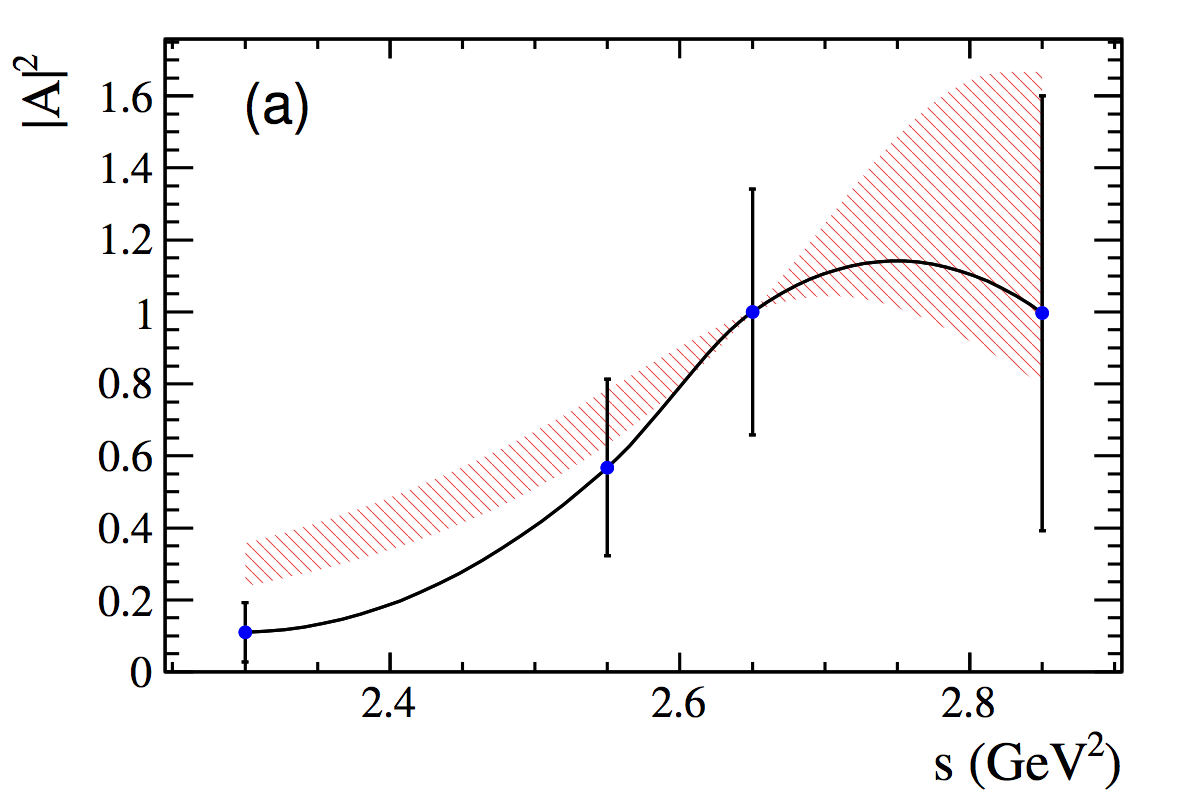
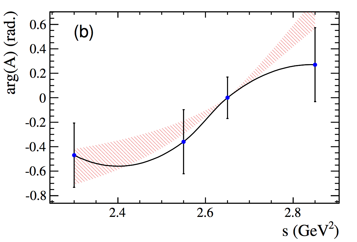
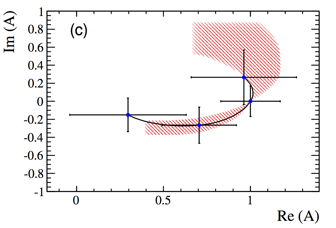
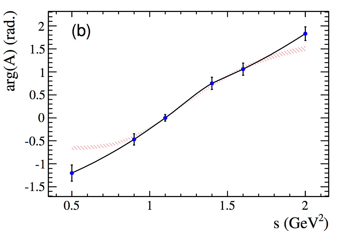
Figure 6.3: Magnitude-squared (a), phase (b) and Argand diagram (c) of the quasi-model-independent $a_{1}(1640)$ lineshape. The fitted knots are displayed as points with error bars and the black line shows the interpolated spline. The Breit-Wigner lineshape with the mass and width from the nominal fit is superimposed (red area). The latter is chosen to agree with the interpolated spline at the point $\Re(A)=1$, $\Im(A)=0$.

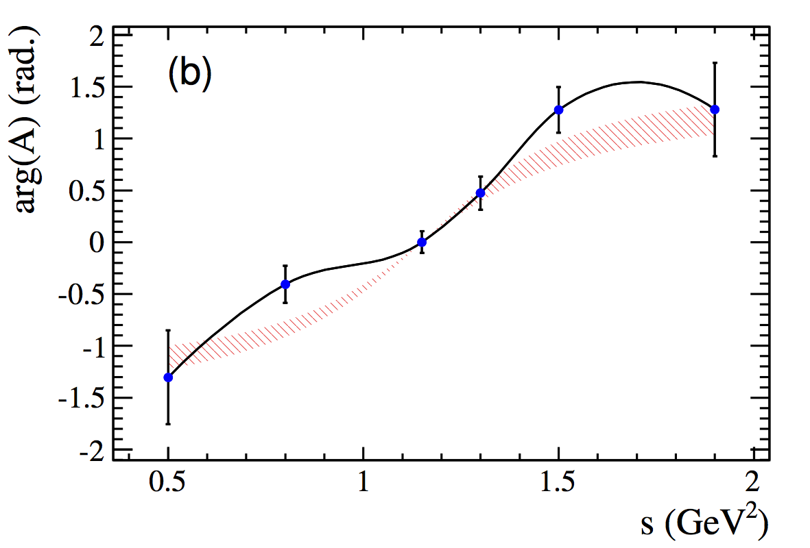
Figure 6.4: Magnitude-squared (a), phase (b) and Argand diagram (c) of the quasi-model-independent $a_{1}(1260)$ lineshape. The fitted knots are displayed as points with error bars and the black line shows the interpolated spline. The Breit-Wigner lineshape with the mass and width from the nominal fit is superimposed (red area). The latter is chosen to agree with the interpolated spline at the point $\Re(A)=1$, $\Im(A)=0$.

Figure 6.5: Magnitude-squared (a), phase (b) and Argand diagram (c) of the quasi-model-independent $\pi(1300)$ lineshape. The fitted knots are displayed as points with error bars and the black line shows the interpolated spline. The Breit-Wigner lineshape with the mass and width from the nominal fit is superimposed (red area). The latter is chosen to agree with the interpolated spline at the point $\Re(A)=1$, $\Im(A)=0$.

Since the $a_{1}(1640)^{+}$ resonance is not yet well established, we verify its resonant phase motion in a quasi-model-independent way as pioneered in Ref. [68]. For this purpose, the Breit-Wigner lineshape is replaced by a complex-valued cubic spline. The interpolated cubic spline has to pass through independent complex knots spaced in the $m^{2}({{\pi}^{+}}{{\pi}^{+}}{{\pi}^{-}})$ region around the nominal mass. The position of the knots is chosen ad-hoc. We verified on simulated experiments that with this choice a Breit-Wigner lineshape can be properly reproduced, given there is a real resonance. The fitted magnitudes and phases of the knots are shown in Fig. 6.5, where the expectations from a Breit-Wigner shape with the mass and width from the nominal fit are superimposed taking only the statistical uncertainties on the mass and width into account. The interpolated spline generally reproduces the features of the Breit-Wigner parametrization. In particular, the resulting Argand diagram shows a circular, counter-clockwise trajectory which is the expected behavior of a resonance. Note that the high-mass tail of the $a_{1}(1640)$ is outside of the phase space boundary such that it is not possible to investigate the full phase motion. Similar quasi-model-independent studies are performed for the $a_{1}(1260)$ and $\pi(1300)$ resonances as shown in Figs. 6.5 and 6.5, respectively. Since the investigated resonances are all very broad, the quasi-model-independent lineshapes can absorb statistical fluctuations in the data, especially near the phase space boundaries. Therefore, the agreement with the Breit-Wigner expectation in all cases indicates that it is qualitatively reasonable that these resonances are indeed real features of the data.

6.3 Global $C\!P$ Content Measurement

The fractional $C\!P$-even content, $F_{+}^{4\pi}$, is determined from the integral in Eq. (4.28), using the nominal model for $A^{4\pi}_{{{D}^{0}}}$ and $A^{4\pi}_{{{\kern 1.39998pt\overline{\kern-1.39998ptD}{}}{}^{0}}}$ assuming no direct $C\!P$ violation in the $D$ meson decay. The uncertainty on $F_{+}^{4\pi}$ is calculated from pseudo-experiments by randomly varying the free parameters of the amplitude fit within their measured statistical and systematic uncertainties. For each variation, $F_{+}^{4\pi}$ is redetermined, and the square root of the sample variance of these values is taken as the uncertainty. An additional systematic uncertainty is assigned by computing $F_{+}^{4\pi}$ for each of the alternative amplitude models. The standard deviation of these values is taken as the additional model uncertainty. The obtained result,

$$F_{+}^{4\pi}(\text{flavor-tagged, model-dependent})=\left[72.9\pm 0.9\mathrm{\,(stat)}\pm 1.5\mathrm{\,(syst)}\pm 1.0\;(\mathrm{model})\right]\%,$$ (6.2)

is consistent with a previous model-independent analysis of $C\!P$-tagged events [51],

$$F_{+}^{4\pi}(\text{{$C\!P$}-tagged, model-independent})=\left(73.7\pm 2.8\right)\%.$$ (6.3)

6.4 Search for Direct $C\!P$ Violation

A search for $C\!P$ violation is performed by fitting the LASSO model to the flavor-tagged ${{D}^{0}}$ and ${{\kern 1.99997pt\overline{\kern-1.99997ptD}{}}{}^{0}}$ samples. In contrast to our default fit described in Sec. 5, we now allow the amplitude coefficients for ${{D}^{0}}\rightarrow\pi^{+}\pi^{-}\pi^{+}\pi^{-}$ and ${{\kern 1.99997pt\overline{\kern-1.99997ptD}{}}{}^{0}}\rightarrow{{\pi}^{-}}{{\pi}^{+}}{{\pi}^{-}}{{\pi}^{+}}$ decays to differ, as described in Sec. 4.3.

The masses and widths of the resonances are fixed to the values obtained in the nominal fit. Possible additional biases due to this assumption are included in the systematic uncertainties which are otherwise determined as described in Sec. 8. Table 6.4 compares the resulting fit fractions for the ${{D}^{0}}$ and ${{\kern 1.99997pt\overline{\kern-1.99997ptD}{}}{}^{0}}$ decays. The sensitivity to $\mathcal{A}_{CP}^{i}$ is at the level of $4\%$ to $22\%$ depending on the decay mode. No significant $C\!P$ violation is observed for any of the amplitudes. Also, the integrated $C\!P$ asymmetry over phase space is found to be

$$\mathcal{A}^{4\pi}_{CP}=[+0.54\pm 1.04\mathrm{\,(stat)}\pm 0.51\mathrm{\,(syst)}]\%,$$ (6.4)

which is consistent with $CP$ conservation. Due to the cancellation of systematic uncertainties in asymmetry-like quantities, the only remaining source considered for the global $C\!P$ asymmetry is the tagging efficiency ratio, which is set to unity for this purpose. This nominal value of $A^{4\pi}_{CP}$ is consistent with that which can be found from the amplitude model via Eq. (4.31), $\mathcal{A}^{4\pi}_{CP}=[+0.60\pm 0.56\textrm{ (stat)}]\%$.

Table 6.4: Direct $CP$ asymmetry and significance for each component of the ${{D}^{0}}\rightarrow\pi^{+}\pi^{-}\pi^{+}\pi^{-}$ LASSO model. The first uncertainty is statistical, the second systematic and the third due to alternative models.

Decay channel	${\mathcal{A}}_{CP}^{i}$ $(\%)$	Significance ($\sigma$)
${{D}^{0}}\rightarrow{{\pi}^{-}}\,a_{1}(1260)^{+}$	$+4.7\pm 2.6\pm 4.3\pm 2.4$	$0.9$
${{D}^{0}}\rightarrow{{\pi}^{+}}\,a_{1}(1260)^{-}$	$+13.7\pm 13.8\pm 9.8\pm 5.8$	$0.8$
${{D}^{0}}\rightarrow{{\pi}^{-}}\,\pi(1300)^{+}$	$-1.6\pm 12.9\pm 5.0\pm 4.4$	$0.1$
${{D}^{0}}\rightarrow{{\pi}^{+}}\,\pi(1300)^{-}$	$-5.6\pm 11.9\pm 25.6\pm 10.3$	$0.2$
${{D}^{0}}\rightarrow{{\pi}^{-}}\,a_{1}(1640)^{+}$	$+8.6\pm 17.8\pm 16.0\pm 10.8$	$0.3$
${{D}^{0}}\rightarrow{{\pi}^{-}}\,\pi_{2}(1670)^{+}$	$+7.3\pm 15.1\pm 8.0\pm 6.6$	$0.4$
${{D}^{0}}\rightarrow\sigma\,f_{0}(1370)$	$-14.6\pm 16.5\pm 9.3\pm 1.3$	$0.8$
${{D}^{0}}\rightarrow\sigma\,\rho(770)^{0}$	$+2.5\pm 16.8\pm 13.8\pm 14.6$	$0.1$
${{D}^{0}}\rightarrow\rho(770)^{0}\,\rho(770)^{0}$	$-5.6\pm 5.0\pm 2.2\pm 1.9$	$1.0$
${{D}^{0}}\rightarrow f_{2}(1270)\,f_{2}(1270)$	$-28.3\pm 12.3\pm 18.5\pm 9.7$	$1.2$

7 ${{D}^{0}}\rightarrow K^{+}K^{-}\pi^{+}\pi^{-}$ Amplitude Analysis Results

7.1 Amplitude Model Fit Results

Table 7.1 lists the real and imaginary part of the complex amplitude coefficients $a_{i}$, along with the corresponding fit fractions. The interference fractions are given in Appendix E. Figures 7.1 and 7.2 show the distributions of selected phase space observables, which demonstrate reasonable agreement between data and the fit model. For the flavor-tagged data only, we also project into the transversity basis to demonstrate good description of the overall angular structure in Fig. 7.3: The acoplanarity angle ${\chi}$, is the angle between the two decay planes formed by the $K^{+}K^{-}$ combination and the ${{\pi}^{+}}{{\pi}^{-}}$ combination in the $D$ rest frame; boosting into the rest frames of the two-body systems defining these decay planes, the two helicity variables are defined as the cosine of the angle, ${\theta_{K^{+}}}$, of the $K^{+}$ momentum with the $D$ flight direction, and the cosine of the angle, ${\theta_{{{\pi}^{+}}}}$, of the ${{\pi}^{+}}$ momentum with the $D$ flight direction.

Table 7.1: Real and imaginary part of the complex amplitude coefficients and fit fraction of each component of the ${{D}^{0}}\rightarrow K^{+}K^{-}\pi^{+}\pi^{-}$ LASSO model. For the fit coefficients, the first quoted uncertainty is statistical, while the second arises from systematic sources. The third uncertainty in the fit fraction arises from the alternative models considered.

Decay channel	$\Re(a_{i})$	$\Im(a_{i})$	$F_{i}(\%)$
${{D}^{0}}\rightarrow K^{-}\,[K_{1}(1270)^{+}\rightarrow\pi^{+}\,K^{*}(892)^{0}]$	6.36 $\pm$ 1.24 $\pm$ 3.41	-6.86 $\pm$ 1.37 $\pm$ 3.38	5.5 $\pm$ 1.4 $\pm$ 2.7 $\pm$ 2.0
${{D}^{0}}\rightarrow K^{-}\,[K_{1}(1270)^{+}\rightarrow\pi^{+}\,K^{*}(1430)^{0}]$	34.93 $\pm$ 3.74 $\pm$ 8.39	5.66 $\pm$ 4.50 $\pm$ 6.92	6.1 $\pm$ 1.2 $\pm$ 1.3 $\pm$ 1.3
${{D}^{0}}\rightarrow K^{-}\,[K_{1}(1270)^{+}\rightarrow K^{+}\,\rho(770)^{0}]$	-17.63 $\pm$ 2.44 $\pm$ 5.26	-11.51 $\pm$ 2.27 $\pm$ 3.38	9.1 $\pm$ 1.5 $\pm$ 1.9 $\pm$ 0.1
${{D}^{0}}\rightarrow K^{+}\,[\bar{K_{1}}(1270)^{-}\rightarrow K^{-}\,\rho(770)^{0}]$	9.87 $\pm$ 1.75 $\pm$ 2.61	-12.91 $\pm$ 1.49 $\pm$ 3.82	5.4 $\pm$ 0.7 $\pm$ 1.1 $\pm$ 0.7
${{D}^{0}}\rightarrow K^{-}\,[K_{1}(1270)^{+}\rightarrow K^{+}\,\omega(782)]$	3.78 $\pm$ 3.34 $\pm$ 3.81	-9.36 $\pm$ 2.35 $\pm$ 5.87	0.6 $\pm$ 0.3 $\pm$ 0.4 $\pm$ 0.2
${{D}^{0}}\rightarrow K^{-}\,[K_{1}(1400)^{+}\rightarrow\pi^{+}\,K^{*}(892)^{0}]$	-8.08 $\pm$ 5.11 $\pm$ 8.93	-36.92 $\pm$ 4.35 $\pm$ 10.98	12.4 $\pm$ 2.6 $\pm$ 3.9 $\pm$ 5.0
${{D}^{0}}\rightarrow K^{-}\,[K^{*}(1680)^{+}\rightarrow\pi^{+}\,K^{*}(892)^{0}]$	132.69 $\pm$ 15.81 $\pm$ 27.13	-35.45 $\pm$ 19.13 $\pm$ 29.21	3.6 $\pm$ 0.8 $\pm$ 1.0 $\pm$ 0.3
${{D}^{0}}[S]\rightarrow K^{*}(892)^{0}\,\bar{K}^{*}(892)^{0}$	822.04 $\pm$ 81.84 $\pm$ 126.47	-350.52 $\pm$ 105.58 $\pm$ 234.41	4.5 $\pm$ 0.8 $\pm$ 1.1 $\pm$ 1.7
${{D}^{0}}[P]\rightarrow K^{*}(892)^{0}\,\bar{K}^{*}(892)^{0}$	-975.58 $\pm$ 115.30 $\pm$ 241.90	-476.35 $\pm$ 148.15 $\pm$ 162.11	3.6 $\pm$ 0.7 $\pm$ 1.4 $\pm$ 0.5
${{D}^{0}}[D]\rightarrow K^{*}(892)^{0}\,\bar{K}^{*}(892)^{0}$	-4786.72 $\pm$ 408.23 $\pm$ 503.72	985.18 $\pm$ 533.86 $\pm$ 941.34	4.0 $\pm$ 0.6 $\pm$ 0.7 $\pm$ 0.2
${{D}^{0}}[S]\rightarrow\phi(1020)\,\rho(770)^{0}$	5158.65 (fixed)	0.00 (fixed)	28.1 $\pm$ 1.3 $\pm$ 1.7 $\pm$ 0.3
${{D}^{0}}[P]\rightarrow\phi(1020)\,\rho(770)^{0}$	-1552.19 $\pm$ 203.06 $\pm$ 271.29	-354.72 $\pm$ 432.81 $\pm$ 531.39	1.6 $\pm$ 0.3 $\pm$ 0.6 $\pm$ 0.3
${{D}^{0}}[D]\rightarrow\phi(1020)\,\rho(770)^{0}$	5208.02 $\pm$ 685.26 $\pm$ 840.57	791.86 $\pm$ 954.63 $\pm$ 689.75	1.7 $\pm$ 0.4 $\pm$ 0.4 $\pm$ 0.2
${{D}^{0}}\rightarrow K^{*}(892)^{0}\,(K^{-}\pi^{+})_{S}$	43.52 $\pm$ 4.59 $\pm$ 9.73	-1.20 $\pm$ 5.20 $\pm$ 5.27	5.8 $\pm$ 1.2 $\pm$ 2.1 $\pm$ 0.0
${{D}^{0}}\rightarrow\phi(1020)\,(\pi^{+}\pi^{-})_{S}$	29.62 $\pm$ 7.39 $\pm$ 12.19	-54.93 $\pm$ 5.65 $\pm$ 11.92	4.0 $\pm$ 0.6 $\pm$ 1.3 $\pm$ 1.7
${{D}^{0}}\rightarrow(K^{+}K^{-})_{S}\,(\pi^{+}\pi^{-})_{S}$	0.42 $\pm$ 0.05 $\pm$ 0.10	0.49 $\pm$ 0.05 $\pm$ 0.09	11.1 $\pm$ 1.2 $\pm$ 2.1 $\pm$ 0.7
Sum			106.9 $\pm$ 4.5 $\pm$ 6.9 $\pm$ 6.1

In contrast to the treatment of the $a_{1}(1260)$ and $\pi(1300)$ substructure in the ${{D}^{0}}\rightarrow\pi^{+}\pi^{-}\pi^{+}\pi^{-}$ analysis, we do not enforce the same amplitude substructure for the $K(1270)^{+}$, $K(1400)^{+}$, $K(1680)^{+}$ decays as for $K(1270)^{-}$, $K(1400)^{-}$, $K(1680)^{-}$; this choice has historical reasons. It is re-assuring to see that the results we obtain without these constraints are consistent with what one would expect if such constraints had been applied (cf. model A in Table D.3). For the LASSO model, the $\chi^{2}/\nu$ is 1.5 with $\nu=116$, where the effective number of degrees of freedom is determined with a pseudo-experiment technique. Its value is chosen to be the one that best converts the distribution of $\chi^{2}$ values for each experiment into the standard uniform distribution. This method differs from that used in ${{D}^{0}}\rightarrow\pi^{+}\pi^{-}\pi^{+}\pi^{-}$ as the relatively small size of the data sample here would otherwise result in negative degrees of freedom.

Four alternate models are presented in Appendix D:

1. a model that requires the use of conjugate amplitudes for all present non-self-conjugate decays

2. replacing $K^{*}(1680)^{+}\rightarrow K^{*}(892)^{0}\,{{\pi}^{+}}$ with the $K^{*}(1410)^{+}\rightarrow K^{*}(892)^{0}\,{{\pi}^{+}}$ amplitude

3. replacing the flat non-resonant term with the $f_{0}(980)\,(\pi^{+}\pi^{-})_{S}$ and $f_{0}(980)\,(K^{+}K^{-})_{S}$ amplitudes

4. the model previously reported in Ref. [13]

Figure 7.1: Invariant 2-body mass distributions of ${{D}^{0}}\rightarrow K^{+}K^{-}\pi^{+}\pi^{-}$ signal candidates shown as points with error bars. The overall fit projection is shown in black, the signal in blue and the background in red. The effect of the $K^{0}_{S}$ veto can clearly be seen in the bottom right projection.

Figure 7.2: Invariant 3-body mass distributions of ${{D}^{0}}\rightarrow K^{+}K^{-}\pi^{+}\pi^{-}$ signal events shown as points with error bars. The overall fit projection is shown in black, the signal in blue and the background in red.

Figure 7.3: Angular projections of the ${{D}^{0}}\rightarrow K^{+}K^{-}\pi^{+}\pi^{-}$ fit results (black solid line) in the transversity basis, to the flavor-tagged data sample only. The signal component is shown in blue (dashed) and the background component in red (dashed).

The results between models are broadly consistent where the largest individual fit fraction corresponds to the ${{D}^{0}}\rightarrow\phi(1020)\,\rho(770)^{0}$ amplitude. We found that we cannot distinguish between the $K^{*}(1680)$ meson in our default model and the $K^{*}(1410)$ meson trialled in alternative model B. Both of these components peak outside the kinematically allowed range.

Relative to the previous analysis of the same data set [13], the most notable apparent difference in our default model is the fit fraction of the $\phi(1020)\,\rho(770)^{0}$ $S$-wave, which was 38.3% in Ref. [13], but only 28.1% in our current analysis. This is because of our modified description of the $VV$ $D$-wave. In Ref. [13], the component labeled as $D$-wave is a superposition of $D$ and $S$ waves, a choice which was motivated by the convention used in four-body amplitude analyses at the time. This led to a large interference between the components labeled as $S$ wave and $D$ wave of -15.7%. In this analysis, as we parametrize a pure $D$-wave, we find an interference fraction between the $\phi(1020)\,\rho(770)^{0}$ $S$- and $D$-waves of -3.7%. Taking these interference fractions into account, the combined $\phi(1020)\,\rho(770)^{0}$ $S$- and $D$-wave fraction of 26% is therefore consistent between both analyses. In contrast to Ref. [13], we also find a small, but significant $\phi(1020)\,\rho(770)^{0}$ $P$-wave component. Another difference in the two-resonance topology is in the $K^{*}(892)^{0}\,\bar{K}^{*}(892)^{0}$ mode, where our results indicate a significant $P$- and $D$-wave contribution, while in Ref. [13], only an $S$-wave contribution was observed. Note though, that model 6 in Ref. [13] has a $P$-wave in the $K^{*}(892)\,(K\pi)_{P}$ decay of a similar size as our $K^{*}(892)^{0}\,\bar{K}^{*}(892)^{0}$ $P$-wave. The largest differences in our results are, as might be expected, in the cascade topology, because of the significant changes we implemented to improve the description of the lineshapes of resonance decays to three-body final states. We find that the process ${{D}^{0}}\rightarrow K^{**+}\,K^{-}$, where $K^{**}$ represents any excited kaon, dominates over ${{D}^{0}}\rightarrow K^{**-}\,K^{+}$, analogous to the dominance of ${{D}^{0}}\rightarrow a_{1}(1260)^{+}\,\pi^{-}$ over ${{D}^{0}}\rightarrow a_{1}(1260)^{-}\,\pi^{+}$ decays. In Ref. [13], this was only the case for the $K(1270)\rightarrow K^{*}(890)\,\pi$ amplitude. We also observe a significant $K(1270)\rightarrow K^{*}(1430)\,\pi$ component in agreement with Ref. [14] but not with Ref. [13]. The description of this type of decay chain, with a daughter whose mean mass is outside the kinematically allowed region, benefits particularly from our improved lineshapes. As in Ref. [14], but unlike in Ref. [13], we also see a significant $K(1400)\rightarrow K^{*}(890)\,\pi$ contribution, albeit at a lower level.

7.2 Global $C\!P$ Content Measurement

Following the same approach as for ${{D}^{0}}\ \rightarrow\pi^{+}\pi^{-}\pi^{+}\pi^{-}$ decays, for the fractional $C\!P$-even content we obtain

$$F_{+}^{KK\pi\pi}=\left[75.3\pm 1.8\,(\mathrm{stat})\pm 3.3\,(\mathrm{syst})\pm 3.5\,(\mathrm{model})\right]\%,$$ (7.1)

for the nominal ${{D}^{0}}\rightarrow K^{+}K^{-}\pi^{+}\pi^{-}$ model, the first such measurement in this final state.

7.3 Search for Direct $C\!P$ Violation

Following the same approach as for ${{D}^{0}}\ \rightarrow\pi^{+}\pi^{-}\pi^{+}\pi^{-}$ decays, we measure the direct $C\!P$ violating parameters given in Table 7.2. The $C\!P$ asymmetry over phase space is found to be

$$\mathcal{A}^{KK\pi\pi}_{CP}=[+1.84\pm 1.74\mathrm{\,(stat)}\pm 0.30\mathrm{\,(syst)}]\%.$$ (7.2)

All measurements are consistent with $C\!P$ conservation.

Table 7.2: Direct $CP$ asymmetry and significance for each component of the ${{D}^{0}}\rightarrow K^{+}K^{-}\pi^{+}\pi^{-}$ LASSO model. The first uncertainty is statistical, the second systematic and the third due to alternative models.

Decay channel	${\cal A}_{CP}^{i}$ $(\%)$	Significance ($\sigma$)
${{D}^{0}}\rightarrow K^{-}\,K_{1}(1270)^{+}$	$+25.3\pm 9.7\pm 9.2\pm 8.8$	1.6
${{D}^{0}}\rightarrow K^{+}\,\bar{K_{1}}(1270)^{-}$	$-50.4\pm 12.0\pm 15.9\pm 2.4$	2.5
${{D}^{0}}\rightarrow K^{-}\,K_{1}(1400)^{+}$	$+9.2\pm 15.1\pm 20.3\pm 1.1$	0.4
${{D}^{0}}\rightarrow K^{-}\,K^{*}(1680)^{+}$	$-17.1\pm 21.8\pm 18.0\pm 4.2$	0.6
${{D}^{0}}\rightarrow K^{*}(892)^{0}\bar{K}^{*}(892)^{0}$	$-4.6\pm 9.0\pm 9.8\pm 5.7$	0.3
${{D}^{0}}\rightarrow\phi(1020)\,\rho(770)^{0}$	$+1.5\pm 4.6\pm 8.0\pm 0.5$	0.1
${{D}^{0}}\rightarrow K^{*}(892)^{0}\,(K^{-}\pi^{+})_{S}$	$-13.1\pm 17.9\pm 29.7\pm 9.4$	0.4
${{D}^{0}}\rightarrow\phi(1020)\,(\pi^{+}\pi^{-})_{S}$	$-4.0\pm 18.0\pm 44.6\pm 1.2$	0.1
${{D}^{0}}\rightarrow(K^{+}K^{-})_{S}\,(\pi^{+}\pi^{-})_{S}$	$+8.2\pm 10.9\pm 16.9\pm 2.7$	0.4

8 Systematic Uncertainties

There are three main sources of systematic uncertainties on the fit parameters to be considered; an intrinsic fit bias, as well as experimental and model-dependent uncertainties. For each four-body decay, the fit bias itself is determined from a large ensemble of MC pseudo-experiments generated from the nominal LASSO model. The mean difference between the generated and fitted parameters are taken as a systematic uncertainty.

The experimental systematic uncertainties occur due to imperfect knowledge of the yield of background events and their distribution in phase space, the wrong tag probability, and various effects on the efficiency variation over phase space. To estimate the systematic uncertainty related to the background shape that was fixed from sideband, the amplitude fit is repeated where the background parameters are allowed to vary within their statistical uncertainties. In addition, several alternative background PDFs are tested whereby each background contribution is replaced, one at a time, by a flat, non-resonant model. The largest deviations from the nominal values are assigned as systematic uncertainties. The uncertainty due to both the signal fraction and the wrong tag probabilities in the flavor-tagged samples are estimated by repeating the fit and allowing them to vary under Gaussian constraints. The signal fraction uncertainty for the $C\!P$-tagged sample is determined by fixing the fraction to unity and repeating the fit. Various assumptions made on the acceptance in the fit model are also considered. As the acceptance comes from MC, we account for differences between data and MC arising from tracking and particle identification as a function of momentum of the daughter particles. Using correction factors obtained from independent internal CLEO studies, the MC is reweighted separately for each effect and the fit to data repeated. While detector resolution can be safely ignored in ${{D}^{0}}\rightarrow\pi^{+}\pi^{-}\pi^{+}\pi^{-}$ decays, neglecting the effect of finite momentum resolution on the $\phi(1020)$ resonance in ${{D}^{0}}\rightarrow K^{+}K^{-}\pi^{+}\pi^{-}$ decays may lead to a bias. To counter this, a large number of pseudo-experiments were generated by distributing MC events that have passed full selection and weighted by the LASSO model found from data. Each experiment is then fit with the signal model where the mean difference between the generated and fitted parameters are assigned as systematic uncertainties. Finally, the integration error due to the limited size of the MC sample is of the order of $0.5\%$, so it is neglected as a source of systematic uncertainty.

Model-dependent uncertainties arise from fixed lineshape parameters and the effects of interference from Cabbibo-suppressed decays on the tag-side in the CLEO-c flavor-tagged data samples. The uncertainties due to fixed masses and widths of resonances are evaluated by varying them one-by-one within their quoted errors. In our nominal fit, the Blatt-Weisskopf radial parameter is set to $r_{\rm BW}=1.5\;(\textrm{GeV}/c)^{-1}$. As a systematic check, we set the radial parameter to zero. For the calculation of the energy-dependent widths, the partial widths into the $\pi\pi\pi$ channel are obtained using an iterative procedure described in Sec. 4.1. The systematic error of this approach is estimated by repeating the fit using the iteration previous to the final. In some cases, the energy-dependent width relies on external measurements of intermediate branching fractions. In ${{D}^{0}}\rightarrow\pi^{+}\pi^{-}\pi^{+}\pi^{-}$, their impact is studied by recalculating the width considering only decays into the $\pi\pi\pi$ ($\pi\pi$) final state for three-body (two-body) resonances. For ${{D}^{0}}\rightarrow K^{+}K^{-}\pi^{+}\pi^{-}$, the energy-dependent widths of the three-body resonances are recalculated assuming a flat phase space distribution. Similarly, the energy-dependent mass of the $a_{1}(1260)$ resonance is approximated by a constant and the resulting shifts of the fit parameters are assigned as systematic errors.

The systematic uncertainty related to interference from the tag-side arising between the CKM-favored $c\rightarrow s$ and CKM-suppressed $c\rightarrow d$ amplitudes in the final states used for flavor-tagging is accounted for by using an alternative signal PDF at the cost of two additional fit parameters as described in Ref. [13].

All systematic uncertainties are added in quadrature and summarized in Tables 8.1 and 8.2 for ${{D}^{0}}\rightarrow\pi^{+}\pi^{-}\pi^{+}\pi^{-}$ and in Tables LABEL:tab:syskkpipi and LABEL:tab:sysFractionskkpipi for ${{D}^{0}}\rightarrow K^{+}K^{-}\pi^{+}\pi^{-}$.

Table 8.1: Systematic uncertainties on the fit parameters of our nominal ${{D}^{0}}\rightarrow\pi^{+}\pi^{-}\pi^{+}\pi^{-}$ model in units of statistical standard deviations, $\sigma$. The different contributions are: 1) Blatt-Weisskopf barrier factors, 2) Masses and widths of resonances, 3) Background model, 4) Signal fraction, 5) Wrong tag fractions, 6) Tag-side interference, 7) Efficiency, 8) Fit bias, 9) Energy-dependent masses and widths.

Fit parameter	1	2	3	4	5	6	7	8	9	Total
${{D}^{0}}\rightarrow{{\pi}^{-}}\,\left[a_{1}(1260)^{+}\rightarrow{{\pi}^{+}}\,\sigma\right]\enspace\Re(a_{i})$	0.55	0.11	0.16	0.09	0.20	0.78	0.17	0.22	0.14	1.05
${{D}^{0}}\rightarrow{{\pi}^{-}}\,\left[a_{1}(1260)^{+}\rightarrow{{\pi}^{+}}\,\sigma\right]\enspace\Im(a_{i})$	1.20	0.19	0.28	0.16	0.19	0.28	0.11	0.14	0.18	1.33
${{D}^{0}}\rightarrow{{\pi}^{+}}\,a_{1}(1260)^{-}\enspace\Re(a_{i})$	0.43	1.13	0.24	0.11	0.22	0.16	0.18	0.09	0.11	1.29
${{D}^{0}}\rightarrow{{\pi}^{+}}\,a_{1}(1260)^{-}\enspace\Im(a_{i})$	0.56	0.35	0.10	0.12	0.10	0.04	0.15	0.07	0.09	0.71
${{D}^{0}}\rightarrow{{\pi}^{-}}\,\left[\pi(1300)^{+}\rightarrow{{\pi}^{+}}\,\sigma\right]\enspace\Re(a_{i})$	1.32	1.72	0.06	0.19	0.29	0.22	0.54	0.28	2.07	3.08
${{D}^{0}}\rightarrow{{\pi}^{-}}\,\left[\pi(1300)^{+}\rightarrow{{\pi}^{+}}\,\sigma\right]\enspace\Im(a_{i})$	0.12	0.53	0.20	0.17	0.25	0.22	0.08	0.09	1.51	1.67
${{D}^{0}}\rightarrow{{\pi}^{+}}\,\left[\pi(1300)^{-}\rightarrow{{\pi}^{-}}\,\sigma\right]\enspace\Re(a_{i})$	0.74	1.83	0.17	0.03	0.10	0.45	0.33	0.03	1.39	2.51
${{D}^{0}}\rightarrow{{\pi}^{+}}\,\left[\pi(1300)^{-}\rightarrow{{\pi}^{-}}\,\sigma\right]\enspace\Im(a_{i})$	0.01	1.01	0.23	0.08	0.40	0.33	0.10	0.17	2.50	2.76
${{D}^{0}}\rightarrow{{\pi}^{-}}\,\left[a_{1}(1640)^{+}[D]\rightarrow{{\pi}^{+}}\,\rho(770)^{0}\right]\enspace\Re(a_{i})$	0.85	0.44	0.09	0.11	0.06	0.90	0.14	0.34	0.33	1.39
${{D}^{0}}\rightarrow{{\pi}^{-}}\,\left[a_{1}(1640)^{+}[D]\rightarrow{{\pi}^{+}}\,\rho(770)^{0}\right]\enspace\Im(a_{i})$	0.53	0.26	0.39	0.08	0.03	0.38	0.05	0.17	0.40	0.90
${{D}^{0}}\rightarrow{{\pi}^{-}}\,\left[a_{1}(1640)^{+}\rightarrow{{\pi}^{+}}\,\sigma\right]\enspace\Re(a_{i})$	0.97	0.44	0.37	0.15	0.03	0.69	0.08	0.17	0.42	1.42
${{D}^{0}}\rightarrow{{\pi}^{-}}\,\left[a_{1}(1640)^{+}\rightarrow{{\pi}^{+}}\,\sigma\right]\enspace\Im(a_{i})$	0.45	1.23	0.19	0.13	0.23	0.80	0.12	0.01	0.35	1.61
${{D}^{0}}\rightarrow{{\pi}^{-}}\,\left[\pi_{2}(1670)^{+}\rightarrow{{\pi}^{+}}\,f_{2}(1270)\right]\enspace\Re(a_{i})$	0.70	1.57	0.44	0.02	0.16	0.24	0.11	0.13	0.41	1.84
${{D}^{0}}\rightarrow{{\pi}^{-}}\,\left[\pi_{2}(1670)^{+}\rightarrow{{\pi}^{+}}\,f_{2}(1270)\right]\enspace\Im(a_{i})$	0.21	0.38	0.14	0.08	0.06	0.89	0.15	0.07	0.16	1.03
${{D}^{0}}\rightarrow{{\pi}^{-}}\,\left[\pi_{2}(1670)^{+}\rightarrow{{\pi}^{+}}\,\sigma\right]\enspace\Re(a_{i})$	0.47	0.05	0.03	0.08	0.15	0.26	0.02	0.19	0.32	0.68
${{D}^{0}}\rightarrow{{\pi}^{-}}\,\left[\pi_{2}(1670)^{+}\rightarrow{{\pi}^{+}}\,\sigma\right]\enspace\Im(a_{i})$	0.07	1.82	0.16	0.11	0.11	0.29	0.10	0.03	0.24	1.87
${{D}^{0}}\rightarrow\sigma\,f_{0}(1370)\enspace\Re(a_{i})$	0.37	0.71	0.29	0.04	0.25	0.26	0.11	0.01	2.62	2.79
${{D}^{0}}\rightarrow\sigma\,f_{0}(1370)\enspace\Im(a_{i})$	0.85	2.24	0.15	0.04	0.18	0.28	0.53	0.10	1.09	2.71
${{D}^{0}}\rightarrow\sigma\,\rho(770)^{0}\enspace\Re(a_{i})$	0.01	0.86	0.22	0.07	0.07	0.49	0.07	0.20	0.24	1.06
${{D}^{0}}\rightarrow\sigma\,\rho(770)^{0}\enspace\Im(a_{i})$	0.81	0.99	0.18	0.09	0.11	1.05	0.19	0.05	0.66	1.81
${{D}^{0}}[S]\rightarrow\rho(770)^{0}\,\rho(770)^{0}\enspace\Re(a_{i})$	0.25	1.05	0.06	0.07	0.13	1.11	0.13	0.15	0.40	1.62
${{D}^{0}}[S]\rightarrow\rho(770)^{0}\,\rho(770)^{0}\enspace\Im(a_{i})$	1.24	0.35	0.25	0.05	0.08	0.26	0.13	0.05	0.03	1.35
${{D}^{0}}[P]\rightarrow\rho(770)^{0}\,\rho(770)^{0}\enspace\Re(a_{i})$	0.17	0.97	0.16	0.08	0.18	0.31	0.02	0.11	0.32	1.11
${{D}^{0}}[P]\rightarrow\rho(770)^{0}\,\rho(770)^{0}\enspace\Im(a_{i})$	0.18	2.08	0.10	0.11	0.20	1.32	0.09	0.17	0.15	2.50
${{D}^{0}}[D]\rightarrow\rho(770)^{0}\,\rho(770)^{0}\enspace\Re(a_{i})$	0.45	1.33	0.05	0.08	0.09	0.43	0.04	0.01	0.31	1.51
${{D}^{0}}[D]\rightarrow\rho(770)^{0}\,\rho(770)^{0}\enspace\Im(a_{i})$	0.05	1.60	0.34	0.07	0.03	0.78	0.19	0.20	0.05	1.83
${{D}^{0}}\rightarrow f_{2}(1270)\,f_{2}(1270)\enspace\Re(a_{i})$	0.67	0.52	0.23	0.10	0.22	0.37	0.10	0.24	0.17	1.03
${{D}^{0}}\rightarrow f_{2}(1270)\,f_{2}(1270)\enspace\Im(a_{i})$	0.50	1.11	0.19	0.02	0.07	0.02	0.06	0.04	0.15	1.24
$m_{a_{1}(1260)}$	1.31	1.15	0.14	0.04	0.14	0.10	0.13	0.15	0.52	1.85
$\Gamma_{a_{1}(1260)}$	0.10	0.48	0.04	0.04	0.01	0.04	0.13	0.03	0.88	1.03
$m_{\pi(1300)}$	0.75	0.78	0.19	0.15	0.36	0.10	0.39	0.12	1.90	2.26
$\Gamma_{\pi(1300)}$	0.11	0.82	0.06	0.02	0.25	0.05	0.16	0.17	1.27	1.55
$m_{a_{1}(1640)}$	0.64	0.45	0.06	0.05	0.13	0.03	0.07	0.22	0.37	0.89
$\Gamma_{a_{1}(1640)}$	0.54	0.21	0.12	0.09	0.05	0.04	0.05	0.38	0.07	0.61

Table 8.2: Systematic uncertainties on the fit fractions from our nominal ${{D}^{0}}\rightarrow\pi^{+}\pi^{-}\pi^{+}\pi^{-}$ model in units of statistical standard deviations, $\sigma$. The different contributions are: 1) Blatt-Weisskopf barrier factors, 2) Masses and widths of resonances, 3) Background model, 4) Signal fraction, 5) Wrong tag fractions, 6) Tag-side interference, 7) Efficiency, 8) Fit bias, 9) Energy-dependent masses and widths.

Decay channel	1	2	3	4	5	6	7	8	9	Total
${{D}^{0}}\rightarrow{{\pi}^{-}}\,\left[a_{1}(1260)^{+}\rightarrow{{\pi}^{+}}\,\rho(770)^{0}\right]$	0.19	1.32	0.18	0.15	0.18	0.17	0.08	0.08	0.15	1.39
${{D}^{0}}\rightarrow{{\pi}^{-}}\,\left[a_{1}(1260)^{+}\rightarrow{{\pi}^{+}}\,\sigma\right]$	1.09	0.76	0.22	0.13	0.17	0.54	0.18	0.03	0.25	1.50
${{D}^{0}}\rightarrow{{\pi}^{+}}\,\left[a_{1}(1260)^{-}\rightarrow{{\pi}^{-}}\,\rho(770)^{0}\right]$	0.55	0.56	0.19	0.06	0.11	0.10	0.13	0.09	0.06	0.83
${{D}^{0}}\rightarrow{{\pi}^{+}}\,\left[a_{1}(1260)^{-}\rightarrow{{\pi}^{-}}\,\sigma\right]$	0.14	0.24	0.24	0.11	0.20	0.21	0.13	0.06	0.06	0.50
${{D}^{0}}\rightarrow{{\pi}^{-}}\,\left[\pi(1300)^{+}\rightarrow{{\pi}^{+}}\,\sigma\right]$	0.55	1.25	0.26	0.05	0.20	0.51	0.40	0.07	0.62	1.67
${{D}^{0}}\rightarrow{{\pi}^{+}}\,\left[\pi(1300)^{-}\rightarrow{{\pi}^{-}}\,\sigma\right]$	0.08	1.34	0.26	0.09	0.32	1.01	0.11	0.06	2.85	3.33
${{D}^{0}}\rightarrow{{\pi}^{-}}\,\left[a_{1}(1640)^{+}[D]\rightarrow{{\pi}^{+}}\,\rho(770)^{0}\right]$	0.68	0.55	0.14	0.11	0.09	1.08	0.22	0.09	0.47	1.50
${{D}^{0}}\rightarrow{{\pi}^{-}}\,\left[a_{1}(1640)^{+}\rightarrow{{\pi}^{+}}\,\sigma\right]$	0.65	1.07	0.12	0.15	0.20	0.89	0.13	0.02	0.13	1.57
${{D}^{0}}\rightarrow{{\pi}^{-}}\,\left[\pi_{2}(1670)^{+}\rightarrow{{\pi}^{+}}\,f_{2}(1270)\right]$	0.18	0.79	0.19	0.01	0.06	0.79	0.09	0.06	0.18	1.17
${{D}^{0}}\rightarrow{{\pi}^{-}}\,\left[\pi_{2}(1670)^{+}\rightarrow{{\pi}^{+}}\,\sigma\right]$	0.35	1.23	0.12	0.07	0.08	0.31	0.06	0.02	0.14	1.33
${{D}^{0}}\rightarrow\sigma\,f_{0}(1370)$	0.70	1.79	0.09	0.10	0.15	0.81	0.52	0.03	0.88	2.33
${{D}^{0}}\rightarrow\sigma\,\rho(770)^{0}$	0.58	0.22	0.14	0.06	0.04	0.83	0.07	0.05	0.58	1.20
${{D}^{0}}[S]\rightarrow\rho(770)^{0}\,\rho(770)^{0}$	1.12	0.93	0.27	0.05	0.15	0.46	0.12	0.07	0.17	1.57
${{D}^{0}}[P]\rightarrow\rho(770)^{0}\,\rho(770)^{0}$	0.09	1.84	0.24	0.03	0.02	2.60	0.13	0.26	0.13	3.20
${{D}^{0}}[D]\rightarrow\rho(770)^{0}\,\rho(770)^{0}$	0.74	1.19	0.09	0.07	0.06	0.90	0.17	0.07	0.26	1.70
${{D}^{0}}\rightarrow f_{2}(1270)\,f_{2}(1270)$	0.17	0.48	0.11	0.07	0.16	0.17	0.04	0.11	0.16	0.60

Table 8.3: Systematic uncertainties on the fit parameters of our nominal ${{D}^{0}}\rightarrow K^{+}K^{-}\pi^{+}\pi^{-}$ model in units of statistical standard deviations, $\sigma$. The different contributions are: 1) Blatt-Weisskopf barrier factors, 2) Masses and widths of resonances, 3) $C\!P$-tagged signal fraction, 4) Flavor-tagged background model, 5) Flavor-tagged signal fractions, 6) Mistag rates, 7) Tag-side interference, 8) Efficiency, 9) Fit bias, 10) Detector resolution, 11) Energy-dependent masses and widths.

Fit parameter	1	2	3	4	5	6	7	8	9	10	11	Total
${{D}^{0}}\rightarrow K^{-}\,\left[K_{1}(1270)^{+}\rightarrow\pi^{+}\,K^{*}(892)^{0}\right]\enspace\Re(a_{i})$	0.732	2.126	0.190	0.199	0.019	0.001	0.101	0.376	0.090	0.211	1.505	2.757
${{D}^{0}}\rightarrow K^{-}\,\left[K_{1}(1270)^{+}\rightarrow\pi^{+}\,K^{*}(892)^{0}\right]\enspace\Im(a_{i})$	0.331	2.396	0.207	0.147	0.087	0.001	0.064	0.300	0.040	0.233	0.054	2.465
${{D}^{0}}\rightarrow K^{-}\,\left[K_{1}(1270)^{+}\rightarrow\pi^{+}\,K^{*}(1430)^{0}\right]\enspace\Re(a_{i})$	0.493	2.050	0.244	0.277	0.005	0.001	0.212	0.090	0.274	0.434	0.344	2.240
${{D}^{0}}\rightarrow K^{-}\,\left[K_{1}(1270)^{+}\rightarrow\pi^{+}\,K^{*}(1430)^{0}\right]\enspace\Im(a_{i})$	0.295	1.125	0.196	0.147	0.024	0.002	0.842	0.060	0.190	0.085	0.445	1.538
${{D}^{0}}\rightarrow K^{-}\,\left[K_{1}(1270)^{+}\rightarrow K^{+}\,\rho(770)^{0}\right]\enspace\Re(a_{i})$	0.470	2.011	0.199	0.154	0.009	0.002	0.207	0.063	0.292	0.283	0.332	2.157
${{D}^{0}}\rightarrow K^{-}\,\left[K_{1}(1270)^{+}\rightarrow K^{+}\,\rho(770)^{0}\right]\enspace\Im(a_{i})$	0.014	1.127	0.165	0.181	0.027	0.001	0.466	0.215	0.042	0.021	0.780	1.485
${{D}^{0}}\rightarrow K^{+}\,\left[K_{1}(1270)^{-}\rightarrow K^{-}\,\rho(770)^{0}\right]\enspace\Re(a_{i})$	0.560	0.972	0.160	0.169	0.172	0.001	0.512	0.139	0.100	0.226	0.746	1.497
${{D}^{0}}\rightarrow K^{+}\,\left[K_{1}(1270)^{-}\rightarrow K^{-}\,\rho(770)^{0}\right]\enspace\Im(a_{i})$	1.008	2.125	0.213	0.298	0.123	0.000	0.346	0.216	0.306	0.178	0.773	2.564
${{D}^{0}}\rightarrow K^{-}\,\left[K_{1}(1270)^{+}\rightarrow K^{+}\,\omega(782)\right]\enspace\Re(a_{i})$	0.549	0.713	0.149	0.216	0.024	0.001	0.165	0.025	0.157	0.087	0.605	1.142
${{D}^{0}}\rightarrow K^{-}\,\left[K_{1}(1270)^{+}\rightarrow K^{+}\,\omega(782)\right]\enspace\Im(a_{i})$	0.030	1.506	0.097	0.033	0.032	0.000	0.714	0.274	0.178	0.387	1.785	2.497
${{D}^{0}}\rightarrow K^{-}\,\left[K_{1}(1400)^{+}\rightarrow\pi^{+}\,K^{*}(892)^{0}\right]\enspace\Re(a_{i})$	0.228	1.587	0.292	0.176	0.132	0.000	0.221	0.180	0.057	0.169	0.489	1.748
${{D}^{0}}\rightarrow K^{-}\,\left[K_{1}(1400)^{+}\rightarrow\pi^{+}\,K^{*}(892)^{0}\right]\enspace\Im(a_{i})$	0.090	1.880	0.101	0.146	0.047	0.001	0.821	0.151	0.312	0.082	1.409	2.522
${{D}^{0}}\rightarrow K^{-}\,\left[K^{*}(1680)^{+}\rightarrow\pi^{+}\,K^{*}(892)^{0}\right]\enspace\Re(a_{i})$	0.636	0.732	0.639	0.095	0.106	0.000	0.989	0.246	0.010	0.567	0.467	1.716
${{D}^{0}}\rightarrow K^{-}\,\left[K^{*}(1680)^{+}\rightarrow\pi^{+}\,K^{*}(892)^{0}\right]\enspace\Im(a_{i})$	0.423	0.716	0.254	0.136	0.066	0.003	0.051	0.060	0.043	0.301	1.206	1.527
${{D}^{0}}[S]\rightarrow K^{*}(892)^{0}\bar{K}^{*}(892)^{0}\enspace\Re(a_{i})$	0.044	0.547	0.218	0.177	0.054	0.002	1.006	0.221	0.357	0.146	0.892	1.545
${{D}^{0}}[S]\rightarrow K^{*}(892)^{0}\bar{K}^{*}(892)^{0}\enspace\Im(a_{i})$	0.536	1.151	0.169	0.135	0.026	0.001	0.237	0.028	0.091	0.019	1.790	2.220
${{D}^{0}}[P]\rightarrow K^{*}(892)^{0}\bar{K}^{*}(892)^{0}\enspace\Re(a_{i})$	0.575	0.437	0.171	0.261	0.016	0.001	1.909	0.198	0.015	0.236	0.213	2.098
${{D}^{0}}[P]\rightarrow K^{*}(892)^{0}\bar{K}^{*}(892)^{0}\enspace\Im(a_{i})$	0.518	0.480	0.412	0.205	0.011	0.001	0.401	0.154	0.226	0.020	0.501	1.094
${{D}^{0}}[D]\rightarrow K^{*}(892)^{0}\bar{K}^{*}(892)^{0}\enspace\Re(a_{i})$	0.863	0.252	0.636	0.273	0.068	0.000	0.055	0.141	0.069	0.430	0.132	1.234
${{D}^{0}}[D]\rightarrow K^{*}(892)^{0}\bar{K}^{*}(892)^{0}\enspace\Im(a_{i})$	0.445	0.595	0.162	0.228	0.085	0.002	0.453	0.154	0.013	0.162	1.489	1.763
${{D}^{0}}[P]\rightarrow\phi(1020)\rho(770)^{0}\enspace\Re(a_{i})$	0.695	0.161	0.145	0.435	0.009	0.003	1.006	0.023	0.128	0.132	0.139	1.336
${{D}^{0}}[P]\rightarrow\phi(1020)\rho(770)^{0}\enspace\Im(a_{i})$	0.243	0.289	0.209	0.793	0.014	0.000	0.085	0.099	0.112	0.322	0.747	1.228
${{D}^{0}}[D]\rightarrow\phi(1020)\rho(770)^{0}\enspace\Re(a_{i})$	0.709	0.100	0.750	0.179	0.013	0.001	0.040	0.185	0.009	0.399	0.449	1.227
${{D}^{0}}[D]\rightarrow\phi(1020)\rho(770)^{0}\enspace\Im(a_{i})$	0.064	0.227	0.524	0.349	0.002	0.001	0.053	0.023	0.152	0.107	0.178	0.723
${{D}^{0}}\rightarrow K^{*}(892)^{0}(K^{-}\pi^{+})_{S}\enspace\Re(a_{i})$	0.762	1.161	0.464	0.114	0.146	0.002	1.357	0.134	0.309	0.233	0.548	2.119
${{D}^{0}}\rightarrow K^{*}(892)^{0}(K^{-}\pi^{+})_{S}\enspace\Im(a_{i})$	0.693	0.358	0.162	0.145	0.118	0.001	0.070	0.105	0.228	0.194	0.502	1.013
${{D}^{0}}\rightarrow\phi(1020)(\pi^{+}\pi^{-})_{S}\enspace\Re(a_{i})$	0.132	0.209	0.210	0.247	0.013	0.001	0.670	0.107	0.446	0.657	1.208	1.648
${{D}^{0}}\rightarrow\phi(1020)(\pi^{+}\pi^{-})_{S}\enspace\Im(a_{i})$	0.685	0.194	0.302	0.755	0.087	0.001	1.720	0.057	0.292	0.402	0.266	2.111
${{D}^{0}}\rightarrow(K^{+}K^{-})_{S}(\pi^{+}\pi^{-})_{S}\enspace\Re(a_{i})$	1.163	0.519	0.201	0.499	0.049	0.001	0.255	0.169	0.044	0.087	1.301	1.926
${{D}^{0}}\rightarrow(K^{+}K^{-})_{S}(\pi^{+}\pi^{-})_{S}\enspace\Im(a_{i})$	0.999	0.525	0.202	0.606	0.319	0.001	1.223	0.291	0.020	0.038	0.531	1.910

Table 8.4: Systematic uncertainties on the fit fractions from our nominal ${{D}^{0}}\rightarrow K^{+}K^{-}\pi^{+}\pi^{-}$ model in units of statistical standard deviations, $\sigma$. The different contributions are: 1) Blatt-Weisskopf barrier factors, 2) Masses and widths of resonances, 3) $C\!P$-tagged signal fraction, 4) Flavor-tagged background model, 5) Flavor-tagged signal fractions, 6) Mistag rates, 7) Tag-side interference, 8) Efficiency, 9) Fit bias, 10) Detector resolution, 11) Energy-dependent masses and widths.

Decay channel	1	2	3	4	5	6	7	8	9	10	11	Total
${{D}^{0}}\rightarrow K^{-}\,\left[K_{1}(1270)^{+}\rightarrow\pi^{+}\,K^{*}(892)^{0}\right]$	0.224	0.960	0.084	0.071	0.028	0.000	0.034	0.140	0.027	0.094	0.406	1.087
${{D}^{0}}\rightarrow K^{-}\,\left[K_{1}(1270)^{+}\rightarrow\pi^{+}\,K^{*}(1430)^{0}\right]$	0.436	1.812	0.217	0.245	0.006	0.001	0.236	0.080	0.243	0.382	0.312	1.987
${{D}^{0}}\rightarrow K^{-}\,\left[K_{1}(1270)^{+}\rightarrow K^{+}\,\rho(770)^{0}\right]$	0.319	1.443	0.151	0.129	0.013	0.001	0.239	0.099	0.199	0.192	0.394	1.588
${{D}^{0}}\rightarrow K^{+}\,\left[{K_{1}}(1270)^{-}\rightarrow K^{-}\,\rho(770)^{0}\right]$	0.495	1.009	0.113	0.147	0.087	0.000	0.252	0.110	0.140	0.118	0.449	1.271
${{D}^{0}}\rightarrow K^{-}\,\left[K_{1}(1270)^{+}\rightarrow K^{+}\,\omega(782)\right]$	0.178	0.879	0.073	0.072	0.020	0.000	0.406	0.155	0.112	0.220	1.025	1.454
${{D}^{0}}\rightarrow K^{-}\,\left[K_{1}(1400)^{+}\rightarrow\pi^{+}\,K^{*}(892)^{0}\right]$	0.063	1.125	0.074	0.089	0.034	0.001	0.481	0.092	0.183	0.054	0.827	1.498
${{D}^{0}}\rightarrow K^{-}\,\left[K^{*}(1680)^{+}\rightarrow\pi^{+}\,K^{*}(892)^{0}\right]$	0.420	0.496	0.416	0.068	0.070	0.001	0.639	0.159	0.011	0.371	0.393	1.153
${{D}^{0}}[S]\rightarrow K^{*}(892)^{0}\bar{K}^{*}(892)^{0}$	0.224	0.630	0.178	0.145	0.042	0.002	0.764	0.167	0.271	0.110	1.000	1.483
${{D}^{0}}[P]\rightarrow K^{*}(892)^{0}\bar{K}^{*}(892)^{0}$	0.528	0.424	0.248	0.233	0.014	0.001	1.540	0.176	0.114	0.189	0.304	1.766
${{D}^{0}}[D]\rightarrow K^{*}(892)^{0}\bar{K}^{*}(892)^{0}$	1.182	0.405	0.865	0.379	0.097	0.001	0.181	0.199	0.094	0.586	0.572	1.793
${{D}^{0}}[S]\rightarrow\phi(1020)\rho(770)^{0}$	1.190	0.265	0.832	0.622	0.021	0.003	0.807	0.211	0.137	0.524	0.712	2.015
${{D}^{0}}[P]\rightarrow\phi(1020)\rho(770)^{0}$	0.635	0.193	0.159	0.524	0.010	0.003	0.906	0.048	0.125	0.185	0.351	1.318
${{D}^{0}}[D]\rightarrow\phi(1020)\rho(770)^{0}$	0.620	0.097	0.663	0.169	0.011	0.001	0.036	0.162	0.029	0.349	0.394	1.080
${{D}^{0}}\rightarrow K^{*}(892)^{0}(K^{-}\pi^{+})_{S}$	0.328	0.500	0.200	0.049	0.063	0.001	0.584	0.058	0.133	0.100	0.236	0.912
${{D}^{0}}\rightarrow\phi(1020)(\pi^{+}\pi^{-})_{S}$	0.606	0.214	0.295	0.679	0.077	0.001	1.564	0.083	0.376	0.538	0.783	2.113
${{D}^{0}}\rightarrow(K^{+}K^{-})_{S}(\pi^{+}\pi^{-})_{S}$	0.946	0.458	0.177	0.490	0.206	0.001	0.797	0.212	0.029	0.058	0.851	1.681

9 Conclusion

The first amplitude analysis of flavor-tagged ${{D}^{0}}\rightarrow\pi^{+}\pi^{-}\pi^{+}\pi^{-}$ decays has been presented based on CLEO-c data. Due to the large amount of possible intermediate resonance components, a model-building procedure has been applied which balances the fit quality against the number of free fit parameters. The prominent contribution is found to be the $a_{1}(1260)$ resonance in the decay modes $a_{1}(1260)\rightarrow\rho(770)^{0}\,\pi$ and $a_{1}(1260)\rightarrow\sigma\,\pi$. Along with the $a_{1}(1260)$, further cascade decays involving the resonances $\pi(1300)$ and $a_{1}(1640)$ are also seen. The masses and widths of these resonances are determined using an advanced lineshape parametrization taking into account the resonant three-pion substructure. The resonant phase motion of these states has been verified by means of a quasi-model-independent study. In addition to these cascade topologies, there is a significant contribution from the quasi-two-body decays ${{D}^{0}}\rightarrow\rho(770)^{0}\,\rho(770)^{0}$ and ${{D}^{0}}\rightarrow\sigma\,f_{0}(1370)$. The $C\!P$-even fraction of the decay ${{D}^{0}}\rightarrow\pi^{+}\pi^{-}\pi^{+}\pi^{-}$ as predicted by the amplitude model is consistent with a previous model-independent study. The amplitude model has also been used to search for $C\!P$ violation in ${{D}^{0}}\rightarrow\pi^{+}\pi^{-}\pi^{+}\pi^{-}$ decays, where no $C\!P$ violation among the amplitudes is observed within the given precision of a few percent.

Moreover, the amplitude analysis of ${D}\rightarrow K^{+}K^{-}\pi^{+}\pi^{-}$ decays performed by CLEO [13] has been revisited by applying the significantly improved formalism presented in this paper, using decays obtained from CLEO II.V, CLEO III, and CLEO-c data. The largest components are the processes ${{D}^{0}}\rightarrow\phi(1020)\,\rho(770)^{0}$, ${{D}^{0}}\rightarrow K_{1}(1270)^{+}\,K^{-}$ and ${{D}^{0}}\rightarrow K(1400)^{+}\,K^{-}$, which together account for over half of the ${{D}^{0}}\rightarrow K^{+}K^{-}\pi^{+}\pi^{-}$ decay rate. The fractional $C\!P$-even content is measured for the first time and a search for $C\!P$ asymmetries in the amplitude components yields no evidence for $C\!P$ violation.

In addition to shedding light on the dynamics of ${{D}^{0}}\rightarrow h^{+}h^{-}\pi^{+}\pi^{-}$ decays, these results are expected to provide important input for a determination of the $C\!P$-violating phase $\gamma$ $(\phi_{3})$ in $B^{-}\rightarrow D{{K}^{-}}$ decays.

Appendices

Appendix A Energy-Dependent Widths

Figure A.1: Energy-dependent width for the $f_{0}(1370)$ (a) and $f_{2}(1270)$ (b) resonances. The total width is shown in black (solid), while the partial widths into the channels $\pi\pi$, $\pi\pi\pi\pi$ and $KK+\eta\eta$ are shown in blue (dashed), red (dotted) and green (dashed-dotted), respectively.

Figure A.2: Final iteration of the energy-dependent width for the $\pi(1300)$ (a) and $a_{1}(1640)$ (b) resonances.

Figure A.3: Energy-dependent width for the $\pi_{2}(1670)$ resonance. The total width is shown in black (solid), while the partial widths into the channels $\pi\pi\pi$, $\omega\rho(770)$ and $K\bar{K}\pi$ are shown in blue (dashed), red (dotted) and green (dashed-dotted), respectively.

Figure A.4: Energy-dependent width for the $K_{1}(1270)$ (a) and $K_{1}(1400)$ (b) resonances. The total width is shown in black (solid), while the partial widths into the channels $K\pi\pi$ and $K\omega$ are shown in blue (dashed) and red (dotted), respectively.

Figure A.5: Energy-dependent width for the $K^{*}(1410)$ (a) and $K^{*}(1680)$ (b) resonances. The total width is shown in black (solid), while the partial widths into the channels $K\pi\pi$ and $K\pi$ are shown in blue (dashed) and red (dotted), respectively.

Appendix B Spin Amplitudes

The spin factors used for $D\rightarrow P_{1}\,P_{2}\,P_{3}\,P_{4}$ decays are given in Table B.1. To fix our phase convention, we give the exact matching of the particles $P_{1}$, $P_{2}$, $P_{3}$, and $P_{4}$ in the spin factor definition to the final state particles in specific decay chains in Tables B.2 and B.3.

Table B.1: Spin factors for all topologies considered in this analysis. In the decay chains, $S$, $P$, $V$, $A$, $T$ and $PT$ stand for scalar, pseudoscalar, vector, axial vector, tensor and pseudotensor, respectively. If no angular momentum is specified, the lowest angular momentum state compatible with angular momentum conservation and, where appropriate, parity conservation, is used.

Number	Decay chain	Spin amplitude
1	$D\rightarrow(P\,P_{1})$, $P\rightarrow(S\,P_{2})$, $S\rightarrow(P_{3}\,P_{4})$	$1$
2	$D\rightarrow(P\,P_{1})$, $P\rightarrow(V\,P_{2})$, $V\rightarrow(P_{3}\,P_{4})$	$L_{(1)\alpha}(P)\,\,L_{(1)}^{\alpha}(V)$
3	$D\rightarrow(A\,P_{1})$, $A\rightarrow(V\,P_{2})$, $V\rightarrow(P_{3}\,P_{4})$	$L_{(1)\alpha}(D)\,P_{(1)}^{\alpha\beta}(A)\,L_{(1)\beta}(V)$
4	$D\rightarrow(A\,P_{1})$, $A[D]\rightarrow(P_{2}\,V)$, $V\rightarrow(P_{3}\,P_{4})$	$L_{(1)\alpha}(D)\,L_{(2)}^{\alpha\beta}(A)\,L_{(1)\beta}(V)$
5	$D\rightarrow(A\,P_{1})$, $A\rightarrow(S\,P_{2})$, $S\rightarrow(P_{3}\,P_{4})$	$L_{(1)\alpha}(D)\,L_{(1)}^{\alpha}(A)$
6	$D\rightarrow(A\,P_{1})$, $A\rightarrow(T\,P_{2})$, $T\rightarrow(P_{3}\,P_{4})$	$L_{(1)\alpha}(D)\,L_{(1)\beta}(A)\,L_{(2)}^{\alpha\beta}(T)$
7	$D\rightarrow(V_{1}\,P_{1})$, $V_{1}\rightarrow(V_{2}\,P_{2})$, $V_{2}\rightarrow(P_{3}\,P_{4})$	$L_{(1)\mu}(D)\,P_{(1)}^{\mu\alpha}(V_{1})\,\epsilon_{\alpha\beta\gamma\delta}\,L_{(1)}^{\beta}(V_{1})\,p_{V_{1}}^{\gamma}\,L_{(1)}^{\delta}(V_{2})$
8	$D\rightarrow(PT\,P_{1})$, $PT\rightarrow(V\,P_{2})$, $V\rightarrow(P_{3}\,P_{4})$	$L_{(2)\alpha\beta}(D)\,P_{(2)}^{\alpha\beta\gamma\delta}(PT)\,L_{(1)\gamma}(PT)\,L_{(1)\delta}(V)$
9	$D\rightarrow(PT\,P_{1})$, $PT\rightarrow(S\,P_{2})$, $S\rightarrow(P_{3}\,P_{4})$	$L_{(2)\alpha\beta}(D)\,L_{(2)}(PT)^{\alpha\beta}$
10	$D\rightarrow(PT\,P_{1})$, $PT\rightarrow(T\,P_{2})$, $T\rightarrow(P_{3}\,P_{4})$	$L_{(2)\alpha\beta}(D)\,P_{(2)}^{\alpha\beta\gamma\delta}(PT)\,L_{(2)\gamma\delta}(T)$
11	$D\rightarrow(T\,P_{1})$, $T\rightarrow(V\,P_{2})$, $V\rightarrow(P_{3}\,P_{4})$	$L_{(2)\mu\nu}(D)\,P_{(2)}^{\mu\nu\rho\alpha}(T)\,\epsilon_{\alpha\beta\gamma\delta}\,L_{(2)\rho}^{\beta}(T)\,p_{T}^{\gamma}\,P_{(1)}^{\delta\sigma}(T)\,L_{(1)\sigma}(V)$
12	$D\rightarrow(T_{1}\,P_{1})$, $T_{1}\rightarrow(T_{2}\,P_{2})$, $T_{2}\rightarrow(P_{3}\,P_{4})$	$L_{(2)\mu\nu}(D)\,P_{(2)}^{\mu\nu\rho\alpha}(T_{1})\,\epsilon_{\alpha\beta\gamma\delta}\,L_{(1)}^{\beta}(T_{1})\,p_{T_{1}}^{\gamma}\,L_{(2)\rho}^{\delta}(T_{2})$
13	$D\rightarrow(S_{1}\,S_{2})$, $S_{1}\rightarrow(P_{1}\,P_{2})$, $S_{2}\rightarrow(P_{3}\,P_{4})$	$1$
14	$D\rightarrow(V\,S)$, $V\rightarrow(P_{1}\,P_{2})$, $S\rightarrow(P_{3}\,P_{4})$	$L_{(1)\alpha}(D)\,L_{(1)}^{\alpha}(V)$
15	$D\rightarrow(V_{1}\,V_{2})$, $V_{1}\rightarrow(P_{1}\,P_{2})$, $V_{2}\rightarrow(P_{3}\,P_{4})$	$L_{(1)\alpha}(V_{1})\,L_{(1)}^{\alpha}(V_{2})$
16	$D[P]\rightarrow(V_{1}\,V_{2})$, $V_{1}\rightarrow(P_{1}\,P_{2})$, $V_{2}\rightarrow(P_{3}\,P_{4})$	$\epsilon_{\alpha\beta\gamma\delta}\,L_{(1)}^{\alpha}(D)\,L_{(1)}^{\beta}(V_{1})\,L_{(1)}^{\gamma}(V_{2})\,p_{D}^{\delta}$
17	$D[D]\rightarrow(V_{1}\,V_{2})$, $V_{1}\rightarrow(P_{1}\,P_{2})$, $V_{2}\rightarrow(P_{3}\,P_{4})$	$L_{(2)\alpha\beta}(D)\,L_{(1)}^{\alpha}(V_{1})\,L_{(1)}^{\beta}(V_{2})$
18	$D\rightarrow(T\,S)$, $T\rightarrow(P_{1}\,P_{2})$, $S\rightarrow(P_{3}\,P_{4})$	$L_{(2)\alpha\beta}(D)\,L_{(2)}^{\alpha\beta}(T)$
19	$D\rightarrow(V\,T)$, $T\rightarrow(P_{1}\,P_{2})$, $V\rightarrow(P_{3}\,P_{4})$	$L_{(1)\alpha}(D)\,L_{(2)}^{\alpha\beta}(T)\,L_{(1)\beta}(V)$
20	$D[D]\rightarrow(T\,V)$, $T\rightarrow(P_{1}\,P_{2})$, $V\rightarrow(P_{3}\,P_{4})$	$\epsilon_{\alpha\beta\delta\gamma}\,L_{2}^{\alpha\mu}(D)\,L_{2\mu}^{\beta}\,L_{(1)}^{\gamma}(V)\,p_{D}^{\delta}$
21	$D\rightarrow(T_{1}\,T_{2})$, $T_{1}\rightarrow(P_{1}\,P_{2})$, $T_{2}\rightarrow(P_{3}\,P_{4})$	$L_{(2)\alpha\beta}(T_{1})\,L_{(2)}^{\alpha\beta}(T_{2})$
22	$D[P]\rightarrow(T_{1}\,T_{2})$, $T_{1}\rightarrow(P_{1}\,P_{2})$, $T_{2}\rightarrow(P_{3}\,P_{4})$	$\epsilon_{\alpha\beta\gamma\delta}\,L_{(1)}^{\alpha}(D)\,L_{(2)}^{\beta\mu}(T_{1})\,L_{(2)\mu}^{\gamma}(T_{2})\,p_{D}^{\delta}$
23	$D[D]\rightarrow(T_{1}\,T_{2})$, $T_{1}\rightarrow(P_{1}\,P_{2})$, $T_{2}\rightarrow(P_{3}\,P_{4})$	$L_{(2)\alpha\beta}(D)\,L_{(2)}^{\alpha\gamma}(T_{1})\,L_{(2)\gamma}^{\beta}(T_{2})$

Table B.2: Spin factors used for the decay chains included in the ${{D}^{0}}\rightarrow\pi^{+}\pi^{-}\pi^{+}\pi^{-}$ LASSO model, including the particle numbering scheme. The second column refers to the spin factors as numbered in Table B.1, and the particles $P_{1}$, $P_{2}$, $P_{3}$, and $P_{4}$ refer to those defined in Table B.1.

Decay channel	Spin factor number	$P_{1}$	$P_{2}$	$P_{3}$	$P_{4}$
${{D}^{0}}\rightarrow{{\pi}^{-}}\,\left[a_{1}(1260)^{+}\rightarrow{{\pi}^{+}}\,\rho(770)^{0}\right]$	3	${\pi}^{-}$	${\pi}^{+}$	${\pi}^{+}$	${\pi}^{-}$
${{D}^{0}}\rightarrow{{\pi}^{-}}\,\left[a_{1}(1260)^{+}\rightarrow{{\pi}^{+}}\,\sigma\right]$	5	${\pi}^{-}$	${\pi}^{+}$	${\pi}^{+}$	${\pi}^{-}$
${{D}^{0}}\rightarrow{{\pi}^{+}}\,\left[a_{1}(1260)^{-}\rightarrow{{\pi}^{-}}\,\rho(770)^{0}\right]$	3	${\pi}^{+}$	${\pi}^{-}$	${\pi}^{-}$	${\pi}^{+}$
${{D}^{0}}\rightarrow{{\pi}^{+}}\,\left[a_{1}(1260)^{-}\rightarrow{{\pi}^{-}}\,\sigma\right]$	5	${\pi}^{+}$	${\pi}^{-}$	${\pi}^{-}$	${\pi}^{+}$
${{D}^{0}}\rightarrow{{\pi}^{-}}\,\left[\pi(1300)^{+}\rightarrow{{\pi}^{+}}\,\sigma\right]$	1	${\pi}^{-}$	${\pi}^{+}$	${\pi}^{+}$	${\pi}^{-}$
${{D}^{0}}\rightarrow{{\pi}^{+}}\,\left[\pi(1300)^{-}\rightarrow{{\pi}^{-}}\,\sigma\right]$	1	${\pi}^{+}$	${\pi}^{-}$	${\pi}^{-}$	${\pi}^{+}$
${{D}^{0}}\rightarrow{{\pi}^{-}}\,\left[a_{1}(1640)^{+}[D]\rightarrow{{\pi}^{+}}\,\rho(770)^{0}\right]$	4	${\pi}^{-}$	${\pi}^{+}$	${\pi}^{+}$	${\pi}^{-}$
${{D}^{0}}\rightarrow{{\pi}^{-}}\,\left[a_{1}(1640)^{+}\rightarrow{{\pi}^{+}}\,\sigma\right]$	5	${\pi}^{-}$	${\pi}^{+}$	${\pi}^{+}$	${\pi}^{-}$
${{D}^{0}}\rightarrow{{\pi}^{-}}\,\left[\pi_{2}(1670)^{+}\rightarrow{{\pi}^{+}}\,f_{2}(1270)\right]$	10	${\pi}^{-}$	${\pi}^{+}$	${\pi}^{+}$	${\pi}^{-}$
${{D}^{0}}\rightarrow{{\pi}^{-}}\,\left[\pi_{2}(1670)^{+}\rightarrow{{\pi}^{+}}\,\sigma\right]$	9	${\pi}^{-}$	${\pi}^{+}$	${\pi}^{+}$	${\pi}^{-}$
${{D}^{0}}\rightarrow\sigma\,f_{0}(1370)$	13	${\pi}^{+}$	${\pi}^{-}$	${\pi}^{+}$	${\pi}^{-}$
${{D}^{0}}\rightarrow\sigma\,\rho(770)^{0}$	14	${\pi}^{+}$	${\pi}^{-}$	${\pi}^{+}$	${\pi}^{-}$
${{D}^{0}}[S]\rightarrow\rho(770)^{0}\,\rho(770)^{0}$	15	${\pi}^{+}$	${\pi}^{-}$	${\pi}^{+}$	${\pi}^{-}$
${{D}^{0}}[P]\rightarrow\rho(770)^{0}\,\rho(770)^{0}$	16	${\pi}^{+}$	${\pi}^{-}$	${\pi}^{+}$	${\pi}^{-}$
${{D}^{0}}[D]\rightarrow\rho(770)^{0}\,\rho(770)^{0}$	17	${\pi}^{+}$	${\pi}^{-}$	${\pi}^{+}$	${\pi}^{-}$
${{D}^{0}}\rightarrow f_{2}(1270)\,f_{2}(1270)$	21	${\pi}^{+}$	${\pi}^{-}$	${\pi}^{+}$	${\pi}^{-}$

Table B.3: Spin factors used for the decay chains included in the ${{D}^{0}}\rightarrow K^{+}K^{-}\pi^{+}\pi^{-}$ LASSO model, including the particle numbering scheme. The second column refers to the spin factors as numbered in Table B.1, and the particles $P_{1}$, $P_{2}$, $P_{3}$, and $P_{4}$ refer to those defined in Table B.1.

Decay channel	Spin factor number	$P_{1}$	$P_{2}$	$P_{3}$	$P_{4}$
${{D}^{0}}\rightarrow K^{-}\,[K_{1}(1270)^{+}\rightarrow\pi^{+}\,K^{*}(892)^{0}]$	3	${K}^{-}$	${\pi}^{+}$	${K}^{+}$	${\pi}^{-}$
${{D}^{0}}\rightarrow K^{-}\,[K_{1}(1270)^{+}\rightarrow\pi^{+}\,K^{*}(1430)^{0}]$	5	${K}^{-}$	${\pi}^{+}$	${K}^{+}$	${\pi}^{-}$
${{D}^{0}}\rightarrow K^{-}\,[K_{1}(1270)^{+}\rightarrow K^{+}\,\rho(770)^{0}]$	3	${K}^{-}$	${K}^{+}$	${\pi}^{+}$	${\pi}^{-}$
${{D}^{0}}\rightarrow K^{+}\,[\bar{K_{1}}(1270)^{-}\rightarrow K^{-}\,\rho(770)^{0}]$	3	${K}^{+}$	${K}^{-}$	${\pi}^{-}$	${\pi}^{+}$
${{D}^{0}}\rightarrow K^{-}\,[K_{1}(1270)^{+}\rightarrow K^{+}\,\omega(782)]$	3	${K}^{-}$	${K}^{+}$	${\pi}^{+}$	${\pi}^{-}$
${{D}^{0}}\rightarrow K^{-}\,[K_{1}(1400)^{+}\rightarrow\pi^{+}\,K^{*}(892)^{0}]$	3	${K}^{-}$	${\pi}^{+}$	${K}^{+}$	${\pi}^{-}$
${{D}^{0}}\rightarrow K^{-}\,[K^{*}(1680)^{+}\rightarrow\pi^{+}\,K^{*}(892)^{0}]$	7	${K}^{-}$	${\pi}^{+}$	${K}^{+}$	${\pi}^{-}$
${{D}^{0}}[S]\rightarrow K^{*}(892)^{0}\,\bar{K}^{*}(892)^{0}$	15	${K}^{+}$	${\pi}^{-}$	${K}^{-}$	${\pi}^{+}$
${{D}^{0}}[P]\rightarrow K^{*}(892)^{0}\,\bar{K}^{*}(892)^{0}$	16	${K}^{+}$	${\pi}^{-}$	${K}^{-}$	${\pi}^{+}$
${{D}^{0}}[D]\rightarrow K^{*}(892)^{0}\,\bar{K}^{*}(892)^{0}$	17	${K}^{+}$	${\pi}^{-}$	${K}^{-}$	${\pi}^{+}$
${{D}^{0}}[S]\rightarrow\phi(1020)\,\rho(770)^{0}$	15	${K}^{+}$	${K}^{-}$	${\pi}^{+}$	${\pi}^{-}$
${{D}^{0}}[P]\rightarrow\phi(1020)\,\rho(770)^{0}$	16	${K}^{+}$	${K}^{-}$	${\pi}^{+}$	${\pi}^{-}$
${{D}^{0}}[D]\rightarrow\phi(1020)\,\rho(770)^{0}$	17	${K}^{+}$	${K}^{-}$	${\pi}^{+}$	${\pi}^{-}$
${{D}^{0}}\rightarrow K^{*}(892)^{0}\,(K^{-}\pi^{+})_{S}$	14	${K}^{+}$	${\pi}^{-}$	${K}^{-}$	${\pi}^{+}$
${{D}^{0}}\rightarrow\phi(1020)\,(\pi^{+}\pi^{-})_{S}$	14	${K}^{+}$	${K}^{-}$	${\pi}^{+}$	${\pi}^{-}$
${{D}^{0}}\rightarrow(K^{+}K^{-})_{S}\,(\pi^{+}\pi^{-})_{S}$	13	${K}^{+}$	${K}^{-}$	${\pi}^{+}$	${\pi}^{-}$

Appendix C Considered Decay Chains

The various decay channels considered in the model building are listed in Tables C.1 and C.2.

Table C.1: Decays considered in ${{D}^{0}}\rightarrow\pi^{+}\pi^{-}\pi^{+}\pi^{-}$ LASSO model building. For cascade non-self-conjugate channels, the conjugate partner is implied.

Decay channel
${{D}^{0}}\rightarrow{{\pi}^{-}}\,\left[a_{1}(1260)^{+}\rightarrow{{\pi}^{+}}\,\sigma\right]$
${{D}^{0}}\rightarrow{{\pi}^{-}}\,\left[a_{1}(1260)^{+}[S,D]\rightarrow{{\pi}^{+}}\,\rho(770)^{0}\right]$
${{D}^{0}}\rightarrow{{\pi}^{-}}\,\left[a_{1}(1260)^{+}\rightarrow{{\pi}^{+}}\,f_{0}(980)\right]$
${{D}^{0}}\rightarrow{{\pi}^{-}}\,\left[a_{1}(1260)^{+}\rightarrow{{\pi}^{+}}\,f_{2}(1270)\right]$
${{D}^{0}}\rightarrow{{\pi}^{-}}\,\left[a_{1}(1260)^{+}\rightarrow{{\pi}^{+}}\,f_{0}(1370)\right]$
${{D}^{0}}\rightarrow{{\pi}^{-}}\,\left[a_{1}(1260)^{+}[S,D]\rightarrow{{\pi}^{+}}\,\rho(1450)^{0}\right]$
${{D}^{0}}\rightarrow{{\pi}^{-}}\,\left[\pi(1300)^{+}\rightarrow{{\pi}^{+}}\,\sigma\right]$
${{D}^{0}}\rightarrow{{\pi}^{-}}\,\left[\pi(1300)^{+}\rightarrow{{\pi}^{+}}\,\rho(770)^{0}\right]$
${{D}^{0}}\rightarrow{{\pi}^{-}}\,\left[\pi(1300)^{+}\rightarrow{{\pi}^{+}}\,({{\pi}^{+}}{{\pi}^{-}})_{P}\right]$
${{D}^{0}}\rightarrow{{\pi}^{-}}\,\left[a_{2}(1320)^{+}\rightarrow{{\pi}^{+}}\,\rho(770)^{0}\right]$
${{D}^{0}}\rightarrow{{\pi}^{-}}\,\left[a_{2}(1320)^{+}\rightarrow{{\pi}^{+}}\,f_{2}(1270)\right]$
${{D}^{0}}\rightarrow{{\pi}^{-}}\,\left[a_{1}(1420)^{+}\rightarrow{{\pi}^{+}}\,f_{0}(980)\right]$
${{D}^{0}}\rightarrow{{\pi}^{-}}\,\left[\pi_{1}(1600)^{+}\rightarrow{{\pi}^{+}}\,\rho(770)^{0}\right]$
${{D}^{0}}\rightarrow{{\pi}^{-}}\,\left[a_{1}(1640)^{+}\rightarrow{{\pi}^{+}}\,\sigma\right]$
${{D}^{0}}\rightarrow{{\pi}^{-}}\,\left[a_{1}(1640)^{+}[S,D]\rightarrow{{\pi}^{+}}\,\rho(770)^{0}\right]$
${{D}^{0}}\rightarrow{{\pi}^{-}}\,\left[a_{1}(1640)^{+}\rightarrow{{\pi}^{+}}\,f_{2}(1270)\right]$
${{D}^{0}}\rightarrow{{\pi}^{-}}\,\left[\pi_{2}(1670)^{+}\rightarrow{{\pi}^{+}}\,\sigma\right]$
${{D}^{0}}\rightarrow{{\pi}^{-}}\,\left[\pi_{2}(1670)^{+}\rightarrow{{\pi}^{+}}\,\rho(770)^{0}\right]$
${{D}^{0}}\rightarrow{{\pi}^{-}}\,\left[\pi_{2}(1670)^{+}\rightarrow{{\pi}^{+}}\,f_{2}(1270)\right]$
${{D}^{0}}\rightarrow(\pi\,\pi)_{S}\,(\pi\,\pi)_{S}$
${{D}^{0}}\rightarrow\sigma\,(\pi\,\pi)_{S}$
${{D}^{0}}\rightarrow\sigma\,\sigma$
${{D}^{0}}\rightarrow\sigma\,f_{0}(980)$
${{D}^{0}}\rightarrow\sigma\,f_{0}(1370)$
${{D}^{0}}\rightarrow f_{0}(980)\,f_{0}(980)$
${{D}^{0}}\rightarrow f_{0}(1370)\,f_{0}(1370)$
${{D}^{0}}\rightarrow\rho(770)^{0}\,\sigma$
${{D}^{0}}\rightarrow\rho(770)^{0}\,f_{0}(980)$
${{D}^{0}}\rightarrow\rho(770)^{0}\,f_{0}(1370)$
${{D}^{0}}\rightarrow\rho(1450)^{0}\,\sigma$
${{D}^{0}}[S,P,D]\rightarrow(\pi\,\pi)_{P}\,(\pi\,\pi)_{P}$
${{D}^{0}}[S,P,D]\rightarrow\rho(770)^{0}\,(\pi\,\pi)_{P}$
${{D}^{0}}[S,P,D]\rightarrow\rho(770)^{0}\,\rho(770)^{0}$
${{D}^{0}}[S,P,D]\rightarrow\rho(770)^{0}\,\omega(782)^{0}$
${{D}^{0}}[S,P,D]\rightarrow\omega(782)^{0}\,\omega(782)^{0}$
${{D}^{0}}[S,P,D]\rightarrow\rho(1450)^{0}\,(\pi\,\pi)_{P}$
${{D}^{0}}[S,P,D]\rightarrow\rho(1450)^{0}\,\rho(1450)^{0}$
${{D}^{0}}\rightarrow f_{2}(1270)\,\sigma$
${{D}^{0}}\rightarrow f_{2}(1270)\,f_{0}(980)$
${{D}^{0}}[P,D]\rightarrow f_{2}(1270)\,\rho(770)^{0}$
${{D}^{0}}[S,P,D]\rightarrow f_{2}(1270)\,f_{2}(1270)$

Table C.2: Decays considered in ${{D}^{0}}\rightarrow K^{+}K^{-}\pi^{+}\pi^{-}$ LASSO model building. For cascade non-self-conjugate channels, the conjugate partner is implied.

Decay channel
${{D}^{0}}\rightarrow K^{-}\,[K^{*}(1410)^{+}\rightarrow\pi^{+}\,K^{*}(892)^{0}]$
${{D}^{0}}\rightarrow K^{-}\,[K_{1}(1270)^{+}[S,D]\rightarrow\pi^{+}\,K^{*}(892)^{0}]$
${{D}^{0}}\rightarrow K^{-}\,[K_{1}(1270)^{+}[S,D]\rightarrow\pi^{+}\,K^{*}(1430)^{0}]$
${{D}^{0}}\rightarrow K^{-}\,[K_{1}(1270)^{+}[S,D]\rightarrow K^{+}\,\rho(770)^{0}]$
${{D}^{0}}\rightarrow K^{-}\,[K_{1}(1270)^{+}[S,D]\rightarrow K^{+}\,\omega(782)]$
${{D}^{0}}\rightarrow K^{-}\,[K_{1}(1400)^{+}[S,D]\rightarrow\pi^{+}\,K^{*}(892)^{0}]$
${{D}^{0}}\rightarrow K^{-}\,[K_{2}^{*}(1430)^{+}\rightarrow\pi^{+}\,K^{*}(892)^{0}]$
${{D}^{0}}\rightarrow K^{-}\,[K_{2}^{*}(1430)^{+}\rightarrow K^{+}\,\rho(770)^{0}]$
${{D}^{0}}\rightarrow K^{-}\,[K^{*}(1680)^{+}\rightarrow\pi^{+}\,K^{*}(892)^{0}]$
${{D}^{0}}\rightarrow K^{-}\,[K^{*}(1680)^{+}\rightarrow K^{+}\,\rho(770)^{0}]$
${{D}^{0}}[S,P,D]\rightarrow K^{*}(892)^{0}\,\bar{K}^{*}(892)^{0}$
${{D}^{0}}[S,P,D]\rightarrow\phi(1020)\,\rho(770)^{0}$
${{D}^{0}}\rightarrow\phi(1020)\,\omega(782)$
${{D}^{0}}[P,D]\rightarrow f_{2}(1270)^{0}\,\phi(1020)$
${{D}^{0}}\rightarrow\rho(770)^{0}\,(K^{+}K^{-})_{S}$
${{D}^{0}}[S,P,D]\rightarrow\rho(770)^{0}\,(K^{+}K^{-})_{P}$
${{D}^{0}}\rightarrow K^{*}(892)^{0}\,(K^{-}\pi^{+})_{S}$
${{D}^{0}}[S,P,D]\rightarrow K^{*}(892)^{0}\,(K^{-}\pi^{+})_{P}$
${{D}^{0}}\rightarrow\phi(1020)\,(\pi^{+}\pi^{-})_{S}$
${{D}^{0}}[S,P,D]\rightarrow\phi(1020)\,(\pi^{+}\pi^{-})_{P}$
${{D}^{0}}\rightarrow f_{0}(980)\,(\pi^{+}\pi^{-})_{S}$
${{D}^{0}}\rightarrow f_{0}(980)\,(K^{+}K^{-})_{S}$
${{D}^{0}}\rightarrow(K^{+}K^{-})_{S}\,(\pi^{+}\pi^{-})_{S}$

Appendix D Alternative Fit Models

The fit fractions and $\chi^{2}$ values of the baseline and several alternative models are summarized in Tables D.1-D.3.

Table D.1: Fit fractions in percent for each component of specific alternative models for ${D}^{0}$ $\rightarrow$ $\pi^{+}\pi^{-}\pi^{+}\pi^{-}$. Resonance parameters, $F_{+}^{4\pi}$ and $\chi^{2}/\nu$ are also given. The uncertainties are statistical only.

Decay mode	Extended	No $\pi(1300)$	No $a_{1}(1640)$	FOCUS
${{D}^{0}}\rightarrow{{\pi}^{-}}\,\left[a_{1}(1260)^{+}\rightarrow{{\pi}^{+}}\,\rho(770)^{0}\right]$	$37.3\pm 1.9$	$41.0\pm 2.7$	$36.7\pm 2.9$	$38.2\pm 2.8$
${{D}^{0}}\rightarrow{{\pi}^{-}}\,\left[a_{1}(1260)^{+}[D]\rightarrow{{\pi}^{+}}\,\rho(770)^{0}\right]$	-	-	$2.6\pm 0.5$	$7.0\pm 1.2$
${{D}^{0}}\rightarrow{{\pi}^{-}}\,\left[a_{1}(1260)^{+}\rightarrow{{\pi}^{+}}\,\sigma\right]$	$8.1\pm 1.2$	$5.5\pm 0.7$	$5.1\pm 0.8$	$6.6\pm 0.9$
${{D}^{0}}\rightarrow{{\pi}^{+}}\,\left[a_{1}(1260)^{-}\rightarrow{{\pi}^{-}}\,\rho(770)^{0}\right]$	$2.1\pm 0.4$	$3.0\pm 0.5$	$1.0\pm 0.2$	-
${{D}^{0}}\rightarrow{{\pi}^{+}}\,\left[a_{1}(1260)^{-}[D]\rightarrow{{\pi}^{-}}\,\rho(770)^{0}\right]$	-	-	$0.07\pm 0.04$	-
${{D}^{0}}\rightarrow{{\pi}^{+}}\,\left[a_{1}(1260)^{-}\rightarrow{{\pi}^{-}}\,\sigma\right]$	$0.5\pm 0.2$	$0.4\pm 0.2$	$0.14\pm 0.06$	-
${{D}^{0}}\rightarrow{{\pi}^{-}}\,\left[\pi(1300)^{+}\rightarrow{{\pi}^{+}}\,\sigma\right]$	$8.6\pm 0.9$	-	$10.7\pm 1.8$	-
${{D}^{0}}\rightarrow{{\pi}^{+}}\,\left[\pi(1300)^{-}\rightarrow{{\pi}^{-}}\,\sigma\right]$	$5.0\pm 0.7$	-	$2.8\pm 0.8$	-
${{D}^{0}}\rightarrow{{\pi}^{-}}\,\left[a_{1}(1640)^{+}[D]\rightarrow{{\pi}^{+}}\,\rho(770)^{0}\right]$	$2.9\pm 0.4$	$6.5\pm 0.8$	-	-
${{D}^{0}}\rightarrow{{\pi}^{-}}\,\left[a_{1}(1640)^{+}\rightarrow{{\pi}^{+}}\,\sigma\right]$	$3.0\pm 0.7$	-	-	-
${{D}^{0}}\rightarrow{{\pi}^{-}}\,\left[a_{1}(1640)^{+}\rightarrow{{\pi}^{+}}\,f_{2}(1270)\right]$	-	$2.1\pm 0.8$	-	-
${{D}^{0}}\rightarrow{{\pi}^{+}}\,\left[a_{1}(1640)^{-}[D]\rightarrow{{\pi}^{-}}\,\rho(770)^{0}\right]$	$1.0\pm 0.6$	-	-	-
${{D}^{0}}\rightarrow{{\pi}^{+}}\,\left[a_{1}(1640)^{-}\rightarrow{{\pi}^{-}}\,\sigma\right]$	$1.1\pm 0.6$	-	-	-
${{D}^{0}}\rightarrow{{\pi}^{-}}\,\left[\pi_{2}(1670)^{+}\rightarrow{{\pi}^{+}}\,f_{2}(1270)\right]$	$0.8\pm 0.3$	$2.6\pm 0.7$	$3.4\pm 0.8$	-
${{D}^{0}}\rightarrow{{\pi}^{-}}\,\left[\pi_{2}(1670)^{+}\rightarrow{{\pi}^{+}}\,\sigma\right]$	$3.3\pm 0.5$	$3.4\pm 0.6$	$1.0\pm 0.3$	-
${{D}^{0}}\rightarrow{{\pi}^{+}}\,\left[\pi_{2}(1670)^{-}\rightarrow{{\pi}^{-}}\,f_{2}(1270)\right]$	$0.3\pm 0.2$	-	-	-
${{D}^{0}}\rightarrow{{\pi}^{+}}\,\left[\pi_{2}(1670)^{-}\rightarrow{{\pi}^{-}}\,\sigma\right]$	$1.3\pm 0.6$	-	-	-
${{D}^{0}}\rightarrow\sigma\,(\pi\,\pi)_{S}$	-	-	-	$24.7\pm 2.7$
${{D}^{0}}\rightarrow\sigma\,f_{0}(1370)$	$26.1\pm 1.8$	$9.4\pm 1.0$	$28.4\pm 2.8$	-
${{D}^{0}}\rightarrow f_{0}(980)\,(\pi\,\pi)_{S}$	-	-	-	$4.6\pm 1.1$
${{D}^{0}}\rightarrow\sigma\,\rho(770)^{0}$	$10.6\pm 1.1$	$6.3\pm 0.9$	$7.4\pm 1.2$	-
${{D}^{0}}[S]\rightarrow\rho(770)^{0}\,\rho(770)^{0}$	$0.9\pm 0.3$	$3.2\pm 0.7$	$0.8\pm 0.4$	$5.0\pm 1.4$
${{D}^{0}}[P]\rightarrow\rho(770)^{0}\,\rho(770)^{0}$	$6.8\pm 0.5$	$6.5\pm 0.6$	$6.9\pm 0.5$	$6.3\pm 0.7$
${{D}^{0}}[D]\rightarrow\rho(770)^{0}\,\rho(770)^{0}$	$13.2\pm 1.0$	$3.7\pm 0.8$	$11.8\pm 1.6$	$3.2\pm 0.8$
${{D}^{0}}\rightarrow f_{2}(1270)\,(\pi\,\pi)_{S}$	-	-	-	$2.4\pm 0.6$
${{D}^{0}}\rightarrow f_{2}(1270)\,\sigma$	-	$1.1\pm 0.7$	$1.4\pm 0.4$	-
${{D}^{0}}\rightarrow f_{2}(1270)\,f_{0}(980)$	-	$4.6\pm 1.0$	-	-
${{D}^{0}}\rightarrow f_{2}(1270)\,f_{2}(1270)$	$2.1\pm 0.4$	$7.9\pm 1.7$	$4.0\pm 0.8$	-
Sum	$135\pm 4$	$107\pm 4$	$124\pm 5$	$98\pm 4$
$m_{a_{1}(1260)}\,(\mathrm{\,Me\kern-0.70004ptV}/c^{2})$	$1225\pm 10$	$1225\pm 9$	$1230\pm 9$	$1304\pm 14$
$\Gamma_{a_{1}(1260)}\,(\mathrm{\,Me\kern-0.70004ptV})$	$442\pm 26$	$460\pm 30$	$421\pm 26$	$529\pm 38$
$m_{\pi(1300)}\,(\mathrm{\,Me\kern-0.70004ptV}/c^{2})$	$1093\pm 21$	-	$1135\pm 22$	-
$\Gamma_{\pi(1300)}\,(\mathrm{\,Me\kern-0.70004ptV})$	$314\pm 36$	-	$308\pm 36$	-
$m_{a_{1}(1640)}\,(\mathrm{\,Me\kern-0.70004ptV}/c^{2})$	$1710\pm 20$	$1727\pm 20$	-	-
$\Gamma_{a_{1}(1640)}\,(\mathrm{\,Me\kern-0.70004ptV})$	$201\pm 38$	$141\pm 45$	-	-
$\chi^{2}/\nu$	1.52	1.79	1.55	2.36
$\nu$	217	223	223	237
$F_{+}^{4\pi}\,(\%)$	$70.8\pm 0.9$	$70.8\pm 0.9$	$72.6\pm 0.9$	$61.7\pm 0.8$

Table D.2: Fit fractions in percent for each component of various alternative models for ${{D}^{0}}\rightarrow\pi^{+}\pi^{-}\pi^{+}\pi^{-}$ based on fit quality. Resonance parameters, $F_{+}^{4\pi}$ and $\chi^{2}/\nu$ are also given. The uncertainties are statistical only.

Decay mode	Alt. 1	Alt. 2	Alt. 3	Alt. 4	Alt. 5
${{D}^{0}}\rightarrow{{\pi}^{-}}\,\left[a_{1}(1260)^{+}\rightarrow{{\pi}^{+}}\,\rho(770)^{0}\right]$	$37.1\pm 2.3$	${38.3\pm 2.4}$	$35.2\pm 2.6$	$38.4\pm 2.5$	$35.7\pm 2.7$
${{D}^{0}}\rightarrow{{\pi}^{-}}\,\left[a_{1}(1260)^{+}\rightarrow{{\pi}^{+}}\,\sigma\right]$	$11.3\pm 1.0$	$9.8\pm 1.2$	$9.4\pm 1.2$	$11.6\pm 1.4$	$11.4\pm 1.7$
${{D}^{0}}\rightarrow{{\pi}^{+}}\,\left[a_{1}(1260)^{-}\rightarrow{{\pi}^{-}}\,\rho(770)^{0}\right]$	$2.1\pm 0.5$	$3.3\pm 0.6$	$3.7\pm 0.7$	$3.1\pm 0.6$	$4.1\pm 0.7$
${{D}^{0}}\rightarrow{{\pi}^{+}}\,\left[a_{1}(1260)^{-}\rightarrow{{\pi}^{-}}\,\sigma\right]$	$0.6\pm 0.2$	$0.9\pm 0.2$	$1.0\pm 0.3$	$0.9\pm 0.2$	$1.3\pm 0.3$
${{D}^{0}}\rightarrow{{\pi}^{-}}\,\left[\pi(1300)^{+}\rightarrow{{\pi}^{+}}\,({{\pi}^{+}}\,{{\pi}^{-}})_{P}\right]$	-	-	-	-	$6.4\pm 1.3$
${{D}^{0}}\rightarrow{{\pi}^{-}}\,\left[\pi(1300)^{+}\rightarrow{{\pi}^{+}}\,\sigma\right]$	$8.1\pm 1.0$	$8.6\pm 1.4$	$6.0\pm 1.0$	$7.7\pm 1.6$	$4.3\pm 1.1$
${{D}^{0}}\rightarrow{{\pi}^{+}}\,\left[\pi(1300)^{-}\rightarrow{{\pi}^{-}}\,({{\pi}^{+}}\,{{\pi}^{-}})_{P}\right]$	-	-	-	-	$2.5\pm 0.5$
${{D}^{0}}\rightarrow{{\pi}^{+}}\,\left[\pi(1300)^{-}\rightarrow{{\pi}^{-}}\,\sigma\right]$	$4.3\pm 0.9$	$4.0\pm 1.5$	$6.8\pm 1.6$	$4.9\pm 1.6$	$1.7\pm 0.4$
${{D}^{0}}\rightarrow{{\pi}^{-}}\,\left[a_{1}(1640)^{+}[D]\rightarrow{{\pi}^{+}}\,\rho(770)^{0}\right]$	$2.7\pm 0.9$	$4.5\pm 1.5$	$3.9\pm 1.6$	$5.2\pm 1.1$	$3.7\pm 1.8$
${{D}^{0}}\rightarrow{{\pi}^{-}}\,\left[a_{1}(1640)^{+}\rightarrow{{\pi}^{+}}\,\sigma\right]$	$3.2\pm 1.3$	$1.4\pm 0.5$	$2.4\pm 1.0$	$3.0\pm 0.9$	$1.2\pm 0.7$
${{D}^{0}}\rightarrow{{\pi}^{-}}\,\left[\pi_{2}(1670)^{+}\rightarrow{{\pi}^{+}}\,f_{2}(1270)\right]$	$1.8\pm 0.5$	$0.6\pm 0.2$	$1.2\pm 0.4$	$1.7\pm 0.5$	$1.6\pm 0.4$
${{D}^{0}}\rightarrow{{\pi}^{-}}\,\left[\pi_{2}(1670)^{+}\rightarrow{{\pi}^{+}}\,\rho(770)^{0}\right]$	$2.7\pm 0.5$	-	-	-	-
${{D}^{0}}\rightarrow{{\pi}^{-}}\,\left[\pi_{2}(1670)^{+}\rightarrow{{\pi}^{+}}\,\sigma\right]$	$2.1\pm 0.4$	$3.9\pm 0.6$	$3.3\pm 0.6$	$3.8\pm 0.6$	$3.5\pm 0.6$
${{D}^{0}}\rightarrow\sigma\,f_{0}(1370)$	$20.7\pm 2.2$	$19.3\pm 2.4$	$21.3\pm 2.4$	$21.8\pm 2.5$	$20.4\pm 2.1$
${{D}^{0}}\rightarrow\sigma\,\rho(770)^{0}$	$5.5\pm 1.0$	$8.7\pm 1.2$	$8.7\pm 1.4$	-	$4.8\pm 1.2$
${{D}^{0}}\rightarrow f_{0}(980)\,\rho(770)^{0}$	-	-	$3.6\pm 0.8$	-	-
${{D}^{0}}\rightarrow f_{0}(1370)\,\rho(770)^{0}$	-	-	-	$5.8\pm 1.0$	-
${{D}^{0}}[S]\rightarrow\rho(770)^{0}\,\rho(770)^{0}$	-	$1.5\pm 0.4$	$0.8\pm 0.4$	$1.2\pm 0.4$	$0.9\pm 0.4$
${{D}^{0}}[P]\rightarrow\rho(770)^{0}\,\rho(770)^{0}$	$7.3\pm 0.5$	$6.8\pm 0.5$	$6.9\pm 0.5$	$6.8\pm 0.5$	$6.4\pm 0.5$
${{D}^{0}}[D]\rightarrow\rho(770)^{0}\,\rho(770)^{0}$	$10.4\pm 0.9$	$8.3\pm 1.0$	$11.4\pm 1.4$	$10.9\pm 1.2$	$16.0\pm 2.1$
${{D}^{0}}\rightarrow f_{2}(1270)\,f_{2}(1270)$	$2.5\pm 0.5$	-	$1.2\pm 0.3$	$1.4\pm 0.4$	$1.1\pm 0.3$
Sum	$122\pm 4$	$120\pm 3$	$127\pm 4$	$128\pm 4$	$127\pm 6$
$m_{a_{1}(1260)}\,(\mathrm{\,Me\kern-0.70004ptV}/c^{2})$	$1198\pm 8$	$1220\pm 8$	$1213\pm 9$	$1215\pm 8$	$1231\pm 9$
$\Gamma_{a_{1}(1260)}\,(\mathrm{\,Me\kern-0.70004ptV})$	$429\pm 24$	$408\pm 23$	$434\pm 24$	$420\pm 24$	$459\pm 25$
$m_{\pi(1300)}\,(\mathrm{\,Me\kern-0.70004ptV}/c^{2})$	$1110\pm 17$	$1079\pm 25$	$1075\pm 22$	$1077\pm 36$	$1180\pm 15$
$\Gamma_{\pi(1300)}\,(\mathrm{\,Me\kern-0.70004ptV})$	$314\pm 39$	$347\pm 40$	$330\pm 39$	$377\pm 41$	$297\pm 36$
$m_{a_{1}(1640)}\,(\mathrm{\,Me\kern-0.70004ptV}/c^{2})$	$1694\pm 19$	$1681\pm 18$	$1672\pm 22$	$1686\pm 18$	$1644\pm 16$
$\Gamma_{a_{1}(1640)}\,(\mathrm{\,Me\kern-0.70004ptV})$	$177\pm 45$	$171\pm 36$	$250\pm 59$	$209\pm 28$	$222\pm 56$
$\chi^{2}/\nu$	$1.50$	$1.42$	$1.43$	$1.50$	$1.33$
$\nu$	221	223	219	221	219
$F_{+}^{4\pi}\,(\%)$	$71.7\pm 0.9$	$72.9\pm 0.9$	$73.0\pm 0.9$	$73.3\pm 0.9$	$73.5\pm 0.9$

Table D.3: Fit fractions in percent for each component of various alternative models for ${{D}^{0}}\rightarrow K^{+}K^{-}\pi^{+}\pi^{-}$ based on fit quality. The $F_{+}^{KK\pi\pi}$ and $\chi^{2}/\nu$ values are also given. The uncertainties are statistical only.

Decay Mode	Model A	Model B	Model C	Model D
${{D}^{0}}\rightarrow K^{-}\,[K_{1}(1270)^{+}\rightarrow\pi^{+}\,K^{*}(892)^{0}]$	5.76 $\pm$ 1.65	6.06 $\pm$ 1.45	8.23 $\pm$ 1.29	9.38 $\pm$ 0.98
${{D}^{0}}\rightarrow K^{+}\,[{K}_{1}(1270)^{-}\rightarrow\pi^{-}\,\bar{K}^{*}(892)^{0}]$	1.12 $\pm$ 0.76	-	-	0.50 $\pm$ 0.28
${{D}^{0}}\rightarrow K^{-}\,[K_{1}(1270)^{+}\rightarrow\pi^{+}\,K^{*}(1430)^{0}]$	5.78 $\pm$ 1.63	6.31 $\pm$ 1.20	9.51 $\pm$ 1.64	-
${{D}^{0}}\rightarrow K^{+}\,[{K}_{1}(1270)^{-}\rightarrow\pi^{-}\,\bar{K}^{*}(1430)^{0}]$	0.69 $\pm$ 0.60	-	-	-
${{D}^{0}}\rightarrow K^{-}\,[K_{1}(1270)^{+}\rightarrow K^{+}\,\omega(782)]$	0.78 $\pm$ 0.41	0.58 $\pm$ 0.26	0.94 $\pm$ 0.34	-
${{D}^{0}}\rightarrow K^{+}\,[{K}_{1}(1270)^{-}\rightarrow K^{-}\,\omega(782)]$	0.39 $\pm$ 0.37	-	-	-
${{D}^{0}}\rightarrow K^{-}\,[K_{1}(1270)^{+}\rightarrow K^{+}\,\rho(770)^{0}]$	9.06 $\pm$ 1.85	9.43 $\pm$ 1.56	10.45 $\pm$ 1.79	7.58 $\pm$ 0.95
${{D}^{0}}\rightarrow K^{+}\,[{K}_{1}(1270)^{-}\rightarrow K^{-}\,\rho(770)^{0}]$	1.42 $\pm$ 0.76	4.84 $\pm$ 0.73	5.05 $\pm$ 0.83	6.10 $\pm$ 0.83
${{D}^{0}}\rightarrow K^{-}\,[K_{1}(1400)^{+}\rightarrow\pi^{+}\,K^{*}(892)^{0}]$	14.05 $\pm$ 3.13	14.51 $\pm$ 2.82	22.28 $\pm$ 3.52	-
${{D}^{0}}\rightarrow K^{+}\,[{K}_{1}(1400)^{-}\rightarrow\pi^{-}\,\bar{K}^{*}(892)^{0}]$	1.17 $\pm$ 1.00	-	-	-
${{D}^{0}}\rightarrow K^{-}\,[K^{*}(1680)^{+}\rightarrow\pi^{+}\,K^{*}(892)^{0}]$	2.97 $\pm$ 0.95	-	4.60 $\pm$ 0.92	-
${{D}^{0}}\rightarrow K^{+}\,[\bar{K}^{*}(1680)^{+}\rightarrow\pi^{-}\,\bar{K}^{*}(892)^{0}]$	0.68 $\pm$ 0.43	-	-	-
${{D}^{0}}[S]\rightarrow K^{*}(892)^{0}\,\bar{K}^{*}(892)^{0}$	4.60 $\pm$ 1.19	4.54 $\pm$ 0.77	4.84 $\pm$ 0.81	9.14 $\pm$ 1.29
${{D}^{0}}[P]\rightarrow K^{*}(892)^{0}\,\bar{K}^{*}(892)^{0}$	3.06 $\pm$ 1.10	3.91 $\pm$ 0.70	5.14 $\pm$ 0.78	-
${{D}^{0}}[D]\rightarrow K^{*}(892)^{0}\,\bar{K}^{*}(892)^{0}$	3.55 $\pm$ 0.75	3.83 $\pm$ 0.63	5.08 $\pm$ 0.76	-
${{D}^{0}}[S]\rightarrow\phi(1020)\,\rho(770)^{0}$	27.13 $\pm$ 1.59	27.47 $\pm$ 1.32	27.66 $\pm$ 1.35	31.08 $\pm$ 1.38
${{D}^{0}}[P]\rightarrow\phi(1020)\,\rho(770)^{0}$	1.91 $\pm$ 0.47	1.80 $\pm$ 0.39	1.70 $\pm$ 0.37	-
${{D}^{0}}[D]\rightarrow\phi(1020)\,\rho(770)^{0}$	1.58 $\pm$ 0.46	1.47 $\pm$ 0.42	1.70 $\pm$ 0.45	2.60 $\pm$ 0.61
${{D}^{0}}\rightarrow K^{*}(892)^{0}\,(K^{-}\pi^{+})_{S}$	5.33 $\pm$ 1.40	5.75 $\pm$ 1.21	6.20 $\pm$ 1.34	-
${{D}^{0}}\rightarrow\bar{K}^{*}(892)^{0}\,(K^{+}\pi^{-})_{S}$	1.26 $\pm$ 0.83	-	-	-
${{D}^{0}}\rightarrow\phi(1020)\,(\pi^{+}\pi^{-})_{S}$	4.35 $\pm$ 0.85	4.47 $\pm$ 0.69	5.40 $\pm$ 0.76	7.86 $\pm$ 0.88
${{D}^{0}}\rightarrow(K^{+}K^{-})_{S}\,(\pi^{+}\pi^{-})_{S}$	10.14 $\pm$ 1.41	10.82 $\pm$ 1.22	-	-
${{D}^{0}}\rightarrow K^{-}\,[K_{1}(1410)^{+}\rightarrow\pi^{+}\,K^{*}(892)^{0}]$	-	3.35 $\pm$ 0.78	-	3.23 $\pm$ 0.69
${{D}^{0}}\rightarrow K^{+}\,[{K}_{1}(1410)^{-}\rightarrow\pi^{-}\,\bar{K}^{*}(892)^{0}]$	-	-	-	5.55 $\pm$ 0.77
${{D}^{0}}\rightarrow f_{0}(980)\,(\pi^{+}\pi^{-})_{S}$	-	-	1.32 $\pm$ 0.76	-
${{D}^{0}}\rightarrow f_{0}(980)\,(K^{+}K^{-})_{S}$	-	-	1.01 $\pm$ 0.64	-
${{D}^{0}}\rightarrow(K^{-}\pi^{+})_{P}\,(K^{+}\pi^{-})_{S}$	-	-	-	10.69 $\pm$ 1.10
Sum	106.76 $\pm$ 5.83	109.13 $\pm$ 4.70	121.11 $\pm$ 5.38	93.72 $\pm$ 3.10
$\chi^{2}/\nu$	1.490	1.503	1.707	1.754
$\nu$	116	116	116	116
$F_{+}^{KK\pi\pi}\,(\%)$	$77.5\pm 3.0$	$74.2\pm 1.9$	$68.1\pm 2.0$	$73.8\pm 2.0$

Appendix E Interference Fractions

Tables E.1-E.4 list the interference fractions, ordered by magnitude, for the nominal models of ${{D}^{0}}\rightarrow\pi^{+}\pi^{-}\pi^{+}\pi^{-}$ and ${{D}^{0}}\rightarrow K^{+}K^{-}\pi^{+}\pi^{-}$.

Table E.1: Interference fractions $|I_{ij}|>0.5\%$, as defined in Eq. (4.27), ordered by magnitude, for the nominal $D\rightarrow\pi^{+}\pi^{-}\pi^{+}\pi^{-}$ amplitude fit. Only the statistical uncertainties are given.

Channel $i$	Channel $j$	$I_{ij}~{}(\%)$
(1) $D^{0}\rightarrow\pi^{-}[a_{1}(1260)^{+}\rightarrow\sigma\pi^{+}]$	$D^{0}\rightarrow\pi^{-}[a_{1}(1260)^{+}\rightarrow\rho(770)^{0}\pi^{+}]$	20.010 $\pm$ 1.186
(2) $D^{0}\rightarrow\pi^{-}[\pi(1300)^{+}\rightarrow\sigma\pi^{+}]$	$D^{0}\rightarrow f_{0}(1370)\,\sigma$	-10.766 $\pm$ 0.835
(3) $D^{0}\rightarrow\rho(770)^{0}\,\sigma$	$D^{0}\rightarrow\pi^{-}[a_{1}(1260)^{+}\rightarrow\rho(770)^{0}\pi^{+}]$	-6.942 $\pm$ 0.752
(4) $D^{0}\rightarrow\pi^{-}[a_{1}(1260)^{+}\rightarrow\sigma\pi^{+}]$	$D^{0}\rightarrow\pi^{-}[a_{1}(1640)^{+}\rightarrow\sigma\pi^{+}]$	-6.150 $\pm$ 1.186
(5) $D^{0}\rightarrow\pi^{-}[a_{1}(1260)^{+}\rightarrow\rho(770)^{0}\pi^{+}]$	$D^{0}[D]\rightarrow\rho(770)^{0}\,\rho(770)^{0}$	-5.244 $\pm$ 0.331
(6) $D^{0}\rightarrow\pi^{-}[a_{1}(1640)^{+}\rightarrow\sigma\pi^{+}]$	$D^{0}\rightarrow\pi^{-}[a_{1}(1260)^{+}\rightarrow\rho(770)^{0}\pi^{+}]$	-5.072 $\pm$ 0.686
(7) $D^{0}\rightarrow\pi^{+}[\pi(1300)^{-}\rightarrow\sigma\pi^{-}]$	$D^{0}\rightarrow f_{0}(1370)\,\sigma$	-4.495 $\pm$ 0.872
(8) $D^{0}\rightarrow\pi^{-}[a_{1}(1260)^{+}\rightarrow\sigma\pi^{+}]$	$D^{0}[D]\rightarrow\rho(770)^{0}\,\rho(770)^{0}$	-4.301 $\pm$ 0.335
(9) $D^{0}\rightarrow\pi^{-}[\pi_{2}(1670)^{+}\rightarrow\sigma\pi^{+}]$	$D^{0}\rightarrow\pi^{-}[\pi_{2}(1670)^{+}\rightarrow f_{2}(1270)\pi^{+}]$	-3.058 $\pm$ 0.429
(10) $D^{0}\rightarrow\pi^{-}[\pi(1300)^{+}\rightarrow\sigma\pi^{+}]$	$D^{0}\rightarrow\pi^{+}[\pi(1300)^{-}\rightarrow\sigma\pi^{-}]$	2.897 $\pm$ 0.338
(11) $D^{0}\rightarrow\pi^{-}[a_{1}(1260)^{+}\rightarrow\rho(770)^{0}\pi^{+}]$	$D^{0}\rightarrow\pi^{+}[a_{1}(1260)^{-}\rightarrow\rho(770)^{0}\pi^{-}]$	2.757 $\pm$ 0.128
(12) $D^{0}\rightarrow\pi^{-}[a_{1}(1260)^{+}\rightarrow\sigma\pi^{+}]$	$D^{0}\rightarrow f_{0}(1370)\,\sigma$	2.653 $\pm$ 0.186
(13) $D^{0}\rightarrow f_{2}(1270)\,f_{2}(1270)$	$D^{0}\rightarrow\pi^{-}[\pi_{2}(1670)^{+}\rightarrow f_{2}(1270)\pi^{+}]$	-2.604 $\pm$ 0.531
(14) $D^{0}\rightarrow f_{0}(1370)\,\sigma$	$D^{0}\rightarrow\pi^{-}[a_{1}(1260)^{+}\rightarrow\rho(770)^{0}\pi^{+}]$	2.418 $\pm$ 0.135
(15) $D^{0}\rightarrow\pi^{-}[\pi_{2}(1670)^{+}\rightarrow\sigma\pi^{+}]$	$D^{0}\rightarrow f_{2}(1270)\,f_{2}(1270)$	2.189 $\pm$ 0.273
(16) $D^{0}[S]\rightarrow\rho(770)^{0}\,\rho(770)^{0}$	$D^{0}[D]\rightarrow\rho(770)^{0}\,\rho(770)^{0}$	2.046 $\pm$ 0.438
(17) $D^{0}\rightarrow\pi^{-}[a_{1}(1640)^{+}[D]\rightarrow\rho(770)^{0}\pi^{+}]$	$D^{0}[D]\rightarrow\rho(770)^{0}\,\rho(770)^{0}$	1.995 $\pm$ 0.323
(18) $D^{0}\rightarrow\pi^{-}[a_{1}(1260)^{+}\rightarrow\sigma\pi^{+}]$	$D^{0}[S]\rightarrow\rho(770)^{0}\,\rho(770)^{0}$	-1.805 $\pm$ 0.388
(19) $D^{0}\rightarrow\pi^{+}[a_{1}(1260)^{-}\rightarrow\rho(770)^{0}\pi^{-}]$	$D^{0}[D]\rightarrow\rho(770)^{0}\,\rho(770)^{0}$	-1.753 $\pm$ 0.089
(20) $D^{0}\rightarrow\pi^{+}[a_{1}(1260)^{-}\rightarrow\rho(770)^{0}\pi^{-}]$	$D^{0}[S]\rightarrow\rho(770)^{0}\,\rho(770)^{0}$	-1.747 $\pm$ 0.294
(21) $D^{0}\rightarrow\pi^{+}[a_{1}(1260)^{-}\rightarrow\sigma\pi^{-}]$	$D^{0}\rightarrow\pi^{+}[a_{1}(1260)^{-}\rightarrow\rho(770)^{0}\pi^{-}]$	1.612 $\pm$ 0.095
(22) $D^{0}\rightarrow\pi^{-}[a_{1}(1260)^{+}\rightarrow\sigma\pi^{+}]$	$D^{0}\rightarrow\pi^{+}[a_{1}(1260)^{-}\rightarrow\rho(770)^{0}\pi^{-}]$	1.600 $\pm$ 0.070
(23) $D^{0}\rightarrow\pi^{-}[a_{1}(1260)^{+}\rightarrow\sigma\pi^{+}]$	$D^{0}\rightarrow\pi^{+}[a_{1}(1260)^{-}\rightarrow\sigma\pi^{-}]$	1.511 $\pm$ 0.172
(24) $D^{0}\rightarrow f_{0}(1370)\,\sigma$	$D^{0}[D]\rightarrow\rho(770)^{0}\,\rho(770)^{0}$	-1.403 $\pm$ 0.096
(25) $D^{0}\rightarrow\pi^{-}[a_{1}(1260)^{+}\rightarrow\sigma\pi^{+}]$	$D^{0}\rightarrow\pi^{-}[\pi_{2}(1670)^{+}\rightarrow\sigma\pi^{+}]$	1.333 $\pm$ 0.120
(26) $D^{0}\rightarrow\pi^{-}[a_{1}(1640)^{+}[D]\rightarrow\rho(770)^{0}\pi^{+}]$	$D^{0}\rightarrow f_{2}(1270)\,f_{2}(1270)$	1.286 $\pm$ 0.146
(27) $D^{0}\rightarrow\pi^{+}[a_{1}(1260)^{-}\rightarrow\rho(770)^{0}\pi^{-}]$	$D^{0}\rightarrow\pi^{-}[a_{1}(1640)^{+}[D]\rightarrow\rho(770)^{0}\pi^{+}]$	-1.219 $\pm$ 0.088
(28) $D^{0}\rightarrow\pi^{-}[a_{1}(1260)^{+}\rightarrow\sigma\pi^{+}]$	$D^{0}\rightarrow\pi^{+}[\pi(1300)^{-}\rightarrow\sigma\pi^{-}]$	1.192 $\pm$ 0.159
(29) $D^{0}\rightarrow\pi^{-}[a_{1}(1260)^{+}\rightarrow\sigma\pi^{+}]$	$D^{0}\rightarrow\pi^{-}[\pi_{2}(1670)^{+}\rightarrow f_{2}(1270)\pi^{+}]$	-1.188 $\pm$ 0.161
(30) $D^{0}\rightarrow\pi^{-}[a_{1}(1260)^{+}\rightarrow\sigma\pi^{+}]$	$D^{0}\rightarrow\pi^{-}[\pi(1300)^{+}\rightarrow\sigma\pi^{+}]$	-1.149 $\pm$ 0.097
(31) $D^{0}\rightarrow\pi^{+}[a_{1}(1260)^{-}\rightarrow\sigma\pi^{-}]$	$D^{0}[S]\rightarrow\rho(770)^{0}\,\rho(770)^{0}$	-1.072 $\pm$ 0.124
(32) $D^{0}\rightarrow\pi^{+}[a_{1}(1260)^{-}\rightarrow\sigma\pi^{-}]$	$D^{0}\rightarrow\rho(770)^{0}\,\sigma$	-1.029 $\pm$ 0.116
(33) $D^{0}\rightarrow\pi^{-}[a_{1}(1640)^{+}[D]\rightarrow\rho(770)^{0}\pi^{+}]$	$D^{0}[S]\rightarrow\rho(770)^{0}\,\rho(770)^{0}$	-1.011 $\pm$ 0.129
(34) $D^{0}\rightarrow\pi^{-}[a_{1}(1640)^{+}\rightarrow\sigma\pi^{+}]$	$D^{0}\rightarrow f_{0}(1370)\,\sigma$	-1.000 $\pm$ 0.162
(35) $D^{0}\rightarrow\pi^{-}[a_{1}(1640)^{+}\rightarrow\sigma\pi^{+}]$	$D^{0}[D]\rightarrow\rho(770)^{0}\,\rho(770)^{0}$	0.966 $\pm$ 0.148
(36) $D^{0}\rightarrow\pi^{-}[\pi_{2}(1670)^{+}\rightarrow\sigma\pi^{+}]$	$D^{0}\rightarrow f_{0}(1370)\,\sigma$	-0.959 $\pm$ 0.081
(37) $D^{0}\rightarrow\pi^{+}[a_{1}(1260)^{-}\rightarrow\sigma\pi^{-}]$	$D^{0}[D]\rightarrow\rho(770)^{0}\,\rho(770)^{0}$	-0.907 $\pm$ 0.098
(38) $D^{0}\rightarrow\pi^{-}[a_{1}(1640)^{+}\rightarrow\sigma\pi^{+}]$	$D^{0}\rightarrow\pi^{+}[a_{1}(1260)^{-}\rightarrow\rho(770)^{0}\pi^{-}]$	-0.892 $\pm$ 0.119
(39) $D^{0}\rightarrow\pi^{+}[\pi(1300)^{-}\rightarrow\sigma\pi^{-}]$	$D^{0}\rightarrow\pi^{-}[\pi_{2}(1670)^{+}\rightarrow\sigma\pi^{+}]$	-0.865 $\pm$ 0.123
(40) $D^{0}\rightarrow\pi^{-}[\pi(1300)^{+}\rightarrow\sigma\pi^{+}]$	$D^{0}\rightarrow\pi^{-}[a_{1}(1260)^{+}\rightarrow\rho(770)^{0}\pi^{+}]$	-0.837 $\pm$ 0.096
(41) $D^{0}\rightarrow\pi^{+}[a_{1}(1260)^{-}\rightarrow\sigma\pi^{-}]$	$D^{0}\rightarrow\pi^{-}[a_{1}(1640)^{+}\rightarrow\sigma\pi^{+}]$	-0.815 $\pm$ 0.184
(42) $D^{0}\rightarrow f_{0}(1370)\,\sigma$	$D^{0}\rightarrow\pi^{+}[a_{1}(1260)^{-}\rightarrow\rho(770)^{0}\pi^{-}]$	0.801 $\pm$ 0.033
(43) $D^{0}\rightarrow\rho(770)^{0}\,\sigma$	$D^{0}\rightarrow\pi^{-}[a_{1}(1640)^{+}[D]\rightarrow\rho(770)^{0}\pi^{+}]$	0.780 $\pm$ 0.115
(44) $D^{0}\rightarrow\pi^{-}[a_{1}(1640)^{+}\rightarrow\sigma\pi^{+}]$	$D^{0}\rightarrow\pi^{-}[\pi(1300)^{+}\rightarrow\sigma\pi^{+}]$	0.752 $\pm$ 0.104
(45) $D^{0}\rightarrow\pi^{-}[\pi_{2}(1670)^{+}\rightarrow\sigma\pi^{+}]$	$D^{0}\rightarrow\pi^{+}[a_{1}(1260)^{-}\rightarrow\rho(770)^{0}\pi^{-}]$	-0.689 $\pm$ 0.054
(46) $D^{0}\rightarrow\pi^{-}[a_{1}(1260)^{+}\rightarrow\rho(770)^{0}\pi^{+}]$	$D^{0}\rightarrow f_{2}(1270)\,f_{2}(1270)$	0.673 $\pm$ 0.073
(47) $D^{0}\rightarrow\pi^{-}[a_{1}(1640)^{+}\rightarrow\sigma\pi^{+}]$	$D^{0}\rightarrow\pi^{+}[\pi(1300)^{-}\rightarrow\sigma\pi^{-}]$	-0.672 $\pm$ 0.155
(48) $D^{0}\rightarrow f_{0}(1370)\,\sigma$	$D^{0}[S]\rightarrow\rho(770)^{0}\,\rho(770)^{0}$	-0.665 $\pm$ 0.111
(49) $D^{0}\rightarrow\rho(770)^{0}\,\sigma$	$D^{0}\rightarrow\pi^{+}[a_{1}(1260)^{-}\rightarrow\rho(770)^{0}\pi^{-}]$	-0.649 $\pm$ 0.194
(50) $D^{0}\rightarrow\pi^{-}[a_{1}(1260)^{+}\rightarrow\rho(770)^{0}\pi^{+}]$	$D^{0}\rightarrow\pi^{-}[\pi_{2}(1670)^{+}\rightarrow f_{2}(1270)\pi^{+}]$	-0.634 $\pm$ 0.154
(51) $D^{0}\rightarrow\pi^{-}[\pi_{2}(1670)^{+}\rightarrow\sigma\pi^{+}]$	$D^{0}[S]\rightarrow\rho(770)^{0}\,\rho(770)^{0}$	0.627 $\pm$ 0.082
(52) $D^{0}\rightarrow\pi^{-}[a_{1}(1640)^{+}\rightarrow\sigma\pi^{+}]$	$D^{0}\rightarrow f_{2}(1270)\,f_{2}(1270)$	-0.623 $\pm$ 0.144
(53) $D^{0}\rightarrow\pi^{-}[a_{1}(1640)^{+}\rightarrow\sigma\pi^{+}]$	$D^{0}[S]\rightarrow\rho(770)^{0}\,\rho(770)^{0}$	0.616 $\pm$ 0.169
(54) $D^{0}\rightarrow\pi^{-}[\pi_{2}(1670)^{+}\rightarrow\sigma\pi^{+}]$	$D^{0}\rightarrow\pi^{-}[a_{1}(1640)^{+}[D]\rightarrow\rho(770)^{0}\pi^{+}]$	-0.613 $\pm$ 0.063
(55) $D^{0}\rightarrow\pi^{-}[\pi(1300)^{+}\rightarrow\sigma\pi^{+}]$	$D^{0}[D]\rightarrow\rho(770)^{0}\,\rho(770)^{0}$	-0.609 $\pm$ 0.067
(56) $D^{0}\rightarrow\pi^{-}[a_{1}(1260)^{+}\rightarrow\sigma\pi^{+}]$	$D^{0}\rightarrow f_{2}(1270)\,f_{2}(1270)$	0.592 $\pm$ 0.130
(57) $D^{0}\rightarrow\pi^{-}[a_{1}(1640)^{+}\rightarrow\sigma\pi^{+}]$	$D^{0}\rightarrow\pi^{-}[\pi_{2}(1670)^{+}\rightarrow\sigma\pi^{+}]$	-0.574 $\pm$ 0.094
(58) $D^{0}\rightarrow\pi^{-}[\pi_{2}(1670)^{+}\rightarrow\sigma\pi^{+}]$	$D^{0}\rightarrow\rho(770)^{0}\,\sigma$	0.522 $\pm$ 0.103
(59) $D^{0}\rightarrow\rho(770)^{0}\,\sigma$	$D^{0}\rightarrow\pi^{-}[\pi_{2}(1670)^{+}\rightarrow f_{2}(1270)\pi^{+}]$	-0.521 $\pm$ 0.088
(60) $D^{0}\rightarrow\pi^{+}[\pi(1300)^{-}\rightarrow\sigma\pi^{-}]$	$D^{0}\rightarrow\pi^{-}[a_{1}(1260)^{+}\rightarrow\rho(770)^{0}\pi^{+}]$	0.515 $\pm$ 0.054
(61) $D^{0}\rightarrow\pi^{-}[a_{1}(1640)^{+}\rightarrow\sigma\pi^{+}]$	$D^{0}\rightarrow\pi^{-}[a_{1}(1640)^{+}[D]\rightarrow\rho(770)^{0}\pi^{+}]$	0.513 $\pm$ 0.129
(62) $D^{0}\rightarrow\pi^{-}[a_{1}(1260)^{+}\rightarrow\rho(770)^{0}\pi^{+}]$	$D^{0}\rightarrow\pi^{-}[a_{1}(1640)^{+}[D]\rightarrow\rho(770)^{0}\pi^{+}]$	0.507 $\pm$ 0.074

Table E.2: Interference fractions $|I_{ij}|\leq 0.5\%$, as defined in Eq. (4.27), ordered by magnitude, for the $D\rightarrow\pi^{+}\pi^{-}\pi^{+}\pi^{-}$ amplitude fit using the LASSO model. Only the statistical uncertainties are given.

Channel $i$	Channel $j$	$I_{ij}~{}(\%)$
(63) $D^{0}\rightarrow\pi^{-}[a_{1}(1260)^{+}\rightarrow\sigma\pi^{+}]$	$D^{0}\rightarrow\rho(770)^{0}\,\sigma$	-0.497 $\pm$ 0.373
(64) $D^{0}[S]\rightarrow\rho(770)^{0}\,\rho(770)^{0}$	$D^{0}\rightarrow\pi^{-}[\pi_{2}(1670)^{+}\rightarrow f_{2}(1270)\pi^{+}]$	0.496 $\pm$ 0.088
(65) $D^{0}\rightarrow\pi^{-}[\pi(1300)^{+}\rightarrow\sigma\pi^{+}]$	$D^{0}\rightarrow\pi^{-}[\pi_{2}(1670)^{+}\rightarrow f_{2}(1270)\pi^{+}]$	0.492 $\pm$ 0.054
(66) $D^{0}\rightarrow\pi^{+}[a_{1}(1260)^{-}\rightarrow\sigma\pi^{-}]$	$D^{0}\rightarrow f_{0}(1370)\,\sigma$	0.452 $\pm$ 0.064
(67) $D^{0}\rightarrow\pi^{-}[a_{1}(1260)^{+}\rightarrow\rho(770)^{0}\pi^{+}]$	$D^{0}[S]\rightarrow\rho(770)^{0}\,\rho(770)^{0}$	0.420 $\pm$ 0.873
(68) $D^{0}[S]\rightarrow\rho(770)^{0}\,\rho(770)^{0}$	$D^{0}\rightarrow f_{2}(1270)\,f_{2}(1270)$	-0.402 $\pm$ 0.103
(69) $D^{0}\rightarrow\pi^{+}[\pi(1300)^{-}\rightarrow\sigma\pi^{-}]$	$D^{0}[D]\rightarrow\rho(770)^{0}\,\rho(770)^{0}$	-0.399 $\pm$ 0.046
(70) $D^{0}\rightarrow\pi^{+}[a_{1}(1260)^{-}\rightarrow\sigma\pi^{-}]$	$D^{0}\rightarrow\pi^{-}[\pi(1300)^{+}\rightarrow\sigma\pi^{+}]$	0.399 $\pm$ 0.057
(71) $D^{0}\rightarrow\pi^{+}[a_{1}(1260)^{-}\rightarrow\sigma\pi^{-}]$	$D^{0}\rightarrow\pi^{-}[a_{1}(1640)^{+}[D]\rightarrow\rho(770)^{0}\pi^{+}]$	-0.393 $\pm$ 0.035
(72) $D^{0}\rightarrow\pi^{-}[\pi(1300)^{+}\rightarrow\sigma\pi^{+}]$	$D^{0}\rightarrow\rho(770)^{0}\,\sigma$	-0.388 $\pm$ 0.238
(73) $D^{0}\rightarrow\pi^{-}[a_{1}(1260)^{+}\rightarrow\sigma\pi^{+}]$	$D^{0}\rightarrow\pi^{-}[a_{1}(1640)^{+}[D]\rightarrow\rho(770)^{0}\pi^{+}]$	-0.333 $\pm$ 0.138
(74) $D^{0}\rightarrow\pi^{-}[a_{1}(1640)^{+}\rightarrow\sigma\pi^{+}]$	$D^{0}\rightarrow\rho(770)^{0}\,\sigma$	0.333 $\pm$ 0.241
(75) $D^{0}\rightarrow\pi^{-}[\pi_{2}(1670)^{+}\rightarrow\sigma\pi^{+}]$	$D^{0}[D]\rightarrow\rho(770)^{0}\,\rho(770)^{0}$	0.327 $\pm$ 0.051
(76) $D^{0}\rightarrow f_{0}(1370)\,\sigma$	$D^{0}\rightarrow\pi^{-}[\pi_{2}(1670)^{+}\rightarrow f_{2}(1270)\pi^{+}]$	0.318 $\pm$ 0.033
(77) $D^{0}\rightarrow\pi^{-}[\pi_{2}(1670)^{+}\rightarrow\sigma\pi^{+}]$	$D^{0}\rightarrow\pi^{-}[a_{1}(1260)^{+}\rightarrow\rho(770)^{0}\pi^{+}]$	0.314 $\pm$ 0.054
(78) $D^{0}\rightarrow\pi^{+}[\pi(1300)^{-}\rightarrow\sigma\pi^{-}]$	$D^{0}\rightarrow\rho(770)^{0}\,\sigma$	-0.313 $\pm$ 0.207
(79) $D^{0}\rightarrow\pi^{+}[a_{1}(1260)^{-}\rightarrow\sigma\pi^{-}]$	$D^{0}\rightarrow\pi^{-}[\pi_{2}(1670)^{+}\rightarrow\sigma\pi^{+}]$	-0.283 $\pm$ 0.032
(80) $D^{0}\rightarrow\pi^{+}[\pi(1300)^{-}\rightarrow\sigma\pi^{-}]$	$D^{0}\rightarrow\pi^{+}[a_{1}(1260)^{-}\rightarrow\rho(770)^{0}\pi^{-}]$	-0.245 $\pm$ 0.026
(81) $D^{0}\rightarrow\pi^{-}[\pi(1300)^{+}\rightarrow\sigma\pi^{+}]$	$D^{0}\rightarrow\pi^{-}[\pi_{2}(1670)^{+}\rightarrow\sigma\pi^{+}]$	-0.243 $\pm$ 0.037
(82) $D^{0}\rightarrow\pi^{-}[\pi(1300)^{+}\rightarrow\sigma\pi^{+}]$	$D^{0}\rightarrow\pi^{+}[a_{1}(1260)^{-}\rightarrow\rho(770)^{0}\pi^{-}]$	0.236 $\pm$ 0.014
(83) $D^{0}\rightarrow\pi^{+}[\pi(1300)^{-}\rightarrow\sigma\pi^{-}]$	$D^{0}\rightarrow\pi^{-}[a_{1}(1640)^{+}[D]\rightarrow\rho(770)^{0}\pi^{+}]$	-0.233 $\pm$ 0.031
(84) $D^{0}\rightarrow\pi^{-}[a_{1}(1640)^{+}\rightarrow\sigma\pi^{+}]$	$D^{0}\rightarrow\pi^{-}[\pi_{2}(1670)^{+}\rightarrow f_{2}(1270)\pi^{+}]$	0.229 $\pm$ 0.061
(85) $D^{0}\rightarrow\pi^{-}[\pi(1300)^{+}\rightarrow\sigma\pi^{+}]$	$D^{0}\rightarrow\pi^{-}[a_{1}(1640)^{+}[D]\rightarrow\rho(770)^{0}\pi^{+}]$	0.226 $\pm$ 0.029
(86) $D^{0}\rightarrow\pi^{+}[a_{1}(1260)^{-}\rightarrow\sigma\pi^{-}]$	$D^{0}\rightarrow\pi^{-}[\pi_{2}(1670)^{+}\rightarrow f_{2}(1270)\pi^{+}]$	0.187 $\pm$ 0.022
(87) $D^{0}\rightarrow\pi^{+}[\pi(1300)^{-}\rightarrow\sigma\pi^{-}]$	$D^{0}\rightarrow\pi^{-}[\pi_{2}(1670)^{+}\rightarrow f_{2}(1270)\pi^{+}]$	0.180 $\pm$ 0.030
(88) $D^{0}\rightarrow\pi^{+}[a_{1}(1260)^{-}\rightarrow\sigma\pi^{-}]$	$D^{0}\rightarrow\pi^{+}[\pi(1300)^{-}\rightarrow\sigma\pi^{-}]$	-0.173 $\pm$ 0.024
(89) $D^{0}\rightarrow\rho(770)^{0}\,\sigma$	$D^{0}[D]\rightarrow\rho(770)^{0}\,\rho(770)^{0}$	0.171 $\pm$ 0.012
(90) $D^{0}[D]\rightarrow\rho(770)^{0}\,\rho(770)^{0}$	$D^{0}\rightarrow f_{2}(1270)\,f_{2}(1270)$	0.152 $\pm$ 0.115
(91) $D^{0}\rightarrow\pi^{+}[a_{1}(1260)^{-}\rightarrow\sigma\pi^{-}]$	$D^{0}\rightarrow\pi^{-}[a_{1}(1260)^{+}\rightarrow\rho(770)^{0}\pi^{+}]$	0.146 $\pm$ 0.085
(92) $D^{0}\rightarrow\pi^{+}[a_{1}(1260)^{-}\rightarrow\rho(770)^{0}\pi^{-}]$	$D^{0}\rightarrow\pi^{-}[\pi_{2}(1670)^{+}\rightarrow f_{2}(1270)\pi^{+}]$	0.143 $\pm$ 0.021
(93) $D^{0}\rightarrow\pi^{-}[a_{1}(1640)^{+}[D]\rightarrow\rho(770)^{0}\pi^{+}]$	$D^{0}\rightarrow\pi^{-}[\pi_{2}(1670)^{+}\rightarrow f_{2}(1270)\pi^{+}]$	-0.128 $\pm$ 0.017
(94) $D^{0}\rightarrow f_{0}(1370)\,\sigma$	$D^{0}\rightarrow\pi^{-}[a_{1}(1640)^{+}[D]\rightarrow\rho(770)^{0}\pi^{+}]$	-0.110 $\pm$ 0.009
(95) $D^{0}\rightarrow\pi^{+}[a_{1}(1260)^{-}\rightarrow\rho(770)^{0}\pi^{-}]$	$D^{0}\rightarrow f_{2}(1270)\,f_{2}(1270)$	0.098 $\pm$ 0.022
(96) $D^{0}\rightarrow\pi^{-}[a_{1}(1260)^{+}\rightarrow\rho(770)^{0}\pi^{+}]$	$D^{0}[P]\rightarrow\rho(770)^{0}\,\rho(770)^{0}$	-0.096 $\pm$ 0.007
(97) $D^{0}\rightarrow f_{0}(1370)\,\sigma$	$D^{0}\rightarrow f_{2}(1270)\,f_{2}(1270)$	-0.071 $\pm$ 0.042
(98) $D^{0}\rightarrow\pi^{+}[a_{1}(1260)^{-}\rightarrow\sigma\pi^{-}]$	$D^{0}\rightarrow f_{2}(1270)\,f_{2}(1270)$	-0.060 $\pm$ 0.032
(99) $D^{0}\rightarrow\pi^{-}[\pi(1300)^{+}\rightarrow\sigma\pi^{+}]$	$D^{0}[P]\rightarrow\rho(770)^{0}\,\rho(770)^{0}$	0.050 $\pm$ 0.003
(100) $D^{0}\rightarrow\pi^{+}[a_{1}(1260)^{-}\rightarrow\rho(770)^{0}\pi^{-}]$	$D^{0}[P]\rightarrow\rho(770)^{0}\,\rho(770)^{0}$	-0.043 $\pm$ 0.002
(101) $D^{0}\rightarrow\pi^{-}[a_{1}(1640)^{+}[D]\rightarrow\rho(770)^{0}\pi^{+}]$	$D^{0}[P]\rightarrow\rho(770)^{0}\,\rho(770)^{0}$	0.041 $\pm$ 0.003
(102) $D^{0}\rightarrow\rho(770)^{0}\,\sigma$	$D^{0}\rightarrow f_{0}(1370)\,\sigma$	0.038 $\pm$ 0.006
(103) $D^{0}\rightarrow\pi^{-}[a_{1}(1260)^{+}\rightarrow\sigma\pi^{+}]$	$D^{0}[P]\rightarrow\rho(770)^{0}\,\rho(770)^{0}$	-0.037 $\pm$ 0.002
(104) $D^{0}[D]\rightarrow\rho(770)^{0}\,\rho(770)^{0}$	$D^{0}\rightarrow\pi^{-}[\pi_{2}(1670)^{+}\rightarrow f_{2}(1270)\pi^{+}]$	-0.035 $\pm$ 0.041
(105) $D^{0}[S]\rightarrow\rho(770)^{0}\,\rho(770)^{0}$	$D^{0}[P]\rightarrow\rho(770)^{0}\,\rho(770)^{0}$	0.033 $\pm$ 0.004
(106) $D^{0}\rightarrow f_{0}(1370)\,\sigma$	$D^{0}[P]\rightarrow\rho(770)^{0}\,\rho(770)^{0}$	-0.029 $\pm$ 0.003
(107) $D^{0}\rightarrow\pi^{-}[\pi(1300)^{+}\rightarrow\sigma\pi^{+}]$	$D^{0}[S]\rightarrow\rho(770)^{0}\,\rho(770)^{0}$	-0.027 $\pm$ 0.003
(108) $D^{0}[P]\rightarrow\rho(770)^{0}\,\rho(770)^{0}$	$D^{0}\rightarrow f_{2}(1270)\,f_{2}(1270)$	0.026 $\pm$ 0.003
(109) $D^{0}\rightarrow\rho(770)^{0}\,\sigma$	$D^{0}[S]\rightarrow\rho(770)^{0}\,\rho(770)^{0}$	0.024 $\pm$ 0.007
(110) $D^{0}\rightarrow\pi^{+}[\pi(1300)^{-}\rightarrow\sigma\pi^{-}]$	$D^{0}\rightarrow f_{2}(1270)\,f_{2}(1270)$	0.019 $\pm$ 0.003
(111) $D^{0}\rightarrow\pi^{-}[\pi(1300)^{+}\rightarrow\sigma\pi^{+}]$	$D^{0}\rightarrow f_{2}(1270)\,f_{2}(1270)$	0.014 $\pm$ 0.001
(112) $D^{0}\rightarrow\pi^{+}[\pi(1300)^{-}\rightarrow\sigma\pi^{-}]$	$D^{0}[S]\rightarrow\rho(770)^{0}\,\rho(770)^{0}$	-0.012 $\pm$ 0.003
(113) $D^{0}\rightarrow\rho(770)^{0}\,\sigma$	$D^{0}[P]\rightarrow\rho(770)^{0}\,\rho(770)^{0}$	0.011 $\pm$ 0.001
(114) $D^{0}\rightarrow\pi^{-}[\pi_{2}(1670)^{+}\rightarrow\sigma\pi^{+}]$	$D^{0}[P]\rightarrow\rho(770)^{0}\,\rho(770)^{0}$	-0.010 $\pm$ 0.001
(115) $D^{0}\rightarrow\pi^{+}[a_{1}(1260)^{-}\rightarrow\sigma\pi^{-}]$	$D^{0}[P]\rightarrow\rho(770)^{0}\,\rho(770)^{0}$	-0.009 $\pm$ 0.001
(116) $D^{0}\rightarrow\rho(770)^{0}\,\sigma$	$D^{0}\rightarrow f_{2}(1270)\,f_{2}(1270)$	0.009 $\pm$ 0.003
(117) $D^{0}\rightarrow\pi^{+}[\pi(1300)^{-}\rightarrow\sigma\pi^{-}]$	$D^{0}[P]\rightarrow\rho(770)^{0}\,\rho(770)^{0}$	0.006 $\pm$ 0.002
(118) $D^{0}[D]\rightarrow\rho(770)^{0}\,\rho(770)^{0}$	$D^{0}[P]\rightarrow\rho(770)^{0}\,\rho(770)^{0}$	-0.005 $\pm$ 0.006
(119) $D^{0}[P]\rightarrow\rho(770)^{0}\,\rho(770)^{0}$	$D^{0}\rightarrow\pi^{-}[\pi_{2}(1670)^{+}\rightarrow f_{2}(1270)\pi^{+}]$	0.005 $\pm$ 0.002
(120) $D^{0}\rightarrow\pi^{-}[a_{1}(1640)^{+}\rightarrow\sigma\pi^{+}]$	$D^{0}[P]\rightarrow\rho(770)^{0}\,\rho(770)^{0}$	0.003 $\pm$ 0.001

Table E.3: Interference fractions $|I_{ij}|>0.02$%, as defined in Eq. (4.27), ordered by magnitude, for the nominal $D\rightarrow K^{+}K^{-}\pi^{+}\pi^{-}$ amplitude fit. Only the statistical uncertainties are given.

Channel $i$	Channel $j$	$I_{ij}~{}(\%)$
(1)${{D}^{0}}\rightarrow K^{-}\,[K_{1}(1270)^{+}\rightarrow\pi^{+}\,K^{*}(1430)^{0}]$	${{D}^{0}}\rightarrow K^{-}\,[K_{1}(1270)^{+}\rightarrow K^{+}\,\rho(770)^{0}]$	-8.145 $\pm$ 1.542
(2)${{D}^{0}}\rightarrow K^{-}\,[K_{1}(1270)^{+}\rightarrow\pi^{+}\,K^{*}(892)^{0}]$	${{D}^{0}}\rightarrow K^{*}(892)^{0}\,(K^{-}\pi^{+})_{S}$	-5.650 $\pm$ 0.917
(3)${{D}^{0}}\rightarrow K^{-}\,[K_{1}(1400)^{+}\rightarrow\pi^{+}\,K^{*}(892)^{0}]$	${{D}^{0}}[S]\rightarrow K^{*}(892)^{0}\,\bar{K}^{*}(892)^{0}$	-3.686 $\pm$ 0.838
(4)${{D}^{0}}[S]\rightarrow\phi(1020)\,\rho(770)^{0}$	${{D}^{0}}[D]\rightarrow\phi(1020)\,\rho(770)^{0}$	-3.673 $\pm$ 0.490
(5)${{D}^{0}}\rightarrow K^{-}\,[K_{1}(1270)^{+}\rightarrow K^{+}\,\rho(770)^{0}]$	${{D}^{0}}[S]\rightarrow\phi(1020)\,\rho(770)^{0}$	3.338 $\pm$ 0.480
(6)${{D}^{0}}\rightarrow K^{-}\,[K_{1}(1270)^{+}\rightarrow\pi^{+}\,K^{*}(892)^{0}]$	${{D}^{0}}\rightarrow K^{-}\,[K_{1}(1400)^{+}\rightarrow\pi^{+}\,K^{*}(892)^{0}]$	2.621 $\pm$ 1.832
(7)${{D}^{0}}\rightarrow K^{-}\,[K_{1}(1270)^{+}\rightarrow\pi^{+}\,K^{*}(892)^{0}]$	${{D}^{0}}\rightarrow K^{-}\,[K_{1}(1270)^{+}\rightarrow K^{+}\,\rho(770)^{0}]$	-2.615 $\pm$ 0.462
(8)${{D}^{0}}\rightarrow K^{+}\,[{K_{1}}(1270)^{-}\rightarrow K^{-}\,\rho(770)^{0}]$	${{D}^{0}}[S]\rightarrow\phi(1020)\,\rho(770)^{0}$	2.321 $\pm$ 0.335
(9)${{D}^{0}}\rightarrow K^{-}\,[K_{1}(1400)^{+}\rightarrow\pi^{+}\,K^{*}(892)^{0}]$	${{D}^{0}}[S]\rightarrow\phi(1020)\,\rho(770)^{0}$	2.211 $\pm$ 0.253
(10)${{D}^{0}}\rightarrow K^{-}\,[K_{1}(1270)^{+}\rightarrow K^{+}\,\omega(782)]$	${{D}^{0}}\rightarrow K^{-}\,[K_{1}(1270)^{+}\rightarrow K^{+}\,\rho(770)^{0}]$	1.941 $\pm$ 0.740
(11)${{D}^{0}}\rightarrow K^{-}\,[K_{1}(1270)^{+}\rightarrow\pi^{+}\,K^{*}(892)^{0}]$	${{D}^{0}}[S]\rightarrow K^{*}(892)^{0}\,\bar{K}^{*}(892)^{0}$	1.614 $\pm$ 0.426
(12)${{D}^{0}}\rightarrow K^{-}\,[K_{1}(1270)^{+}\rightarrow K^{+}\,\rho(770)^{0}]$	${{D}^{0}}\rightarrow K^{*}(892)^{0}\,(K^{-}\pi^{+})_{S}$	1.565 $\pm$ 0.206
(13)${{D}^{0}}[S]\rightarrow K^{*}(892)^{0}\,\bar{K}^{*}(892)^{0}$	${{D}^{0}}[D]\rightarrow K^{*}(892)^{0}\,\bar{K}^{*}(892)^{0}$	1.417 $\pm$ 0.145
(14)${{D}^{0}}\rightarrow K^{-}\,[K_{1}(1270)^{+}\rightarrow\pi^{+}\,K^{*}(1430)^{0}]$	${{D}^{0}}\rightarrow K^{+}\,[{K_{1}}(1270)^{-}\rightarrow K^{-}\,\rho(770)^{0}]$	1.244 $\pm$ 0.260
(15)${{D}^{0}}\rightarrow K^{-}\,[K_{1}(1270)^{+}\rightarrow K^{+}\,\rho(770)^{0}]$	${{D}^{0}}[S]\rightarrow K^{*}(892)^{0}\,\bar{K}^{*}(892)^{0}$	-1.182 $\pm$ 0.166
(16)${{D}^{0}}\rightarrow K^{-}\,[K_{1}(1270)^{+}\rightarrow\pi^{+}\,K^{*}(892)^{0}]$	${{D}^{0}}[D]\rightarrow K^{*}(892)^{0}\,\bar{K}^{*}(892)^{0}$	-1.144 $\pm$ 0.212
(17)${{D}^{0}}\rightarrow K^{-}\,[K_{1}(1270)^{+}\rightarrow K^{+}\,\rho(770)^{0}]$	${{D}^{0}}\rightarrow K^{-}\,[K_{1}(1400)^{+}\rightarrow\pi^{+}\,K^{*}(892)^{0}]$	1.119 $\pm$ 0.516
(18)${{D}^{0}}\rightarrow K^{-}\,[K_{1}(1400)^{+}\rightarrow\pi^{+}\,K^{*}(892)^{0}]$	${{D}^{0}}\rightarrow K^{*}(892)^{0}\,(K^{-}\pi^{+})_{S}$	-1.052 $\pm$ 1.575
(19)${{D}^{0}}\rightarrow K^{-}\,[K_{1}(1400)^{+}\rightarrow\pi^{+}\,K^{*}(892)^{0}]$	${{D}^{0}}[D]\rightarrow K^{*}(892)^{0}\,\bar{K}^{*}(892)^{0}$	-0.966 $\pm$ 0.222
(20)${{D}^{0}}\rightarrow K^{-}\,[K_{1}(1270)^{+}\rightarrow K^{+}\,\omega(782)]$	${{D}^{0}}[S]\rightarrow\phi(1020)\,\rho(770)^{0}$	0.849 $\pm$ 0.201
(21)${{D}^{0}}[S]\rightarrow K^{*}(892)^{0}\,\bar{K}^{*}(892)^{0}$	${{D}^{0}}[S]\rightarrow\phi(1020)\,\rho(770)^{0}$	-0.729 $\pm$ 0.164
(22)${{D}^{0}}\rightarrow K^{*}(892)^{0}\,(K^{-}\pi^{+})_{S}$	${{D}^{0}}\rightarrow\phi(1020)\,(\pi^{+}\pi^{-})_{S}$	0.691 $\pm$ 0.098
(23)${{D}^{0}}\rightarrow K^{-}\,[K^{*}(1680)^{+}\rightarrow\pi^{+}\,K^{*}(892)^{0}]$	${{D}^{0}}[P]\rightarrow K^{*}(892)^{0}\,\bar{K}^{*}(892)^{0}$	-0.689 $\pm$ 0.620
(24)${{D}^{0}}[S]\rightarrow\phi(1020)\,\rho(770)^{0}$	${{D}^{0}}[D]\rightarrow K^{*}(892)^{0}\,\bar{K}^{*}(892)^{0}$	-0.687 $\pm$ 0.055
(25)${{D}^{0}}\rightarrow K^{-}\,[K_{1}(1270)^{+}\rightarrow\pi^{+}\,K^{*}(1430)^{0}]$	${{D}^{0}}[S]\rightarrow\phi(1020)\,\rho(770)^{0}$	0.647 $\pm$ 0.405
(26)${{D}^{0}}\rightarrow K^{-}\,[K_{1}(1270)^{+}\rightarrow K^{+}\,\omega(782)]$	${{D}^{0}}\rightarrow K^{-}\,[K_{1}(1400)^{+}\rightarrow\pi^{+}\,K^{*}(892)^{0}]$	0.526 $\pm$ 0.136
(27)${{D}^{0}}\rightarrow K^{-}\,[K_{1}(1270)^{+}\rightarrow\pi^{+}\,K^{*}(1430)^{0}]$	${{D}^{0}}\rightarrow\phi(1020)\,(\pi^{+}\pi^{-})_{S}$	0.485 $\pm$ 0.085
(28)${{D}^{0}}\rightarrow K^{-}\,[K_{1}(1270)^{+}\rightarrow\pi^{+}\,K^{*}(892)^{0}]$	${{D}^{0}}\rightarrow K^{+}\,[{K_{1}}(1270)^{-}\rightarrow K^{-}\,\rho(770)^{0}]$	0.424 $\pm$ 0.061
(29)${{D}^{0}}\rightarrow K^{+}\,[{K_{1}}(1270)^{-}\rightarrow K^{-}\,\rho(770)^{0}]$	${{D}^{0}}[S]\rightarrow K^{*}(892)^{0}\,\bar{K}^{*}(892)^{0}$	-0.398 $\pm$ 0.123
(30)${{D}^{0}}\rightarrow K^{-}\,[K_{1}(1270)^{+}\rightarrow\pi^{+}\,K^{*}(892)^{0}]$	${{D}^{0}}\rightarrow\phi(1020)\,(\pi^{+}\pi^{-})_{S}$	-0.354 $\pm$ 0.055
(31)${{D}^{0}}\rightarrow K^{-}\,[K_{1}(1270)^{+}\rightarrow K^{+}\,\omega(782)]$	${{D}^{0}}\rightarrow K^{+}\,[{K_{1}}(1270)^{-}\rightarrow K^{-}\,\rho(770)^{0}]$	0.346 $\pm$ 0.162
(32)${{D}^{0}}\rightarrow K^{*}(892)^{0}\,(K^{-}\pi^{+})_{S}$	${{D}^{0}}[S]\rightarrow\phi(1020)\,\rho(770)^{0}$	-0.341 $\pm$ 0.052
(33)${{D}^{0}}[P]\rightarrow K^{*}(892)^{0}\,\bar{K}^{*}(892)^{0}$	${{D}^{0}}[P]\rightarrow\phi(1020)\,\rho(770)^{0}$	0.330 $\pm$ 0.079
(34)${{D}^{0}}\rightarrow K^{-}\,[K^{*}(1680)^{+}\rightarrow\pi^{+}\,K^{*}(892)^{0}]$	${{D}^{0}}[P]\rightarrow\phi(1020)\,\rho(770)^{0}$	0.303 $\pm$ 0.126
(35)${{D}^{0}}\rightarrow K^{-}\,[K_{1}(1400)^{+}\rightarrow\pi^{+}\,K^{*}(892)^{0}]$	${{D}^{0}}\rightarrow\phi(1020)\,(\pi^{+}\pi^{-})_{S}$	0.302 $\pm$ 0.125
(36)${{D}^{0}}\rightarrow K^{+}\,[{K_{1}}(1270)^{-}\rightarrow K^{-}\,\rho(770)^{0}]$	${{D}^{0}}\rightarrow K^{-}\,[K_{1}(1400)^{+}\rightarrow\pi^{+}\,K^{*}(892)^{0}]$	0.280 $\pm$ 0.110
(37)${{D}^{0}}\rightarrow K^{-}\,[K_{1}(1270)^{+}\rightarrow\pi^{+}\,K^{*}(1430)^{0}]$	${{D}^{0}}\rightarrow K^{-}\,[K_{1}(1270)^{+}\rightarrow K^{+}\,\omega(782)]$	0.225 $\pm$ 0.533
(38)${{D}^{0}}\rightarrow K^{-}\,[K_{1}(1270)^{+}\rightarrow K^{+}\,\rho(770)^{0}]$	${{D}^{0}}\rightarrow K^{+}\,[{K_{1}}(1270)^{-}\rightarrow K^{-}\,\rho(770)^{0}]$	-0.220 $\pm$ 0.452
(39)${{D}^{0}}\rightarrow K^{-}\,[K_{1}(1270)^{+}\rightarrow\pi^{+}\,K^{*}(1430)^{0}]$	${{D}^{0}}\rightarrow(K^{+}K^{-})_{S}\,(\pi^{+}\pi^{-})_{S}$	0.218 $\pm$ 0.022
(40)${{D}^{0}}\rightarrow K^{+}\,[{K_{1}}(1270)^{-}\rightarrow K^{-}\,\rho(770)^{0}]$	${{D}^{0}}\rightarrow(K^{+}K^{-})_{S}\,(\pi^{+}\pi^{-})_{S}$	-0.207 $\pm$ 0.020
(41)${{D}^{0}}\rightarrow K^{+}\,[{K_{1}}(1270)^{-}\rightarrow K^{-}\,\rho(770)^{0}]$	${{D}^{0}}[D]\rightarrow\phi(1020)\,\rho(770)^{0}$	-0.204 $\pm$ 0.031
(42)${{D}^{0}}\rightarrow K^{-}\,[K_{1}(1270)^{+}\rightarrow K^{+}\,\rho(770)^{0}]$	${{D}^{0}}[D]\rightarrow K^{*}(892)^{0}\,\bar{K}^{*}(892)^{0}$	0.197 $\pm$ 0.049
(43)${{D}^{0}}\rightarrow K^{-}\,[K_{1}(1270)^{+}\rightarrow\pi^{+}\,K^{*}(1430)^{0}]$	${{D}^{0}}[D]\rightarrow\phi(1020)\,\rho(770)^{0}$	-0.196 $\pm$ 0.040
(44)${{D}^{0}}\rightarrow K^{-}\,[K_{1}(1270)^{+}\rightarrow\pi^{+}\,K^{*}(892)^{0}]$	${{D}^{0}}[S]\rightarrow\phi(1020)\,\rho(770)^{0}$	0.195 $\pm$ 0.149
(45)${{D}^{0}}\rightarrow K^{+}\,[{K_{1}}(1270)^{-}\rightarrow K^{-}\,\rho(770)^{0}]$	${{D}^{0}}[D]\rightarrow K^{*}(892)^{0}\,\bar{K}^{*}(892)^{0}$	-0.190 $\pm$ 0.025
(46)${{D}^{0}}\rightarrow K^{-}\,[K_{1}(1270)^{+}\rightarrow K^{+}\,\rho(770)^{0}]$	${{D}^{0}}\rightarrow(K^{+}K^{-})_{S}\,(\pi^{+}\pi^{-})_{S}$	0.144 $\pm$ 0.015
(47)${{D}^{0}}\rightarrow K^{-}\,[K_{1}(1270)^{+}\rightarrow K^{+}\,\omega(782)]$	${{D}^{0}}[S]\rightarrow K^{*}(892)^{0}\,\bar{K}^{*}(892)^{0}$	-0.142 $\pm$ 0.054
(48)${{D}^{0}}\rightarrow K^{*}(892)^{0}\,(K^{-}\pi^{+})_{S}$	${{D}^{0}}\rightarrow(K^{+}K^{-})_{S}\,(\pi^{+}\pi^{-})_{S}$	0.127 $\pm$ 0.015
(49)${{D}^{0}}\rightarrow K^{-}\,[K_{1}(1270)^{+}\rightarrow\pi^{+}\,K^{*}(1430)^{0}]$	${{D}^{0}}\rightarrow K^{*}(892)^{0}\,(K^{-}\pi^{+})_{S}$	-0.103 $\pm$ 0.015
(50)${{D}^{0}}\rightarrow K^{*}(892)^{0}\,(K^{-}\pi^{+})_{S}$	${{D}^{0}}[D]\rightarrow\phi(1020)\,\rho(770)^{0}$	-0.095 $\pm$ 0.035
(51)${{D}^{0}}\rightarrow K^{-}\,[K_{1}(1270)^{+}\rightarrow\pi^{+}\,K^{*}(892)^{0}]$	${{D}^{0}}[D]\rightarrow\phi(1020)\,\rho(770)^{0}$	0.080 $\pm$ 0.015
(52)${{D}^{0}}\rightarrow K^{-}\,[K_{1}(1270)^{+}\rightarrow\pi^{+}\,K^{*}(892)^{0}]$	${{D}^{0}}\rightarrow(K^{+}K^{-})_{S}\,(\pi^{+}\pi^{-})_{S}$	-0.075 $\pm$ 0.010
(53)${{D}^{0}}\rightarrow K^{-}\,[K_{1}(1400)^{+}\rightarrow\pi^{+}\,K^{*}(892)^{0}]$	${{D}^{0}}[D]\rightarrow\phi(1020)\,\rho(770)^{0}$	-0.075 $\pm$ 0.042
(54)${{D}^{0}}\rightarrow(K^{+}K^{-})_{S}\,(\pi^{+}\pi^{-})_{S}$	${{D}^{0}}[P]\rightarrow K^{*}(892)^{0}\,\bar{K}^{*}(892)^{0}$	-0.066 $\pm$ 0.007
(55)${{D}^{0}}\rightarrow K^{+}\,[{K_{1}}(1270)^{-}\rightarrow K^{-}\,\rho(770)^{0}]$	${{D}^{0}}\rightarrow K^{*}(892)^{0}\,(K^{-}\pi^{+})_{S}$	0.064 $\pm$ 0.097
(56) ${{D}^{0}}\rightarrow K^{-}\,[K^{*}(1680)^{+}\rightarrow\pi^{+}\,K^{*}(892)^{0}]$	${{D}^{0}}[D]\rightarrow K^{*}(892)^{0}\,\bar{K}^{*}(892)^{0}$	0.061 $\pm$ 0.009
(57)${{D}^{0}}\rightarrow K^{*}(892)^{0}\,(K^{-}\pi^{+})_{S}$	${{D}^{0}}[D]\rightarrow K^{*}(892)^{0}\,\bar{K}^{*}(892)^{0}$	0.057 $\pm$ 0.008
(58)${{D}^{0}}\rightarrow K^{-}\,[K_{1}(1400)^{+}\rightarrow\pi^{+}\,K^{*}(892)^{0}]$	${{D}^{0}}\rightarrow(K^{+}K^{-})_{S}\,(\pi^{+}\pi^{-})_{S}$	0.048 $\pm$ 0.019
(59)${{D}^{0}}\rightarrow K^{-}\,[K_{1}(1400)^{+}\rightarrow\pi^{+}\,K^{*}(892)^{0}]$	${{D}^{0}}\rightarrow K^{-}\,[K^{*}(1680)^{+}\rightarrow\pi^{+}\,K^{*}(892)^{0}]$	-0.048 $\pm$ 0.016
(60)${{D}^{0}}\rightarrow K^{-}\,[K_{1}(1270)^{+}\rightarrow\pi^{+}\,K^{*}(892)^{0}]$	${{D}^{0}}\rightarrow K^{-}\,[K_{1}(1270)^{+}\rightarrow K^{+}\,\omega(782)]$	0.044 $\pm$ 0.173
(61)${{D}^{0}}\rightarrow K^{-}\,[K_{1}(1270)^{+}\rightarrow\pi^{+}\,K^{*}(1430)^{0}]$	${{D}^{0}}\rightarrow K^{-}\,[K_{1}(1270)^{+}\rightarrow\pi^{+}\,K^{*}(892)^{0}]$	0.044 $\pm$ 0.007
(62)${{D}^{0}}\rightarrow K^{-}\,[K_{1}(1270)^{+}\rightarrow\pi^{+}\,K^{*}(892)^{0}]$	${{D}^{0}}[P]\rightarrow K^{*}(892)^{0}\,\bar{K}^{*}(892)^{0}$	0.044 $\pm$ 0.008
(63)${{D}^{0}}\rightarrow K^{-}\,[K_{1}(1270)^{+}\rightarrow K^{+}\,\omega(782)]$	${{D}^{0}}[D]\rightarrow\phi(1020)\,\rho(770)^{0}$	-0.042 $\pm$ 0.015
(64)${{D}^{0}}\rightarrow K^{-}\,[K_{1}(1270)^{+}\rightarrow K^{+}\,\rho(770)^{0}]$	${{D}^{0}}[P]\rightarrow K^{*}(892)^{0}\,\bar{K}^{*}(892)^{0}$	-0.036 $\pm$ 0.004
(65)${{D}^{0}}\rightarrow K^{-}\,[K^{*}(1680)^{+}\rightarrow\pi^{+}\,K^{*}(892)^{0}]$	${{D}^{0}}[S]\rightarrow K^{*}(892)^{0}\,\bar{K}^{*}(892)^{0}$	-0.034 $\pm$ 0.007
(66)${{D}^{0}}[S]\rightarrow K^{*}(892)^{0}\,\bar{K}^{*}(892)^{0}$	${{D}^{0}}[P]\rightarrow K^{*}(892)^{0}\,\bar{K}^{*}(892)^{0}$	-0.033 $\pm$ 0.007
(67)${{D}^{0}}[S]\rightarrow\phi(1020)\,\rho(770)^{0}$	${{D}^{0}}[P]\rightarrow\phi(1020)\,\rho(770)^{0}$	0.033 $\pm$ 0.004
(68)${{D}^{0}}\rightarrow K^{-}\,[K_{1}(1270)^{+}\rightarrow\pi^{+}\,K^{*}(892)^{0}]$	${{D}^{0}}\rightarrow K^{-}\,[K^{*}(1680)^{+}\rightarrow\pi^{+}\,K^{*}(892)^{0}]$	-0.033 $\pm$ 0.008
(69)${{D}^{0}}\rightarrow K^{-}\,[K_{1}(1270)^{+}\rightarrow K^{+}\,\omega(782)]$	${{D}^{0}}\rightarrow K^{*}(892)^{0}\,(K^{-}\pi^{+})_{S}$	0.027 $\pm$ 0.069
(70)${{D}^{0}}\rightarrow K^{-}\,[K_{1}(1270)^{+}\rightarrow\pi^{+}\,K^{*}(1430)^{0}]$	${{D}^{0}}[P]\rightarrow K^{*}(892)^{0}\,\bar{K}^{*}(892)^{0}$	0.024 $\pm$ 0.003
(71)${{D}^{0}}\rightarrow K^{-}\,[K_{1}(1270)^{+}\rightarrow K^{+}\,\omega(782)]$	${{D}^{0}}[D]\rightarrow K^{*}(892)^{0}\,\bar{K}^{*}(892)^{0}$	-0.023 $\pm$ 0.008

Table E.4: Interference fractions $|I_{ij}|<0.02$%, as defined in Eq. (4.27), ordered by magnitude, for the nominal $D\rightarrow K^{+}K^{-}\pi^{+}\pi^{-}$ amplitude fit. Only the statistical uncertainties are given.

Channel $i$	Channel $j$	$I_{ij}~{}(\%)$
(72)${{D}^{0}}\rightarrow\phi(1020)\,(\pi^{+}\pi^{-})_{S}$	${{D}^{0}}[S]\rightarrow\phi(1020)\,\rho(770)^{0}$	-0.019 $\pm$ 0.021
(73)${{D}^{0}}\rightarrow(K^{+}K^{-})_{S}\,(\pi^{+}\pi^{-})_{S}$	${{D}^{0}}[P]\rightarrow\phi(1020)\,\rho(770)^{0}$	-0.019 $\pm$ 0.003
(74)${{D}^{0}}\rightarrow(K^{+}K^{-})_{S}\,(\pi^{+}\pi^{-})_{S}$	${{D}^{0}}[S]\rightarrow\phi(1020)\,\rho(770)^{0}$	-0.018 $\pm$ 0.004
(75)${{D}^{0}}\rightarrow K^{+}\,[{K_{1}}(1270)^{-}\rightarrow K^{-}\,\rho(770)^{0}]$	${{D}^{0}}[P]\rightarrow\phi(1020)\,\rho(770)^{0}$	0.017 $\pm$ 0.003
(76)${{D}^{0}}\rightarrow K^{-}\,[K_{1}(1400)^{+}\rightarrow\pi^{+}\,K^{*}(892)^{0}]$	${{D}^{0}}[P]\rightarrow K^{*}(892)^{0}\,\bar{K}^{*}(892)^{0}$	0.017 $\pm$ 0.014
(77)${{D}^{0}}\rightarrow K^{-}\,[K_{1}(1270)^{+}\rightarrow K^{+}\,\rho(770)^{0}]$	${{D}^{0}}[D]\rightarrow\phi(1020)\,\rho(770)^{0}$	0.017 $\pm$ 0.064
(78)${{D}^{0}}[S]\rightarrow K^{*}(892)^{0}\,\bar{K}^{*}(892)^{0}$	${{D}^{0}}\rightarrow\phi(1020)\,(\pi^{+}\pi^{-})_{S}$	0.016 $\pm$ 0.004
(79)${{D}^{0}}\rightarrow K^{-}\,[K_{1}(1270)^{+}\rightarrow\pi^{+}\,K^{*}(1430)^{0}]$	${{D}^{0}}\rightarrow K^{-}\,[K_{1}(1400)^{+}\rightarrow\pi^{+}\,K^{*}(892)^{0}]$	-0.015 $\pm$ 0.005
(80)${{D}^{0}}\rightarrow K^{-}\,[K_{1}(1270)^{+}\rightarrow K^{+}\,\omega(782)]$	${{D}^{0}}\rightarrow(K^{+}K^{-})_{S}\,(\pi^{+}\pi^{-})_{S}$	0.013 $\pm$ 0.008
(81)${{D}^{0}}\rightarrow(K^{+}K^{-})_{S}\,(\pi^{+}\pi^{-})_{S}$	${{D}^{0}}\rightarrow\phi(1020)\,(\pi^{+}\pi^{-})_{S}$	-0.013 $\pm$ 0.007
(82)${{D}^{0}}\rightarrow K^{-}\,[K_{1}(1270)^{+}\rightarrow\pi^{+}\,K^{*}(1430)^{0}]$	${{D}^{0}}[S]\rightarrow K^{*}(892)^{0}\,\bar{K}^{*}(892)^{0}$	0.012 $\pm$ 0.007
(83)${{D}^{0}}[D]\rightarrow K^{*}(892)^{0}\,\bar{K}^{*}(892)^{0}$	${{D}^{0}}[D]\rightarrow\phi(1020)\,\rho(770)^{0}$	0.012 $\pm$ 0.033
(84)${{D}^{0}}\rightarrow K^{+}\,[{K_{1}}(1270)^{-}\rightarrow K^{-}\,\rho(770)^{0}]$	${{D}^{0}}[P]\rightarrow K^{*}(892)^{0}\,\bar{K}^{*}(892)^{0}$	0.011 $\pm$ 0.003
(85)${{D}^{0}}\rightarrow K^{*}(892)^{0}\,(K^{-}\pi^{+})_{S}$	${{D}^{0}}[P]\rightarrow K^{*}(892)^{0}\,\bar{K}^{*}(892)^{0}$	0.011 $\pm$ 0.002
(86)${{D}^{0}}\rightarrow K^{-}\,[K_{1}(1270)^{+}\rightarrow K^{+}\,\rho(770)^{0}]$	${{D}^{0}}\rightarrow\phi(1020)\,(\pi^{+}\pi^{-})_{S}$	-0.010 $\pm$ 0.002
(87)${{D}^{0}}[S]\rightarrow K^{*}(892)^{0}\,\bar{K}^{*}(892)^{0}$	${{D}^{0}}\rightarrow K^{*}(892)^{0}\,(K^{-}\pi^{+})_{S}$	-0.008 $\pm$ 0.001
(88)${{D}^{0}}[D]\rightarrow\phi(1020)\,\rho(770)^{0}$	${{D}^{0}}[P]\rightarrow\phi(1020)\,\rho(770)^{0}$	0.008 $\pm$ 0.001
(89)${{D}^{0}}[S]\rightarrow K^{*}(892)^{0}\,\bar{K}^{*}(892)^{0}$	${{D}^{0}}[P]\rightarrow\phi(1020)\,\rho(770)^{0}$	-0.008 $\pm$ 0.001
(90)${{D}^{0}}\rightarrow K^{-}\,[K_{1}(1270)^{+}\rightarrow\pi^{+}\,K^{*}(1430)^{0}]$	${{D}^{0}}\rightarrow K^{-}\,[K^{*}(1680)^{+}\rightarrow\pi^{+}\,K^{*}(892)^{0}]$	0.007 $\pm$ 0.018
(91)${{D}^{0}}\rightarrow\phi(1020)\,(\pi^{+}\pi^{-})_{S}$	${{D}^{0}}[D]\rightarrow K^{*}(892)^{0}\,\bar{K}^{*}(892)^{0}$	0.007 $\pm$ 0.003
(92)${{D}^{0}}\rightarrow K^{-}\,[K_{1}(1270)^{+}\rightarrow K^{+}\,\omega(782)]$	${{D}^{0}}\rightarrow K^{-}\,[K^{*}(1680)^{+}\rightarrow\pi^{+}\,K^{*}(892)^{0}]$	-0.006 $\pm$ 0.002
(93)${{D}^{0}}\rightarrow K^{+}\,[{K_{1}}(1270)^{-}\rightarrow K^{-}\,\rho(770)^{0}]$	${{D}^{0}}\rightarrow K^{-}\,[K^{*}(1680)^{+}\rightarrow\pi^{+}\,K^{*}(892)^{0}]$	0.006 $\pm$ 0.006
(94)${{D}^{0}}\rightarrow K^{-}\,[K^{*}(1680)^{+}\rightarrow\pi^{+}\,K^{*}(892)^{0}]$	${{D}^{0}}\rightarrow(K^{+}K^{-})_{S}\,(\pi^{+}\pi^{-})_{S}$	0.006 $\pm$ 0.020
(95)${{D}^{0}}\rightarrow K^{-}\,[K^{*}(1680)^{+}\rightarrow\pi^{+}\,K^{*}(892)^{0}]$	${{D}^{0}}\rightarrow K^{*}(892)^{0}\,(K^{-}\pi^{+})_{S}$	-0.006 $\pm$ 0.001
(96)${{D}^{0}}\rightarrow K^{-}\,[K_{1}(1400)^{+}\rightarrow\pi^{+}\,K^{*}(892)^{0}]$	${{D}^{0}}[P]\rightarrow\phi(1020)\,\rho(770)^{0}$	-0.006 $\pm$ 0.002
(97)${{D}^{0}}\rightarrow(K^{+}K^{-})_{S}\,(\pi^{+}\pi^{-})_{S}$	${{D}^{0}}[D]\rightarrow K^{*}(892)^{0}\,\bar{K}^{*}(892)^{0}$	-0.005 $\pm$ 0.008
(98)${{D}^{0}}\rightarrow K^{-}\,[K^{*}(1680)^{+}\rightarrow\pi^{+}\,K^{*}(892)^{0}]$	${{D}^{0}}[S]\rightarrow\phi(1020)\,\rho(770)^{0}$	-0.005 $\pm$ 0.001
(99)${{D}^{0}}\rightarrow K^{-}\,[K_{1}(1270)^{+}\rightarrow\pi^{+}\,K^{*}(892)^{0}]$	${{D}^{0}}[P]\rightarrow\phi(1020)\,\rho(770)^{0}$	-0.005 $\pm$ 0.002
(100)${{D}^{0}}\rightarrow\phi(1020)\,(\pi^{+}\pi^{-})_{S}$	${{D}^{0}}[P]\rightarrow K^{*}(892)^{0}\,\bar{K}^{*}(892)^{0}$	0.004 $\pm$ 0.001
(101)${{D}^{0}}\rightarrow K^{-}\,[K_{1}(1270)^{+}\rightarrow\pi^{+}\,K^{*}(1430)^{0}]$	${{D}^{0}}[D]\rightarrow K^{*}(892)^{0}\,\bar{K}^{*}(892)^{0}$	-0.004 $\pm$ 0.004
(102)${{D}^{0}}\rightarrow K^{-}\,[K_{1}(1270)^{+}\rightarrow K^{+}\,\rho(770)^{0}]$	${{D}^{0}}[P]\rightarrow\phi(1020)\,\rho(770)^{0}$	-0.004 $\pm$ 0.007
(103)${{D}^{0}}\rightarrow K^{-}\,[K^{*}(1680)^{+}\rightarrow\pi^{+}\,K^{*}(892)^{0}]$	${{D}^{0}}[D]\rightarrow\phi(1020)\,\rho(770)^{0}$	-0.004 $\pm$ 0.001
(104)${{D}^{0}}\rightarrow\phi(1020)\,(\pi^{+}\pi^{-})_{S}$	${{D}^{0}}[D]\rightarrow\phi(1020)\,\rho(770)^{0}$	0.003 $\pm$ 0.014
(105)${{D}^{0}}[D]\rightarrow K^{*}(892)^{0}\,\bar{K}^{*}(892)^{0}$	${{D}^{0}}[P]\rightarrow K^{*}(892)^{0}\,\bar{K}^{*}(892)^{0}$	0.003 $\pm$ 0.001
(106)${{D}^{0}}[D]\rightarrow K^{*}(892)^{0}\,\bar{K}^{*}(892)^{0}$	${{D}^{0}}[P]\rightarrow\phi(1020)\,\rho(770)^{0}$	0.003 $\pm$ 0.001
(107)${{D}^{0}}\rightarrow K^{*}(892)^{0}\,(K^{-}\pi^{+})_{S}$	${{D}^{0}}[P]\rightarrow\phi(1020)\,\rho(770)^{0}$	0.002 $\pm$ 0.001
(108)${{D}^{0}}\rightarrow(K^{+}K^{-})_{S}\,(\pi^{+}\pi^{-})_{S}$	${{D}^{0}}[D]\rightarrow\phi(1020)\,\rho(770)^{0}$	-0.002 $\pm$ 0.001
(109)${{D}^{0}}\rightarrow K^{-}\,[K^{*}(1680)^{+}\rightarrow\pi^{+}\,K^{*}(892)^{0}]$	${{D}^{0}}\rightarrow\phi(1020)\,(\pi^{+}\pi^{-})_{S}$	0.002 $\pm$ 0.002
(110)${{D}^{0}}\rightarrow K^{-}\,[K_{1}(1270)^{+}\rightarrow K^{+}\,\omega(782)]$	${{D}^{0}}[S]\rightarrow K^{*}(892)^{0}\,\bar{K}^{*}(892)^{0}$	-0.002 $\pm$ 0.002
(111)${{D}^{0}}\rightarrow K^{-}\,[K_{1}(1270)^{+}\rightarrow K^{+}\,\rho(770)^{0}]$	${{D}^{0}}\rightarrow K^{-}\,[K^{*}(1680)^{+}\rightarrow\pi^{+}\,K^{*}(892)^{0}]$	0.002 $\pm$ 0.007
(112)${{D}^{0}}[S]\rightarrow K^{*}(892)^{0}\,\bar{K}^{*}(892)^{0}$	${{D}^{0}}\rightarrow(K^{+}K^{-})_{S}\,(\pi^{+}\pi^{-})_{S}$	-0.001 $\pm$ 0.001
(113)${{D}^{0}}[S]\rightarrow\phi(1020)\,\rho(770)^{0}$	${{D}^{0}}[P]\rightarrow K^{*}(892)^{0}\,\bar{K}^{*}(892)^{0}$	0.001 $\pm$ 0.003
(114)${{D}^{0}}\rightarrow K^{-}\,[K_{1}(1270)^{+}\rightarrow K^{+}\,\omega(782)]$	${{D}^{0}}[P]\rightarrow\phi(1020)\,\rho(770)^{0}$	0.001 $\pm$ 0.001
(115)${{D}^{0}}[D]\rightarrow\phi(1020)\,\rho(770)^{0}$	${{D}^{0}}[P]\rightarrow K^{*}(892)^{0}\,\bar{K}^{*}(892)^{0}$	-0.001 $\pm$ 0.001
(116)${{D}^{0}}\rightarrow K^{-}\,[K_{1}(1270)^{+}\rightarrow\pi^{+}\,K^{*}(1430)^{0}]$	${{D}^{0}}[P]\rightarrow\phi(1020)\,\rho(770)^{0}$	0.001 $\pm$ 0.002
(117)${{D}^{0}}\rightarrow K^{-}\,[K_{1}(1270)^{+}\rightarrow K^{+}\,\omega(782)]$	${{D}^{0}}\rightarrow\phi(1020)\,(\pi^{+}\pi^{-})_{S}$	0.001 $\pm$ 0.001
(118)${{D}^{0}}\rightarrow K^{+}\,[{K_{1}}(1270)^{-}\rightarrow K^{-}\,\rho(770)^{0}]$	${{D}^{0}}\rightarrow\phi(1020)\,(\pi^{+}\pi^{-})_{S}$	0.000 $\pm$ 0.003
(119)${{D}^{0}}[S]\rightarrow K^{*}(892)^{0}\,\bar{K}^{*}(892)^{0}$	${{D}^{0}}[D]\rightarrow\phi(1020)\,\rho(770)^{0}$	0.000 $\pm$ 0.010
(120)${{D}^{0}}\rightarrow\phi(1020)\,(\pi^{+}\pi^{-})_{S}$	${{D}^{0}}[P]\rightarrow\phi(1020)\,\rho(770)^{0}$	0.000 $\pm$ 0.004

Supplemental Material

We provide a collection of C macros to reproduce all energy-dependent masses and widths described in Sec. 4.1. These are intended to be parsed by the ROOT software and have names indicating which energy-dependent quantity and resonance they correspond to.

Two additional text files containing the statistical correlation matrices of the nominal results for ${{D}^{0}}\rightarrow\pi^{+}\pi^{-}\pi^{+}\pi^{-}$ and ${{D}^{0}}\rightarrow K^{+}K^{-}\pi^{+}\pi^{-}$ are provided. Their filenames are Correlations4pi.txt and CorrelationsKKpipi.txt, respectively. The format of each file is as follows. Firstly, each free parameter is assigned a numerical identifier. Following this, the lower diagonal correlation matrix is given for these indices.

References

- [1] M. Gronau and D. Wyler, On determining a weak phase from CP asymmetries in charged B decays, Phys. Lett. B265 (1991) 172
- [2] M. Gronau and D. London, How to determine all the angles of the unitarity triangle from and , Phys. Lett. B253 (1991) 483
- [3] D. Atwood, I. Dunietz, and A. Soni, Enhanced CP violation with modes and extraction of the Cabibbo-Kobayashi-Maskawa Angle , Phys. Rev. Lett. 78 (1997) 3257, arXiv:hep-ph/9612433
- [4] A. Giri, Y. Grossman, A. Soffer, and J. Zupan, Determining using with multibody D decays, Phys. Rev. D 68 (2003) 054018
- [5] Belle, A. Poluektov et al., Measurement of with Dalitz plot analysis of decays, Phys. Rev. D 70 (2004) 072003
- [6] J. Rademacker and G. Wilkinson, Determining the unitarity triangle with a four-body amplitude analysis of decays, Phys. Lett. B647 (2007) 400, arXiv:hep-ph/0611272
- [7] D. Atwood and A. Soni, Role of a charm factory in extracting CKM-phase information via , Phys. Rev. D68 (2003) 033003
- [8] A. Bondar and A. Poluektov, Feasibility study of model-independent approach to measurement using Dalitz plot analysis, Eur. Phys. J. C47 (2006) 347, arXiv:hep-ph/0510246
- [9] A. Bondar and A. Poluektov, On model-independent measurement of the angle using Dalitz plot analysis, arXiv:hep-ph/0703267
- [10] S. Harnew and J. Rademacker, Model independent determination of the CKM phase using input from mixing, JHEP 03 (2015) 169, arXiv:1412.7254
- [11] Particle Data Group, C. Patrignani et al., Review of Particle Physics, Chin. Phys. C40 (2016), no. 10 100001
- [12] FOCUS Collaboration, J. M. Link et al., Study of the decay, Phys. Rev. D75 (2007) 052003, arXiv:hep-ex/0701001
- [13] CLEO Collaboration, M. Artuso et al., Amplitude analysis of , Phys. Rev. D85 (2012) 122002, arXiv:1201.5716
- [14] FOCUS Collaboration, J. M. Link et al., Study of the decay, Phys. Lett. B610 (2005) 225, arXiv:hep-ex/0411031
- [15] CLEO Collaboration, Y. Kubota et al., The CLEO-II detector, Nucl. Instrum. Meth. A320 (1992) 66
- [16] T. S. Hill, The CLEO-II silicon vertex detector, Nucl. Instrum. Meth. A418 (1998) 32
- [17] CLEO Collaboration, G. Viehhauser, CLEO III operation, Nucl. Instrum. Meth. A462 (2001) 146
- [18] M. Artuso et al., The CLEO RICH detector, Nucl. Instrum. Meth. A554 (2005) 147, arXiv:physics/0506132
- [19] R. A. Briere et al., CLEO-c and CESR-c: A new frontier of weak and strong interactions, Cornell LEPP preprint CLNS 01/1742 (2001)
- [20] R. Brun et al., GEANT 3.21, CERN DD/EE/84-1 (1984)
- [21] CLEO Collaboration, J. Libby et al., Model-independent determination of the strong-phase difference between and and its impact on the measurement of the CKM angle , Phys. Rev. D82 (2010) 112006, arXiv:1010.2817
- [22] ARGUS Collaboration, H. Albrecht et al., Search for hadronic decays, Phys. Lett. B241 (1990) 278
- [23] CLEO Collaboration, D. Cronin-Hennessy et al., Measurement of charm production cross sections in annihilation at energies between 3.97 and 4.26 GeV, Phys. Rev. D 80 (2009) 072001
- [24] MARK-III Collaboration, D. Coffman et al., Resonant substructure in decays of mesons, Phys. Rev. D45 (1992) 2196
- [25] FOCUS Collaboration, J. M. Link et al., Study of the decay mode , Phys. Lett. B575 (2003) 190, arXiv:hep-ex/0308054
- [26] C. Zemach, Use of angular momentum tensors, Phys. Rev. 140 (1965) B97
- [27] W. Rarita and J. Schwinger, On a theory of particles with half integral spin, Phys. Rev. 60 (1941) 61
- [28] S. U. Chung, General formulation of covariant helicity-coupling amplitudes, Phys. Rev. D 57 (1998) 431
- [29] M. E. Peskin and D. V. Schroeder, An Introduction To Quantum Field Theory (Frontiers in Physics), Westview Press, 1995
- [30] M. Beneke, J. Rohrer, and D. Yang, Branching fractions, polarisation and asymmetries of decays, Nucl. Phys. B774 (2007) 64, arXiv:hep-ph/0612290
- [31] LHCb Collaboration, R. Aaij et al., Measurement of asymmetries and polarisation fractions in decays, JHEP 07 (2015) 166, arXiv:1503.05362
- [32] E. Byckling and K. Kajantie, Particle Kinematics, John Wiley & Sons, 1973
- [33] S. Mandelstam, J. E. Paton, R. F. Peierls, and A. Q. Sarker, Isobar approximation of production processes, Annals of Physics 18 (1962), no. 2 198
- [34] D. J. Herndon, P. Söding, and R. J. Cashmore, Generalized isobar model formalism, Phys. Rev. D 11 (1975) 3165
- [35] J. J. Brehm, Unitarity and the isobar model: Two-body discontinuities, Annals of Physics 108 (1977), no. 2 454
- [36] F. von Hippel and C. Quigg, Centrifugal-barrier effects in resonance partial decay widths, shapes, and production amplitudes, Phys. Rev. D 5 (1972) 624
- [37] J. D. Jackson, Remarks on the phenomenological analysis of resonances, Il Nuovo Cimento Series 10 34 (1964), no. 6 1644
- [38] N. Isgur, C. Morningstar, and C. Reader, The in decay, Phys. Rev. D 39 (1989) 1357
- [39] M. Vojik and P. Lichard, Three-pion decays of the lepton, the properties, and the Lagrangian, arXiv:1006.2919
- [40] P. Lichard and M. Vojik, An alternative parametrization of the pion form-factor and the mass and width of , arXiv:hep-ph/0611163
- [41] D. V. Bugg, The mass of the pole, Journal of Physics G Nuclear Physics 34 (2007) 151, arXiv:hep-ph/0608081
- [42] G. J. Gounaris and J. J. Sakurai, Finite-width corrections to the vector-meson-dominance prediction for , Phys. Rev. Lett. 21 (1968) 244
- [43] S. M. Flatté, Coupled-channel analysis of the and KK systems near KK threshold, Physics Letters B 63 (1976), no. 2 224
- [44] BES Collaboration, M. Ablikim et al., Resonances in and , Phys. Lett. B607 (2005) 243, arXiv:hep-ex/0411001
- [45] D. V. Bugg, A study in depth of f0(1370), Eur. Phys. J. C52 (2007) 55, arXiv:0706.1341
- [46] LHCb Collaboration, R. Aaij et al., Analysis of the resonant components in , Phys. Rev. D86 (2012) 052006, arXiv:1204.5643
- [47] CLEO Collaboration, D. M. Asner et al., Hadronic structure in the decay -neutrino and the sign of the -neutrino helicity, Phys. Rev. D61 (2000) 012002, arXiv:hep-ex/9902022
- [48] B. S. Zou and D. V. Bugg, Covariant tensor formalism for partial wave analyses of decay to mesons, Eur. Phys. J. A16 (2003) 537, arXiv:hep-ph/0211457
- [49] V. Filippini, A. Fontana, and A. Rotondi, Covariant spin tensors in meson spectroscopy, Phys. Rev. D51 (1995) 2247
- [50] J.-J. Zhu, Explicit expressions of spin wave functions, arXiv:hep-ph/9906250
- [51] S. Malde et al., First determination of the content of and updated determination of the contents of and , Phys. Lett. B747 (2015) 9, arXiv:1504.05878
- [52] T. Gershon, J. Libby, and G. Wilkinson, Contributions to the width difference in the neutral system from hadronic decays, Phys. Lett. B750 (2015) 338, arXiv:1506.08594
- [53] CLEO Collaboration, G. Bonvicini et al., Updated measurements of absolute and hadronic branching fractions and at = 3774 MeV, Phys. Rev. D89 (2014), no. 7 072002, arXiv:1312.6775, [Erratum: Phys. Rev.D91,no.1,019903(2015)]
- [54] CLEO Collaboration, T. E. Coan et al., Study of exclusive radiative B meson decays, Phys. Rev. Lett. 84 (2000) 5283, arXiv:hep-ex/9912057
- [55] B. Guegan, J. Hardin, J. Stevens, and M. Williams, Model selection for amplitude analysis, JINST 10 (2015), no. 09 P09002, arXiv:1505.05133
- [56] R. Tibshirani, Regression shrinkage and selection via the Lasso, Journal of the Royal Statistical Society, Series B 58 (1994) 267
- [57] G. Schwarz, Estimating the dimension of a model, Ann. Statist. 6 (1978) 461
- [58] H. Akaike, A new look at the statistical model identification, IEEE Transactions on Automatic Control 19 (1974) 716
- [59] BaBar Collaboration, B. Aubert et al., Measurements of CP-Violating Asymmetries in decays, Phys. Rev. Lett. 98 (2007) 181803, arXiv:hep-ex/0612050
- [60] Belle Collaboration, J. Dalseno et al., Measurement of Branching Fraction and First Evidence of CP Violation in Decays, Phys. Rev. D86 (2012) 092012, arXiv:1205.5957
- [61] COMPASS Collaboration, M. Alekseev et al., Observation of a = exotic resonance in diffractive dissociation of 190-GeV/c into , Phys. Rev. Lett. 104 (2010) 241803, arXiv:0910.5842
- [62] CLEO Collaboration, D. M. Asner et al., Hadronic structure in the decay and the sign of the tau neutrino helicity, Phys. Rev. D 61 (1999) 012002
- [63] ALEPH Collaboration, S. Schael et al., Branching ratios and spectral functions of decays: Final ALEPH measurements and physics implications, Phys. Rept. 421 (2005) 191, arXiv:hep-ex/0506072
- [64] ARGUS Collaboration, H. Albrecht et al., Analysis of the decay and determination of the resonance parameters, Zeitschrift für Physik C Particles and Fields 58 (1993), no. 1 61
- [65] OPAL Collaboration, R. Akers et al., Measurement of the hadronic decay current in , Z. Phys. C67 (1995) 45
- [66] C. A. Baker et al., Evidence for a I=1 meson at 1640 MeV, Physics Letters B 449 (1999), no. 1-2 114
- [67] E852 Collaboration, S. U. Chung et al., Exotic and resonances in the system produced in collisions at 18 , Phys. Rev. D 65 (2002) 072001
- [68] LHCb Collaboration, R. Aaij et al., Observation of the resonant character of the state, Phys. Rev. Lett. 112 (2014), no. 22 222002, arXiv:1404.1903