A consistent approach to unstructured mesh generation for geophysical models

Abstract

Geophysical model domains typically contain irregular, complex fractal-like boundaries and physical processes that act over a wide range of scales. Constructing geographically constrained boundary-conforming spatial discretizations of these domains with flexible use of anisotropically, fully unstructured meshes is a challenge. The problem contains a wide range of scales and a relatively large, heterogeneous constraint parameter space. Approaches are commonly ad hoc, model or application specific and insufficiently described. Development of new spatial domains is frequently time-consuming, hard to repeat, error prone and difficult to ensure consistent due to the significant human input required. As a consequence, it is difficult to reproduce simulations, ensure a provenance in model data handling and initialization, and a challenge to conduct model intercomparisons rigorously. Moreover, for flexible unstructured meshes, there is additionally a greater potential for inconsistencies in model initialization and forcing parameters. This paper introduces a consistent approach to unstructured mesh generation for geophysical models, that is automated, quick-to-draft and repeat, and provides a rigorous and robust approach that is consistent to the source data throughout. The approach is enabling further new research in complex multi-scale domains, difficult or not possible to achieve with existing methods. Examples being actively pursued in a range of geophysical modeling efforts are presented alongside the approach, together with the implementation library Shingle and a selection of its verification test cases.

1 Introduction

Numerical simulation models of geophysical processes employing flexible unstructured meshes have advanced significantly. In the field of ocean modeling a mature class of models has evolved, directed by regions of interest, including: ADCIRC (Westerink and et al., 2008) for accurate basin-scale modeling of hurricane-induced storm surges, FVCOM (Chen et al., 2003) focused on coastal-scales, H2Ocean (Cui, 2013) applied to tsunami inundations, SLIM (Hanert, 2004) and D-Flow (Hagen, 2014; Deltares, 2017) on rivers and marine estuaries, QUODDY (Greenberg et al., 2005) in the complex Canadian Arctic Archipelago, T-UGOm (Lyard et al., 2006) for improved tidal statistics, Fluidity (Piggott et al., 2008) for flexible non-hydrostatic studies and FESOM (Sidorenko et al., 2011) which has recently joined structured models in large, internationally coordinated climate model intercomparisons, (CMIP, Meehl et al., 2007; Taylor et al., 2012) and (CORE Griffies and et al., 2014, Ocean Modelling special issue). These current approaches to applying unstructured mesh methods to ocean modeling are compared and considered in greater detail in Danilov (2013).

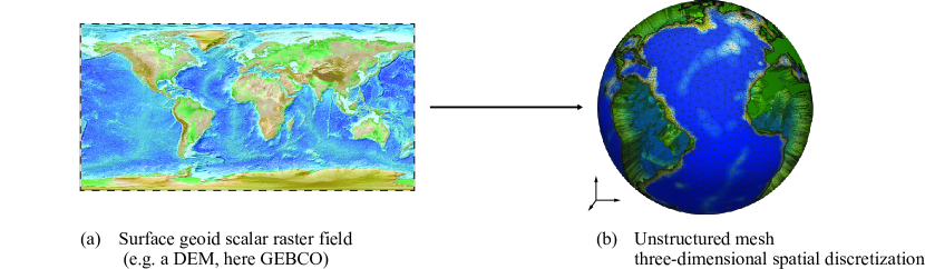
Figure 1: The challenge: to generate a domain discretization that is self-consistent, through a deterministic, automated and repeatable process. Geophysical model spatial discretizations are typically the product of multiple data sources and types (see figure 2). Fundamental to the approach here is the systematic development from a self-consistent data source, such as a surface geoid scalar raster field (a), e.g. the GEBCO (2014) DEM, to an unstructured mesh 3D spatial discretization (b).

Unstructured mesh approaches have the potential for distinct advantages over regular, structured grids. Flexible conforming boundaries can accurately follow the complex, fractal-like bounds typically found in geophysical domains, such as ocean coastlines and bottom bathymetry. With local features exhibiting strong control over ocean dynamics (Danilov et al., 2013), this can provide a more faithful, conforming representation. Unstructured methods additionally support a flexible, variable spatial resolution. With ocean processes evolving over a diverse range of spatial and temporal scales (e.g. see Kantha and Clayson, 2000, p55) – from the large scale thermohaline circulation, significant latitudinal variation in Rossby effects, tides, down to internal and gravity waves, double diffusion and oceanic turbulence – resolved spatial resolution can be optimized (e.g. Sein et al., 2016) and efficiently capture a larger range of spatial inhomogeneities to avoid nesting, using instead a seamless transition between large and small scales, reducing also reliance on empirical parameterizations. Moreover, unstructured approaches have the potential to be more computationally efficient as finer scales are included, with Holt et al. (2017) estimating a factor of 5–17 times less resources required. Whilst unstructured mesh models may not replace structured modeling approaches completely, Danilov et al. (2013) highlight there are certainly cases where this type of approach could be optimal.

The development of unstructured methods for ocean modeling have been actively discussed for the past fifteen years at the annual IMUM (2016) workshops (Ham et al., 2009, Ocean Modelling special issue), with a focus on addressing problems in dynamical core discretizations. Not only are the numerical discretizations of unstructured models more complex, but there exist challenging hurdles in their setup and initialization, notably mesh generation. Relative to regular gridded models, which fundamentally require only a simple land mask to define domain bounds with data remaining in a structured array format, now a heterogeneous range of data types are required and more advanced processing demanded. This is an additional significant barrier to wider adoption, outside the specialist community.

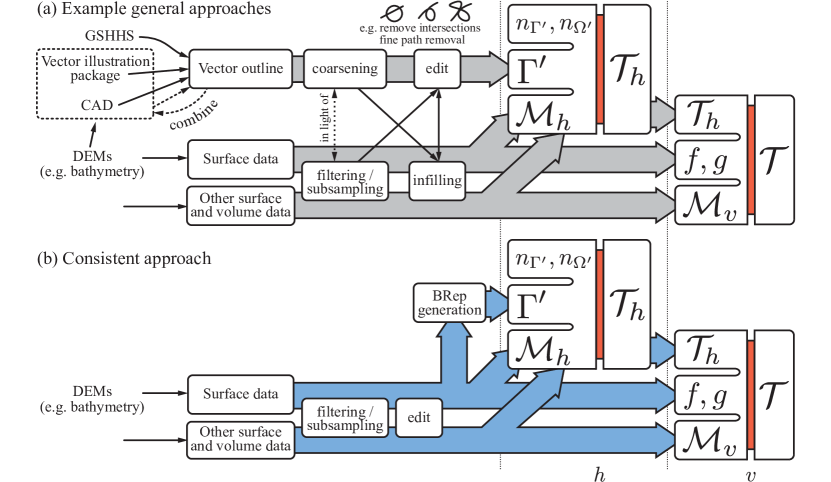
Figure 2: Approaches to unstructured mesh generation for geophysical models, highlighting (a) the case in general and (b) the consistent approach introduced here, with data pathways colored in grey and blue, respectively. The connecting red sections represent spatial discretization processes $h$ 7 and $v$ 8, that are fully constrained by the heterogeneous set of parameters provided to the left, and result in the output discretization to the right. The former $h$ provided by an established Delaunay triangulation implementation for example, to generate the 2D tessellation $\mathcal{T}_{h}$. With $v$, for 3D discretisations, an advancing front algorithm to extrude this tessellation $\mathcal{T}_{h}$ out to $\mathcal{T}$.

Existing methods (reviewed in Candy et al., 2014) to construct underlying spatial discretizations (which, for the purposes of the discussion here, specifically refers to the division of a continuous spatial domain into discrete parts – a discrete tessellation or honeycomb – a generalized notion of triangulation) tend to be model or application specific, labor intensive and difficult to reproduce, or for a single purpose of testing to advance numerical discretization development. These leave mesh discretizations difficult to edit and adjust, when this flexibility is exactly one of the key advantages to unstructured mesh approaches. Processes are often not well documented or accessible to those new to the field. There is the demand for a generic method, accessible to a wide range of modelers, formalizing spatial discretization description for interaction with intercomparisons, to support and take full advantage of the now growing class of mature unstructured mesh numerical simulation models in the field.

The challenge is summarized in figure 1: to generate an unstructured spatial discretization through a deterministic and automated process from a set of self-consistent geoid surface geospatial data fields, ensuring the self-consistency of data is propagated to the resulting spatial discretization (see figure 2). Domain bounds are becoming increasingly complex as simulations include a wider range of scales, with Holt et al. (2017) predicting global models will include coastal scales down to 1.5km in the next 10 years. With the range of scales, physics and required datasets diversifying, it is a new and increasingly difficult challenge to ensure meshes and components in their construction are mutually consistent.

The objective of this paper is to provide:

1. A concise, formal description of the constraint problem (section 2.4, specifically constraints 2).

2. The solution requirements (section 2.5, specifically table 1).

3. Introduce a consistent approach to the generation of boundary representation to arbitrary geoid bounds (sections 4, 5 and 6).

4. Enabling rigorous unstructured mesh generation in general, for a wide range of geophysical applications, in a process that is automated, quick-to-draft and repeat, rigorous and robust, and consistent to the source data throughout (figure 2).

This is implemented in the library developed as part of the project Shingle (2011–2017), and actively being applied in a range of current modeling studies, the details of some of which are discussed in section 7.

The paper is structured such that the following section 2 sets out a formal description of the problem in generating a discretization of geophysical domains and the challenge. The new approach starts in section 3 with self-consistent preparation of source datasets, followed by accurate boundary representation (BR), spatial resolution and identification, in sections 4, 5 and 6 respectively. Generality of the approach is shown by the range of example applications, including verification cases, presented in section 7, followed by conclusions.

2 A complete description of domain discretization for computational geophysical models

2.1 Domain description

Computational representations and manipulation tools of 3D objects have traditionally been built up using a Constructive Solid Geometry (CSG) approach in Computer Aided Design (CAD), where Boolean operations are applied to primitive objects to develop the shape of the full domain, $\Omega\!\subset\!\mathbb{R}^{3}$. These CAD based tools have been extended to enable mesh generation within the bounds of CSG defined objects (e.g. COMSOL, 2016; GiD, ; CUBIT Development Team and Jankovich, 2014). These approaches have been further extended to geophysical applications with for example, GEOCUBIT (Casarotti et al., 2008) and boolean operations on primitive objects to carve out an ice sheet in Humbert et al. (2009) using COMSOL. Whilst these processes can be robust, and possible to automate to make less labor intensive, it soon becomes a significant computational burden for domain surfaces containing complex, multi-scale boundaries which require an increasing number of 3D object intersection calculations. Alternatively, a domain $\Omega$ is described in terms of its bounding surface $\Gamma$. Just like the use of B-rep descriptions provide more flexibility in defining the curved surfaces of CSG objects, this approach offers the possibility to develop efficient descriptions that accurately follow complex geophysical boundaries.

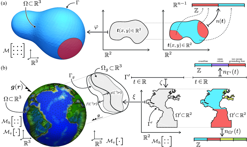
Figure 3: Breakout schematic of mesh generation for (a) general unstructured spatial discretization and (b) typical geophysical domains, referencing constraints 1 and 2 of section 2.4.

2.2 Constraints required to fully describe general domain discretizations

The spatial domain discretization, or generation of meshes, for computational simulation in a domain $\Omega\subset\mathbb{R}^{n}$, illustrated in the schematic (a) of figure 3, requires constraining the following:

Constraints 1

(General spatial domain discretization): The spatial domain discretization for computational simulation in a domain $\Omega\subset\mathbb{R}^{n}$, requires constraining a

• Boundary representation of the bounding surface $\Gamma\subset\mathbb{R}^{n-1}$, an $n\!-\!1$ dimensional manifold, defined using a parameterization $\boldsymbol{t}$ under the homeomorphism

  $$\hskip 6.00006pt\Gamma\!:\boldsymbol{t}\in\mathbb{R}^{n-1}\mapsto\varphi(\boldsymbol{t})\in\mathbb{R}^{n},$$

  including geometric constraints and the boundary identification

  $$\hskip 6.00006ptn\!:\boldsymbol{t}\in\mathbb{R}^{n-1}\mapsto n(\boldsymbol{t})\in\mathbb{Z},\textrm{ and an}$$

• Element edge-length resolution metric, described by the functional

  $$\hskip 6.00006pt\mathcal{M}\!:\boldsymbol{x}\in\Omega\mapsto\mathcal{M}(\boldsymbol{x})\in\mathbb{R}^{n}\!\times\!\mathbb{R}^{n}.$$

2.3 Spatial decoupling of the geophysical system

Gravitational acceleration plays a dominant role in the evolution of geophysical systems, with dynamics decoupled in locally orthogonal directions. Buoyancy-driven effects force processes in the local 1D vertical direction aligned with gravity, distinct from those constrained to the 2D geoid plane ($\Omega_{g}$ in figure 3).

This decoupling and significant difference in spatial and temporal evolution scales between the two motivate numerical simulation models to treat these orthogonal directions differently. Significant process has been made in unstructured ocean modeling based on depth-integrated equations e.g. ADCIRC, FVCOM, H2Ocean, SLIM, T-UGOm) which calculate flow variation on the geoid plane. Extensions to these calculate corrections to include non-hydrostatic effects in the orthogonal local direction (like the mode splitting employed by the MITgcm, Marshall et al., 1997), and in some cases solve in three-dimensions directly (e.g. Fluidity), again with special consideration of the directional decoupling to maintain hydrostatic (Ford et al., 2004) and geostrophic (Maddison et al., 2011) balances, apply geometrically based multigrid (Kramer et al., 2010) and specifically treat the acute aspect ratios found in geophysical domains (Candy, 2017).

This decoupling motivates a development of spatial discretization in parts, in order to best support the associated dynamics, considering first the geoid plane, and secondly, if needed, an extrusion extending this in the normal direction. The significant challenge in this problem is the spatial discretization of the geoid plane, which is common to all unstructured numerical modeling approaches, whether their dynamical cores require two- or three-dimensional discretized domains. As a result, this consideration and resulting approach is applicable to all unstructured models of phenomena dominated by geophysical processes.

2.4 Constraints required to fully describe geophysical model domain discretizations

In this case the constraints are increased, with those of constraints 1 above being further divided, such that mesh characteristics on the geoid plane are considered independently of those in the perpendicular direction of gravitational acceleration. For domains in $\mathbb{R}^{3}$, these become the following:

Constraints 2

(Geophysical spatial domain discretization): The spatial domain discretization for a computational geophysics simulation in a domain $\Omega\subset\mathbb{R}^{3}$, requires constraining a

• Geoid boundary representation $\Gamma_{g}$, of the geoid surface $\Omega_{g}\subset\mathbb{R}^{3}$ that results from the inverse prolongation operation of the required domain $\Omega\subset\mathbb{R}^{3}$ along the gravitational vector. This is the maximal extent of the domain in the geoid plane. Under a homeomorphism $\xi$, this is considered as the chart $\Omega^{\prime}\subset\mathbb{R}^{2}$, such that the boundary $\Gamma^{\prime}$ is described by

  $$\hskip 6.00006pt\Gamma^{\prime}\!:t\in\mathbb{R}\mapsto\zeta(t)\in\mathbb{R}^{2},$$ (1)

  an orientated vector path of the encompassing surface geoid bound defined in 2D parameter space, with a

• Geoid resolution metric for dynamics aligned locally to a geoid, described by the functional

  $$\hskip 6.00006pt\mathcal{M}_{h}\!:\boldsymbol{x}\in\Omega^{\prime}\mapsto\mathcal{M}_{h}(\boldsymbol{x})\!\in\mathbb{R}^{2}\!\times\!\mathbb{R}^{2}\!,\textrm{ together with}\!\!\!\!$$ (2)

• Boundary and region identification, prescribed by

  $$\hskip 6.00006ptn_{\Gamma^{\prime}}\!:t\in\mathbb{R}\mapsto n_{\Gamma^{\prime}}(t)\in\mathbb{Z},\textrm{ and}$$ (3)

  $$\hskip 6.00006ptn_{\Omega^{\prime}}\!:\boldsymbol{x}\in\Omega^{\prime}\mapsto n_{\Omega^{\prime}}(\boldsymbol{x})\in\mathbb{Z},\textrm{ respectively,}$$ (4)

gives the geoid ‘horizontal’ domain discretization (a tessellation) of $\Omega^{\prime}\subset\mathbb{R}^{2}$, with identification elements, all denoted by $\mathcal{T}_{h}$. This together with

• Surface bounds, height maps defined on the surface geoid domain, described by the functions

  $$\hskip 6.00006ptf,g\!:\boldsymbol{x}\mapsto\mathbb{R}\quad\forall\boldsymbol{x}\in\Omega^{\prime},\textrm{ and a}$$ (5)

• Vertical resolution metric for dynamics in the direction of gravitational acceleration (e.g. buoyancy driven), described by the functional

  $$\hskip 6.00006pt\mathcal{M}_{v}\!:\boldsymbol{x}\in\Omega\mapsto\mathcal{M}_{v}(\boldsymbol{x})\in\mathbb{R},$$ (6)

gives the full domain discretization (of $\Omega\subset\mathbb{R}^{3}$) with identification elements, all denoted by $\mathcal{T}$.

This further restriction of constraints is illustrated in figure 3(b), and we note that spatial discretization descriptions satisfying constraints 2 satisfy the more general constraints 1. See Kramer et al. (2010) for further details of the inverse prolongation operation referred to above.

In summary, the horizontal discretization $\mathcal{T}_{h}$ is constrained by: the surface geoid domain $\Omega_{g}$ which is efficiently described in 2D space as $\Omega^{\prime}$, constrained by a BR line $\Gamma^{\prime}$ (1) parameterized under $t$; the geoid element edge-length metric $\mathcal{M}_{h}$ (2); together with boundary and region identifications, $n_{\Gamma^{\prime}}$ (3) and $n_{\Omega^{\prime}}$ (4) respectively, such that,

$$h\!:\{\Gamma^{\prime},\mathcal{M}_{h},n_{\Gamma^{\prime}},n_{\Omega^{\prime}}\}\mapsto\mathcal{T}_{h}.$$ (7)

The full discretization $\mathcal{T}$ of the 3D domain $\Omega\subset\mathbb{R}^{3}$, is then constrained by: this geoid discretization $\mathcal{T}_{h}$; surface bounds $f(\boldsymbol{x})$ and $g(\boldsymbol{x})$ (5) defined on $\boldsymbol{x}\in\Omega^{\prime}\subset\mathbb{R}^{2}$, that provide height extrusions in directions parallel to local $\boldsymbol{g}(\boldsymbol{r})$ for $\boldsymbol{r}\in\mathbb{R}^{3}$; together with a vertical edge-length metric $\mathcal{M}_{v}$ (6), such that,

$$v\!:\{\mathcal{T}_{h},f,g,\mathcal{M}_{v}\}\mapsto\mathcal{T}.$$ (8)

A consequence of this development is that whilst spatial discretizations are unstructured in all three local coordinate directions, they are constrained to ensure cell faces lie parallel or perpendicular to geopotential surfaces and dominant flow features, such that fluxes can be calculated accurately and errors in the calculation of pressure minimized (Danilov et al., 2008; Kramer et al., 2010). This development is illustrated in the right hand side of the schematic in figure 2, common to both (a) and (b).

2.5 Challenges in domain discretization for geophysical models

Mesh generation for regular-gridded models is simply a matter of identifying which elements lie in the simulation domain through mask fields and all data involved in the process is in the same 2D spatially-indexed scalar raster form, using now standard operations for data on structured grid ocean models (Cotter and Gorman, 2008). For unstructured spatial discretizations, the constraints 2:1, 2, 3, 4, 5 and 6 require a variety of data types, from more standard 2D raster maps, to tensors and vector paths. Notably, the geoid BR (1) is a vector path, in contrast to the 2D scalar data required for the majority of the rest of the constraints 2, 3, 4, 5 and 6, and traditionally the raster forms used in the construction of structured grid meshes. This makes it arguably the most challenging of the constraints to provide, ensuring it is an accurate and faithful representation that is consistent with 2, 3, 4, 5 and 6. Under this now heterogeneous set of constraints, both the mesh description and generation problem are significantly more complex than the structured case (summarized as the nine tenets of geophysical mesh generation in table 1).

1. Accurate description and representation of arbitrary and complex boundaries such that they are contour-following to a degree prescribed by the metric size field, with aligned faces so forcing data is consistently applied ($\Gamma^{\prime}$, $f$, $g$).

2. Spatial mesh resolution to minimize error; with efficient aggregation of contributing factors, ease of prototyping and experimentation of metric functions and contributing fields, complete over the entire extent of the bounded domain ($\mathcal{M}_{h}$, $\mathcal{M}_{v}$).

3. Accurate geometric specification of regions and boundary features; to provide for appropriate interfacing of regions of differing physics, model coupling and parameterization application ($n_{\Omega^{\prime}}$, $n_{\Gamma^{\prime}}$).

4. Self-consistent, such that all contributing source data undergoes the same pre-processing, ensuring self-consistency is inherited.

5. Efficient drafting and prototyping tools,

   such that user time can be focused on high-level development of the physics and initialization of the modeled system.

6. Scalability, with operation on both small and large datasets, facilitating the easy manipulation and process integration, independent of data size.

7. Hierarchy of automation, such that individual automated elements of the workflow can be brought down to a lower-level for finer-scale adjustments.

8. Provenance to ensure the full workflow from initialization to simulation and verification diagnostics are reproducible.

9. Standardization of interaction to enable interoperability between both tools and scientists.

Table 1: The nine tenets of geophysical mesh generation, that solutions to the spatial discretization of geophysical model domains should address.

Vector path descriptions are significantly more complex to store, interrogate and develop. Control points of higher-order representations such as polynomial splines or flexible non-uniform rational B-splines (NURBS) do not necessarily lie on the bounding path. Operations cropping to subregions, subsampling and merging are no longer simple selection, local binning routines, or efficient filtering matrix multiplications. The path description should be an orientated vector generated to a required, spatially variable, level of accuracy (item 1) in a rigorous and reproducible (item 8) manner. In addition to ensuring paths accurately represent key geographic features (item 1) and are efficiently stored (optimized following algorithms such as Douglas and Peucker (1973), for example) it is important vector paths are topologically correct. Line descriptions need to be closed to define fully bounded regions, that are disjoint and correctly orientated to identify which side of the path is to be included in the domain described.

Existing datasets of orientated vector paths

To avoid issues in constructing these vector paths, modelers can use pre-prepared boundary datasets, such as the Global Self-consistent, Hierarchical, High-resolution Geography Database, (GSHHG, previously GSHHS, Wessel and Smith, 1996). Used as distributed, this data can be used successfully in model simulations. The GSHHS plugin (Legrand et al., 2007; Lambrechts et al., 2008) written to interact with Gmsh (Geuzaine and Remacle, 2009) successfully reads the database of pre-prepared coastline contours of GSHHS. Significant progress has been made in unstructured mesh ocean modeling with spatial discretizations generated using Gmsh (e.g. see Legrand et al., 2000; White et al., 2008; van Scheltinga et al., 2010; Gourgue et al., 2013; Thomas et al., 2014). This is a good solution for model problems with domains containing boundaries that can be defined by GSHHS, although inconsistencies can develop when combined with other datasets, to include additional geographic features, or for the bounds 5 for example.

Modifications, in practice, suffer from a lack of sufficient data, and additional external data is required to complete refinements. It is also the case that there are many domains for which a vector boundary path is not available. This has been mitigated to a small degree with the introduction of the updated GSHHG, which additionally includes the CIA World Data Bank II rivers and border database, but again in general this is very limiting. This is the case in ocean domains extending under ice shelves to the grounding line where ice meets bedrock or where it is important to extend over land to include the potential for inundation, in a tsunami model for example, or indeed in modeling geophysics of the past, in paleo-ocean simulations. This is not a solution for arbitrary bounds (item 1) and demands an alternative approach.

Existing methods for boundary representation construction

Terreno (Gorman et al., 2006, 2007) operates directly on DEMs, in line with figure 1, combining BR generation with optimization for shoreline and bathymetry representation. This provides high-quality spatial discretization on a geoid, but is limited in its flexibility and scope to add fine adjustments, and generally in its scope for a hierarchy of automation (item 7).

Vector illustration packages have long been used to handle orientated vector paths and their editing. These have matured over many years of development and contain robust interfaces and efficient manipulation routines. Interfacing with meshing software can be achieved through the standardized Scalable Vector Graphics (SVG) data type, and this is the workflow applied together with Gmsh in Gourgue et al. (2009), de Brye (2011) and Kärnä et al. (2011), and detailed further in Lambrechts and Seny (2011). New BRs for the domains of ancient seas were developed this way in Wells et al. (2010) following Gorman et al. (2008). Illustration tools however, have not been developed for this type of geographic processing, and crucially do not consider projections of the sources or required output. For instance, it is difficult to simplify path descriptions based on spatial distance in this approach.

A solution to this is demonstrated in Candy et al. (2014) using Geographic Information System (GIS) frameworks. These are designed for 2D raster and polyline manipulations and importantly take into account dataset projections and geospatial information. In highly multi-scale applications, this integration with these well-established mapping tools is a good, flexible and more rigorous solution for including intricate boundaries, over a range of scales, such as the man-made structures of a harbor together with the complex, fractal-like coastlines of the UK. With this hand-editing and graphical approach, this is not the whole solution, since it can be difficult to automate (item 7) and reproduce (item 8), and can become limited for complex, multi-scale boundaries, but is an important part of a general geospatially informed solution approach.

3 Self-consistent source data preparation

It is relatively easy to ensure a set of raster fields are mutually consistent (item 4), with geospatially-aware matrix operations simply applied throughout. Matched treatment of corresponding vector paths is a significant challenge. Inconsistencies can develop, with for example BRs lying over regions classified as land in the source bathymetry data, or worse bisecting other parts of the BR.

3.1 Automated generation of a consistent constraint description

Central to the new, generalized approach of figure 2(b) is that the whole discretized domain and forcing fields are built up from a self-consistent input dataset. This dataset may contain multiple fields, but importantly they share a common spatial structure and have undergone the same harmonized processing (item 4). To ensure the process is efficient (item 5), user interaction is focused on generating the consistently processed input dataset and high-level constraint description. With the developed approach, it is then possible to automate subsequent processing to lead to an output mesh and initialization described by the input, an injective deterministic process. This is repeatable and together with a record of the processing required for the input, provides a complete record of provenance (item 8).

3.2 Data preparation and assimilation of datasets

The preparation of data to describe the constraints 2 alone contains many inherent challenges. The BR description (1) should be a continuous, closed, non-intersecting path that is orientated and resolves well important selected geometric constraints (item 1). The spatial resolution size descriptions (2) and (6) need to be complete, defined over the entire geoid surface, appropriately graded so they vary smoothly enough so as not to adversely affect modeled dynamics (Sein et al., 2016; Gorman et al., 2006; Piggott et al., 2005) and minimize numerical discretization error (item 2). Identification (item 3) involves functions mapping over the range of spaces: $\mathbb{Z}$, $\mathbb{R}$ and $\Omega^{\prime}\subset\mathbb{R}^{2}$, typically piecewise constant (e.g. finite element $\textrm{P}_{0}$) representations on the discretized $\mathcal{T}_{h}$ and boundary $\Gamma^{\prime}$ for $n_{\Omega^{\prime}}$ and $n_{\Gamma^{\prime}}$, respectively. The heterogeneous set of constraint parameters and their discrete forms need to be kept mutually consistent in both the description preparation and mesh generation process (item 4), whilst achieving goals expected in scientific model development such as efficient prototyping, scalability, automation, provenance and interoperability (items 5, 6, 7, 8 and 9).

3.3 Resolution appropriate representation

Source data is processed in order to ensure a good representation of fields and domain boundaries in the resulting discretization (see figure 2). A spatially inhomogeneous filtering focuses on areas of interest and provides support for physical phenomena. For consistency, this must be applied equally to all sources, including vector paths, surface bounds and other surface and volume data. This is not a trivial task, particularly in maintaining path consistency with geoid surface spatial datasets, under this variable spatial resolution specification.

3.4 Boundary representation preparation

It is possible to encounter or, under the processing of section 3.3, introduce intersections in path datasets which require removal before BRs are passed on to meshing algorithms (e.g. land boundaries passing through islands or loops in a single path, see figure 2). When hand-edited, a decision is made to separate the island, adjust so they no longer intersect, or simply remove the extra loop. It is also possible that infilling of the spatial datasets is required (Nurser, 2012) to ensure data is available in the region enclosed by these bounding paths. This approach can be time-consuming, prone to human error and lead to inconsistencies.

3.5 Iterative and incremental development

In practice it is often found that a significant proportion of simulation failures for models on unstructured spatial discretizations are due to poor mesh quality (e.g. Griffies et al., 2000), necessitating iterative, incremental changes to the underlying spatial discretization. Additionally, unstructured meshes can contain errors in their construction that can be difficult to identify. It is possible to introduce mesh elements that are free and decoupled from the rest of the domain, or due to the geometry and imposed boundary conditions, are fully prescribed from the outset, containing no independent parameters. This stage often requires significant input from the user; to filter, subsample and hand edit, together with other preparatory stages shown in the context of the full mesh generation pipeline illustrated in figure 2, and strongly motivates an approach which enables quick, efficient prototyping (item 5) and a hierarchy of automation (item 7) for fine adjustments.

4 Consistent generation of boundary representation constraint description

4.1 Boundary representation constraint data

Constraint of the BR requires an orientated vector path for 1 and for 3D models, 2D scalar height maps complete within the surface geoid for 5. Once the self-consistent source dataset has been prepared, containing all data required to describe constraints 2, the rest of the process in figure 2(b) is automated. The first component is the generation of a suitable geoid BR (1) from this source dataset.

4.2 Bottom-up, highest fidelity representation

At this stage, before requirements on the spatial resolution are considered, it is important the BR is at the fidelity of the given source dataset. This is a bottom-up approach, in the same class as Gorman et al. (2007) and Lambrechts et al. (2008), using the finest definition of the BR polyline, such that it is then coarsened where possible. This is in contrast to top-down approaches to the approximation of domain bounds, such as Douglas and Peucker (1973), which begin with a coarse definition and refine as required. Whilst these can produce better results, they tend to be more expensive to compute.

Beginning with the highest-fidelity representation means adjustment operations are kept local for computational efficiency and can be relatively easily scaled in parallel. It is easier to ensure the resultant discretized boundary is spatially consistent with the metric and vertical bounding fields, starting with a path that is consistent. Geophysical domain geoid surfaces are largely convex, such that more flexible NURBS can be defined on the same control points as piecewise linear path representations whilst maintaining consistency, since the curves remain inside the convex hull of these points. Lastly, with a bottom-up approach, the base description contains all information required to generate a full hierarchy of complexity in model domains, such that it fully parameterizes $\Gamma^{\prime}$, required for constraint (1) and the functional $h$ 7, and thus can be shared for full reproducibility.

4.3 Identifying the geoid boundary representation

The self-consistent fields are combined to form a mask identifying geoid bounds of the domain in directions parallel to geoid surfaces, described by the functional

$$\boldsymbol{x}\in\Omega^{\prime}\mapsto\mathcal{F^{\prime}}(\boldsymbol{x},S_{0}(\boldsymbol{x}),S_{1}(\boldsymbol{x}),\ldots)=\mathcal{F}(\boldsymbol{x})\in\mathbb{R},$$ (9)

for source data $\boldsymbol{x}\in\Omega^{\prime}\mapsto S_{i}(\boldsymbol{x})$, functions from $\mathbb{R}^{2}$ evaluating to variables of arbitrary rank and data type, that are suitably reduced by the functional $\mathcal{F}$ to a scalar field. It is the contour of this mask that defines the geoid BR $\Gamma^{\prime}$, such that

$$\Gamma^{\prime}\!:\;\;[t_{0},t_{1}]\subset\mathbb{R}\mapsto\zeta(t)\in\mathbb{R}^{2},\ \textrm{where}\;\;\mathcal{F}(\zeta(t))=c,$$ (10)

for a constant $c$. In the case of a normalized mask centered about the boundary, where $\mathcal{F}\in[-1,1]$, a constant value of $c=0.0$ is taken. For more common operations, a selection of forms for the functional $\mathcal{F}$ are available in the Shingle library, with arbitrary functionals possible written directly as Python expressions.

The well-established and robust Generic Mapping Tools suite (GMT, ) contains methods to generate contours from 2D raster fields, and could be used to solve (10). It was found however, that the output GMT paths did not contain enough information to form a well-defined BRs on the geoid surface with distinct closed and open contours. The process was also dependent on writing and reading multiple plain text files, which soon became inefficient as larger problems were considered.

We solve (10) in the 2D parametric space of $\Omega^{\prime}\in\mathbb{R}^{2}$, under a homeomorphic projection $\xi$ that preserves neighbors (see section 5.2), in an approach built up from standard Python libraries. In practice, in the scenarios presented in section 7, this is a cylindrical Mercator, stereographic or, over relatively small geoid patches, the Universal Transverse Mercator (UTM, see Snyder, 1987) projection. Since there is no restriction this be isometric or area-preserving, and moreover the preparatory stage may have intentionally yielded data at varying resolutions, points in $\Omega^{\prime}$ are not necessarily equally spaced or representative of target discretized resolution. Spatial measures are calculated on $\Omega$, made under the transform to 3D Euclidean space and take into account curvature of the geoid surface.

Unlike existing approaches using GSHHS vector paths or attempting to use paths generated by GMT, we have access to more information at this stage. Alongside a description of polylines, there is additionally access to path orientation, implied boundary IDs, region IDs, whether paths require closing, physical boundaries, and imposed simulation boundaries, e.g. for simulation forcing. The result is that the generation of the components required for $\mathcal{T}_{h}$ can be achieved consistently and largely automated, to minimize user edits and maintain a robust approach.

4.4 Boundary closure

The constraint (1) and associated resultant surface may: (i) have a non-zero genus and contain island holes within the domain, (ii) yield more than one closed contour path, (iii) contain open convex and concave paths. It is important these are handled automatically to ensure items 5, 6 and 7 are met.

For a simply connected surface with a zero genus and no island holes, $\zeta(t_{0})=\zeta(t_{1})$ ensures the BR is closed. This is easily extended to non-simply connected surfaces with a non-zero genus with multiple intervals $[t_{0},t_{1}]\subset\mathbb{R}$, with a reversed vector path orientation denoting regions excluded from the surface.

At this stage open boundaries require closing to complete the domain such that it is consistent to metrics and surface bounds defined on the geoid, and identified correctly. Boundaries are often closed along meridians and parallels, such that the domain is easy to specify and to facilitate model intercomparisons, where, for example, forcings are provided on these closures. This is relatively easy to achieve in structured models, where element faces typically lie on orthodromes, and often motivates their choice as bounds. The approach depends on projections to different topological spaces for operations throughout the process (through interaction with the established and robust PROJ.4 ). Open boundary path closures are drawn under UTM, based on reference points local to the region, which are distance preserving and ensure minimal distortion.

4.5 Path verification

With the bottom-up approach taken, the finest resolution of the BR is inherited from the source dataset, which itself has been prepared to be at the minimum goal fidelity, it is also possible to now check properties of the paths to eliminate features which could introduce problems at simulation time, e.g. an evaluation of path curvature, or a coarse check of the angle between successive segments. Preliminary diagnostics on the BR at this point provides direction for further processing of the source input dataset, and an iteration of this process to improve boundary selection and ultimately develop the best consistently generated mesh (pursued further in Candy and Pietrzak, 2017).

With access to the highest resolution path data and associated projection information at this stage makes it possible to further automate additional processing, which is not possible or difficult with other approaches, such as the explicit removable of islands by land area, or the automatic identification of inflows from river runoff. In large multi-scale simulations there can be thousands of such features which makes processing time-consuming, error prone and severely impacts automation and the efficient drafting and prototyping. This is particularly important if the process illustrated in figure 2(b) is to be repeated and iterated on.

5 Consistent generation of spatial resolution constraint description

5.1 Spatial resolution constraint data

Spatial resolution is defined in two orthogonal components following the decoupling of section 2.3. This requires a functional 2D dyad, a rank 2 tensor field defined complete over the surface geoid $\Omega^{\prime}$ for $\mathcal{M}_{h}$ (2) and for 3D models, a scalar field defined complete over the whole domain $\Omega$ for $\mathcal{M}_{v}$ (6). The latter efficiently defined in a domain bounded by $\Omega^{\prime}$, $f$ and $g$ (defined on $\xi^{-1}(\Omega)$, see figure 3), which determines the vertical coordinate system (see section 6.4).

5.2 Chart homeomorphism choice

Location on the surface geoid $\Omega_{g}\subset\mathbb{R}^{3}$ is defined by two orthogonal linearly independent variables. For efficiency of calculations and storage constraints 1, 5, 2, 3, 4, 5 and 6 are defined on $\Omega^{\prime}\subset\mathbb{R}^{2}$ under the homeomorphism $\xi$, which maps to 3D space, and together form the chart $(\xi,\Omega^{\prime})$, such that

$$\xi\!:\boldsymbol{t}\in\Omega^{\prime}\mapsto\xi(\boldsymbol{t})\in\Omega_{g}\subset\mathbb{R}^{3},$$ (11)

where there exists a unique point $\boldsymbol{t}$ in $\Omega^{\prime}$ for every point $\xi(\boldsymbol{t})$ on the surface geoid in the simulation domain $\Omega_{g}$, i.e. a bijective, invertible mapping so it is possible to move back and forth between chart and real 3D Euclidean space. Additionally the mapping should be continuous, to preserve continuity of the surface geoid.

Where $\Omega^{\prime}$ is also the domain required by the simulation model (e.g. local UTM or longitude-latitude cylindrical Mercator, such as ADCIRC) post-processing of the output mesh is simplified, although care is required to ensure $\xi$ in (11) matches exactly that used within the model itself. Where simulation calculations proceed in 3D Euclidean space $\xi$ is required as a post-processing step to map output to Cartesian coordinates in $\mathbb{R}^{3}$. For simulation domains lying in a space distinct from $\Omega$ and $\Omega^{\prime}$ (e.g. spherical polar coordinates) a further homeomorphic projection is required. This does not affect the consistency of the approach, but permits a flexible choice of chart specific to domain discretization and model simulation calculations.

In addition to working in a 2D chart, it is beneficial to choose a homeomorphism $\xi$ that is conformal to minimize extremes in element anisotropy in the space $\Omega^{\prime}$ over which the 2D meshing algorithms operate. For a global shell, a convenient conformal homeomorphism is the stereographic projection with the point antipodal to the center of projection removed (see Snyder, 1987; Lambrechts et al., 2008; Gorman et al., 2006). The following form of stereographic projection is applied in combination with a standard spherical coordinate mapping to establish $\xi$ in the section 7 applications to global oceans, ice shelf ocean cavities and Southern Ocean (SO)

$$\xi\!:(x,y)\in\mathbb{R}^{2}\mapsto(x,y,z)\in\mathbb{R}^{3}\!,\ \textrm{with}\ \xi=\beta\alpha^{-1}\!,\,\textrm{where}$$

$$\qquad\alpha(\psi,\phi,r)=2r\,\mathrm{tan}\left(\frac{\pi}{4}-\frac{\phi}{2}\right)(\mathrm{sin}\ \psi,-\mathrm{cos}\ \psi),$$

$$\qquad\beta(\psi,\phi,r)=r(\mathrm{sin}\,\phi\ \mathrm{cos}\,\psi,\,\mathrm{sin}\,\phi\ \mathrm{sin}\,\psi,\,\mathrm{cos}\,\phi).$$ (12)

To be bijective, the surface cannot include the projection point, which is propagated to infinity in the stereographic plane. In the case of global ocean models this is achieved by slicing part of the land away at the South Pole to produce a truncated spherical shell that is homeomorphic to a single-point compactification of a 2D plane. For smaller regional models on the sphere, this modification choice is more easily made.

Projections including multiple charts or mappings that are not strictly homeomorphic can be handled with special treatment. In the case of cylindrical Mercator, the format typically used for global Earth datasets, with $\Omega^{\prime}$ cast in longitude-latitude space, the topological atlas includes a homeomorphism that although conformal, is not bijective and continuous along a meridian and at the poles. Shingle automatically stitches together BR vector paths broken across this edge meridian seam, a fixing procedure made for GSHHS paths in Lambrechts et al. (2008). In the subsequent spatial discretization to this BR description, this issue is avoided using an azimuthal projection, such as stereographic (12).

With the surface geoid BR $\Gamma^{\prime}$, element metric $\mathcal{M}_{h}$, and identifications $n_{\Gamma^{\prime}}$ and $n_{\Omega^{\prime}}$ generated following the consistent approach outlined above to form the heterogeneous self-consistent constraint set $\{\Gamma^{\prime},\mathcal{M}_{h},n_{\Gamma^{\prime}},n_{\Omega^{\prime}}\}$, corresponding to the constraints 2:1, 2, 3 and 4 respectively, the discretization $\mathcal{T}_{h}$ can be generated following the process $h$ (see 7 and 2). Shingle forms an accurate description of these first four constraints into a syntax that can be interpreted by the meshing library which in turn solves the spatial discretization problem under these constraints.

5.3 Interpretation and processing of the high fidelity constraint descriptions

In the examples presented in section 7, Shingle prepares the constraint set in a syntax that can be interpreted by the meshing library Gmsh (Geuzaine and Remacle, 2009) for discretization of the geoid domain $\Omega^{\prime}$ in the process $h$ 7. Gmsh is chosen because, through its standard syntax, it opens up access to a range of generic meshing algorithms that have been demonstrated robust with other approaches (section 2.5). It is equally possible to develop communication interfaces with other meshing packages and libraries, some of which can interact directly in Python (e.g. the Triangle Library Python Bindings (2014) to the Triangle library, Shewchuk (2002)), discussed further in Candy and Pietrzak (2017). For a full 3D discretization, the remaining constraints (5) and (6) are stored efficiently as fields on binary unstructured VTK data structures containing a description of the spatial geoid discretization $\mathcal{T}_{h}$. The first stage is a reparameterization of the geoid BR (10) produced by Shingle, to take into account the mesh size field $\delta(\boldsymbol{x})$ derived from $\mathcal{M}_{h}$, according to

$$\int_{t_{0}}^{\tilde{t}_{i}}\frac{1}{\delta(\boldsymbol{x})}\left\|\frac{\partial\xi(t)}{\partial t}\right\|\,\mathrm{dt}=i,\quad\textrm{for}\ i\in[0,1,\ldots,n],$$ (13)

for the $n+1$ new points along the boundary at parametric coordinates $\tilde{t}_{i}\in\{\tilde{t}_{0},\ldots,\tilde{t}_{n}\}$, with $\left\|\partial\xi(t)/\partial t\right\|$ the length-scale Jacobian of the homeomorphic parametric mapping $\xi$ .

The approach developed here and implemented within Shingle ensures solution high-fidelity BRs calculated from (10) are inherently non-intersecting. The meshing algorithms within the Gmsh library do not natively maintain this (with use of the adaptive trapeze rule for integrations to solve (13)) but this has been addressed with the systematic recovery procedure described in Lambrechts et al. (2008). It is again important this is an automated algorithm, since it cannot be handled rigorously and efficiently by hand when there is potential for multiple cases in the complex bounds of geophysical domains. This provides an initial 1D computational mesh of the domain boundary $\Gamma^{\prime}$ on the geoid.

The full computational meshing of the geoid surface $\Omega^{\prime}$, given the discretization of the boundary and geoid element metric $\mathcal{M}_{h}$, is achieved by Gmsh through first an initial seeded Delaunay triangulation constrained to include the 1D boundary mesh. This is then optimally restructured using standard and robust approaches available in meshing libraries, here: an anisotropic Delaunay method (George and Borouchaki, 1998), a frontal algorithm (Rebay, 1993) or a local modification technique (see Geuzaine and Remacle, 2009; Lambrechts et al., 2008). The latter is similar to the method of mesh generation described in Gorman et al. (2006), and the routines applied to adapt the mesh in time in response to solution dynamics, as described in Pain et al. (2005). There is no need to reimplement these methods, and instead we build on them and interact through standardized APIs and data structures.

5.4 Boundary representation genus adjustment

The geoid surface $\Omega^{\prime}$ can be non-simply connected with a non-zero genus (section 4.4). For scales in the horizontal metric $\mathcal{M}_{h}$ larger than these breaks in the surface, the discretized boundary is coarsened from the high fidelity BR following (13), but it is better to eliminate the BR contribution entirely, and parametrize its influence. In practice, meshing algorithms struggle to perform this elimination. Shingle removes these features during the preparation of (1) by comparing their geoid extent to the metric $\mathcal{M}_{h}$ in its locality, or simply by a minimum area criteria. Lengths and areas are calculated and compared in a projection that is local and appropriate to the intended simulation, giving an accurate measure of distance on the geoid surface.

An alternative approach, also performed through Shingle in the examples of section 7, is to filter out these features through the filtering / subsampling stage shown in figure 2(b), and to a spatial resolution from $\mathcal{M}_{h}$. This leads to a more consistent set of constraints {$\Gamma^{\prime}$, $f$, $g$, $\mathcal{M}_{h}$, $\mathcal{M}_{v}$, $n_{\Gamma^{\prime}}$, $n_{\Omega^{\prime}}$} and is also how to handle groups of features, which can be agglomerated together at this filtering / subsampling stage to generate a larger-scale BR and consistent 2D fields of the group together.

5.5 Constraints over the number of degrees of freedom

Spatial resolution is limited by the overall number of degrees of freedom and available computational resources, directly through available memory and indirectly by the cost of inter-node communications. The maximum number of degrees of freedom can be a more natural constraint, rather than the element edge-length metrics of $\mathcal{M}_{h}$ and $\mathcal{M}_{v}$. Unstructured mesh models permit a multi-scale heterogeneity in spatial scales within a single discretization and subsequent simulation. This makes constraining on a maximum number of degrees of freedom no longer a simple arithmetic operation from a global spacing size. Once the spatial pattern of element edge-lengths has been constructed as a functional of scalar fields, together with information of the order of representation made for prognostic simulation fields that need to be stored in memory and potentially shared between nodes, there is enough information to constrain on the maximum number of degrees of freedom. The inverse of the functionals determining $\mathcal{M}_{h}$ and $\mathcal{M}_{v}$ are used to calculate an approximate number of spatial nodes and degrees of freedom in an output discretization, which in turn is used as a constraint on these metrics. This simply scales the element edge-lengths globally, or interacts in the functional to adjust the spatial pattern, limiting the smallest element edge-length for example, whilst the largest spatial spacing is maintained constant.

5.6 Anisotropic spatial constraint

The approach makes no restrictions over mesh element aspect ratios, which are free to be fully anisotropic. Anisotropy is strongly motivated in the orthogonal decoupled local horizontal and vertical directions by the differing physics characterizing geophysical systems highlighted in section 2.3. This is easily developed within the constraints 2 that describes and subsequently handles spatial discretization in these distinct directions in separate processes. Within the geoid surface, anisotropy in the local plane orthogonal directions is prescribed by the tensor field $M_{h}$ of 2.

6 Identification of bounds and regions

Identification of regions on and within the surface boundary is required in order to apply geometric constraints and boundary conditions during a simulation, providing (3) and (4) of constraints 2. The former identifies edges of the domain $\Omega$ with normals orthogonal to local gravitational acceleration. The remaining surfaces, that lie on the extruded geoid bounds defined by the scalar functions $f$ and $g$, are identified by the latter. This second identification function also partitions the volume, for the application of simulation-time body forcings, viscosity parametrizations, vertical turbulence parametrizations and vertical coordinate systems, for example.

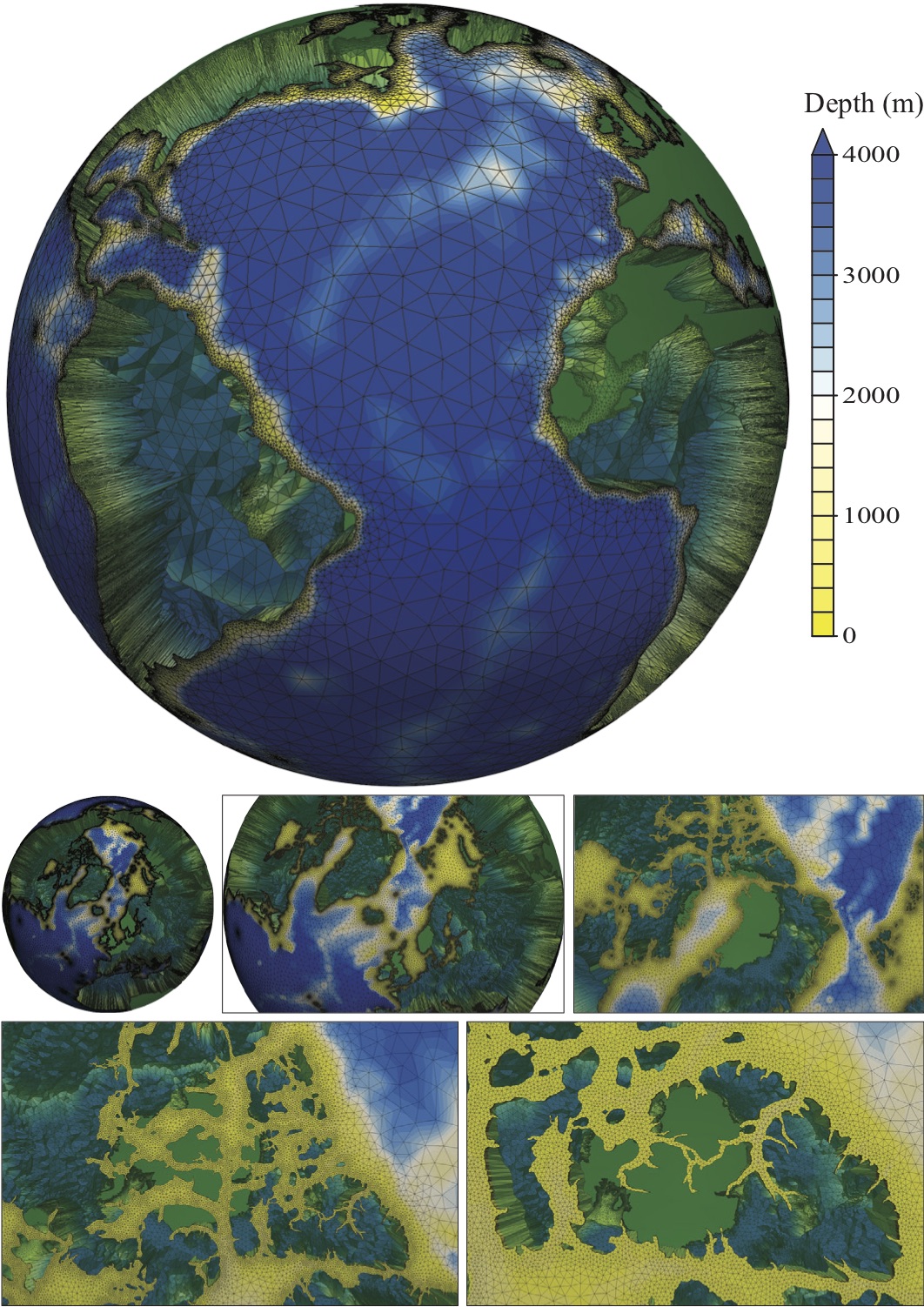
Figure 4: Full mesh $\mathcal{T}$ of the global oceans containing a multi-scale of spatial resolutions, parallel to the geoid, from $10\textrm{km}$ to $500\textrm{km}$, and vertical layers spaced from $2\textrm{m}$ to $500\textrm{m}$, under differing regimes from $\sigma-$layers in ice-covered and coastal regions up to the continental shelf, transitioning to $z-$levels in the open ocean. The mesh contains 8,778,728 elements and 35,114,912 spatial degrees of freedom under its discontinuous Galerkin finite element discretization. Zoomed in regions focusing on the complex Canadian Arctic Archipelago west of Greenland around Ellesmere and Baffin island are shown below. The domain has been scaled radially by a factor of 300 in order to show the vertical extent of the discretization of this shell, with land regions shaded green.

6.1 Geometric constraints

Geometric constraints apply physical restrictions on the domain discretization, to ensure, for example, a land run-off outflow source to an ocean model is geographically placed correctly, regions of differing drag are well-represented in an ice sheet or vegetation model, or that the position of a terminating ice front is accurately maintained. Geometric constraints additionally optimize to the numerical discretization, motivated by coupling differing models, nesting or matching to input data. This identification is an integral part of the domain discretization and is best developed and applied while the high fidelity BR is created, since it influences the placement of control points.

6.2 Geoid surface closure

Current approaches which require editing, constraint and identification of the BR by hand are not appropriate for more complex boundaries and an automated method is required. Paths which fall outside the region of interest are truncated, and closed along the edge of the region of interest with joins geometrically constrained, and by default identified differently to the main path internal to the domain so that appropriate boundary conditions can be applied. Geometric constraint of the point of change joins ensure the discretized boundary is represented up to the edge of the region of interest, irrespective of the underlying local edge-element size provided by $\mathcal{M}_{h}$.

6.3 Conforming extensions and closures

For the purpose of model intercomparisons and benchmarks, the domain BR is typically described in terms of geographic contour sections, such as coastlines, bounded by parallels and meridians. The approach automatically extends and closes domains along parallels and meridians, irrespective of projection. The extension of the domain in this way can also be used to naturally include boundary restoring sponge regions in a geometrically consistent manner to ensure these artificially created boundaries are accurate and well-represented, their interpolated positions are calculated in UTM space under a projection relative to a nearby point, and with an appropriate local step size, with positions then mapped back to the required chart.

6.4 Generalized hybrid vertical coordinates

The identification also has direct input to the subsequent discretization stage that develops the extrusion to $f$ and $g$, under $\mathcal{M}_{v}$, and to match with nesting or coupled models. This is used to develop a generalized hybrid vertical coordinate, smoothly varying between $z-$levels and $\sigma-$layers (Haidvogel and Beckmann, 1999; Griffies et al., 2005) in the deep open ocean and coastal regions, respectively. Additionally, a transition hybridized region is defined distinct in $n_{\Omega^{\prime}}$, to limit reflection and rarefaction of waves whose propagation properties are dependent on spatial grid size.

6.5 Demarcation of physical systems

Vertical interfaces internal to the domain $\Omega$ and perpendicular to the geoid, are prescribed by a change in the region identification function $n_{\Omega^{\prime}}$. Alternatively, if the interface is required to be geometrically constrained, this is achieved through a definition of multiple partially adjoining domains $\Omega_{i}$. Both approaches are made in section 7.

The region identification $n_{\Omega^{\prime}}$ additionally tracks the horizontal surfaces over which differing physical simulation models are coupled. An ocean top surface interfaces with both air and ice, and $n_{\Omega^{\prime}}$ is used such that effects from ice–ocean interaction are only applied to a subset of the top ocean surface, e.g. melting and freezing processes, and loading from the ice above. With information on the location of ice draft available in the source dataset (as is the case in RTopo, Timmermann and et al., 2010), the identification can be made under the same treatments that are applied to the bounding surfaces (e.g. bathymetry and ice draft), to keep domain development self-consistent.

7 Application case studies

A range of application examples are presented to emphasize the generality of the flexible and robust approach. This begins with more standard domains such as the global oceans, that can be developed up to a point with other approaches using for example, the coastlines of GSHHG, and proceeds to consider more complex domains bounded on all sides by geometrically intricate surfaces and containing multi-model coupled interfaces, such as ice shelf ocean cavity domains. The basis constraint descriptions of these are available with the library, for use and further development. Some additionally form part of the verification test suite.

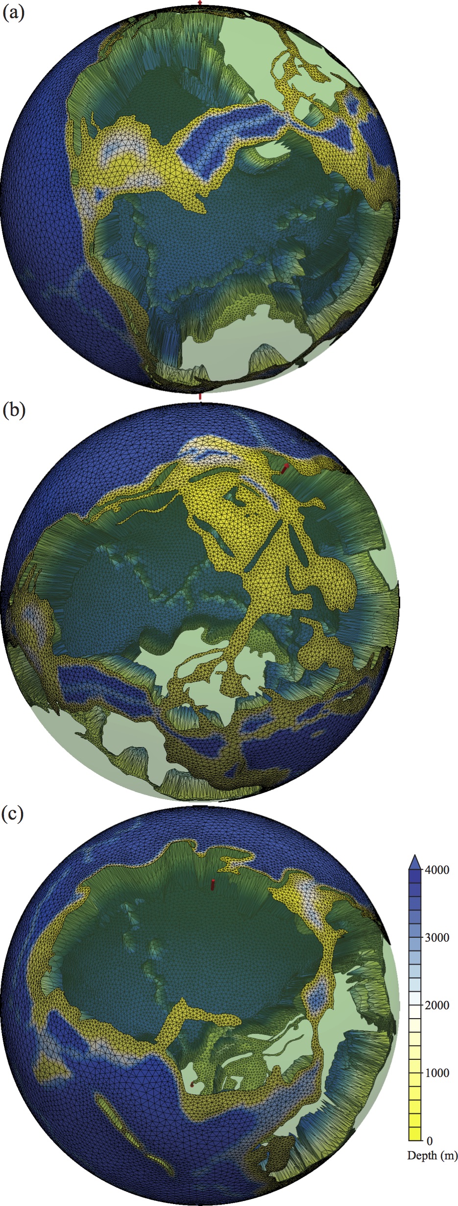
Figure 5: Full discretization of global oceans of the Early Cretaceous Berriasian age $\sim$140 million years ago, enabling research studies of paleo-oceans using variable resolution, boundary-conforming spatial discretizations, that are particularly challenging during this period due to the numerous shallow inland seas present from high eustatic sea levels. The shell domain is radially stretched as per figure 4. (a) Mid-Atlantic ridge central with North America above, West Gondwana below and the Pacific Ocean to the west. (b) North America, Eurasia and the North Pole. Tethys Ocean seen in the bottom right. (c) East Gondwana and South Pole.

7.1 Global oceans

Consistent spatial discretizations of the global oceans are developed from both the GEBCO (2014) and RTopo (Timmermann and et al., 2010) dataset sources, with the latter enabling the inclusion of water masses underneath the floating ice shelves. With an approach and developed process that is efficient, contains a hierarchy of automation and has a standardization of interaction (items 5, 7 and 9), it is a straightforward to switch source datasets. From GEBCO, the discrete digital elevation map, $\boldsymbol{x}\in\Omega^{\prime}\mapsto d(\boldsymbol{x})\in\mathbb{R}$, is used as the function $\mathcal{F}$ in (10), with $c=0\textrm{m}$ marking the coastline. In RTopo, there exists a field that identifies area type, which is consistent with the other fields provided, including importantly the depth. It is therefore possible to generate the BR (1) from (10) with $\mathcal{F}$ a function of this mask, used consistently with other constraints that are functions of different fields in the self-consistent dataset.

The geoid edge-length metric $\mathcal{M}_{h}$ (2) is a function of the depth field from the source dataset $d(\boldsymbol{x})\!:\boldsymbol{x}\mapsto d(\boldsymbol{x})\in\mathbb{R}$ and the proximity to coastline $p(\boldsymbol{x})\!:\boldsymbol{x}\mapsto d(\boldsymbol{x})\in\mathbb{R}$, derived from the BR $\Gamma^{\prime}$, found using the solution of a diffusion problem from the coastline boundary (achieved easily through use of standard libraries such as the Geospatial Data Abstraction Library, GDAL, ). The isotropic geoid edge-length metric (2) demonstrated here is of the form

$$\mathcal{M}_{h}(\boldsymbol{x}) =\textrm{min}(\mathcal{M}_{g}(\boldsymbol{x}),\mathcal{M}_{p}(\boldsymbol{x}))\in\mathbb{R},\;\;\textrm{for}$$

$$\quad\mathcal{M}_{g}(\boldsymbol{x}) =\frac{{10}^{5}}{3}\left({\frac{\mathrm{max}(10,|d(\boldsymbol{x})|)}{10}}\right)^{1/2}\!\!,$$

$$\quad\mathcal{M}_{p}(\boldsymbol{x}) =\left(5\!\times\!{10}^{5}-{10}^{4}\right)\left(\frac{p-3\!\times\!{10}^{4}}{2\!\times\!{10}^{6}-3\!\times\!{10}^{4}}\right)+{10}^{4}.$$

This includes two factors guiding spatial resolution that are common in modeling ocean hydrodynamics. The first $\mathcal{M}_{g}$, ensures gravity waves are accurately modeled and the second $\mathcal{M}_{p}$, that coastlines are well-represented. The form and number of components to the geoid metric are not critical to the demonstration, but that these are consistent with other constraints, including the BR, and are efficiently combined in a robust and repeatable process (items 4, 5 and 9).

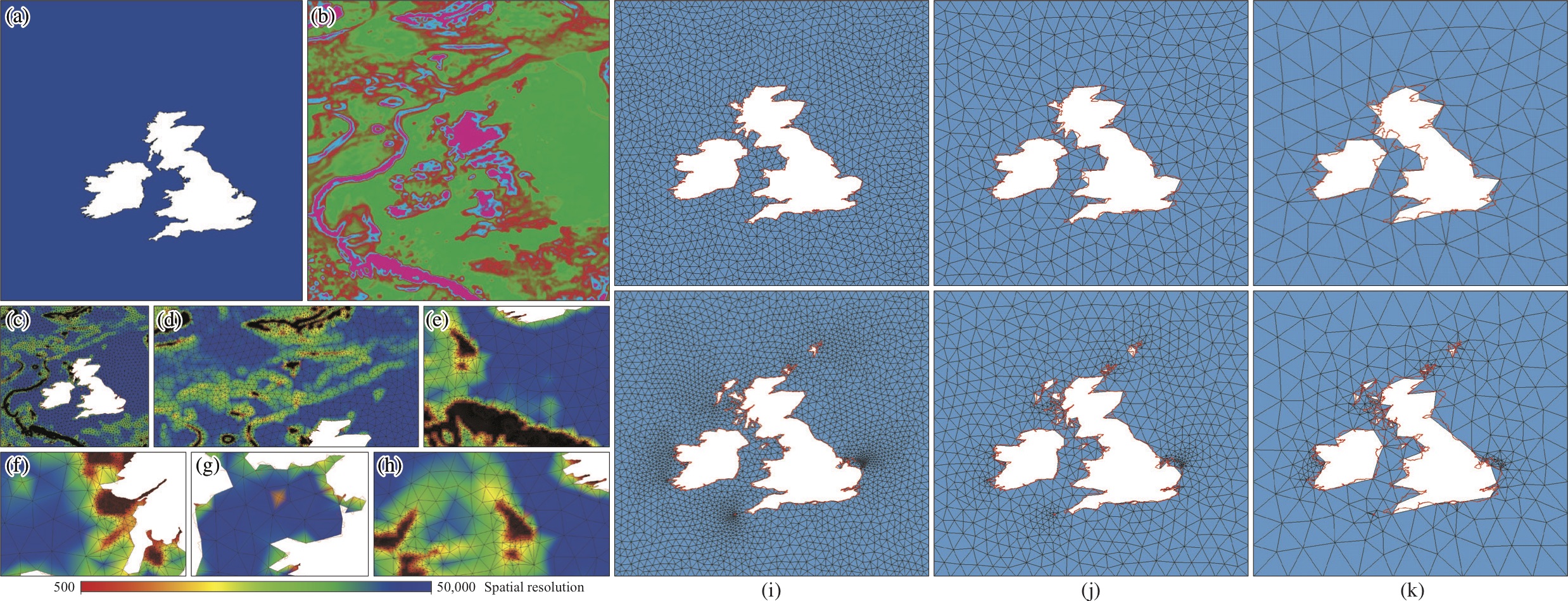
Figure 6: Constraints on the discretization of a UK coastal seas domain containing the two largest land masses of the UK and Ireland, showing (a) a high fidelity BR, and (b) the associated metric $\mathcal{M}_{h}$ based on the sea bed gradient relative to the geoid plane. The resulting spatial discretization, with local resolution highlighted in color, is shown for the full domain in (c) and regions focused on: (d) the Anton Dohrn seamount, (e) the continental shelf and South West Approaches, (f) Hebrides, (g) Liverpool, and (h) Ireland. At the successively coarser background resolutions of (i) $10\mathrm{km}$, (j) $25\mathrm{km}$ and (k) $50\mathrm{km}$, the mesh and discrete coastline generated through a bottom-up approach from a high fidelity BR described by Shingle and shown highlighted in red. The top contains the two largest identified land features, and the bottom the first 49.

To develop the full extruded domain $\mathcal{T}$ (shown in figure 4) from $\mathcal{T}_{h}$, the surface bounds $f$ and $g$ are defined from depth and ice draft fields. The vertical metric function $\mathcal{M}_{v}$ implements a generalized hybrid vertical coordinate (see section 6.4) and contains a specification of $\sigma$-coordinates in ice-covered and coastal regions up to the continental shelf, transitioning to $z-$levels in the open ocean. The extrude to achieve $\{\mathcal{T}_{h},\;f,g,\;\mathcal{M}_{v}\}\mapsto\mathcal{T}$ is performed in parallel, with the geoid discretization $\mathcal{T}_{h}$ divided by ParMetis and distributed in binary format across multiple processors and MPI processes. The associated fields $f$, $g$ and $\mathcal{M}_{v}$ are similarly split, stored efficiently in binary unstructured VTK data types and sent to the corresponding MPI processes. This addresses scalability of item 6, facilitating mesh generation in parallel for geophysical domains and permitting the full discretization of very large multi-scale domains.

Global paleo-oceans

In addition to developing a consistent discretization, the motivation for this work is to enable automated generation to arbitrary geoid bounds. The constraint description developed for figure 4 is easily applied to the Rtopo dataset to include ice shelf ocean cavities in the hydrological domain. Moreover, it is easily extended to modeling ancient seas in domains with bounds that follow and conform to coastlines. Palaeoenvironment reconstructions of global bathymetry utilizing geological observations are used to build domains to ancient coastlines. These are now simple, controllable and methodical modifications to the present day global ocean constraints (figure 4), and with the robust approach, easily applied for a range of ages (figure 5).

7.2 UK coastal seas

A subset of GEBCO in the region $[-14.0,6.0]\times[46.0,64.0]$, for longitude-latitude coordinates ($\psi$,$\phi$) is used to develop the spatial discretization of the UK coastal seas in figure 6(a)–(h). This raw source data has a native resolution of 30 arc seconds, approximately $1\mathrm{km}$ on the geoid plane, and this resolution is maintained for the boundary and metric constraint descriptions. Following figure 2(b) a high-resolution discrete approximation to BR (1) is generated by Shingle along the $0\mathrm{m}$ depth coastline at this native resolution, by solving (10) with $d$ as the function $\mathcal{F}$ and the constant $c=0$, i.e. the path $\Gamma^{\prime}\!:[t_{0},t_{1}]\subset\mathbb{R}\mapsto\xi(t)\in\mathbb{R}^{2},$ for $d(\xi(t))=0$. This BR $\Gamma^{\prime}$ is shown outlined in figure 6(a). An isotropic geoid edge-length metric (2) based on a measure of bathymetry gradient of the form

$$\mathcal{M}_{h}(\boldsymbol{x})\!:\boldsymbol{x}\in\Omega^{\prime}\mapsto\|\nabla d(\boldsymbol{x})\|_{2}=\left(\!\left(\frac{\partial d}{\partial x}\right)^{\!\!2}\!\!+\!\left(\frac{\partial d}{\partial y}\right)^{\!\!2}\right)^{\!1/2}\!\!\!\in\mathbb{R},$$

is developed in figure 6(b) that is consistent with the BR shown in figure 6(a), being also a function of the source GEBCO dataset $d$.

The same high fidelity discrete BR from Shingle of figure 6(a) is paired with a constant spatially homogeneous background geoid edge-length metric (2) of the form: $\mathcal{M}_{h}(\boldsymbol{x})\!:\boldsymbol{x}\in\Omega^{\prime}\mapsto c$, for a constant $c$, to illustrate the bottom-up approach approximating the coastline at a consecutively coarser resolution in figure 6(i)–(k). It is easy to edit contributions to the BR with this approach, and figure 6(i)–(k) also presents meshes from a high fidelity BR containing a larger number of islands.

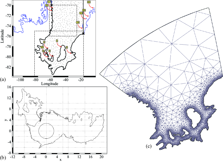
Figure 7: (a) Identification of the Filchner-Ronne ice shelf ocean cavity bounds from RTopo. A total of 348 contours are identified in the SO upto a latitude of 50°S, joined at the 180°W – 180°E meridian, and ordered by size. For example, path 5 outlines Berkner Island that lies between the Filchner and Ronne ice shelf cavities. The dashed lines mark the two specified regions of interest and where paths exit their union the boundary is extended by meridians up to the specified 65°S latitude to be closed automatically by a parallel. The figure shows direct graphical output, with the two meridians and their points of intersection overlaid on top, together with the shading of the output domain, defined by the path orientation. (b) The BR selected in (a) and generated by Shingle, shown under the stereographic projection (12) about the North Pole, in the chart under which the meshing algorithm operates, together with the remaining grounding line contours identified in the SO and closure to the 60°S parallel. (c) Geoid surface mesh that results from the BR development shown in (b), in 3D Euclidean space, presented through an orthographic projection.

7.3 Ice shelf ocean cavity

Domains including ocean cavities that sit below the floating ice shelves of Antarctica are bounded on the geoid plane by grounding lines where ice meets bedrock, coastlines and the open ocean. Immediately these present new challenges to automated, consistent discretization. Grounding line positions are considerably harder to constrain than coastlines, requiring observations from Autonomous Underwater Vehicles (AUV), for example, and tend to see frequent updates, with significant changes. Orientated vector paths of these usually do not exist, or are soon out of date. Additionally, unlike the global oceans, which are bounded only by coastlines, or the UK coastal sea example, which contained only an open ocean boundary, this has a mix of boundary types and identifications. Generation requires interaction with more bespoke datasets, e.g. RTopo or finer resolution data direct from AUV observations.

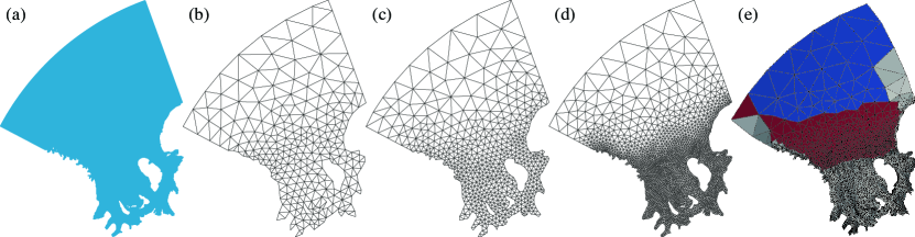
Figure 8: Filchner-Ronne ice shelf region containing the ten largest land masses. (a) High-fidelity BR $\Gamma^{\prime}$ automatically constructed from the grounding line up to the 65^∘S parallel, containing 18,354 control points at a spatial resolution of 500m over a meridional extent of $\sim$1,600km. This is automatically meshed, at three different background mesh metrics $\mathcal{M}_{h}$ from 500km at the bounding parallel down to 100km, 50km and 20km at the grounding line for (b) – (d) respectively. (e) shows a $\textrm{P}_{0}$ (element-wise) identification function, for use in the extrusion to $\mathcal{T}$. All developed in 3D Euclidean space, presented through an orthographic projection about the South Pole.

Filchner-Ronne ice shelf ocean cavity

Filchner-Ronne is the second largest ice shelf in Antarctica (see figure 13), approximately $840\textrm{km}$ long, up to $600\textrm{m}$ thick and covering waters as deep as $1,400\textrm{m}$ at the grounding line. Using the approach described, the domain containing the Filchner-Ronne ice shelf ocean cavity shown in figure 7(a) is straightforwardly captured with the constraints presented in (15). In this case the unfiltered self-consistent RTopo dataset for latitudes from 50°S to the South Pole is loaded and limited to two selected regions described by bounding boxes $[-85.0,-20.0]\times[-89.0,-75.0]$ and $[-67.0,-30.0]\times[-76.0,-70.0]$, for longitude-latitude coordinates ($\psi$,$\phi$).

RTopo includes position data for the coast and grounding lines. However, even those these are consistent with other spatial data within the source, this itself is not sufficient to derive a BR, since points are not grouped, ordered, nor orientated to define the paths required to form (1). Instead the derived region type mask amask field of RTopo is used here directly to identify the ocean part of the surface geoid and a BR that follows the grounding line below the floating ice sheet and coastline where cavities are not present. As outlined in section 3 above, the amask field is filtered in the same way as other Rtopo fields, such as bedrock and ice draft, which are used later for vertical bound constraint. The functional $\mathcal{F}$ of (9) is formed efficiently with a modulo operation on the mask to combine regions identified as open ocean and ice-covered ocean (by integers 0 and 2, respectively), in contrast to the bare bedrock and grounded ice regions (by integers 1 and 3, respectively).

Where the paths are clipped by the bounding region, the domain is automatically extended with meridians up to the 65°S parallel and closed with boundaries identified as open ocean. Figure 7(a) illustrates one of the graphical interfaces which can be used to display the paths identified and their unique label number with regions overlaid, for verification and more accurate selection when needed. The resulting BR is shown in figure 7(b), and subsequent discretization in figure 7(c).

Through the bottom-up approach, figure 8 highlights the ease at which it is possible to construct finer and increasingly better resolved discretizations of the geoid boundary generated by Shingle, in combination with Gmsh. This makes it easy to both draft spatial discretizations themselves, using first coarse approximations during early prototyping stages, and also in the development of a hierarchy of complexity in model simulations, where the level of detail captured is easy to control.

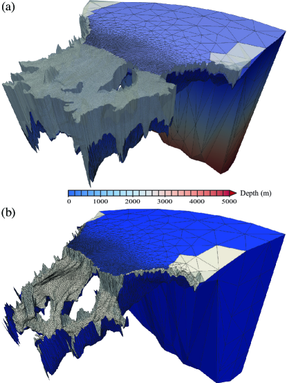
Figure 9: (a) Full discretized domains of the Filchner-Ronne ice shelf ocean cavity and floating ice sheet, conforming to the complex external and internal geometric features and interface surfaces. Vertical extent is radially exaggerated by a factor of 300. (b) Identification function shown to pick out the melting and freezing coupling interface where the ocean meets the floating ice sheet.

In figure 9(a), the full discretized domains of the ocean and floating ice sheets, $\mathcal{T}^{o}$ and $\mathcal{T}^{i}$ respectively are shown, with variable spatial resolution on the geoid. The discrete domains $\mathcal{T}^{o}$ and $\mathcal{T}^{i}$, with vertical bounds $f^{o},g^{o}$ and $f^{i},g^{i}$ respectively, meet exactly at the ice–ocean interface, with

$$g^{o}(\boldsymbol{x})=f^{i}(\boldsymbol{x}),\quad\forall\;\boldsymbol{x}\in{\Gamma^{\prime}}^{i}.$$

Incorporating these coupled interfaces in structured mesh models is relatively easy, and methods and implementations exists. For unstructured-mesh models this is a significant challenge, if one is to ensure the benefits of unstructured approaches are fully leveraged, with accurate conforming boundaries and multi-scale spatial resolution.

Geoid discretization is made on a plane through a stereographic projection to give a curved shell in 3D Euclidean space, which is then extruded to the full discretization $\mathcal{T}$. The curvature of the representation of the 65^∘S parallel in Euclidean space can be seen in figure 9.

Pine Island Glacier ice shelf ocean cavity

Pine Island Glacier (PIG) ice shelf ocean cavity is located in the Amundsen Sea region of West Antarctica (see figure 13) and is significantly smaller and fine scale than cases above. The floating ice sheet is approximately $115\textrm{km}$ long and with the water column below up to around $1\textrm{km}$ deep (figure 10), again with an notably acute aspect ratio.

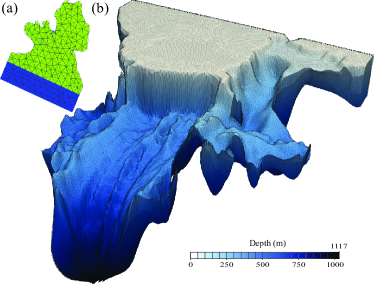
Figure 10: Pine Island Glacier ice shelf ocean cavity, with (a) presenting the consistent high fidelity BR constructed to conform to the grounding and coastlines marked by the self-consistent source dataset. A relatively coarse spatial approximation is shown, with an additional sponge region added and shown in blue. (b) Full discretized domain, at a finer homogeneous geoid resolution, inheriting the self-consistency of the source data fields.

RTopo is relatively coarse at this scale and instead we select a finer dataset generated directly by an observational campaign using an AUV (Autosub 3, built by the UK National Oceanography Centre and deployed by the British Antarctic Survey, Dutrieux et al., 2014). In this case there exists no orientated vector path of the grounding line position, nor of the coastline. From self-consistent ice draft and bedrock positions that have been uniformly filtered, a BR identifying the position of the grounding/coast line is constructed using Shingle. This high fidelity BR is shown in figure 10(a) in a local UTM plane projection, with a relatively coarse spatial discretization $\mathcal{T}_{h}$, colored by its inherited identification from $n_{\Omega^{\prime}}$ which marks where sponge conditions are to be applied in a region accurately bounded by orthodromes. With this coarse spatial approximation, the smaller land masses are not directly represented in the boundary of the resulting geoid discretization. The BR has been clipped along a parallel, and then extended in local UTM space to incorporate a sponge region required for relaxing to open ocean conditions.

Full discretization of the ocean domain is shown in figure 10(b), extruded to the self-consistent fields of bedrock and ice draft. Geoid spatial resolution is homogeneous at approximately $1\textrm{km}$. This resolution is larger than the raw data, so a Gaussian filter is applied throughout to all fields based on this required local spatial resolution. With the domain being built up from a single self-consistent dataset, it is possible to apply this consistently to all sources used in the domain discretization, and notably in the BR such that self-consistency is maintained and the resultant discrete domain is self-consistent.

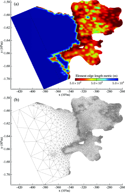
Figure 11: (a) Geoid element edge-length metric $\mathcal{M}_{h}$ based on the local gradient of water column thickness, presented in a local UTM projection. (b) Resulting multi-scale geoid spatial discretization $\mathcal{T}_{h}$, of the Pine Island Glacier ice shelf ocean cavity.

With a relatively high spatial resolution of the source dataset, there is the possibility to optimize the geoid spatial resolution through the metric $\mathcal{M}_{h}$ (2). Figure 11 shows the scalar geoid metric field

$$\mathcal{M}_{h}(\boldsymbol{x})=\mathcal{A}(\|\nabla(g^{o}(\boldsymbol{x})-f^{o}(\boldsymbol{x}))\|),$$

which describes a spatial resolution based on the local change in gradient of water column thickness. The gradient is scaled by $\mathcal{A}$, a simple affine transformation, such that the range of scales varies from $500\textrm{m}$ to $50\textrm{km}$. The resulting geoid discretization contains a higher spatial resolution (for both the 1D boundary and 2D surface discretizations) at the ice front, along the deepest parts of the grounding line, and in the region close to the back where a network of geometrically complex sub-basal channels exist in the floating sheet.

7.4 Southern Ocean

Following discretizations in the small and geometrically complex ice shelf ocean cavities, this section extends this established self-consistent process out to the SO, demonstrating the efficient prototyping, scalability and hierarchy of automation of the approach (items 6, 7 and 9).

A high fidelity BR is produced from the amask field of RTopo, capturing all the land masses of Antarctica. Here the domain contains a large open boundary aligned along a parallel completely circumscribing the globe. The implementation Shingle closes the domain along this free boundary and ensures this is well represented in the output discretization. With the focus on the southern hemisphere, the stereographic projection (12) used in generating $\mathcal{T}_{h}$ is made about a projection point at the North Pole instead of the South.

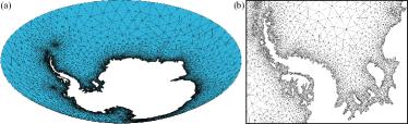
Figure 12: (a) Surface geoid discretization $\mathcal{T}_{h}$ of the ocean domain around Antarctica, with the open bounding parallel extended up to 50°S. The computational domain includes ice shelf ocean cavities and meshing proceeds up to the grounding line, or coastline where no floating ice is present. (b) Zoomed in region, under an orthographic projection, highlighting the small boundary details of the Larsen family and Filchner-Ronne ice shelves, picked up from figure 7.

Figure 13: (a) Full discretized domain $\mathcal{T}$ of the SO up to the land and ice masses of Antarctica is shown, containing the largest 348 land masses of Antarctica, together with the discretized floating ice sheet domains, identified clockwise as (Rs) Ross, (PIG) Pine Island Glacier, (Rn) Ronne, (Fl) Filchner, (L) Larson, (B) Brunt, (Fm) Fimbul, and (A) Amery. These share and each conform to the ice–ocean interface surface. (b) Focused on the West Antarctica region, with the discretized ice shelf domain removed, showing the discretized full domain of the fluid ocean. The large cavities under the Ross and Filchner-Ronne ice sheets are seen to the left and right respectively. (c) A vertical transect through the full discretized domain revealing the generalized hybrid coordinates in the vertical. Region identification $n_{\Omega^{\prime}}^{o}$ made on the geoid marks open ocean, continental shelf and cavity regions, corresponding to $z-$levels, hybrid transition, and $\sigma-$layers colored blue, red and yellow, respectively. (d) View from below highlighting the flexibility in the range of spatial scales and boundary conformity seamlessly captured by the approach in a single multi-scale discretization, in line with the South Pole and (e) towards West Antarctica.

Figure 12 shows the geoid mesh $\mathcal{T}_{h}$ to this conforming bound through the process $h$ 7 of figure 2(b), with a proximity metric to pick up details in coast and grounding line representation. The full discretized domains of the ocean and floating ice sheets, $\mathcal{T}^{o}$ and $\mathcal{T}^{i}$ respectively are shown in figure 13, with variable spatial resolution on the geoid, and generalized hybrid vertical coordinates.

Within $\mathcal{T}_{h}^{o}$ the region identification function $n_{\Omega^{\prime}}^{o}$ demarcates the open ocean, continental shelf seas and cavities covered by a floating shelf. Again, this is at the native resolution of the source dataset like the BR and metric. Generalized hybrid vertical coordinates in $\mathcal{T}$ are developed from $n_{\Omega^{\prime}}^{o}$, with $z-$levels in the open ocean, $\sigma-$layers in the cavities and a smooth transition between the two in the continental shelf sea region.

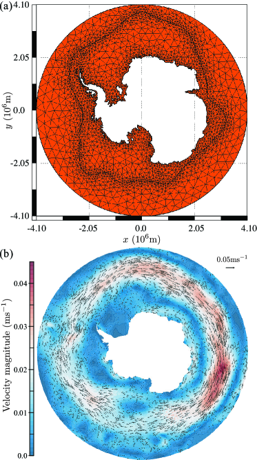
Figure 14: (a) Geoid discretization $\mathcal{T}_{h}$ of the ocean surrounding Antarctica, using the same high fidelity BR as figures 12 and 13, with a geoid metric $\mathcal{M}_{h}$ that is a function of the annual mean track of the Antarctic Circumpolar Current. (b) Surface velocity in the ocean surrounding Antarctica in a simulation performed on a mesh constructed using Shingle. Presented in a polar orthographic projection about the South Pole.

To construct the geoid discretization shown in figure 14(a), a function of the annual mean track of the Antarctic Circumpolar Current (ACC, from Whitworth III, 1988) is trivially included in the functional providing the metric $\mathcal{M}_{h}$ using the Shingle library. This provides a finer spatial resolution along the ACC path, to better represent smaller-scale fluctuations in the ACC compared to a structured, or mesh with homogeneous spatial resolution. To ensure the coastline and grounding lines are well-represented, the metric is additionally a function of proximity to these features.

Figure 14(b) shows an example simulation in a SO domain constructed with this approach. The simulation was performed on a mesh generated from the GEBCO (2014) dataset, does not include ice shelf cavities in this case, using the finite element model Fluidity and the $P_{1}^{\mathrm{DG}}-P_{2}$ velocity – pressure element pairing (Cotter et al., 2009), with the results above shown in a continuous linear space after undergoing a Galerkin projection.

7.5 Ice sheet

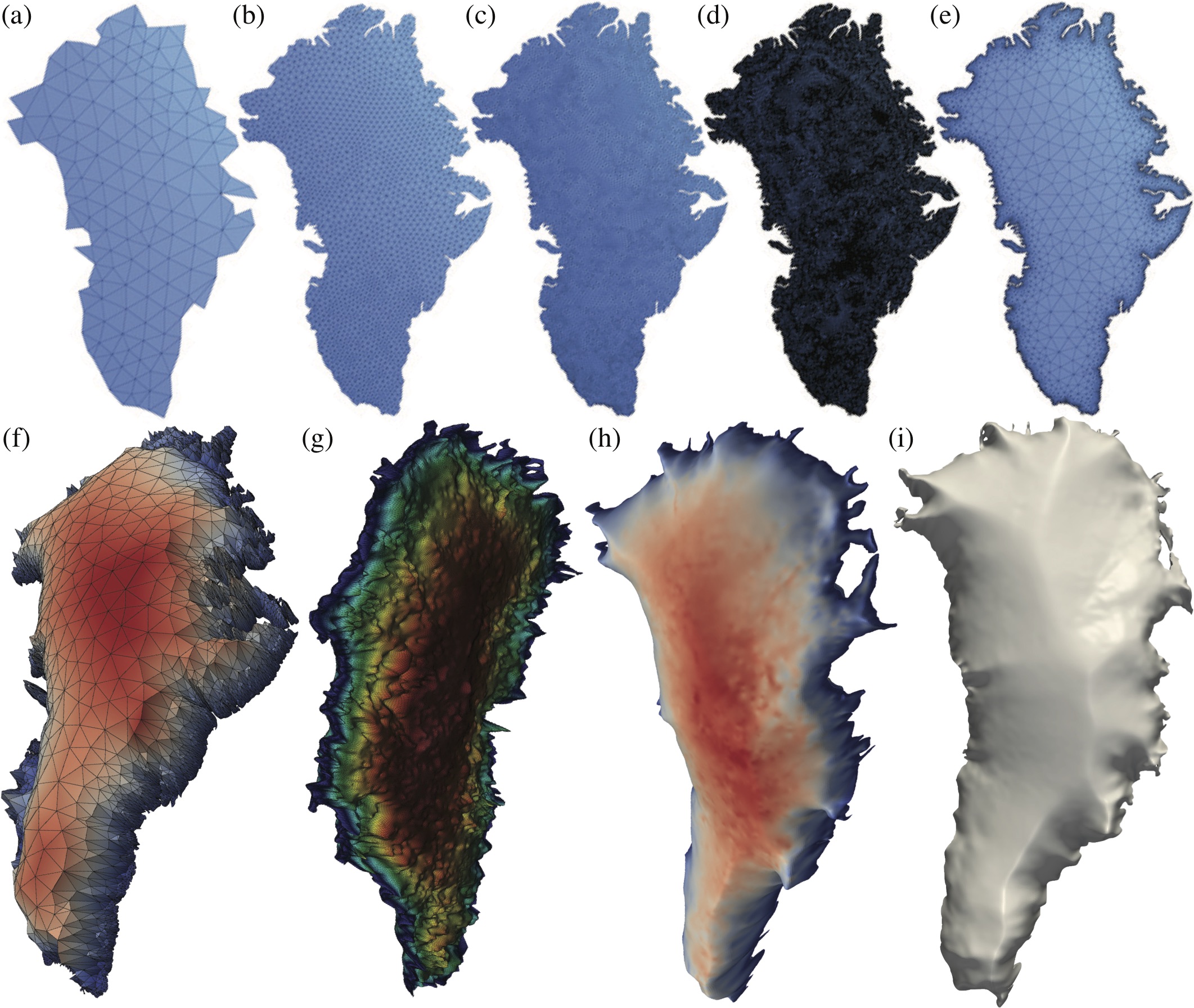
Figure 15: (a)–(e) Automated geoid discretizations of the Greenland ice sheet to a terminating ice sheet thickness of 10m, at successively finer homogeneous spatial resolutions, and a multi-scale discretization ensuring the terminating front is well-represented. Full discretizations of the Greenland ice sheet developed from the $\mathcal{T}_{h}$ of (a)–(e) above, showing ice sheet thickness. Spatial resolutions that are (f) inhomogeneous, (g) 5km homogeneous and 1km in (h) and (i), over a meridional extent of $\sim$2,400km.

The implementation has been applied to the Greenland and full Antarctic ice sheet. In the case of the former, the Greenland Standard Data Set (GSDS, 2011) is the source, using the fields of bed topography, ice thickness and surface elevation (from Bamber, 2001; Jakobsson and et al., 2012). High fidelity surface geoid bounds are defined with the functional $\mathcal{F}$ in (9) of the form

$$\mathcal{F}:=S_{d}(\zeta(t))-S_{b}(\zeta(t)),$$ (14)

where the functions $S_{d}\!:\Omega^{\prime}\mapsto\mathbb{R}$ and $S_{b}\!:\Omega^{\prime}\mapsto\mathbb{R}$ are the ice draft and bedrock bathymetry fields, respectively, from the consistently prepared source dataset. In this case $c$ in (10) is the terminating ice sheet thickness.

The resulting discretized BR at a range of spatial resolutions on the geoid plane, constrained by $\mathcal{M}_{h}$, is shown in figure 15(a)–(e). The full discretized domains (figure 15(f)–(i)) were generated to bounds defined from bed topography and ice thickness fields, with an equal number of sigma layers internally, developed over multiple cores.

These spatial discretizations have been developed for simulations with a 2D Blatter-Pattyn model written in dolfin-adjoint with FEniCS (Farrell et al., 2013) and a 3D full Stokes model (Mouradian, 2015). In both cases, field data required for simulation, such as precipitation and ablation, are interpolated as finite element fields over the constructed spatial discretization, stored and distributed efficiently in parallel VTK unstructured data structures.

Whilst it would be possible to use the GSHHS dataset to generate BRs of both Antarctica and Greenland that include the floating ice sheets up to the ocean interface, it would be difficult to ensure this is consistent with other fields required, or to modify to take into account of newer datasets, or model type. This approach has the option to easily go down to different terminating thicknesses, depending on the simulation model and its complexity. In the case of the single-layer 2D Blatter-Pattyn model, for example, this approach allowed for the efficient development of successively finer spatial approximations from $100\textrm{km}$ down to $1\textrm{km}$ resolution. The latter containing 12,635,550 nodes and 67,253,314 triangular elements, which was used successfully to compute 2D Blatter-Pattyn model simulations on the TACC Stampede Supercomputer.

8 Review of the nine geophysical meshing tenets

Item 1 requiring an accurate description and representation of boundaries $\Gamma^{\prime}$ to a prescribed degree with conforming and aligned faces is not only true of the fractal-like boundaries of the geometrically complex geophysical bounds, but also the smooth domain closures, which under a piecewise-linear approximation require a minimum number of control points to be well-represented locally, with, for example, parallels and meridians represented well enough in stereographic space such that mesh boundaries accurately follow orthodromes in 3D Euclidean space.

Item 2 requires control over spatial resolution, achieved through $\mathcal{M}_{h}$ and $\mathcal{M}_{v}$, functions of the same self-consistent source fields as $\Gamma^{\prime}$ in order to ensure the resulting spatial discretization is consistent. From the high fidelity BR constructed by Shingle, accurate control over the spatial discretization of the boundary is demonstrated, and notably in the PIG case of section 7.3 where a complex geoid metric is developed based on local gradients in surface topographies.

Item 3 requires an accurate geometric specification of regions which is demonstrated in the SO case of section 7.4 through $n_{\Omega^{\prime}}^{o}$ in order to build up generalized hybrid vertical coordinates. Additionally, boundary features are geometrically constrained, such as the sponge region aligned to parallels in the PIG discretization.

Self-consistency in the discretized domain $\mathcal{T}$, covered by item 4, is inherited from self-consistency present in the source data and consistent processing of the approach. As a result there are no issues arising from misalignments, no need for infilling or similar operations, such that node positions and field values are an accurate and faithful representation of the source datasets.

The efficient drafting and prototyping requirement of item 5 is achieved with an automated process from data to spatial discretization. A modeler need only adjust the problem constraints, which are then faithfully adhered to by Shingle and the process figure 2(b), to give the one-one injection initially posed as the challenge in figure 1.

Scalability of item 6 is demonstrated with a range of sized cases considered, from PIG to the global oceans, and with computationally expensive operations sent for distributed processing on HPC resources.

The process is automated, but allows individual elements of the workflow illustrated in figure 2(b) to be adjusted, providing item 7, a hierarchy of automation. Shingle constructs a complete surface geoid domain, closing open boundaries where necessary, but permits finer scale control over constraints where required (see also Candy et al., 2014; Candy and Pietrzak, 2017).

With the injective process, and full description of constraints, the workflow is reproducible and ensures provenance of the discretization development, item 8. Additionally, generation parameters are reproduced alongside the meshing constraints constructed by Shingle, such that generation provenance is recorded.

For the final item 9, standardization of interaction, standard software libraries (see section C), geometric methods (e.g. GDAL, ) and data formats (VTK and Gmsh) are used in the approach to ensure interoperability between both tools and scientists. A new approach solidly handling items 8 and 9 is presented in Candy and Pietrzak (2017).

Conclusion

This paper set out to meet four objectives to work in addressing the new and increasing challenges in taking full advantage of flexible spatial discretizations for multi-scale geophysical simulation, and in a rigorous approach. First providing a concise, formal description of the constrain problem, which is arrived at in section 2.4 and specifically constraints 2. Secondly, to outline the solution requirements for geophysical model domain discretizations, which are detailed in section 2.5 and delivered in table 1. Thirdly, to introduce a consistent approach to the generation of BR, geoid discretization and assembly of a full 3D discretization where necessary. The self-consistent approach is introduced in section 3 and detailed in sections 4, 5 and 6, for the geoid BR, spatial edge-length metric and domain identification, respectively. For the fourth, this enables rigorous unstructured mesh generation in general, and specifically to accurately conform to arbitrary boundaries with only a functional definition where no orientated vector dataset exists.

This research was necessitated by the requirement to construct boundary-conforming unstructured mesh discretizations of ice shelf ocean cavities where it was not possible to use existing tools. In this process the opportunity was taken to address the problem in general for geophysical models, creating the Shingle library, a high-level abstraction to BR generation, to simplify and develop an efficient method, enabling the automated and rigorous construction of conforming boundaries to arbitrary datasets that ensures domain consistency.

Models are advancing from simulating relatively larger-scale flows to include smaller-scale physics in a single seamless process. These small scales bring focus to the boundaries of geophysical models, such that it is important to have accurate control over their representation and importantly, this is consistent with other simulation fields. This demands the consideration and approach introduced, and is a platform for formalized, well-described and accessible routine mesh generation for unstructured mesh models.

A Methods to describe constraints

Relatively simple high-level constraint descriptions can be provided on the command line, with the domain containing the Filchner-Ronne ice shelf ocean cavity shown in figure 7(a) straightforwardly captured with the following

  shingle -n RTopo105b_50S.nc -f Filchner-Ronne.geo

-t rtopoiceshelfcavity -lat -65.0

-b -85.0:-20.0,-89.0:-75.0

$$\texttt{\small{\phantom{-b }-67.0:-30.0,-76.0:-70.0}},$$ (15)

directly acting on a source file provided by Timmermann and et al. (2010). For cases requiring a more complex set of constraints, the flexible, extensible approach described in Candy and Pietrzak (2017) is appropriate. This uses natural language, geophysical feature based objects in a hierarchical constraint-complete description, that is model-independent for sharing in general.

B Simulation time-varying spatial discretization

Domain bounds and resolution metrics can be initialized from the outset to describe a discretized domain that best captures the dynamics for an entire simulation. With a runtime adaptive algorithm, the initial domain discretization can be focused on best representing the initial conditions and coupling pathways, with the discretization then evolving in response to solution dynamics and coupling requirements. For domains in geophysical simulations, the first time-varying extension is to allow the resolution metrics (2) and (6) to vary in time, i.e. ${\partial\mathcal{M}_{h}(\boldsymbol{x},t)}/{\partial t}\neq 0$ and ${\partial\mathcal{M}_{v}(\boldsymbol{x},t)}/{\partial t}\neq 0$, for $\boldsymbol{x}\in\Omega$ over the time interval $[0,\textrm{T})$, whilst 1, 3, 4 and 5 remain fixed. This redistribution of spatial resolution can be achieved with relatively efficient $r-$ and $h-$ adaptive processes. The distinction in spatial directions that decouples the domain discretization needs to be preserved throughout the simulation, such that it is possible to regenerate $\mathcal{T}_{h}$ and then $\mathcal{T}$, evaluating the contribution of $\mathcal{M}_{h}$ and $\mathcal{M}_{v}$ through the processes 7 and 8 respectively. This requires that the distinction is registered with the model code such that nodes are identified to gravitationally aligned columns, with information of the discretization $\mathcal{T}_{h}$ propagated to $\mathcal{T}$. During model simulation on multiple processors, in the global ocean, ice shelf ocean cavity, ACC and SO simulations presented, the domain mesh of is collapsed to the geoid surface mesh through an inverse prolongation operation (e.g. Kramer et al., 2010), and optimized with a 2D adaptive algorithm (such as Lipnikov and Vassilevski, 2004), following the evolving $\mathcal{M}_{h}$. From this surface geoid mesh $\mathcal{T}_{h}$, the full mesh is built up through an extrusion processes to $f$ and $g$ following $\mathcal{M}_{v}$.

The next extension is to additionally permit the vertical bounds (5) to vary in time. This is applied in the ice shelf ocean cavity simulations. The top surface $g$, that describes the continuous ice–ocean and air-ocean boundary, adjusts in time in response to changes in pressure within the cavity, whilst the bottom bound $f$, describing ocean bathymetry, remains fixed. Conservation of mass and component physical models introduce further constraints on how the domain surface is modified. The vertical coordinate system is adjusted in time following $n_{\Omega^{\prime}}$ changes, to ensure an optimal spatial discretization, with primitives conserved following Farrell et al. (2009).

The final extension is to allow the geoid plane BR (1) to vary in time. In practice it is a computationally expensive process, and other approaches are more efficient in adjusting extent on the geoid plane, such as activating regions with wetting-and-drying procedures (e.g. Candy, 2017).

Permanence of boundary representation

An arbitrary repositioning or change in node number within $\mathcal{T}_{h}$, with a subsequent extrusion through $f$ and $g$, does not ensure a conservation of volume. A simple approach which permits refinement, is to begin with a coarse $\mathcal{M}_{h}$ and associated $\mathcal{T}_{h}$, whose nodes remain in the discretization throughout a simulation, with extrusion bounds $f$ and $g$ for any refinements determined by linear interpolation. In this approach the representation of the surface boundary is selected at initialization and not refined during a simulation in order to conserve volume.

C Standardization of interaction

The approach is realized in the implementation Shingle, a software library which is written in Python, a widely used high-level, interpreted programming language that has been designed to be highly extensible. Python has a small core, with a large standard library and an easily extensible interpreter, making it easy to build up individual components in a hierarchy of automation (item 7).

It relies on established, well-regarded libraries for standard numeric operations (including NumPy, SciPy (Oliphant, 2007) and Matplotlib) and geospatial libraries for robust projection and geometric operations (including GDAL , GMT , NetCDF, shapefile, and PROJ.4 ). Scalability built into these is inherited by the approach (item 6). In order to quickly prototype BRs identified in (10), computationally demanding solutions can be cached to disk in a compact binary representation using the standard Python pickle library.

Distribution and sharing of spatial discretization constraints for model intercomparisons, data provenance and a consistency between model setups is addressed in Candy and Pietrzak (2017). Since geophysical spatial discretizations can be reproduced in an automated deterministic way using the interpreter Shingle, it is also sufficient and constraint-complete to depend on the self-consistent source data in a standardized format and processing record: of pre-processing operations applied using standard common geospatial tools, the BR generation operation such as (15) and metric formulae with reference to the interpretors Shingle and Gmsh.

References

- Bamber (2001) Bamber, J., 2001. Greenland 5km DEM, ice thickness, and bedrock elevation grids, Version 1.
- de Brye (2011) de Brye, B., 2011. Multiscale Finite-Element Modelling of River-Sea Continua. Ph.D. thesis. Institut de Mécanique, Matériaux et génie Civil, Université Catholique de Louvain.
- Candy (2017) Candy, A., 2017. An implicit wetting and drying approach for non-hydrostatic baroclinic flows in high aspect ratio domains. Adv. Water Resour. 102, 188 – 205.
- Candy et al. (2014) Candy, A.S., Avdis, A., Hill, J., Gorman, G.J., Piggott, M.D., 2014. Integration of Geographic Information System frameworks into domain discretisation and meshing processes for geophysical models. Geosci. Model Dev. Discuss. 7, 5993–6060.
- Candy and Pietrzak (2017) Candy, A.S., Pietrzak, J.D., 2017. Shingle 2.0: generalising self-consistent and automated domain discretisation for multi-scale geophysical models. In review .
- Casarotti et al. (2008) Casarotti, E., Stupazzini, M., Lee, S., Komatitsch, D., Piersanti, A., Tromp, J., 2008. GEOCUBIT, an HPC parallel mesher for spectral-element method seismic wave simulation. SPE, EAGE .
- Chen et al. (2003) Chen, C., Liu, H., Beardsley, R.C., 2003. An unstructured grid, finite-volume, three-dimensional, primitive equations ocean model: Application to coastal ocean and estuaries. J. Atmos. Oceanic Tech. 20, 159–186.
- COMSOL (2016) COMSOL, 2016. Comsol multiphysics. http://www.comsol.com.
- Cotter and Gorman (2008) Cotter, C., Gorman, G., 2008. Diagnostic tools for 3d unstructured oceanographic data. Ocean Modell. 20, 170 – 182.
- Cotter et al. (2009) Cotter, C., Ham, D., Pain, C., Reich, S., 2009. LBB stability of a mixed Galerkin finite element pair for fluid flow simulations. J. Comput. Phys. 228, 336–348.
- CUBIT Development Team and Jankovich (2014) CUBIT Development Team, Jankovich, S.R., 2014. CUBIT Mesh Generation Environment Volume 1: Users Manual.
- Cui (2013) Cui, H., 2013. A new numerical model for simulating the propagation of and inundation by tsunami waves. Ph.D. thesis. Delft University of Technology.
- Danilov (2013) Danilov, S., 2013. Ocean modeling on unstructured meshes. Ocean Modell. 69, 195–210.
- Danilov et al. (2008) Danilov, S., Wang, Q., Losch, M., Sidorenko, D., Schröter, J., 2008. Modeling ocean circulation on unstructured meshes: comparison of two horizontal discretizations. Ocean Dyn. 58, 365–374.
- Danilov et al. (2013) Danilov, S., Wang, Q., Sidorenko, D., Timmermann, R., Wekerle, C., Haid, V., Wang, X., 2013. Multiresolution modeling of large-scale ocean circulation, ECMWF Seminar on Num. Meth. for Atmos. and Ocean Modell.
- Deltares (2017) Deltares, 2017. D-Flow FM Technical Reference Manual. Deltares, Delft. URL: https://www.deltares.nl/en/software/delft3d-flexible-mesh-suite. 1.1.0, rev 48665.
- Douglas and Peucker (1973) Douglas, D.H., Peucker, T.K., 1973. Algorithms for the reduction of the number of points required to represent a digitized line or its caricature. Cartographica: Int. J. Geograph. Info. Geovis. 10, 112–122.
- Dutrieux et al. (2014) Dutrieux, P., Stewart, C., Jenkins, A., Nicholls, K.W., Corr, H.F.J., Rignot, E., Steffen, K., 2014. Basal terraces on melting ice shelves. Geophys. Res. Lett. 41, 5506–5513.
- Farrell et al. (2009) Farrell, P., Piggott, M., Pain, C., Gorman, G., Wilson, C., 2009. Conservative interpolation between unstructured meshes via supermesh construction. Comp. Meth. Appl. Mech. Engrg. 198, 2632–2642.
- Farrell et al. (2013) Farrell, P.E., Ham, D.A., Funke, S.W., Rognes, M.E., 2013. Automated derivation of the adjoint of high-level transient finite element programs. SIAM J. Sci. Comput. 35, C369–C393.
- Ford et al. (2004) Ford, R., Pain, C.C., Piggott, M.D., Goddard, A.J.H., de Oliveira, C.R.E., Umpleby, A.P., 2004. A nonhydrostatic finite-element model for three-dimensional stratified oceanic flows. Part I: Model formulation. Mon. Weath. Rev. 132, 2816–2831.
- (22) GDAL, . Geospatial data abstraction library. http://gdal.org.
- GEBCO (2014) GEBCO, 2014. General Bathymetric Chart of the Oceans (GEBCO). http://www.gebco.net.
- George and Borouchaki (1998) George, P., Borouchaki, H., 1998. Delaunay Triangulation and Meshing: Application to Finite Elements. BH.
- Geuzaine and Remacle (2009) Geuzaine, C., Remacle, J.F., 2009. Gmsh: A 3-d finite element mesh generator with built-in pre- and post-processing facilities. Internat. J. Numer. Meth. Eng. 79, 1309–1331.
- (26) GiD, . A universal, adaptive and user-friendly pre and postprocessor for numerical simulations in science and engineering. http://gid.cimne.upc.edu.
- (27) GMT, . Generic Mapping Tools. URL: http://gmt.soest.hawaii.edu. Released under the GNU GPL.
- Gorman et al. (2007) Gorman, G., Piggott, M., Pain, C., 2007. Shoreline approx. for unstructured mesh generation. Comput. & Geosci. 33, 666–677.
- Gorman et al. (2006) Gorman, G., Piggott, M., Pain, C., de Oliveira, C., Umpleby, A., Goddard, A., 2006. Optimisation based bathymetry approximation through constrained unstructured mesh adaptivity. Ocean Modell. 12, 436–452.
- Gorman et al. (2008) Gorman, G., Piggott, M., Wells, M., Pain, C., Allison, P., 2008. A systematic approach to unstr. mesh generation for ocean modell. using GMT and Terreno. Comput. & Geosci. 34, 1721–1731.
- Gourgue et al. (2013) Gourgue, O., Baeyens, W., Chen, M., de Brauwere, A., de Brye, B., Deleersnijder, E., Elskens, M., Legat, V., 2013. A depth-averaged two-dimensional sediment transport model for environmental studies in the scheldt estuary and tidal river network. J. Mar. Sys. 128, 27–39.
- Gourgue et al. (2009) Gourgue, O., Comblen, R., Lambrechts, J., Kärnä, T., Legat, V., Deleersnijder, E., 2009. A flux-limiting wetting-drying method for finite-element shallow-water models, with application to the scheldt estuary. Adv. Water Resour. 32, 1726–1739.
- Greenberg et al. (2005) Greenberg, D.A., Shore, J.A., Page, F.H., Dowd, M., 2005. A finite element circulation model for embayments with drying intertidal areas and its application to the Quoddy region of the Bay of Fundy. Ocean Modelling 10, 211–231.
- Griffies et al. (2005) Griffies, S., Gnanadesikan, A., Dixon, K.W., Dunne, J., Gerdes, R., Harrison, M.J., Rosati, A., Russell, J., Samuels, B.L., Spelman, M.J., et al., 2005. Formulation of an ocean model for global climate simulations. Ocean Sci. 1, 45–79.
- Griffies and et al. (2014) Griffies, S.M., et al., 2014. An assessment of global and regional sea level for years 1993–2007 in a suite of interannual CORE-II simulations. Ocean Modell. 78, 35 – 89.
- Griffies et al. (2000) Griffies, S.M., Böning, C., Bryan, F.O., Chassignet, E.P., Gerdes, R., Hasumi, H., Hirst, A., Treguier, A.M., Webb, D., 2000. Dev. in ocean climate modell. Ocean Modell. 2, 123 – 192.
- GSDS (2011) GSDS, 2011. Greenland Standard Data Set. URL: http://websrv.cs.umt.edu/isis/index.php/Present_Day_Greenland.
- Hagen (2014) Hagen, E., 2014. Hydrodynamic river modelling with D-Flow Flexible Mesh: case study of the side channel at Afferden and Deest. Master’s thesis. University of Twente.
- Haidvogel and Beckmann (1999) Haidvogel, D.B., Beckmann, A., 1999. Numerical ocean circulation modeling. volume 2. World Scientific.
- Ham et al. (2009) Ham, D.A., Pain, C.C., Hanert, E., Pietrzak, J., Schröter, J., 2009. Special Issue: 6th Int. workshop on unstructured mesh numerical modelling of coastal, shelf and ocean flows. Imperial College London, Sep. 19–21, 2007. Ocean Modell. 28, 1 –.
- Hanert (2004) Hanert, E., 2004. Towards a Finte Element Ocean Circulation Model. Ph.D. thesis. Université Catholique De Louvain.
- Holt et al. (2017) Holt, J., Hyder, P., Ashworth, M., Harle, J., Hewitt, H.T., Liu, H., New, A.L., Pickles, S., Porter, A., Popova, E., Allen, J.I., Siddorn, J., Wood, R., 2017. Prospects for improving the representation of coastal and shelf seas in global ocean models. Geosci. Model Dev. 10, 499–523.
- Humbert et al. (2009) Humbert, A., Kleiner, T., Mohrholz, C.O., Oelke, C., Greve, R., Lange, M.A., 2009. A comparative modeling study of the Brunt Ice Shelf/Stancomb-Wills Ice Tongue system, East Antarctica. J. Glaciol. 55, 53–65.
- IMUM (2016) IMUM, 2016. The 15th International workshop on Multi-scale (Un)-structured mesh numerical Modeling for coastal, shelf, and global ocean dynamics, Midi-Pyrénées Observatory, Toulouse, France, 27–30 Sep 2016. https://imum2016.sciencesconf.org.
- Jakobsson and et al. (2012) Jakobsson, M., et al., 2012. The international bathymetric chart of the Arctic Ocean (IBCAO) version 3.0. Geophy. Res. Lett. 39.
- Kantha and Clayson (2000) Kantha, L.H., Clayson, C.A., 2000. Numerical Models of Oceans and Oceanic Processes. Academic Press. Edited by Renata Dmowska, James R. Holton and H. Thomas Rossby.
- Kärnä et al. (2011) Kärnä, T., de Brye, B., Gourgue, O., Lambrechts, J., Comblen, R., Legat, V., Deleersnijder, E., 2011. A fully implicit wetting-drying method for DG-FEM shallow water models, with an application to the scheldt estuary. Comp. Meth. Appl. Mech. Engrg. 200, 509–524.
- Kramer et al. (2010) Kramer, S., Cotter, C., Pain, C., 2010. Solving the Poisson equation on small aspect ratio domains using unstructured meshes. Ocean Modell. 35, 253–263.
- Lambrechts et al. (2008) Lambrechts, J., Comblen, R., Legat, V., Geuzaine, C., Remacle, J.F., 2008. Multiscale mesh generation on the sphere. Ocean Dyn. 58, 461–473.
- Lambrechts and Seny (2011) Lambrechts, J., Seny, B., 2011. Gmsh workshop: Ocean.
- Legrand et al. (2007) Legrand, S., Deleersnijder, E., Delhez, E., Legat, V., 2007. Unstructured, anisotropic mesh generation for the northwestern European continental shelf, the continental slope and the neighbouring ocean. Contin. Shelf Res. 27, 1344–1356.
- Legrand et al. (2000) Legrand, S., Legat, V., Deleersnijder, E., 2000. Delaunay mesh generation for an unstructured-grid ocean general circulation model. Ocean Modell. 2, 17–28.
- Lipnikov and Vassilevski (2004) Lipnikov, K., Vassilevski, Y., 2004. On control of adaptation in parallel mesh generation. Eng. Comput. 20, 193–201.
- Lyard et al. (2006) Lyard, F., Lefevre, F., Letellier, T., Francis, O., 2006. Modelling the global ocean tides: modern insights from FES2004. Ocean Dyn. 56, 394–415.
- Maddison et al. (2011) Maddison, J.R., Marshall, D., Pain, C.C., Piggott, M.D., 2011. Accurate representation of geostrophic and hydrostatic balance in unstructured mesh finite element ocean modelling. Ocean Modell. 39, 248–261.
- Marshall et al. (1997) Marshall, J., Hill, C., Perelman, L., Adcroft, A., 1997. Hydrostatic, quasi-hydrostatic, and nonhydrostatic ocean modeling. J. Geophys. Res. Oceans 102, 5733–5752.
- Meehl et al. (2007) Meehl, G.A., Covey, C., Taylor, K.E., Delworth, T., Stouffer, R.J., Latif, M., McAvaney, B., Mitchell, J.F.B., 2007. THE WCRP CMIP3 multimodel dataset: A new era in climate change research. Bull. Amer. Meteo. Soc. 88, 1383–1394.
- Mouradian (2015) Mouradian, S., 2015. Simulating ice processes using the finite element, unstructured, adaptive model Fluidity. Ph.D. thesis. Imperial College London.
- Nurser (2012) Nurser, G., 2012. Personal communication.
- Oliphant (2007) Oliphant, T.E., 2007. Python for scientific computing. Comput. Sci. Eng. 9, 10–20.
- Pain et al. (2005) Pain, C., Piggott, M., Goddard, A., Fang, F., Gorman, G., Marshall, D., Eaton, M., Power, P., de Oliveira, C., 2005. 3D unstructured mesh ocean modelling. Ocean Modell. 10, 5–33.
- Piggott et al. (2005) Piggott, M., Pain, C., Gorman, G., Power, P., Goddard, A., 2005. h, r, and hr adaptivity with applications in numerical ocean modelling. Ocean Modell. 10, 95–113.
- Piggott et al. (2008) Piggott, M.D., Gorman, G.J., Pain, C.C., Allison, P.A., Candy, A.S., Martin, B.T., Wells, M.R., 2008. A new computational framework for multi-scale ocean modelling based on adapting unstructured meshes. Int. J. Numer. Meth. Fl. 56, 1003–1015.
- (64) PROJ.4, . Cartographic Projections Library PROJ.4. URL: http://www.proj4.org. Released under an MIT license.
- Rebay (1993) Rebay, S., 1993. Efficient unstructured mesh generation by means of Delaunay triangulation and Bowyer-Watson algorithm. J. Comput. Phys. 106, 125 – 138.
- van Scheltinga et al. (2010) van Scheltinga, A.D.T., Myers, P.G., Pietrzak, J.D., 2010. A finite element sea ice model of the Canadian Arctic Archipelago. Ocean Dyn. 60, 1539–1558.
- Sein et al. (2016) Sein, D.V., Danilov, S., Biastoch, A., Durgadoo, J.V., Sidorenko, D., Harig, S., Wang, Q., 2016. Designing variable ocean model resolution based on the observed ocean variability. J. Adv. Model. Earth Sys. 8, 904–916.
- Shewchuk (2002) Shewchuk, J.R., 2002. Delaunay refinement algorithms for triangular mesh generation. Comput. Geom. 22, 21–74.
- Shingle (2011–2017) Shingle, 2011–2017. Computational research software library for high-level abstraction to spatial discretisation of geophysical domains. http://shingleproject.org, library repository at http://github.com/adamcandy/Shingle.
- Sidorenko et al. (2011) Sidorenko, D., Wang, Q., Danilov, S., Schröter, J., 2011. FESOM under coordinated ocean-ice reference experiment forcing. Ocean Dyn. 61, 881–890.
- Snyder (1987) Snyder, J.P., 1987. Map projections – A working manual. volume 1395. US Gov. Printing Office.
- Taylor et al. (2012) Taylor, K.E., Stouffer, R.J., Meehl, G.A., 2012. An overview of CMIP5 and the experiment design 93, 485–498.
- Thomas et al. (2014) Thomas, C.J., Lambrechts, J., Wolanski, E., Traag, V.A., Blondel, V.D., Deleersnijder, E., Hanert, E., 2014. Numerical modelling and graph theory tools to study ecological connectivity in the Great Barrier Reef. Eco. Modell. 272, 160–174.
- Timmermann and et al. (2010) Timmermann, R., et al., 2010. A consistent data set of Antarctic ice sheet topography, cavity geometry, and global bathymetry. Earth System Science Data 2, 261–273.
- Triangle Library Python Bindings (2014) Triangle Library Python Bindings, 2014. https://github.com/drufat/triangle.
- (76) VTK, . The Visualization Toolkit. URL: http://www.vtk.org.
- Wells et al. (2010) Wells, M.R., Allison, P.A., Piggott, M.D., Hampson, G.J., Pain, C.C., Gorman, G.J., 2010. Tidal model of an ancient tide - dominated seaway, Part 1: Model validation and application to global early Cretaceous (Aptian) tides. J. Sed. Res. 80, 393–410.
- Wessel and Smith (1996) Wessel, P., Smith, W.H.F., 1996. A global, self-consistent, hierarchical, high-resolution shoreline database. J. Geophys. Res. 101, 8741–8743.
- Westerink and et al. (2008) Westerink, J., et al., 2008. A basin to channel scale unstructured grid hurricane storm surge model applied to Southern Louisiana. Mon. Weath. Rev. 136, 833–864.
- White et al. (2008) White, L., Deleersnijder, E., Legat, V., 2008. A three-dimensional unstructured mesh finite element shallow-water model, with application to the flows around an island and in a wind-driven, elongated basin. Ocean Modell. 22, 26–47.
- Whitworth III (1988) Whitworth III, T., 1988. The Antarctic Circumpolar Current. Oceanus 31, 53–58.