Kramers problem for a dimer: effect of noise correlations

Abstract

Kramers problem for a dimer in a bistable piecewise linear potential is studied in the presence of correlated noise processes. The distribution of first passage times from one minima to the basin of attraction of the other minima is found to have exponentially decaying tails with the parameter dependent on the amount of correlation and the coupling between the particles. Strong coupling limit of the problem is analyzed using adiabatic elimination, where it is found that the initial probability density relaxes towards stationary value on the same time scale as the mean escape time. The implications towards polymer dynamics in a potential are discussed.

I Introduction

Escape of a particle confined in a metastable state is a ubiquitous problem arising in domains varying from chemical kinetics to transport theory. The theory of Brownian motion provides one of the most elegant approaches to study the problem by identifying the additional degrees of freedom as noise and friction hanggi . This approach towards the escape problem was grounded in the seminal work of Kramers kramers ; talkner , who provided theoretical estimates for the rate of escape for a particle trapped in a metastable state in the limits of low and high friction.

Generalizing the single particle problem, thermally activated escape of extended objects like polymers has attracted attention in recent times mesfin ; park ; lee ; sebastian . The studies have concluded that the escape of a polymer chain from a potential well depends nontrivially on the structural properties of the polymer, viz. the number of monomers constituting the chain and the strength of inter-particle interactions. The results provide a handle to control the rates of chemical reactions involving polymers by varying their structural parameters. Recently the problem of a dimer crossing a potential barrier has been investigated asfaw conforming with the previous results for polymers. However, all these studies have focused on uncorrelated noise processes, whereas it is known that noises from identical origin are generally correlated fulinski . Such correlations significantly affect the dynamics of a particle in a bistable potential jia ; li ; mei ; xie , and are known to induce nonzero transport in periodic potentials due to symmetry breaking sang . The observations motivate us to study the effect of noise correlations on the dynamics of extended objects.

In this paper we study the dynamics of the simplest extended object, a dimer: two harmonically coupled Brownian particles in a piecewise linear bistable potential. Additional thermal degrees of freedom are Gaussian white and correlated with each other. It is found that positively correlated noise processes facilitate barrier crossing for the dimer whereas negative correlations tend to diminish the effect of thermal degrees of freedom. The structure of the paper is as follows: in the next section the effect of coupling and correlation are studied on the motion of the dimer. Following it the strong coupling limit of the dynamics is analyzed and the effects of periodic forcing are also reported. The results are generalized to the dynamics of a polymer in a potential field with conclusions in the final section.

II Dynamical system

Let us start with the dynamical equations for a dimer in a bistable potential $U$:

$$\dot{x}_{1} =-U^{\prime}(x_{1})+F_{12}(x_{1},x_{2})+\eta_{1}(t),$$ (1a)

$$\dot{x}_{2} =-U^{\prime}(x_{2})+F_{21}(x_{1},x_{2})+\eta_{2}(t),$$ (1b)

where $\eta_{1}$ and $\eta_{2}$ are Gaussian white noises of mean zero and correlations:

$$\langle\eta_{1}(t)\eta_{1}(t^{\prime})\rangle =\langle\eta_{2}(t^{\prime})\eta_{2}(t)\rangle=2D\delta(t-t^{\prime}),$$ (2a)

$$\langle\eta_{1}(t)\eta_{2}(t^{\prime})\rangle =\langle\eta_{1}(t^{\prime})\eta_{2}(t)\rangle=2D\rho\delta(t-t^{\prime}),$$ (2b)

with $D$ being the noise intensity and $\rho\in[-1,1]$ the measure of correlation. The noise intensity is a measure of the dimensionless temperature of the associated heat bath. Consequently, the existence of a correlation between the two noise processes is natural as $\eta_{1}$ and $\eta_{2}$ have the same thermal origin. The potential $U$ in eqn(1) is a piecewise linear function defined as:

$$U(x)=\begin{cases}-x-1~{}~{}\text{for}~{}~{}x<-1,\\ x+1~{}~{}\text{for}~{}~{}-1\leq x\leq 0,\\ -x+1~{}~{}\text{for}~{}~{}0\leq x\leq 1,\\ x-1~{}~{}\text{for}~{}~{}x>1,\end{cases}$$ (3)

having global minima at $x=\pm 1$ and a local maxima at $x=0$. Components of the dimer interact via a harmonic potential $U_{sh}=\frac{k}{2}(x_{1}-x_{2})^{2}$, with the corresponding forces $F_{ij}(x_{1},x_{2})=-\frac{\partial}{\partial x_{i}}U_{sh}(x_{1},x_{2})$ with $i\in\{1,2\}$ and $i\neq j$, and $k$ being the spring constant. It is noted that the natural length of the spring is chosen to be negligibly small as compared to the separation of the global minima of the potential $U$ and hence, is ignored in the definition of the interaction potential $U_{sh}$.

In order to diagonalize the correlation matrix in (2), let us transform the dynamical equations to $x_{c}=\frac{x_{1}+x_{2}}{2}$ and $x_{r}=\frac{x_{1}-x_{2}}{2}$, which are respectively the coordinates of the center of mass and relative separation between the two particles. In terms of the variables $x_{c}$ and $x_{r}$, the dynamical equations in (1) are transformed as:

$$\dot{x}_{c} =-\frac{U^{\prime}(x_{c}+x_{r})+U^{\prime}(x_{c}-x_{r})}{2}+\zeta_{c}(t),$$ (4a)

$$\dot{x}_{r} =-\frac{U^{\prime}(x_{c}+x_{r})-U^{\prime}(x_{c}-x_{r})}{2}-2kx_{r}+\zeta_{r}(t),$$ (4b)

where $\zeta_{c}=\frac{\eta_{1}+\eta_{2}}{2}$ and $\zeta_{r}=\frac{\eta_{1}-\eta_{2}}{2}$ are independent noise processes with mean zero and correlations:

$$\langle\zeta_{c}(t)\zeta_{c}(t^{\prime})\rangle =D(1+\rho)\delta(t-t^{\prime}),$$ (5a)

$$\langle\zeta_{r}(t)\zeta_{r}(t^{\prime})\rangle =D(1-\rho)\delta(t-t^{\prime}).$$ (5b)

The stochastic differential equations in (4) and (5) are solved numerically using Heun’s method toral with the initial conditions $(x_{c},x_{r})=(-1.0,0.02)$.

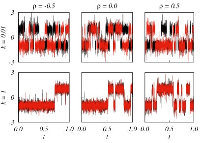
Figure 1: Sample trajectories of the dimer $x_{1}$(black) and $x_{2}$(red) in the piecewise linear bistable potential $U$, with the particles interacting simple harmonically for the initial conditions $(x_{c},x_{r})=(-1.0,0.02)$ for different values of spring constant $k$ and noise correlation $\rho$ for noise intensity $D=0.25$. The time $t$ in the figure is in multiples of $10^{3}$.

Fig. 1 shows the trajectories of the dimer in the bistable potential $U$ for varying correlations $\rho$ and spring constant $k$ for noise intensity $D=0.25$. The dependence of the nature of trajectories on the spring constant $k$ is evident from the figure. For low $k$ the two particles move nearly independent of each other, but for high $k$ the dimer moves as an effective single particle with the two particles fluctuating about the mean position independent of the value of noise correlation $\rho$. However, $\rho$ plays a decisive role in the dimer crossing the potential barrier when the coupling between the monomers is high, with positive correlation aiding in the back and forth hoping between the two minima and the negative $\rho$ confining the monomer in the stable position. To quantify the above observations let us study the residence time statistics of the center of mass in the potential wells, which identifies with the statistics of escape times choi .

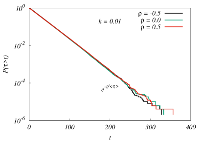
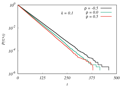
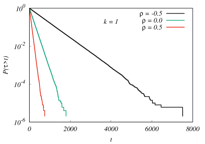
Figure 2: Cumulative distribution of the first passage times $\tau$ of the center of mass starting in the left well to the absorbing boundary at $x_{c}=0$. The distribution has exponentially decaying tails with parameter $\langle\tau\rangle$. The effect of the coupling between the two monomers is evident on the nature of the distribution: for nearly independent movement of the particles($k=0.01$)(top) the distributions trace each other for different values of $\rho$. When the coupling between the monomers increases, the mean first passage time $\langle\tau\rangle$ is found to decrease with increasing $\rho$ as observed for $k=0.1$(middle) and $k=1$(bottom). The distributions are calculated using 500000 data points for noise intensity $D=0.25$.

With the initial condition $x_{c}=-1$, lets look at the time it takes for the center of mass to reach the basin of attraction of the minima at $x_{c}=1$. Fig. 2 shows the distribution of first passage times $\tau$ for different values of noise correlation $\rho$ and spring constant $k$ for noise intensity $D=0.25$. The distribution shows exponentially decaying tails with parameter $\langle\tau\rangle$, the mean first passage time. However, when the coupling between the monomers is low($k=0.01$), $\langle\tau\rangle$ is nearly independent of the correlation $\rho$. This is because for such low values of spring constant $k$, the particles move nearly independent of each other and hence the correlation between the thermal degrees of freedom does not have any significant impact on the rate of barrier crossing of the nearly independent particles. On the other hand, with increasing values of spring constant, e.g.- $k=0.1~{}\text{and}~{}1$, it is observed that $\langle\tau\rangle$ decreases with increasing correlation $\rho$. The reason for such a behavior follows from the dynamical equations in (4) and (5) which imply that the noise intensity affecting the dynamics of the center of mass is $D(1+\rho)$. As a result, for negative values of $\rho$ the center of mass does not feel the additive perturbations to the extent as felt in the absence of any correlations. Consequently, the escape to the absorbing boundary becomes difficult for negative values of $\rho$. On the other hand, $\rho>0$ enhances the effect of the thermal degrees of freedom, making the transport of the dimer across the well relatively easier. The results detail us with the dynamical properties of coupled Brownian particles for different values of spring constant $k$ and noise correlation $\rho$. It is also inferred from the Fig. 2 that the mean escape time $\langle\tau\rangle$ is lowest when the two monomers move relatively independent of each other, i.e., for low values of spring constant $k$. The overall effect of coupling is to slow down the escape process and it is in this limit that the noise correlations play a significant role. Consequently, it becomes interesting to study the limit of large coupling constant in which the dimer moves effectively as a single particle at its center of mass and we proceed with this in the next section by the method of adiabatic elimination of the fast degrees of freedom risken .

III Adiabatic elimination

The adiabatic elimination of the fast variable requires marginalization of the probability distribution $p(x_{c},x_{r},t)$ via the stationary solution of the Fokker-Planck operator for the fast variable $x_{r}$. The Fokker-Planck equation associated with the dynamical equations (4) and (5) is:

$$\frac{\partial}{\partial t}p(x_{c},x_{r},t)=(L^{c}_{FP}+L^{r}_{FP})p(x_{c},x_{r},t)$$ (6)

where $L^{c}_{FP}$ and $L^{r}_{FP}$ are the Fokker-Planck operators associated with the slow $x_{c}$ and fast $x_{r}$ degrees of freedom respectively. In the limit of large spring constant $k$, the two harmonically coupled particles experience the same potential, hence $U(x_{c}+x_{r})\approx U(x_{c}-x_{r})$. As a result, $L^{r}_{FP}=\frac{\partial}{\partial x_{r}}(2kx_{r}+\frac{D(1-\rho)}{2}\frac{\partial}{\partial x_{r}})$, which admits the Gaussian distribution of mean zero and variance $\sigma^{2}(x_{c},x_{r})=\frac{D(1-\rho)}{4k}$ as its stationary solution $\psi_{0}(x_{c},x_{r})$. Marginalization of $p$ using $\psi_{0}$ leads to the effective drift term for the center of mass motion in large $k$ limit and is given by:

$$V^{\prime}(x_{c})=\text{erf}\Big{(}\frac{x_{c}+1}{\sigma\sqrt{2}}\Big{)}-\text{erf}\Big{(}\frac{x_{c}}{\sigma\sqrt{2}}\Big{)}+\text{erf}\Big{(}\frac{x_{c}-1}{\sigma\sqrt{2}}\Big{)},$$ (7)

where erf is the error function, and approaches $U^{\prime}(x_{c})$ due to the smallness of the variance $\sigma^{2}$. Hence, in the limit of large spring constant the center of mass motion is equivalent to the motion of a single particle in the potential given by eqn(3) and with the noise intensity modified to $D(1+\rho)$. Such a modification of the noise intensity has strong implications on the dynamics of the coupled Brownian particles as shown below.

The effect of noise correlation on the dynamics of the center of mass can be studied using the above result. To investigate the effect, let us calculate the mean first passage time $\langle\tau\rangle$ of the center of mass starting at $x_{c}=-1$ to the absorbing boundary at $x_{c}=0$. Using the backward Fokker-Planck operator, the expression for the mean first passage time reads:

$$\langle\tau\rangle =(2/D_{\rho})\int_{-1}^{0}dz~{}e^{2U(z)/D_{\rho}}\int_{-\infty}^{z}dx~{}e^{-2U(x)/D_{\rho}}$$

$$=D_{\rho}(e^{2/D_{\rho}}-1)-1$$

$$\approx D_{\rho}e^{2/D_{\rho}},$$ (8)

where $D_{\rho}=D(1+\rho)$. Hence, the rate of escape of the center of mass from the minima of the potential well to the absorbing boundary is $R=1/\langle\tau\rangle=e^{-2/D_{\rho}}/D_{\rho}$, which is of the same form as proposed originally by Kramers. Consequently, it becomes nearly impossible for the dimer to escape the potential well for strongly anti-correlated noise processes when the coupling between the two monomers is high.

The strong coupling limit of the dimer motion also allows us to calculate the relaxation time of the initial probability density to its steady state. We know that in the limit of large spring constant $k$, the dynamics of the center of mass follows: $\dot{x}_{c}=-U^{\prime}(x_{c})+\zeta_{c}(t)$ admitting $\exp(-U(x_{c})/D_{\rho})$ as its steady state probability density. Hence, it becomes interesting to know the timescale on which the initial density $\delta(x_{c}+1)$ relaxes towards the steady state. In order to calculate the relaxation time $T$, define: $Q(t)=\int_{0}^{\infty}dx_{c}p(x_{c},t)$ where $p(x_{c},t)$ is the probability distribution associated with the center of mass motion and $Q(t)$ is the density of the center of mass being found in the basin of attraction of the minima at $x_{c}=1$. Using the results in frisch it is found that: $Q(t)-\frac{1}{2}\approx-\frac{1}{2}e^{-\frac{-e^{-2/D_{\rho}}}{D_{\rho}}t}-\sqrt{\frac{D_{\rho}}{2\pi}}\frac{e^{-1/D_{\rho}}}{(2/D_{\rho}-1)^{2}}t^{-3/2}e^{-t/D_{\rho}}$, where the first term is the contribution of the pole of the Laplace transform of $p(x_{c},t)$ and the second term, which is valid only in the limit of long times is the contribution of the branch cut associated with $\hat{p}(x_{c},s)$, the Laplace transform of $p(x_{c},t)$. Using agudov , the relaxation time $T$ is given by:

$$T =\frac{\int_{0}^{\infty}dt(Q(\infty)-Q(t))}{Q(\infty)-Q(0)}\approx D_{\rho}e^{2/D_{\rho}}$$ (9)

which is the same as the mean first passage time of the center of mass to the absorbing boundary at the peak. It is to be noted that the contribution of the branch cut has been ignored in the calculation of the relaxation time $T$, as it is valid only in the long-time limit. The dependence of $T$ on noise correlation $\rho$ implies that the time to approach stationarity can also be controlled by the correlation.

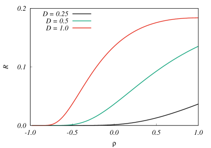
Figure 3: Rate of escape $R$ of the dimer from the potential minima to the basin of attraction of the other minima as a function of correlation $\rho$ for different values of noise intensity $D$ in the strong coupling limit between the monomers.

Fig. 3 shows the variation of the rate of escape $R$ of the dimer as a function of the noise correlation $\rho$ for different values of noise intensity $D$ when the coupling between the monomers is very strong. The monotonic variation of $R$ with $\rho$ in the strong coupling limit conforms with numerically observed results for relatively weaker values of $k$. In addition, as the probability density relaxes towards its stationary value at the same rate as the escape rate, the results in Fig. 3 also imply that the system may take a very long time to relax to its stationary state when the noise processes are strongly anticorrelated. This can leave the dimer confined in the potential minima for longer times as compared to independent noise sources and can be employed as a mechanism for confinement. With the transient properties of the dimer motion understood, in the next section let us generalize to the dynamics of a polymer in a confining potential.

IV Generalization to polymer dynamics

The dynamics of a polymer chain in some potential $U=U(x_{1},\ldots,x_{N})$ is given by the Langevin equation:

$$\dot{x}_{i}=k(x_{i-1}-2x_{i}+x_{i+1})-\frac{\partial}{\partial x_{i}}U({\bf x})+\eta_{i}(t),$$ (10)

where $i=1,\ldots,N$, and the noise processes $\eta_{i}$ are Gaussian white with mean zero and correlations $\langle\eta_{i}(t)\eta_{j}(t^{\prime})\rangle=2D\rho_{ij}\delta(t-t^{\prime})$. The diagonal elements of the correlation matrix are unity by definition and the off-diagonal elements are symmetric and take values from the interval $[-1,1]$, which generalizes the dynamics of a polymer chain with independent noise processes mesfin . The dynamical equations in (10) can be transformed to the equation for the motion of the center of mass and the motion of monomers relative to the center of mass. The equation of motion for the center of mass of the polymer:

$$\dot{x}_{c}=-\sum_{i}\frac{\partial}{\partial x_{i}}U({\bf x})+\zeta_{c}(t),$$ (11)

where $\zeta_{c}=\sum_{i}\eta_{i}/N$. The noise process $\zeta_{c}$ has mean zero and correlation $\langle\zeta_{c}(t)\zeta_{c}(t^{\prime})\rangle=\frac{2D}{N^{2}}(N+2\sum_{i<j}\rho_{ij})\delta(t-t^{\prime})$. Now, if the correlations $\rho_{ij}$ are chosen such that the term in the brackets becomes small, this can make the polymer to be trapped in a metastable state for longer times as compared to the uncorrelated noise processes. Positively correlated noise processes on the other hand aid in the escape with respect to uncorrelated noises. This can be easily understood in the limit when the coupling between the monomers is chosen to be very strong, adiabatic elimination of the relative coordinates rendering the equation of motion of center of mass: $\dot{x}_{c}=-\tilde{U}(x_{c})+\zeta_{c}(t)$, with $\tilde{U}$ being the effective potential. This is equivalent to the dynamics of a single particle in the potential $\tilde{U}$ and the thermal degrees of freedom controlled by the parameters $D$ and $\rho_{ij}$. As a result, the Kramers formula can be used to calculate the rate of escape from a potential minima: $R\approx\exp(-N\Delta\tilde{U}/D(1+2\sum_{i<j}\rho_{ij}/N))$, where $\Delta\tilde{U}$ is the height of the potential barrier. The expression generalizes the previously known results for $R$ for uncorrelated noise processes mesfin ; park ; lee ; sebastian by incorporating noise correlations. Now, for a given value of noise intensity $D$, the correlations $\rho_{ij}$ can always be chosen such that the term in the brackets: $1+2\sum_{i<j}\rho_{ij}/N$, becomes small enough to drastically reduce the magnitude of thermal fluctuations preventing the polymer to cross the barrier even when the assigned value of $D$ is strong enough to drive the barrier crossing process in the absence of noise correlations. On the other hand, if the correlations are chosen such that $\rho_{ij}>0$ for all $i,j$, then these enhance the magnitude of the thermal fluctuations thereby making the barrier crossing of the polymer more likely in comparison to the case with uncorrelated noises. This generalizes the results of the previous sections for dimers with correlated noises and has implications towards controlling the rates of chemical reactions involving polymers by varying the correlation between the noise processes.

V Conclusions

In summary, the paper discusses the dynamics of harmonically coupled Brownian particles in a symmetric, piecewise linear bistable potential under the effect of correlated noise processes. The main result of the study is that for a fixed value of noise intensity, positively correlated noise processes aid in the escape of the dimer from the metastable states whereas anticorrelated noises tend towards confinement provided the particles are not moving completely independent of each other. This result has significant implications towards the dynamics of polymers in potential fields, e.g.- the rates of chemical reactions involving polymers can be controlled by varying the noise correlations and if very strongly anti-correlated noises are used, then the polymer can be confined in metastable states for longer periods of time. Alternatively, correlated noise sources can be employed to confine polymers in a metastable state with the amounts of correlation controlling the residence times in the confinement. The observations also generalize to dynamics of extended objects in potentials with multiple minima, e.g.- transport of a dimer/ polymer in a tilted periodic potential reimann . The effects of noise correlations in such potentials would be observed in the variation of current across the potential, with the current reducing for negative correlations and enhanced for positive correlations. Such generalizations of the present results will be taken up in future works.

References

- (1) P. Hänggi, J. Stat. Phys. 42, 105 (1986).
- (2) H. A. Kramers, Physica 7, 284 (1940).
- (3) P. Hänggi, P. Talkner, and M. Borkovec, Rev. Mod. Phys. 62, 251 (1980).
- (4) M. Asfaw, Phys. Rev. E 82, 021111 (2010).
- (5) P. J. Park and W. Sung, J. Chem. Phys. 111, 5259 (1999).
- (6) S. K. Lee and W. Sung, Phys. Rev. E 63, 021115 (2001).
- (7) K. L. Sebastian and A. K. R. Paul, Phys. Rev. E 62, 927 (2000).
- (8) M. Asfaw and Y. Shiferaw, J. Chem. Phys. 136, 025101 (2012).
- (9) A. Fuliński and T. Telejko, Phys. Lett. A 152, 11 (1991).
- (10) Y. Jia and J. Li, Phys. Rev. E 53, 5764 (1996).
- (11) Y. Jia and J. Li, Phys. Rev. E 53, 5786 (1996).
- (12) D. Mei, G. Xie, L. Cao, and D. Wu, Phys. Rev. E 59, 3880 (1990).
- (13) D. Mei, G. Xie, and L. Zhang, Phys. Rev. E 68, 051102 (2003).
- (14) X. Sang, J. Xu, H. Wang, and C. Zheng, Phys. Scr. 88, 065002 (2013).
- (15) Raúl Toral and Pere Colet, Stochastic Numerical Methods: An Introduction for Students and Scientists, Wiley-VCH (2014).
- (16) M. H. Choi, R. F. Fox, and P. Jung, Phys. Rev. E 57, 6335 (1998).
- (17) H. Risken, The Fokker-Planck Equation: Methods of Solution and Applications, Springer-Verlag (1984).
- (18) H. L. Frisch, V. Privman, C. Nicolis, and G. Nicolis, J. Phys. A: Math. Gen. 23, L1147 (1990).
- (19) N. V. Agudov and A. N. Malakhov, Radiophysics and Quantum Electronics 36, 97 (1993).
- (20) P. Reimann, Phys. Rep. 361, 57 (2002).