Compton thick absorber in type 1 quasar 3C 345 revealed by Suzaku and Swift/BAT

Abstract

The archival data of 3C 345, a type 1 quasar at z = 0.5928, obtained with Suzaku and Swift/BAT are analysed. Though previous studies of this source applied only a simple broken power law model, a heavily obscuring material is found to be required by considering Akaike information criteria. The application of the numerical torus model by Murphy & Yaqoob (2009) surprisingly reveals the existence of Compton thick type 2 nucleus with the line-of-sight hydrogen column density of the torus of $N_{\textrm{H}}=10^{24.5}\ \textrm{cm}^{-2}$ and the inclination angle of $\theta_{\textrm{inc}}=90\degr$. However, this model fails to account for the Eddington ratio obtained with the optical observations by Gu et al. (2001) and Shen et al. (2011), or requires the existence of a supermassive black hole binary, which was suggested by Lobanov & Roland (2005), thus this model is likely to be inappropriate for 3C 345. A partial covering ionized absorber model which accounts for absorption in “hard excess” type 1 AGNs is also applied, and finds a Compton thick absorber with the column density of $N_{\textrm{H}}\simeq 10^{25}\ \textrm{cm}^{-2}$, the ionization parameter of $\log\xi\gtrsim 2$, and the covering fraction of $75\%\lesssim f_{c}\lesssim 85\%$. Since this model obtains a black hole mass of $\log\left(M_{\textrm{BH}}/M_{\sun}\right)=9.8$, which is consistent with the optical observation by Gu et al. (2001), this model is likely to be the best-fitting model of this source. The results suggest that 3C 345 is the most distant and most obscured hard excess AGN at this time.

1 Introduction

An active galactic nucleus (AGN) is one of the most energetic phenomena in the universe. AGNs are essentially classified into two types (type 1 and 2) based on whether or not broad lines such as H i, He i, and He ii are observed. According to unified models of AGNs (e.g., Urry & Padovani, 1995), this difference is due to the viewing angle of a dust torus, which surrounds a central supermassive black hole, accretion disc, and a region emitting broad lines (broad line region; BLR), since light from the BLR is blocked by the torus if viewed from an edge-on angle. This picture is supported by the findings of hidden polarized broad lines in the optical spectra of type 2 AGNs (e.g., Antonucci & Miller, 1985).

Studies based on population synthesis models of the cosmic X-ray background (CXB) suggest that a significant fraction of type 2 AGNs have a line-of-sight hydrogen column density of $N_{\rm H}\gtrsim 10^{24}\ \rm{cm}^{-2}$ (e.g., Gilli et al., 2007; Ueda et al., 2014), where the torus is optically thick for Compton scattering (Compton thick; CT). Numerical simulations predict that most AGNs experience such heavily obscured phase in their early stage of growth (e.g., Hopkins et al., 2005). To study these objects provides us fundamental information of the cosmic evolution of supermassive black holes and galaxies. On the other hand, recent X-ray observations find that there are CT absorbers in some type 1 AGNs (e.g., Turner et al., 2009). Hence the hydrogen column density is one of key parameters to characterize an AGN as well as the black hole mass and accretion rate. However, these sources are missed by observations below 10 keV due to the strong photoelectric absorption. Sensitive hard X-ray observations above 10 keV, where the penetrating power overwhelms the absorption, are crucial for these sources.

3C 345 ($z=0.5928$) is a type 1 quasar in the 3C catalogue (Edge et al., 1959) referred to as core-dominated radio source since its high-frequency radio emission is dominated by a compact flat spectrum (Laing et al., 1983, and references therein). It was firstly detected as a 2-keV X-ray source by Einstein (Ku et al., 1980). Neugebauer et al. (1979) found that the optical and infrared continua of the source show strong time variability on time scales of months. Moore & Stockman (1981) observed strong polarization and its large changes occurred on time scales of a week in the optical band. The apparent velocity of the jet component of the source is superluminal ($v\simeq 15c$) (Unwin et al., 1983). The supermassive black hole mass is estimated to be $\log\left(M_{\textrm{BH}}/M_{\sun}\right)=9.901$ based on the H$\beta$ line width by Gu et al. (2001, hereafter GCJ01). Similarly, Shen et al. (2011, hereafter S11) derived the black hole mass of $\log\left(M_{\textrm{BH}}/M_{\sun}\right)=9.27\pm 0.09$ and the Eddington ratio of $\log\lambda_{\textrm{Edd}}=-0.1$ based on the H$\beta$ line width and its luminosity. Recently, observations with Chandra and Hubble Space Telescope were performed (Kharb et al., 2012) to constrain the physical properties of the jet.

While 3C 345 is intensively studied for its unique natures, there is no report of the existence of a CT absorber at this time; I analysed archival data of 3C 345 obtained with Suzaku and Swift/BAT by utilizing the numerical torus model provided by Murphy & Yaqoob (2009, hereafter MY09) and photo-ionization models computed with the XSTAR code (Kallman & Bautista, 2001), and found that this source is obscured by a CT material. In this paper, I present the results of a detailed analysis of the Suzaku and Swift/BAT spectra. This paper is organized as follows. Section 2 describes the observations and data reduction. Firstly, I analyse the spectra with a conventional broken power law model in Section 3. Next, the spectra are analysed with torus absorption models in Section 4. Lastly, I present the results obtained with partial covering absorber models in Section 5. The discussion and summary follow Section 6 and 7. I adopt the cosmological parameters $(H_{0},\Omega_{\textrm{m}},\Omega_{\lambda})=(70\ \textrm{km}\ \textrm{s}^{-1}\ \textrm{Mpc}^{-1},0.3,0.7)$, the photoelectric absorption cross-sections of Verner et al. (1996) (vern in XSPEC), and the solar abundances of Anders & Grevesse (1989) (angr in XSPEC) through the paper. The errors are 90% confidence limits for a single parameter.

2 Observation and Data Reduction

2.1 Observation

Suzaku observed 3C 345 on 2012 September 11 with a net exposure of 12.7 ks. The data are public on the Suzaku page on Data ARchives and Transmission System (DARTS), and the observation ID is 707043010. Suzaku (Mitsuda et al., 2007) carries four X-ray CCD cameras called the X-ray Image Spectrometers (XIS-0, XIS-1, XIS-2, and XIS-3), which cover the 0.2–12 keV band, as the focal plane imager of four X-ray telescopes, and non-imaging instrument called the Hard X-ray Detector (HXD) consisting of Si PIN photo-diodes and Gadolinium Silicon Oxide (GSO) scintillation counters, which cover the 10–70 keV and 40–600 keV band, respectively. XIS-0, XIS-2, and XIS-3 are front-side illuminated CCDs (FI-XISs), and XIS-1 is the back-side illuminated one (BI-XIS). Since XIS-2 became inoperable on 2007 November 7 (Dotani & the XIS Team, 2007), no XIS-2 data is available. Spaced-row charge injection (SCI) was applied to the XIS data to improve the energy resolution (Nakajima et al., 2008). 3C 345 was observed at the XIS nominal position. In the spectral analysis, the 70-month (between 2004 December and 2010 September) integrated Swift/BAT spectrum covering the 15–200 keV band (Swift J1643.1+3951, Baumgartner et al., 2013) is utilized.

2.2 Data Reduction

The Suzaku data are reduced with the HEAsoft version 6.18 and the latest version of CALDB on 2016 February 24. All event files are reprocessed with the aepipeline command, and the produced cleaned events are analysed. The light curves and spectra of XISs are extracted from a circular region with a $1\arcmin.5$-radius around the detected position. The backgrounds are taken from a circular source-free region with a $3\arcmin$-radius. The so-called “tuned” non-X-ray background (NXB) model provided by the HXD team is used for the HXD/PIN data, whose systematic errors are estimated to be $\simeq 1.4\%$ at a $1\sigma$ confidence level in the 15–40 keV band for a 10 ks exposure (Fukazawa et al., 2009). The CXB spectrum simulated with the HXD/PIN response for a uniformly extended emission is added to the NXB spectrum. The HXD/GSO data are not analysable since no background model is provided.

2.3 Light Curves

Figure 1 shows the background-subtracted light curves of 3C 345 obtained with the Suzaku XIS and HXD/PIN in the 2–10 keV and 15–40 keV band, respectively. The data from XIS-0 and XIS-3 are summed. To minimize any systematic uncertainties caused by the orbital change of the satellite, the data taken during one orbit ($\simeq$ 96 minutes) are merged into one bin, and this yields 4 and 3 bins for XIS and HXD/PIN, respectively; note that the HXD/PIN observation started about 30 minutes after the XIS observation started according to the FITS headers. To check whether there are any significant time variabilities during the observation, I perform a simple $\chi^{2}$ test to each light curve, assuming a null hypothesis of constant flux. The resultant reduced $\chi^{2}$ value and the degrees of freedom are superimposed on Figure 1. Though the time variability in the XIS cannot be rejected at the 90% confidence level, the flux changes are marginal; the one in the HXD/PIN can be ruled out at the level. Thus the time-averaged spectra over the entire observation are analysed.

             

Figure 1: Background-subtracted light curves of Suzaku. One bin corresponds to 96 minutes. The numbers listed in each panel are the value of reduced $\chi^{2}$ with the degrees of freedom for the constant flux hypothesis. Left: the light curves of the XIS in the 2–10 keV band, where the data from XIS-0 and XIS-3 are summed. Right: the light curves of the HXD/PIN in the 15–40 keV band. Note that the HXD/PIN observation started about 30 minutes after the beginning of the XIS observation.

2.4 Spectra

The spectra of FI-XISs are summed; the data of the FI-XISs, BI-XIS, HXD/PIN, and Swift/BAT in the energy band of 0.8–10.0 keV, 0.5–8.0 keV, 15-25 keV, and 15–100 keV, respectively, are used, covering the 0.5–100 keV band simultaneously. The relative normalization of the PIN with respect to the FI-XISs is fixed at 1.16 based on the calibration of the Crab Nebula (Maeda et al., 2008). Those of BI-XIS and BAT with respect to the FI-XISs are set as free parameters. Galactic absorption is always included in all the models discussed in this paper; its hydrogen column density is fixed at the value calculated with the nh command, $N_{\textrm{H}}^{\textrm{Gal}}=1.14\times 10^{20}\ \textrm{cm}^{-2}$, which is based on the result of the H i map (Kalberla et al., 2005).

3 Conventional Broken Power Law Model

Table 1: Best-fitting parameters with Model A

	Energy Band	0.5–100 keV	0.5–6.0 keV	6.0–100 keV
(1)	$N_{\rm H}$ ($10^{24}\ \textrm{cm}^{-2}$)	$2.3\times 10^{-11}$ ($<4.4\times 10^{-3}$)	$2.0\times 10^{-3}$ ($<5.0\times 10^{-3}$)	$1.2\pm 0.7$
(2)	$\Gamma_{\textrm{soft}}$	$1.67\pm 0.07$	$2.3^{+0.9}_{-0.4}$	1.7a
(3)	$\Gamma_{\textrm{hard}}$	$1.1^{+0.5}_{-0.4}$	$1.7\pm 0.1$	$1.3\pm 0.4$
(4)	$E_{\textrm{break}}$ (keV)	$8^{+10}_{-6}$	$2.1^{+0.9}_{-0.4}$	$10$ ($<45$)
(5)	$A_{\textrm{BAT}}$	$0.6^{+1.0}_{-0.4}$	—	$0.40\pm 0.07$
(6)	$F_{\textrm{2-10}}$ ($10^{-12}\ \textrm{erg}\ \textrm{cm}^{-2}\ \textrm{s}^{-1}$)	2.7	2.6	1.4
(7)	$F_{\textrm{10-50}}$ ($10^{-11}\ \textrm{erg}\ \textrm{cm}^{-2}\ \textrm{s}^{-1}$)	0.98	0.45	1.7
(8)	$L_{\textrm{2-10}}$ ($10^{46}\ \textrm{erg}\ \textrm{s}^{-1}$)	0.32	0.33	0.83
(9)	$\textrm{AIC}_{c}$	$-77.42$	—	—
	$\chi^{2}/\textrm{d.o.f.}$	$111.57/177$	$90.75/158$	$6.16/12$

^aFixed.

Note. (1) The line-of-sight hydrogen column density. (2) The power law photon index below $E_{\textrm{break}}$. (3) The power law photon index above $E_{\textrm{break}}$. (4) The break energy. (5) The relative normalization of the BAT with respect to the FI-XISs. (6) The observed flux in the 2–10 keV band. (7) The observed flux in the 10–50 keV band. (8) The 2–10 keV intrinsic luminosity corrected for the absorption. (7) The corrected Akaike information criterion.

To start with, I fit the Suzaku and Swift/BAT spectra of 3C 345 with a simple broken power law model, which is represented as zphabs*zbknpower in XSPEC terminology and whose photon spectrum $F\left(E\right)$ is expressed as

$$F\left(E\right)=\begin{cases}AE^{-\Gamma_{\textrm{soft}}}&E\leq E_{\textrm{break}}\\ AE^{\Gamma_{\textrm{hard}}-\Gamma_{\textrm{soft}}}_{\textrm{break}}\left(\dfrac{E}{1\ \textrm{keV}}\right)^{-\Gamma_{\textrm{hard}}}&E>E_{\textrm{break}},\end{cases}$$ (1)

where $E$ is the photon energy in the rest frame, $E_{\textrm{break}}$ is the break energy of the power law component in the rest frame, $\Gamma_{\textrm{soft}}$ and $\Gamma_{\textrm{hard}}$ are the photon indexes for the soft and hard components, respectively, based on Gambill et al. (2003, hereafter G03) and Belsole et al. (2006, hereafter B06); the authors analysed the spectra of the core component of 3C 345 obtained with Chandra with this model. For the fitting algorithm, the standard Levenberg-Marquardt method (leven in XSPEC) is applied through this section.

Table 1 shows the best-fitting parameters obtained with Model A. B06, for example, reported flattening of the 3C 345 spectrum (the photon index of $\Gamma=1.3$) above 1.7 keV (in the observer frame) and a necessity of two power law components. However, the simultaneous fit of the XISs, HXD/PIN, Swift/BAT spectra yields a quite different break energy ($E_{\textrm{break}}=8\ \textrm{keV}$) from those of G03 and B06.

For further investigation, the spectra are divided at 6 keV, which corresponds to 9.6 keV ($\sim E_{\textrm{break}}$) in the source redshift, and fitted with Model A separately. The spectral fitting in the 0.5–6.0 keV band agrees with the results of G03 and B06 within the errors except for the photon index for the harder spectrum ($\Gamma_{\textrm{hard}}$); in the 6.0–100 keV spectra, $\Gamma_{\textrm{hard}}$ and $E_{\textrm{break}}$ agree with the literature within the errors, while the photon index for the softer spectrum is fixed at $\Gamma_{\textrm{soft}}=1.7$ due to its very weak constraint. Note that the choice of $\Gamma_{\textrm{soft}}$ does not affect the other best-fitting parameters. Interestingly, the spectra in the 6.0–100 keV band suggest that this source can be a CT-AGN. In such case, the transmitted component of the intrinsic power law through the absorber is strongly suppressed due to the strong photoelectric absorption, and the “scattered” (unabsorbed) and Compton reflection ones are only detectable below 10 keV; the transmitted component becomes comparable to the scattered one around this energy, and the spectrum seems to be flatter there. Previous studies below 10 keV could observe only the unabsorbed scattered component.

4 Torus Absorption Models

4.1 Analytic Torus Model

Since the best-fitting parameters with Model A suggest that 3C 345 can be a CT-AGN, I fit the spectra with an absorbed power law model with an exponential cutoff, an absorbed Compton reflection and its reprocessed lines from an infinitely thick reflector (Model B), which is often applied to obscured AGNs (e.g., Eguchi et al., 2009). Model B is written as zphabs*zhighect*zpowerlw + const*zhighect*zpowerlw + zphabs*pexmon in XSPEC terminology, and the photon spectrum is represented as

$$F\left(E\right)= \exp\left\{-N_{\textrm{H}}\sigma\left(E\right)\right\}I\left(E\right)$$ (2)

$$+\exp\left\{-N_{\textrm{H}}^{\textrm{refl}}\sigma\left(E\right)\right\}C\left(E\right)$$

$$+fI\left(E\right),$$

where $I\left(E\right)\equiv AE^{-\Gamma}\exp\left(-E/E_{\textrm{cut}}\right)$ is the intrinsic cutoff power law component, $\Gamma$ is the photon index, $E_{\textrm{cut}}$ is the cutoff energy of the power law component, $N_{\textrm{H}}$ is the line-of-sight hydrogen column density of absorbed component, $\sigma\left(E\right)$ is the cross-section of photoelectric absorption, $C\left(E\right)$ is the Compton reflection component (Magdziarz & Zdziarski, 1995) and its reprocessed lines (Nandra et al., 2007), $N_{\textrm{H}}^{\textrm{refl}}$ is the line-of-sight hydrogen column density of the reflection component, and $f$, which corresponds to the scattered fraction in type 2 AGNs, is the relative strength of unabsorbed component with respect to the intrinsic cutoff power law component. A restriction of $N_{\textrm{H}},N_{\textrm{H}}^{\textrm{refl}}\leq 5\times 10^{24}\ \textrm{cm}^{-2}$ is put on. The inclination angle of the reflector viewed from the nucleus is fixed at $60\degr$. I let $E_{\textrm{cut}}$ free to vary within $0\leq E_{\textrm{cut}}\leq 10^{4}\ \textrm{keV}$. The photon index, cutoff energy, and normalization of the unabsorbed and reflection components are tied to those of the absorbed component. The standard Levenberg-Marquardt method is applied here for the fitting algorithm.

Table 2: Best-fitting parameters with Model B, E₁ and E₂

	Parameter	Model B	Model E1	Model E2
(1)	$N_{\textrm{H}}$ ($10^{24}\ \textrm{cm}^{-2}$)	3.1 ($>1.2$)	3.3 ($>1.8$)	$0^{a}$
(2)	$\Gamma$	$1.68^{+0.06}_{-0.08}$	$1.69^{+0.07}_{-0.09}$	$1.69\pm 0.09$
(3)	$E_{\textrm{cut}}$ (keV)	$>129$	$>122$	$>267$
(4)	$N_{\textrm{H}}^{\textrm{refl}}$ ($10^{24}\ \textrm{cm}^{-2}$)	$=N_{\textrm{H}}$	$0^{a}$	$0^{a}$
(5)	$R$	$8.6\times 10^{-2}$ ($<2.5$)	$1.9^{+11.3}_{-1.6}\times 10^{-2}$	0.33 ($<0.81$)
(6)	$f$ or $f_{c}$ (%)	37 ($>24$)	$76^{+9}_{-11}$	$100^{a}$
(7)	$A_{\textrm{BAT}}$	$0.5^{+0.3}_{-0.1}$	$0.5^{+0.4}_{-0.2}$	$1.3^{+0.7}_{-0.4}$
(8)	$F_{\textrm{2-10}}$ ($10^{-12}\ \textrm{erg}\ \textrm{cm}^{-2}\ \textrm{s}^{-1}$)	2.9	2.9	2.7
(9)	$F_{\textrm{10-50}}$ ($10^{-11}\ \textrm{erg}\ \textrm{cm}^{-2}\ \textrm{s}^{-1}$)	1.5	1.5	0.59
(10)	$L_{\textrm{2-10}}$ ($10^{46}\ \textrm{erg}\ \textrm{s}^{-1}$)	0.85	1.3	0.30
(11)	$\textrm{AIC}_{c}$	$-85.19$	$-85.33$	$-76.50$
	$\chi^{2}/\textrm{d.o.f.}$	$105.69/176$	$105.61/176$	$113.45/178$

^aFixed.

Note. (1) The line-of-sight hydrogen column density of the absorbed power law component. (2) The power law photon index. (3) The cutoff energy of the intrinsic power law component. (4) The line-of-sight hydrogen column density of the reflection component. (5) The relative strength of the reflection component with respect to the intrinsic power law component, defined as $R\equiv\Omega/2\pi$, where $\Omega$ is the solud angle of the reflector viewed from the nucleus. (6) The relative strength of the unabsorbed (scattered) component with respect to the intrinsic power law component ($f$), or the covering fraction of the absorber ($f_{c}$). (7) The relative normalization of the BAT with respect to the FI-XISs. (8) The observed flux in the 2–10 keV band. (9) The observed flux in the 10–50 keV band. (10) The 2–10 keV intrinsic luminosity corrected for the absorption. (11) The corrected Akaike information criterion.

Table 2 represents the best-fitting parameters obtained with Model B. The hydrogen column density of the reflection component $N_{\textrm{H}}^{\textrm{refl}}$ is linked to that of the absorbed power law one $N_{\textrm{H}}$ since $N_{\textrm{H}}^{\textrm{refl}}$ exceeds $N_{\textrm{H}}$ if there is no constraint. The best-fitting value $N_{\textrm{H}}=10^{24.5}\ \textrm{cm}^{-2}$ suggests that this source is a CT-AGN. Note that only photoelectric absorption is considered, and that Compton scattering, which cannot be negligible for a CT-AGN, is not taken into account here; fully consistent treatment is given in Section 4.3. The relative strength of the Compton reflection component with respect to the intrinsic power law one $R$ is defined as $R\equiv\Omega/2\pi$, where $\Omega$ is the solid angle of the reflector, and its best-fitting value is remarkably small ($R=8.6\times 10^{-2}$) while its 90% upper limit also permits the reflection dominant case ($R<2.5$). On the other hand, the “scattered” fraction $f$ is significantly larger than those of optical selected Seyfert 2 galaxies: 3–10% (Guainazzi et al., 2005). This can reflect a contamination by the jet components in 3C 345 since this source is a radio-loud AGN.

4.2 Comparison of Model A and B

The best-fitting $\chi^{2}$ value of Model B is less than that of Model A, $\Delta\chi^{2}=-5.88$. To quantify whether this improvement is statistically significant, I introduce Akaike information criterion (AIC, Akaike, 1974). The AIC is defined as

$$\textrm{AIC}\equiv-2\ln\mathcal{L}_{\textrm{max}}+2k,$$ (3)

where $\mathcal{L}_{\textrm{max}}$ is the maximum likelihood achievable by the model, and $k$ is the number of parameters of the model. The best model minimizes the AIC. For $\chi^{2}$ minimization regime, Equation (3) is written as

$$\textrm{AIC}=N\ln\dfrac{\chi^{2}_{\textrm{min}}}{N}+2k,$$ (4)

where $N$ is the number of data points (Burnham & Anderson, 2004). Since the AIC supposes that $N$ is infinite, a correction term is required for a small sample size:

$$\textrm{AIC}_{c}=\textrm{AIC}+\dfrac{2k\left(k+1\right)}{N-k-1}$$ (5)

(Sugiura, 1978). I denote the $\textrm{AIC}_{c}$ of the $i$-th model as $\textrm{AIC}_{c,i}$, and define $\Delta_{i}$ as

$$\Delta_{i}\equiv\textrm{AIC}_{c,i}-\textrm{AIC}_{c,\textrm{min}},$$ (6)

where the subscript “min” represents the model whose $\textrm{AIC}_{c}$ is smallest of the models. An Akaike weight is defined as

$$w_{i}\equiv\dfrac{\exp\left(-\Delta_{i}/2\right)}{\displaystyle\sum_{r=1}^{R}\exp\left(-\Delta_{r}/2\right)},$$ (7)

where $R$ is the number of the models, and this can be interpreted as a model likelihood (Akaike, 1981; Burnham & Anderson, 2004)

I compute the $\textrm{AIC}_{c}$s for Model A and B, which are given in Table 1 and 2, respectively; since $\Delta_{A}=7.8$ is obtained, Model B is not “decisively” but “strongly” preferred according to Liddle (2007), and their Akaike weights ($w_{B}/w_{A}$) suggest that the odds ratio is approximately 50:1 against Model A. Hence I conclude that Model B is better than Model A.

4.3 Numerical Torus Model

             

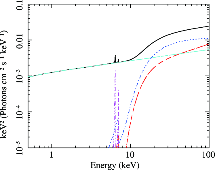
Figure 2: Observed spectra (left) and the best-fitting spectral model (right) with Model C. Left: the black crosses, red filled circles, magenta open circles, and blue crosses correspond to the data of the FI-XISs, BI-XIS, HXD/PIN, and BAT, respectively, with their $1\sigma$ error bars. The spectra of the XIS and PIN are folded with the detector response in units of $\textrm{counts}\ \textrm{s}^{-1}\ \textrm{keV}^{-1}$, while those of the BAT are corrected for the detector area and have units of $\textrm{photons}\ \textrm{cm}^{-2}\ \textrm{ks}^{-1}\ \textrm{keV}^{-1}$. The best-fitting results are plotted by solid lines, and the residuals in units of $\chi$ are shown in the lower panels. Right: the best-fitting spectral model in units of $EF_{E}$ (where $E$ is the photon energy in the rest frame and $F_{E}$ is the photon spectrum); the solid black, dashed red, dotted blue, dotted-dashed cyan, dotted-dotted-dashed magenta curves correspond to the total, absorbed transmitted component, absorbed reflected component, unabsorbed power law component, and emission lines, respectively.

Table 3: Best-fitting parameters with Model C

	Parameter	Model C
(1)	$N_{\textrm{H}}^{\textrm{Eq}}$ ($10^{24}\ \textrm{cm}^{-2}$)	$3.2\pm 0.9$
(2)	$\theta_{\textrm{inc}}$ (degree)	$88\pm 2$
(3)	$\Gamma$	$1.69\pm 0.05$
(4)	$f$ (%)	$10\pm 1$
(5)	$A_{\textrm{BAT}}$	$0.47\pm 0.08$
(6)	$F_{\textrm{2-10}}$ ($10^{-12}\ \textrm{erg}\ \textrm{cm}^{-2}\ \textrm{s}^{-1}$)	2.8
(7)	$F_{\textrm{10-50}}$ ($10^{-11}\ \textrm{erg}\ \textrm{cm}^{-2}\ \textrm{s}^{-1}$)	1.5
(8)	$L_{\textrm{2-10}}$ ($10^{46}\ \textrm{erg}\ \textrm{s}^{-1}$)	3.1
(9)	$\textrm{AIC}_{c}$	$-86.70$
	$\chi^{2}/\textrm{d.o.f.}$	$106.08/177$

(1) The hydrogen column density of the torus viewed from the equatorial direction. (2) The inclination angle of the torus. (3) The power law photon index. (4) The fraction of unabsorbed component relative to absorbed one. (5) The relative normalization of the BAT with respect to the FI-XISs. (6) The observed flux in the 2–10 keV band. (7) The observed flux in the 10–50 keV band. (8) The 2–10 keV intrinsic luminosity corrected for the absorption. (9) The corrected Akaike information criterion.

MY09 performed Monte Carlo simulations to obtain X-ray spectra from a toroidal torus with the half-opening angle of the torus of $60\degr$. The results are distributed as a set of FITS tables, and can be imported via the atable and etable models in XSPEC. I refer to the results as MYTorus model.

In MYTorus model, Thomson and relativistic Compton scattering processes are taken into account in addition to photoelectric absorption. Thus MYTorus model is much more reliable than Model B even for CT cases. MYTorus model originally consists of three components: MYTZ, MYTS, and MYTL. MYTZ is the zeroth-oder continuum, that is, absorbed transmitted power law component through the torus, MYTS is a sum of the absorbed and unabsorbed reflected continua by the torus, and MYTL represents the reprocessed emission lines by the torus. MYTS and MYTL have three parameters: the photon index $\Gamma$, the hydrogen column density of the torus viewed from the equatorial direction $N_{\textrm{H}}^{\textrm{Eq}}$, and the inclination angle of the torus $\theta_{\textrm{inc}}$ while MYTZ has two parameters: $N_{\textrm{H}}^{\textrm{Eq}}$ and $\theta_{\textrm{inc}}$.

In this subsection, I apply MYTorus model to the Suzaku and Swift/BAT spectra of 3C 345 to draw the physical property of its absorber, which is temporarily assumed to be a dust torus here. I define Model C as a sum of these three torus components together with an “scattered” unabsorbed power law component; the photon spectrum $F\left(E\right)$ of Model C can be written as

$$F\left(E\right)= \exp\left\{-\textrm{MYTZ}\left(N_{\textrm{H}}^{\textrm{Eq}},\theta_{\textrm{inc}},E\right)\right\}I^{\prime}\left(E\right)$$ (8)

$$+\textrm{MYTS}\left(N_{\textrm{H}}^{\textrm{Eq}},\theta_{\textrm{inc}},\Gamma,E\right)$$

$$+\textrm{MYTL}\left(N_{\textrm{H}}^{\textrm{Eq}},\theta_{\textrm{inc}},\Gamma,E\right)$$

$$+fI^{\prime}\left(E\right),$$

where $I^{\prime}\left(E\right)\equiv AE^{-\Gamma}$ is the intrinsic power law component, $E$ is the photon energy in the rest frame, and $f$ is the relative strength of the unabsorbed power law component with respect to the intrinsic power law one. Model C is also written as etable{mytorus_Ezero_v00.fits}*zpowerlw + atable{mytorus_scatteredH500_v00.fits} + atable{mytl_V000010nEp000H500_v00.fits} + const*zpowerlw in XSPEC terminology. For the fitting algorithm, the MINUIT MIGRAD method (migrad in XSPEC) is applied through this subsection since the standard Levenberg-Marquardt method is sometimes inappropriate for table models.

The resultant best-fitting parameters of Model C are summarized in Table 3. We find that we are seeing the absorber (torus) of this object from a completely edge-on angle ($\theta_{\textrm{inc}}\simeq 90\degr$). The hydrogen column density ($N_{\textrm{H}}^{\textrm{Eq}}=10^{24.5}\ \textrm{cm}^{-2}$) and the photon index $\Gamma$ are consistent with those obtained with Model B, suggesting that this source is a CT-AGN. On the other hand, the strength of the unabsorbed power law component relative to the intrinsic one is about one third of Model B.

The observed spectra fitted with Model C and the model spectrum are shown in Figure 2. CT-AGNs usually show a distinct Fe K$\alpha$ emission and deep Fe K edge in their X-ray spectra, but we cannot see such features in our spectra. The simple explanation for this is that the spectra below 10 keV are completely dominated by the unabsorbed power law component as can be seen from the figures, and it completely hides such spectral features.

5 Partial Covering Absorber Models

Recent studies find that in some broad line Seyfert 1 galaxies their nuclei are partially covered with CT absorbers (e.g., Turner et al., 2009). Since the line-of-sight hydrogen column density of 3C 345 is extremely high, I investigate whether partial covering absorber models can account for the spectra of 3C 345 in this section.

5.1 Cloud-Like Absorber Model

Table 4: Best-fitting parameters with Model D

	Parameter	Model D
(1)	$N_{\textrm{H}}$ ($10^{24}\ \textrm{cm}^{-2}$)	$2.4\pm 0.6$
(2)	$\Gamma$	$1.69\pm 0.05$
(3)	$f_{c}$ (%)	$94\pm 2$
(4)	$A_{\textrm{BAT}}$	$0.50\pm 0.09$
(5)	$F_{\textrm{2-10}}$ ($10^{-12}\ \textrm{erg}\ \textrm{cm}^{-2}\ \textrm{s}^{-1}$)	3.0
(6)	$F_{\textrm{10-50}}$ ($10^{-11}\ \textrm{erg}\ \textrm{cm}^{-2}\ \textrm{s}^{-1}$)	1.4
(7)	$L_{\textrm{2-10}}$ ($10^{46}\ \textrm{erg}\ \textrm{s}^{-1}$)	5.1
(8)	$\textrm{AIC}_{c}$	$-88.67$
	$\chi^{2}/\textrm{d.o.f.}$	$106.19/178$

(1) The line-of-sight hydrogen column density of the absorber. (2) The power law photon index. (3) The covering fraction of the absorber. (4) The relative normalization of the BAT with respect to the FI-XISs. (5) The observed flux in the 2–10 keV band. (6) The observed flux in the 10–50 keV band. (7) The 2–10 keV intrinsic luminosity corrected for the absorption. (8) The corrected Akaike information criterion.

I consider the case that a CT cloud, not a torus, is incidentally in our line of sight. This can be approximated by the zeroth-oder continuum represented by MYTZ in MYTorus model (Yaqoob, 2012). I define Model D as follows:

$$F\left(E\right)= f_{c}\exp\left\{-\textrm{MYTZ}\left(N_{\textrm{H}},\theta_{\textrm{inc}}=90\degr,E\right)\right\}I^{\prime}\left(E\right)$$ (9)

$$+\left(1-f_{c}\right)I^{\prime}\left(E\right),$$

where $f_{c}$ corresponds to the covering fraction of the cloud. Model D can be expressed as const*etable{mytorus_Ezero_v00.fits}*zpowerlw + const*zpowerlw in XSPEC terminology.

The best-fitting parameters of Model D are summarized in Table 4. The line-of-sight hydrogen column density is $N_{\textrm{H}}=10^{24.4}\ \textrm{cm}^{-2}$, and the covering fraction is $f_{c}\simeq 95\%$, meaning that a CT absorber covers a large solid angle of the nucleus, and it is likely to be not a cloud but a classical torus.

5.2 Compton Reflection Model

As is obvious from Figure 2, the flux above 20 keV of 3C 345 is remarkably higher than that below 20 keV. Since such spectral feature can be explained by a strong Compton reflection component, Model E₁ is defined as follows:

$$F\left(E\right)= f_{c}\exp\left\{-N_{\textrm{H}}\sigma\left(E\right)\right\}I\left(E\right)$$ (10)

$$+\exp\left\{-N_{\textrm{H}}^{\textrm{refl}}\sigma\left(E\right)\right\}C\left(E\right)$$

$$+\left(1-f_{c}\right)I\left(E\right).$$

This model is written as zpcfabs*zhighect*zpowerlw + zphabs*pexmon in the XSPEC terminology. Here $N_{\textrm{H}}^{\textrm{refl}}$ and the inclination angle of the reflector are fixed at 0 and $60\degr$, respectively. As compared to Equation (2) and (10), Model E₁ is mathematically same as Model B except for the coefficient of the unabsorbed power law component $I\left(E\right)$ ($f\rightarrow\left(1-f_{c}\right)$). Note that the reflector is assumed to be the accretion disc or clouds in the BLR in Model E₁ while it is the torus in Model B.

The best-fitting parameters are summarized in Table 2. We find the relative strength of the Compton reflection component is very weak ($R<0.13$). This means that the spectral curvature around 20 keV is explained not by the Compton reflection but by heavy absorption. However, such spectral feature should be accounted for by the reflection generally. For further investigation, the hydrogen column density of the power law component and the covering fraction of the absorber in Model E₁ are fixed at $N_{\textrm{H}}=0$ and $f_{c}=100\%$, respectively, as an extreme case (Model E₂). The best-fitting parameters are also summarized in Table 2; while a relatively strong reflection component is permitted ($R<0.81$), the resultant $\chi^{2}$ and $\textrm{AIC}_{c}$ indicate that Model E₂ is inferior to Model E₁. Hence the reflection is unlikely to be essential to account for the spectral shape of this source.

5.3 Ionized Absorber Models

Observations with hard X-ray detectors recently revealed that there is a category called “hard excess” AGNs, where the X-ray flux above 10 keV is unexpectedly stronger than that predicted from the $<10$-keV spectrum, in type 1 AGNs (e.g., Walton et al., 2010; Tatum et al., 2013). Though the physics of hard excess AGNs is not well understood at this time, their hard X-ray spectra cannot be explained by Compton reflection models like pexrav but accounted for (multi-zone) ionized absorbers possibly in the BLR. Such models are investigated in this subsection.

5.3.1 Warm Absorber Model

Table 5: Best-fitting parameters with Model F₁ and F₂

	Parameter	Model F1	Model F2
(1)	$\Gamma$	$1.69^{+0.08}_{-0.07}$	$1.8\pm 0.1$
(2)	$N_{\textrm{H}}$ ($10^{24}\ \textrm{cm}^{-2}$)	3.8 ($>2.0$)	4.4 ($>2.3$)
(3)	$f_{c}$ (%)	$76^{+8}_{-19}$	$78^{+8}_{-18}$
(4)	$\log\xi$ ($\textrm{erg}\ \textrm{cm}^{-2}\ \textrm{s}^{-1}$)	1.4 ($<2.0$)	1.3 ($<2.1$)
(5)	$T$ (K)	$1.5\times 10^{5\,a}$	$1.5\times 10^{5\,a}$
(6)	$N_{\textrm{H},2}$ ($10^{24}\ \textrm{cm}^{-2}$)	—	$0.1^{b}$
(7)	$f_{c,2}$ (%)	—	19 ($<41$)
(8)	$\log\xi_{2}$ ($\textrm{erg}\ \textrm{cm}^{-2}\ \textrm{s}^{-1}$)	—	$-1.1$ ($<1.9$)
(9)	$T_{2}$ (K)	—	$3\times 10^{4\,a}$
(10)	$A_{\textrm{BAT}}$	$0.5^{+0.4}_{-0.2}$	$0.5^{+0.4}_{-0.2}$
(11)	$F_{\textrm{2-10}}$ ($10^{-12}\ \textrm{erg}\ \textrm{cm}^{-2}\ \textrm{s}^{-1}$)	3.0	3.0
(12)	$F_{\textrm{10-50}}$ ($10^{-11}\ \textrm{erg}\ \textrm{cm}^{-2}\ \textrm{s}^{-1}$)	1.5	1.5
(13)	$L_{\textrm{2-10}}$ ($10^{46}\ \textrm{erg}\ \textrm{s}^{-1}$)	1.3	1.5
(14)	$\textrm{AIC}_{c}$	$-88.64$	$-84.22$
	$\chi^{2}/\textrm{d.o.f.}$	$104.97/177$	$103.71/174$

^aFixed.

^bThe error cannot be constrained.

(1) The power law photon index. (2) The line-of-sight hydrogen column density of the (primary) absorber. (3) The covering fraction of the (primary) absorber. (4) The ionization parameter of the (primary) absorber. (5) The temperature of the (primary) absorber. (6) The line-of-sight hydrogen column density of the secondary absorber. (7) The covering fraction of the secondary absorber. (8) The ionization parameter of the secondary absorber. (9) The temperature of the secondary absorber. (10) The relative normalization of the BAT with respect to the FI-XISs. (11) The observed flux in the 2–10 keV band. (12) The observed flux in the 10–50 keV band. (13) The 2–10 keV intrinsic luminosity corrected for the absorption. (14) The corrected Akaike information criterion.

I fit the spectra with the absori model in XSPEC (Done et al., 1992), which represents the absorption by a spherical warm ionized absorber. There are 4 parameters in the absori model: the photon index $\Gamma$, the line-of-sight hydrogen column density $N_{\textrm{H}}$, the temperature of the absorber $T$, and the ionization parameter defined by $\xi=L_{\textrm{ion}}/nr^{2}$, where $L_{\textrm{ion}}$ is the isotropic luminosity of the ionization source, and $n$ is the gas density of the absorber at a distance of $r$ from the centre. Note that the abosri model does not take Compton scattering into account. The standard Levenberg-Marquardt method is applied for the fitting algorithm here.

Firstly, I consider a one-zone absorber model (Model F₁) which is described as follows:

$$F\left(E\right)=f_{c}K\left(\Gamma,N_{\textrm{H}},\xi,T\right)I^{\prime}\left(E\right)+\left(1-f_{c}\right)I^{\prime}\left(E\right),$$ (11)

where $f_{c}$ is the covering fraction of the absorber, and $K\left(\Gamma,N_{\textrm{H}},\xi,T\right)$ corresponds to the absori model. This model can be written as const*absori*zpowerlw + const*zpowerlw in the XSPEC terminology. The temperature is fixed at $T=1.5\times 10^{5}\ \textrm{K}$ due to its very weak constraint. The best-fitting parameters are summarized in Table 5; we find that the hydrogen column density is notably high, and that the absorber is not so ionized.

Next, I assume that the absorber consists of two zones and secondary shell surrounds the primary spherical layer (Model F₂). The temperatures of the primary and secondary layers are fixed at $T=1.5\times 10^{5}\ \textrm{K}$ and $T_{2}=3\times 10^{4}\ \textrm{K}$, respectively. The photon spectrum is written as

$$F\left(E\right)= \left\{f_{c,2}K\left(\Gamma,N_{\textrm{H},2},\xi_{2},T_{2}\right)+\left(1-f_{c,2}\right)\right\}$$ (12)

$$\times\left\{f_{c}K\left(\Gamma,N_{\textrm{H}},\xi,T\right)+\left(1-f_{c}\right)\right\}I^{\prime}\left(E\right),$$

where $N_{\textrm{H}}$, $\xi$, and $f_{c}$ correspond to the line-of-sight hydrogen column density, the ionization parameter, and the covering fraction of the primary layer, respectively, and $N_{\textrm{H},2}$, $\xi_{2}$, and $f_{c,2}$ are those of the secondary layer.

The best-fitting parameters are also summarized in Table 5. As is obvious from this table, the secondary layer is physically meaningless since $N_{\textrm{H},2}\ll N_{\textrm{H}}$ and the covering fraction of it is small. This is also supported by the comparison of the $\textrm{AIC}_{c}$ values; Model F₁ is 9 times as strong as Model F₂. Hence the one-zone absorber model (Model F₁) is adequate for 3C 345.

5.3.2 Ionization and Thermal Equilibrium Model

             

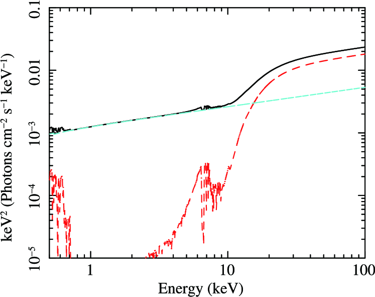
Figure 3: Observed spectra (left) and the best-fitting spectral model (right) with Model G₁₀. Left: the black crosses, red filled circles, magenta open circles, and blue crosses correspond to the data of the FI-XISs, BI-XIS, HXD/PIN, and BAT, respectively, with their $1\sigma$ error bars. The spectra of the XIS and PIN are folded with the detector response in units of $\textrm{counts}\ \textrm{s}^{-1}\ \textrm{keV}^{-1}$, while those of the BAT are corrected for the detector area and have units of $\textrm{photons}\ \textrm{cm}^{-2}\ \textrm{ks}^{-1}\ \textrm{keV}^{-1}$. The best-fitting results are plotted by solid lines, and the residuals in units of $\chi$ are shown in the lower panels. Right: the best-fitting spectral model in units of $EF_{E}$ (where $E$ is the photon energy in the rest frame and $F_{E}$ is the photon spectrum); the solid black, dashed red, and dotted-dashed cyan curves correspond to the total, absorbed transmitted component, and unabsorbed power law component, respectively.

Table 6: Best-fitting parameters with Model G₁₀, G₁₁, and G₁₂

	Parameter	Model G10	Model G11	Model G12
(1)	$n$ ($\textrm{cm}^{-3}$)	$10^{10\,a}$	$10^{11\,a}$	$10^{12\,a}$
(2)	$\Gamma$	$1.69^{a}$	$1.69^{a}$	$1.69^{a}$
(3)	$N_{\textrm{H}}$ ($10^{24}\ \textrm{cm}^{-2}$)	9.8 ($>9.2$)	10 ($>7.7$)	9.8 ($>8.5$)
(4)	$f_{c}$ (%)	$77.4\pm 0.7$	$79^{+3}_{-5}$	$78.7\pm 0.7$
(5)	$\log\xi$ ($\textrm{erg}\ \textrm{cm}^{-2}\ \textrm{s}^{-1}$)	$4\pm 1$	$1.95^{+0.14}_{-0.07}$	$2.3\pm 0.4$
(6)	$A_{\textrm{BAT}}$	$0.48\pm 0.08$	$0.46^{+0.25}_{-0.09}$	$0.46\pm 0.08$
(7)	$F_{\textrm{2-10}}$ ($10^{-12}\ \textrm{erg}\ \textrm{cm}^{-2}\ \textrm{s}^{-1}$)	2.9	2.8	2.8
(8)	$F_{\textrm{10-50}}$ ($10^{-11}\ \textrm{erg}\ \textrm{cm}^{-2}\ \textrm{s}^{-1}$)	1.5	1.6	1.6
(9)	$L_{\textrm{2-10}}$ ($10^{46}\ \textrm{erg}\ \textrm{s}^{-1}$)	1.3	1.4	1.4
(10)	$\textrm{AIC}_{c}$	$-88.30$	$-88.09$	$-88.02$
	$\chi^{2}/\textrm{d.o.f.}$	$105.16/177$	$105.28/177$	$105.32/177$

^aFixed.

(1) The gas density of the absorber. (2) The power law photon index. (3) The line-of-sight hydrogen column density of the absorber. (4) The covering fraction of the absorber. (5) The ionization parameter of the absorber. (6) The relative normalization of the BAT with respect to the FI-XISs. (7) The observed flux in the 2–10 keV band. (8) The observed flux in the 10–50 keV band. (9) The 2–10 keV intrinsic luminosity corrected for the absorption. (10) The corrected Akaile information criterion.

The limitations of the absori model are that the cross-sections above 5 keV are simply approximated by $\propto E^{-3}$, and that the absorber is in ionization equilibrium but not in thermal equilibrium. Though the spectra of 3C 345 do not show any clear line features, I solve radiative transfer by utilizing the XSTAR code to draw the more realistic nature of the absorber. The version number of the code used here is 2.39, which comes with the HEAsoft version 6.20 not with version 6.18, since some fatal bugs were fixed in the HEAsoft version 6.19 and 6.20 (see their release notes for detail). The MPI_XSTAR program is also employed for efficient usage of multi-core CPUs.

A spherical gas of uniform density is considered. The gas is assumed to be ionized by the nucleus at the centre with a single power law spectrum of a photon index of $\Gamma=1.69$. The covering fraction is fixed at 100%, and let it free to vary in XSPEC later by adding a normalization parameter $f_{c}$. The turbulence velocity of the gas is set to be $300\ \textrm{km}\ \textrm{s}^{-1}$. Iterative calculations are performed until the gas is in thermal equilibrium. The results are compiled into three table models which XSPEC can read by the xstar2table program; only a table named xout_mtable.fits, which contains the absorption spectrum in the transmitted direction, is used in this sub-subsection. When this component is expressed as $k_{n}\left(\Gamma,N_{\textrm{H}},\xi\right)$ (the subscript “$n$” represents the density of the gas), the photon spectrum of the model thought here is written as

$$F\left(E\right)=f_{c}k_{n}\left(\Gamma,N_{\textrm{H}},\xi\right)I^{\prime}\left(E\right)+\left(1-f_{c}\right)I^{\prime}\left(E\right),$$ (13)

and const*mtable{xout_mtable.fits}*zpowerlw + const*zpowerlw in the XSPEC terminology. Again, $\Gamma$ is fixed at 1.69. Note that Compton scattering is not taken into account in the XSTAR code.

The MINUIT MIGRAD method is applied here for the fitting algorithm. Three cases of gas density are computed: $n=10^{10},10^{11},10^{12}\ \textrm{cm}^{-3}$. These are referred to as Model G₁₀, G₁₁, and G₁₂, respectively. The best-fitting parameters are summarized in Table 6. Figure 3 shows the model spectrum of Model G₁₀. Overall, the ionization parameters and the line-of-sight column density of Model G_n ($n=10,11,12$) are larger than those of Model F₁. The higher a gas is ionized, the more it becomes transparent since electrons in atoms are more weakly bound and can move about freely. Thus this tendency (a higher ionization parameter leads to a higher column density) qualitatively seems correct. On the other hand, the column densities are so high that these models are not strictly accurate.

6 Discussion

6.1 Best-Fitting Models

I fitted the observed spectra of 3C 345 with 7 different models in this paper. One of them (Model A) is a simple broken power model, two of them (Model B and C) are the torus absorption models, and four of them (Model D, E_x, F_x, G_n) are the partial covering absorber models. Since Model A has no advantage over the other models due to its relatively large $\textrm{AIC}_{c}$ value, it is not discussed below.

When Model B and C are compared, while the $\textrm{AIC}_{c}$ values are comparable, Model C is physically valid even for CT cases. Thus I choose Model C as a best-fitting model. While Model D gives us the smallest $\textrm{AIC}_{c}$ of the partial covering absorber models, the result that a nearly full-coverage ($f_{c}\simeq 95\%$) absorber is in our line of sight conflicts with the assumption that the absorber is not a torus but a cloud. In Model E₁, we expect that the spectral shape can be accounted for by a strong Compton reflection component of the accretion disc or clouds in the BLR, and that the line-of-sight hydrogen column density should be rather small. However, the results lead to a very large column density of $N_{\textrm{H}}=10^{24.5}\ \textrm{cm}^{-2}$ and a very weak Compton reflection component of $R<0.13$. That is, the results conflict with the assumptions. When $N_{\textrm{H}}=0$ and $f_{c}=100\%$ are assumed (Model E₂), a rather strong reflection component is allowed ($R<0.81$). However, this model is not favoured due to the large $\textrm{AIC}_{c}$ value. Though Model F₁ reproduces the shape of the observed spectra well, there are some limitations due to the absori model. In that sense, Model G_n are more appropriate than Model F₁ since it takes radiative transfer into account and the absorber is in ionization and thermal equilibrium though Compton scattering process is not considered. Thus I also choose Model G_n as another best-fitting model.

6.2 Impact of the Uncertainty of the HXD/PIN NXB Model

As mentioned in Section 2.2, the NXB model for the HXD/PIN has systematic errors of $\simeq 1.4\%$ at a $1\sigma$ confidence level in the 15–40 keV band for a 10 ks exposure (Fukazawa et al., 2009), which is almost same as the Suzaku observation of 3C 345. To evaluate the impact of this uncertainty on my spectral fitting, I create a NXB model where count rate in each energy bin is gained 3%, conservatively, from the original “tuned” NXB model. This new NXB model is added to the CXB model spectrum used in Section 2.2, and applied to the HXD/PIN spectrum, which is simultaneously fitted with Model C together with the XIS and Swift/BAT spectra. The resultant best-fitting parameters except for the relative normalization of the Swift/BAT with respect to the FI-XISs $A_{\textrm{BAT}}$ fall within their original 90% statistical errors; $A_{\textrm{BAT}}$ changes from 0.47 to 0.55. Similarly, I also create a NXB model whose count rate is reduced by 3%, and then apply it to the observed HXD/PIN spectrum, this yielding consistent best-fitting parameters with their original values within 90% confidence limits.

Likewise, the uncertainty of the HXD/PIN NXB model is also investigated for Model G_n. The covering fraction $f_{c}$ absolutely changes by 5% ($77\%\rightarrow 82\%$, for example), and the normalization of Swift/BAT relative to the FI-XISs $A_{\textrm{BAT}}$ also changes by 0.1. The other parameters fall within the 90% confidence limits of their original values. Hence I conclude that the systematic uncertainty of the HXD/PIN NXB model does not affect our arguments.

6.3 Interpretation of the Strong Unabsorbed Component of Model C

The results fitted with Model C suggest that 3C 345 is a CT-AGN with a strong scattered (unabsorbed) component of $f=10\%$, which corresponds to the upper limit of the typical values of Seyfert 2 galaxies (3–10%, Guainazzi et al., 2005). As pointed out in Brightman et al. (2014), spectral fitting of bright unobscured sources are sometimes misidentified as CT-AGNs with a strong scattered component and a weak underlying torus component. Hence the authors introduced an upper limit of 10% of scattered component into their CT sample selection. The $f$ value of Model C falls just on this border line, and it is not rejected at this point. A possible explanation to account for the strong scattered component of this source is that the torus is more gaseous and less dusty than typical type 2 AGNs, and incident photons from the central engine are scattered in our direction by the gas by Thomson scattering. However, we have to accept the strange “facts” that 3C 345 is type 1 in the optical band but is type 2 in the X-ray band, and that the torus is viewed from a completely edge-on angle in addition.

6.4 Bolometric Luminosity and Eddington Ratio

The relative normalization of the Swift/BAT spectrum with respect to the FI-XISs is $A_{\textrm{BAT}}\simeq 0.5$ for all the models except for Model E₂, which is found to be inappropriate for 3C 345. That is, there is time variability between the Swift/BAT and Suzaku observations, and the flux observed with Suzaku is twice as high as that extrapolated from the Swift/BAT spectrum. Since the optical data are compared to the X-ray ones, this correction is always considered below.

GCJ01 derived the supermassive black hole mass of 3C 345 of $\log\left(M_{\textrm{BH}}/M_{\sun}\right)=9.901$ based on the H$\beta$ line width. S11 also derived the mass of $\log\left(M_{\textrm{BH}}/M_{\sun}\right)=9.27\pm 0.09$ and the Eddington ratio $\lambda_{\textrm{Edd},\textrm{Opt}}=0.79$ by utilizing the optical H$\beta$ line width and its luminosity in the spectrum of Sloan Digital Sky Survey (SDSS). Both authors used the same indicator but obtained different masses. This can be due to their samples. While GCJ01 focused on radio-loud quasars, S11 handled all SDSS quasars.

Firstly, I discuss the Eddington ratio $\lambda_{\textrm{Edd},\textrm{X}}$ derived from the X-ray luminosity with Model C. The absorption and time variability corrected 2–10 keV band luminosity is $L_{2-10}=1.4\times 10^{46}\ \textrm{erg}\ \textrm{s}^{-1}$. The bolometric correction for the X-ray luminosity by Marconi et al. (2004) yields a bolometric luminosity of $L_{\textrm{bol},\textrm{X}}=1.4\times 10^{48}\ \textrm{erg}\ \textrm{s}^{-1}$. Since the Eddington luminosity based on S11 is $L_{\textrm{Edd}}=2.3\times 10^{47}\ \textrm{erg}\ \textrm{s}^{-1}$, the Eddington ratio derived from the X-ray luminosity is estimated to be $\lambda_{\textrm{Edd},\textrm{X}}=5.9$ (super-Eddington), 6 times higher than that derived from the optical spectrum. When the black hole mass derived by GCJ01 is applied, the Eddington luminosity is $L_{\textrm{Edd}}=1.0\times 10^{48}\ \textrm{erg}\ \textrm{s}^{-1}$, and the Eddington ratio is $\lambda_{\textrm{Edd},\textrm{X}}=1.4$. Thus Model C is unlikely to explain the optical observations.

Next, I investigate Model G₁₀ as an example of Model G_n similarly. The 2–10 keV band luminosity is $L_{2-10}=6.4\times 10^{45}\ \textrm{erg}\ \textrm{s}^{-1}$, and the bolometric luminosity is $L_{\textrm{bol},\textrm{X}}=5.9\times 10^{47}\ \textrm{erg}\ \textrm{s}^{-1}$. The Eddington ratio based on the black hole mass by S11 is $\lambda_{\textrm{Edd},\textrm{X}}=2.5$. However, $\lambda_{\textrm{Edd},\textrm{X}}=\lambda_{\textrm{Edd},\textrm{Opt}}$ yields a black hole mass of $\log\left(M_{\textrm{BH}}/M_{\sun}\right)=9.8$, which is smaller than that by GCJ01. Thus Model G_n are likely to explain the optical spectrum. When the fact that there is no Fe K$\alpha$ line and K absorption edge in the X-ray spectrum of 3C 345 is also considered, the best-fitting model for this source is likely to be Model G_n.

6.5 Binary AGN Scenario

A calculation of the 2–10 keV band luminosity of the unabsorbed component in Model C yields $L_{2-10}=1.4\times 10^{45}\ \textrm{erg}\ \textrm{s}^{-1}$. The bolometric correction for this luminosity by Marconi et al. (2004) gives us $L_{\textrm{bol},\textrm{X}}=1.1\times 10^{47}\ \textrm{erg}\ \textrm{s}^{-1}$. When $\lambda_{\textrm{Edd},\textrm{X}}=\lambda_{\textrm{Edd},\textrm{Opt}}$ is assumed, we obtain the black hole mass of $\log\left(M_{\textrm{BH}}/M_{\sun}\right)=9.0$ or $M_{\textrm{BH}}=1.1\times 10^{9}M_{\sun}$. Interestingly, this value is slightly smaller than the lower limit of the black hole mass by S11.

Lobanov & Roland (2005) suggested that there is a supermassive black hole binary with an equal mass of $M_{\textrm{BH}}=7.1\times 10^{8}M_{\sun}$ and the separation of $\sim 0.33\ \textrm{pc}$ in 3C 345 based on the time variability in the optical and radio bands and the precession of the jet. The black hole mass obtained above is 1.5 times as heavy as that by Lobanov & Roland (2005), but their scenario seems attractive for Model C. Let us assume that both black holes have their own accretion discs and dust tori, and that one of them is a heavily absorbed CT-AGN with a type 2 nucleus with a completely edge-on viewing angle of the torus and lies behind the other one with a type 1 nucleus. An example of such systems is CID-42 (Civano et al., 2010). The X-ray spectrum of the type 2 nucleus in the 2–10 keV band is dominated by that of the type 1 nucleus due to the strong photoelectric absorption, thus the sign of the type 2 nucleus is missed in $\lesssim 10$-keV observations, but detected in $\gtrsim 10$-keV observations. This could be the case for the Suzaku and Swift/BAT spectra, and could explain the strange nature that this source is type 1 in the optical band but type 2 in the X-ray band, and the torus is viewed from a completely edge-on angle. Furthermore, if the type 2 nucleus belongs to “hidden” population (Ueda et al., 2007; Winter et al., 2009), it is hard to detect it in the optical band since the flux of the [O iii] line is too weak.

I have no evidence to prove this scenario at this time. Even if this is the case, the confirmation is very challenging even for future missions and telescopes. However, a search for an offset [O iii] line with respect to the source redshift could be worth doing.

7 Summary

The archival data of 3C 345 obtained with Suzaku and Swift/BAT are analysed. In previous studies, the X-ray spectra below 10 keV of this source were fitted with a simple broken power law model without absorption, but I found that the spectrum above 10 keV is unexpectedly stronger than that predicted by the one below 10 keV. Since such spectral shape can be explained by the strong photoelectric absorption and Compton scattering in a dense material generally, models for Compton thick AGNs and partial covering absorbers in Seyfert 1 galaxies were applied to the Suzaku and Swift/BAT spectra.

The numerical torus model by MY09, which represents the absorbed transmitted component and reflection by the torus, suggests that this source can be a Compton thick AGN with the hydrogen column density of the torus of $N_{\textrm{H}}^{\textrm{Eq}}=10^{24.5}\ \textrm{cm}^{-2}$, the inclination angle of $\theta_{\textrm{inc}}\simeq 90\degr$, and a relatively strong scattered component for typical type 2 AGNs of $f=10\%$. However, the comparison of the Eddington ratio derived from the 2–10 keV band luminosity to that of the SDSS spectrum indicates that this source is shining at a super Eddington luminosity, and this model seems inappropriate except for the possibility that 3C 345 is a binary system of supermassive black holes suggested by Lobanov & Roland (2005).

The partial covering ionized absorber model proposes that this source is a hard excess AGN with the very large absorbing column density of $N_{\textrm{H}}\simeq 10^{25}\ \textrm{cm}^{-2}$, the ionization parameter of $\log\xi\gtrsim 2\ \textrm{erg}\ \textrm{cm}^{-2}\ \textrm{s}^{-1}$, and the covering fraction of $75\%\lesssim f_{c}\lesssim 85\%$. Though the 2–10 keV band luminosity requires a relatively large black hole mass of $\log\left(M_{\textrm{BH}}/M_{\sun}\right)=9.8$, which is heavier than that estimated from the SDSS spectrum, but it is consistent with another optical observation. Thus this model is likely to the best-fitting model for 3C 345.

To my knowledge, 3C 345 is the most distant and most absorbed hard excess AGN. Further detailed observations of this source at multi-wavelengths would give us a deeper understanding of hard excess AGNs and the cosmic evolution of supermassive black holes.

References

- Akaike (1974) Akaike, H. 1974, IEEE Transactions on Automatic Control, 19, 716
- Akaike (1981) Akaike, H. 1981, Journal of Econometrics, 16, 3
- Anders & Grevesse (1989) Anders, E., & Grevesse, N. 1989, Geochimica Cosmochimica Acta, 53, 197
- Antonucci & Miller (1985) Antonucci, R. R. J., & Miller, J. S. 1985, ApJ, 297, 621
- Baumgartner et al. (2013) Baumgartner, W. H., Tueller, J., Markwardt, C. B., et al. 2013, ApJS, 207, 19
- Belsole et al. (2006) Belsole, E., Worrall, D. M., & Hardcastle, M. J. 2006, MNRAS, 366, 339
- Brightman et al. (2014) Brightman, M., Nandra, K., Salvato, M., et al. 2014, MNRAS, 443, 1999
- Burnham & Anderson (2004) Burnham, K. P., & Anderson, D. R. 2004, Sociological Methods & Research, 33, 261
- Civano et al. (2010) Civano, F., Elvis, M., Lanzuisi, G., et al. 2010, ApJ, 717, 209
- Done et al. (1992) Done, C., Mulchaey, J. S., Mushotzky, R. F., & Arnaud, K. A. 1992, ApJ, 395, 275
- Dotani & the XIS Team (2007) Dotani, T. & the XIS team 2007, JX-ISAS-SUZAKU-MEMO-2007-08, http://www.astro.isas.ac.jp/suzaku/doc/suzakumemo/suzakumemo-2007-08.pdf
- Edge et al. (1959) Edge, D. O., Shakeshaft, J. R., McAdam, W. B., Baldwin, J. E., & Archer, S. 1959, Mem. RAS, 68, 37
- Eguchi et al. (2009) Eguchi, S., Ueda, Y., Terashima, Y., Mushotzky, R., & Tueller, J. 2009, ApJ, 696, 1657
- Gambill et al. (2003) Gambill, J. K., Sambruna, R. M., Chartas, G., et al. 2003, A&A, 401, 505
- Gilli et al. (2007) Gilli, R., Comastri, A., & Hasinger, G. 2007, A&A, 463, 79
- Gu et al. (2001) Gu, M., Cao, X., & Jiang, D. R. 2001, MNRAS, 327, 1111
- Guainazzi et al. (2005) Guainazzi, M., Matt, G., & Perola, G. C. 2005, A&A, 444, 119
- Hopkins et al. (2005) Hopkins, P. F., Hernquist, L., Cox, T. J., Di Matteo, T., Martini, P., Robertson, B., & Springel, V. 2005, ApJ, 630, 705
- Kalberla et al. (2005) Kalberla, P. M. W., Burton, W. B., Hartmann, D., Arnal, E. M., Bajaja, E., Morras, R., Pöppel, W. G. L. 2005, A&A, 440, 775
- Kallman & Bautista (2001) Kallman, T., & Bautista, M. 2001, ApJS, 133, 221
- Kharb et al. (2012) Kharb, P., Lister, M. L., Marshall, H. L., & Hogan, B. S. 2012, ApJ, 748, 81
- Ku et al. (1980) Ku, W. H.-M., Helfand, D. J., & Lucy, L. B. 1980, Nature, 288, 323
- Laing et al. (1983) Laing, R. A., Riley, J. M., & Longair, M. S. 1983, MNRAS, 204, 151
- Liddle (2007) Liddle, A. R. 2007, MNRAS, 377, L74
- Lobanov & Roland (2005) Lobanov, A. P., & Roland, J. 2005, A&A, 431, 831
- Marconi et al. (2004) Marconi, A., Risaliti, G., Gilli, R., et al. 2004, MNRAS, 351, 169
- Maeda et al. (2008) Maeda, Y., Someya, K., Ishida, M., & the XRT team, Hayashida, K., Mori, H., & the XIS team 2008, JX-ISAS-SUZAKU-MEMO-2008-06, http://www.astro.isas.ac.jp/suzaku/doc/suzakumemo/suzakumemo-2008-06.pdf
- Magdziarz & Zdziarski (1995) Magdziarz, P., & Zdziarski, A. A. 1995, MNRAS, 273, 837
- Mitsuda et al. (2007) Mitsuda, K., et al. 2007, PASJ, 59, 1
- Fukazawa et al. (2009) Fukazawa, Y., Mizuno, T., Watanabe, S., et al. 2009, PASJ, 61, S17
- Moore & Stockman (1981) Moore, R. L., & Stockman, H. S. 1981, ApJ, 243, 60
- Murphy & Yaqoob (2009) Murphy, K. D., & Yaqoob, T. 2009, MNRAS, 397, 1549
- Nakajima et al. (2008) Nakajima, H., et al. 2008, PASJ, 60, 1
- Nandra et al. (2007) Nandra, K., O’Neill, P. M., George, I. M., & Reeves, J. N. 2007, MNRAS, 382, 194
- Neugebauer et al. (1979) Neugebauer, G., Oke, J. B., Becklin, E. E., & Matthews, K. 1979, ApJ, 230, 79
- Shen et al. (2011) Shen, Y., Richards, G. T., Strauss, M. A., et al. 2011, ApJS, 194, 45
- Sugiura (1978) Sugiura, N. 1978, Communications in Statistics—Theory and Methods, A7, 13
- Tatum et al. (2013) Tatum, M. M., Turner, T. J., Miller, L., & Reeves, J. N. 2013, ApJ, 762, 80
- Turner et al. (2009) Turner, T. J., Miller, L., Kraemer, S. B., Reeves, J. N., & Pounds, K. A. 2009, ApJ, 698, 99
- Ueda et al. (2007) Ueda, Y., Eguchi, S., Terashima, Y., et al. 2007, ApJ, 664, L79
- Ueda et al. (2014) Ueda, Y., Akiyama, M., Hasinger, G., Miyaji, T., & Watson, M. G. 2014, ApJ, 786, 104
- Unwin et al. (1983) Unwin, S. C., Cohen, M. H., Pearson, T. J., et al. 1983, ApJ, 271, 536
- Urry & Padovani (1995) Urry, C. M., & Padovani, P. 1995, PASP, 107, 803
- Verner et al. (1996) Verner, D. A., Ferland, G. J., Korista, K. T., & Yakovlev, D. G. 1996, ApJ, 465, 487
- Walton et al. (2010) Walton, D. J., Reis, R. C., & Fabian, A. C. 2010, MNRAS, 408, 601
- Winter et al. (2009) Winter, L. M., Mushotzky, R. F., Reynolds, C. S., & Tueller, J. 2009, ApJ, 690, 1322
- Yaqoob (2012) Yaqoob, T. 2012, MNRAS, 423, 3360