ZU-TH 04/17

Azimuthal asymmetries in QCD hard scattering:
infrared safe but divergent

Stefano Catani${}^{(a)},$ Massimiliano Grazzini^(b) and Hayk Sargsyan^(b)

^(a) INFN, Sezione di Firenze and Dipartimento di Fisica e Astronomia,

Università di Firenze, I-50019 Sesto Fiorentino, Florence, Italy

^(b) Physik-Institut, Universität Zürich, CH-8057 Zürich, Switzerland

Abstract

We consider high-mass systems of two or more particles that are produced by QCD hard scattering in hadronic collisions. We examine the azimuthal correlations between the system and one of its particles. We point out that the perturbative QCD computation of such azimuthal correlations and asymmetries can lead to divergent results at fixed perturbative orders. The fixed-order divergences affect basic (and infrared safe) quantities such as the total cross section at fixed (and arbitrary) values of the azimuthal-correlation angle $\varphi$. Examples of processes with fixed-order divergences are heavy-quark pair production, associated production of vector bosons and jets, dijet and diboson production. A noticeable exception is the production of high-mass lepton pairs through the Drell–Yan mechanism of quark-antiquark annihilation. However, even in the Drell–Yan process, fixed-order divergences arise in the computation of QED radiative corrections. We specify general conditions that produce the divergences by discussing their physical origin in fixed-order computations. We show lowest-order illustrative results for $\cos(n\varphi)$ asymmetries (with $n=1,2,4,6$) in top-quark pair production and associated production of a vector boson and a jet at the LHC. The divergences are removed by a proper all-order resummation procedure of the perturbative contributions. Resummation leads to azimuthal asymmetries that are finite and computable. We present first quantitative results of such a resummed computation for the $\cos(2\varphi)$ asymmetry in top-quark pair production at the LHC.

March 2017

1 Introduction

Angular distributions of final-state particles produced by high-energy collisions are known to be relevant observables for the understanding of the underlying dynamics of their production mechanism. In this paper we deal with azimuthal-angle distributions and related asymmetries.

In the case of collisions that are produced by spin polarized particles, azimuthal angles with respect to the spin direction can be specified and measured: the analysis of the ensuing azimuthal correlations is a much studied topic and the subject of intense ongoing investigations (see, e.g., Ref. [1] and references therein).

Azimuthal correlations in spin unpolarized collisions are less studied. A relevant exception is the lepton azimuthal distribution [2] of high invariant mass lepton pairs that are produced in hadron collisions through the Drell–Yan (DY) mechanism of quark-antiquark annihilation. Angular distributions for the DY process are a well known topic that has been deeply studied at both the theoretical and experimental levels (see, e.g., Refs. [3, 4, 5] and references therein).

In the case of spin unpolarized collisions, much attention to azimuthal asymmetries has been devoted in recent years within the context of a QCD framework based on the introduction of non-perturbative transverse-momentum dependent (TMD) distributions of quarks and gluons inside the colliding unpolarized hadrons. In particular, the TMD distribution of linearly-polarized gluons [6] inside unpolarized hadrons plays a distinctive role since it leads to specific $\cos(2\varphi)$ and $\cos(4\varphi)$ modulations of the dependence on the azimuthal-correlation angle $\varphi$. TMD distribution studies of such modulations have been performed, for instance, for the production process of heavy quark-antiquark ($Q{\bar{Q}}$) pairs [7] and for the associated production of a virtual photon and a jet ($\gamma^{*}+1$ jet) [8]. Many more related studies can be found in the list of references of Ref. [8].

In this paper we consider spin unpolarized collisions and, specifically, we focus our discussion on hadron–hadron collisions, although many features that we discuss are generalizable to (and, hence, valid for) lepton–hadron and lepton–lepton collisions. We consider the production of a system $F$ of two or more particles with a high value of the total invariant mass, and we examine the azimuthal correlations between the momenta of the system and of one of its particles. Roughly speaking, the relevant azimuthal angle $\varphi$ is related to the difference between the azimuthal angles of the transverse momenta $q_{T}$ of the system and $p_{T}$ of the particle. Considering high values of the invariant mass $M$ of the system $F$ (additional kinematical cuts on the momentum of the produced particle can be applied or required), we select the hard-scattering regime of the production process. In this regime, azimuthal correlations are infrared and collinear safe observables [9], and they can be studied and computed by applying the standard QCD framework of factorization in terms of perturbative partonic cross sections and parton distribution functions (PDFs) of the colliding hadrons. Starting from the results in Refs. [10, 11] and, especially, from those in Ref. [12] and the analysis on the role of soft wide-angle radiation that is performed therein, we develop and present some general (process-independent) considerations on azimuthal correlations and asymmetries.

We point out with some generality that, in spite of the infrared and collinear safety of azimuthal-correlation observables, their computation at fixed perturbative orders leads to divergences. The divergences appear also in basic quantities such as the total cross section at fixed (and arbitrary) values of the azimuthal-correlation angle $\varphi$. Example of processes with fixed order (f.o.) divergences are heavy-quark pair ($Q{\bar{Q}}$) production, associated production of vector ($V$) or Higgs bosons and jets (e.g., ‘$V+1$ jet’ with $V=Z,W^{\pm},\gamma^{*}$), dijet and diboson production. We support our theoretical discussion by performing the numerical calculation of $\cos(n\varphi)$ modulations (for some values of $n$) at the lowest perturbative order for some specific processes. The numerical results are found to be consistent with the divergent behaviour if $n=2,4,6$ in the case of top-quark pair ($t{\bar{t}}$) production and if $n=1,2,4,6$ in the case of associated ‘$Z+1$ jet’ production. A noticeable exception to the appearance of QCD divergences is the case of the DY process. However, even in the case of the DY process, we predict the presence of f.o. divergences in the perturbative computation of QED radiative corrections. Moreover, analogous divergences arise in the case of lepton–lepton collisions from the computation of radiative corrections in a pure QED context (e.g., in the QED inclusive-production process $e^{+}e^{-}\rightarrow\mu^{+}\mu^{-}+X$, or even in the simpler process $\gamma\gamma\rightarrow\mu^{+}\mu^{-}+X$). In summary, processes that at the leading order (LO) are produced with an exactly vanishing value, $q_{T}=0$, of the transverse momentum $q_{T}$ of the system $F$ tend to develop sooner or later (in the computation of QCD and QED radiative corrections at subsequent perturbative orders) f.o. divergences.

A possible reaction to this state of affairs is to advocate non-perturbative strong-interactions dynamics and related non-perturbative QCD effects that can cure the f.o. divergences. This cure would spoil the common wisdom according to which non-perturbative contributions to infrared and collinear safe observables are (expected to be) power suppressed, namely, suppressed by some inverse power of the relevant hard-scattering scale (as set by the high invariant mass $M$ of the system $F$). Moreover, non-perturbative strong-interactions dynamics cannot be advocated in the case of f.o. divergences in a pure QED context.

We pursue a more conventional viewpoint within perturbation theory. We examine the origin of the singularities for azimuthal-correlation observables order by order in perturbation theory, and we proceed to resum the singular terms to all orders [11, 12].

The singularities originate from the kinematical region where $q_{T}\rightarrow 0$. We identify two sources of singularities. One source [10, 11] is initial-state collinear radiation in the case of systems $F$ that can be produced with vanishing $q_{T}$ by gluon initiated partonic collisions. The other source [12] is soft wide-angle radiation in the case of systems $F$ that contain colour-charged particles (or electrically-charged particles for QED radiative corrections). Collinear radiation is, per se, responsible for singularities in $\cos(n\varphi)$ (and $\sin(n\varphi)$) harmonics with $n=2$ and $n=4$, only [11]. Soft radiation is responsible for singularities that, in principle, can affect harmonics with any (both even and odd) values of $n$ ($n=1,2,3,4\dots$).

At high perturbative orders collinear and soft radiation is mixed up, and the singularities are enhanced by logarithmic ($\ln(M/q_{T})$) contributions. We discuss in general terms how the all-order resummation of the logarithmic contributions leads to ($q_{T}$ integrated) azimuthal asymmetries that are finite and computable. Such procedure is effective in both QCD and QED contexts. In the QCD case this does not imply that non-perturbative effects have a negligible quantitative role in the region of very-low values of $q_{T}$, but these effects give small contributions to $q_{T}$-integrated azimuthal-correlation observables. Within perturbative QCD, the most advanced theoretical treatment of singular azimuthal correlations that is available at present regards the process of heavy-quark pair production [12]. We use the process of top-quark pair production in $pp$ collisions at the LHC as a prototype to present a first illustration of the resummation of singular azimuthal asymmetries at the quantitative level.

A correspondence can be established [10, 11, 13] between the TMD distribution of linearly-polarized gluons and singular azimuthal correlations that are due to initial-state collinear radiation in gluon initiated partonic subprocesses. Therefore, both the framework used in Refs. [7, 8] and our perturbative QCD treatment lead to corresponding $\cos(2\varphi)$ and $\cos(4\varphi)$ azimuthal modulations. In this respect, the TMD distribution of linearly-polarized gluons can be regarded as the extension of specific features of QCD collinear dynamics from perturbative to non-perturbative transverse-momentum scales. Much discussion of the present paper is related to soft radiation effects that occur in processes with colour-charged final-state particles. Soft radiation produces azimuthal asymmetries (which are singular at f.o. and finite after resummation) for both quark (or antiquark) and gluon initiated subprocesses, and for $\cos(n\varphi)$ harmonics with arbitrary even values ($n=2,4,6,\dots$) [12] and also odd values of $n$. These soft wide-angle radiation effects are unrelated to the TMD distribution of linearly-polarized gluons.

The paper is organized as follows. In Sect. 2 we start our discussion on azimuthal asymmetries and we specify the conditions that lead to divergences in f.o. computations. In Sect. 3 we discuss azimuthal asymmetries in two examples of hadron collider processes, i.e. the production of lepton pairs through the DY mechanism and the production of a $t{\bar{t}}$ pair, by contrasting the different behaviour of the corresponding azimuthal harmonics. In Sect. 4 we start our analysis of the small-$q_{T}$ limit: in Sect. 4.1 we focus on the small-$q_{T}$ behavior at f.o. and in Sect. 4.2 we recall the transverse-momentum resummation procedure for the case of azimuthally-averaged cross sections. In Sect. 5.1 we discuss the origin of singular azimuthal correlations and present illustrative lowest-order results for the $Z+$jet production process. In Sect. 5.2 we outline the resummation procedure of singular terms in the case of azimuthally-correlated cross sections and we contrast the small-$q_{T}$ behavior expected for the resummed cross section with the known behavior of the azimuthally-averaged transverse-momentum cross section. In Sect. 5.3 we focus on the $n=2$ harmonic for $t{\bar{t}}$ production and we present first quantitative results of a resummed calculation at next-to-leading logarithmic accuracy. After the matching with the complete next-to-leading order (NLO) result, the resummed computation offers an effective ‘lowest-order’ prediction for the $n=2$ harmonic. We also comment on the possible role of non-singular terms. In Sect. 6 we summarize our results.

2 Azimuthal correlations and asymmetries in fixed-order perturbation theory

Our discussion on azimuthal correlations has a high generality. To simplify the illustration of the key points, we consider the simplest class of processes, in which the produced high-mass system in the final state is formed by only two ‘particles’ in generalized sense (point-like particles and/or jets).

We consider the inclusive hard-scattering hadroproduction process

$$h_{1}(P_{1})+h_{2}(P_{2})\rightarrow F(\{p_{3},p_{4}\})+X\;\;,$$ (1)

in which the collision of the two hadrons $h_{1}$ and $h_{2}$ with momenta $P_{1}$ and $P_{2}$ produces the triggered final state $F$, and $X$ denotes the accompanying final-state radiation. The observed final state $F$ is a generic system that is formed by two ‘particles’, $f_{3}$ and $f_{4}$, with four momenta $p_{3}$ and $p_{4}$, respectively. The two particles can be point-like particles or hadronic jets ($j$), which are reconstructed by a suitable (infrared and collinear safe) jet algorithm. As for the case of point-like particles, the most topical process is the production of a high-mass lepton pair $\ell\ell^{\prime}$ through the DY mechanism of quark–antiquark annihilation. We consider many other cases such as, for instance, the production of a photon pair ($\gamma\gamma$), a pair of top quark and antiquark ($t{\bar{t}}$) or a pair of vector bosons ($VV$), in addition to dijet production ($jj$) and associated production processes such as vector boson plus jet ($Vj$). The invariant masses of the two particles have a little role in the context of our discussion (and they do not affect any conceptual aspects of our discussion). The system $F$ has total invariant mass $M$ ($M^{2}=(p_{3}+p_{4})^{2}$), transverse momentum $q_{T}$ and rapidity $y$ (transverse momenta and rapidities are defined in the centre–of–mass frame of the colliding hadrons). We require that $M$ is large ($M\gg\Lambda_{QCD}$, $\Lambda_{QCD}$ being the QCD scale), so that the process in Eq. (1) can be treated within the customary perturbative QCD framework. We use ${\sqrt{s}}$ to denote the centre–of–mass energy of the colliding hadrons, which are treated in the massless approximation ($s=(P_{1}+P_{2})^{2}=2P_{1}\cdot P_{2}$).

The dynamics of the production process in Eq. (1) can be described in terms of five kinematical variables: the total mass $M$, transverse momentum $q_{T}$ and rapidity $y$ of the system $F$ and two independent angular variables that specify the kinematics of the two particles $f_{3}$ and $f_{4}$ with respect to the total momentum $q=p_{3}+p_{4}$ of $F$. These two angular variables are a polar-angle variable and an azimuthal-angle variable. To be definite and to avoid the use of ‘exotic’ variables, we refer to a widely-used set of angular variables and we use the polar angle $\theta$ and the azimuthal angle $\varphi$ (of particle $f_{3}$) in the Collins–Soper (CS) rest frame [2] of the system $F$.

The variable $\varphi$ is the relevant variable for our discussion of azimuthal correlations. We remark that $\varphi$ specifies the azimuth of one of the two particles in the system $F$ with respect to the total momentum of the system. In particular, we also remark that we are not considering the relative azimuthal separation $\Delta\phi=\phi_{3}-\phi_{4}$ ($\phi_{i}=\phi({\mbox{\boldmath$p_{T}$}}_{i})$, with $i=3,4$, is the azimuthal angle of the transverse-momentum vector ${\mbox{\boldmath$p_{T}$}}_{i}$ in the centre–of–mass frame of the colliding hadrons) between the two particles. However, we can anticipate (we postpone comments on this point) that our main findings are not specific of the CS frame, and they are equally valid for other azimuthal variables with respect to the system $F$ (for instance, we can consider the azimuthal angle in a different rest frame of $F$ or, simply, the azimuthal difference $\phi({\mbox{\boldmath$p_{T}$}}_{i})-\phi({\mbox{\boldmath$q_{T}$}})$, where $\phi({\mbox{\boldmath$q_{T}$}})$ is the azimuthal angle of $q_{T}$ in the centre–of–mass frame of the colliding hadrons).

Using the kinematical variables in the CS frame, we can consider azimuthal distributions for the process in Eq. (1). The most elementary azimuthal-dependent observable is the azimuthal cross section at fixed invariant mass,

$$\frac{d\sigma}{dM^{2}\,d\varphi}\;\;,$$ (2)

and we can also consider less inclusive observables such as, for instance, the $q_{T}$-dependent azimuthal cross section in Eq. (3) and the multidifferential (five-fold) cross section in Eq. (4):

$$\frac{d\sigma}{dM^{2}\,dq_{T}^{2}\,d\varphi}\;\;,$$ (3)

$$\frac{d\sigma}{dM^{2}\,dy\,dq_{T}^{2}\,d\!\cos\theta\,d\varphi}\;\;.$$ (4)

All these quantities are related (from the less inclusive to the more inclusive case) through integration of kinematical variables (for instance, the azimuthal cross section in Eq. (2) is obtained by integrating Eq. (3) over $q_{T}^{2}$) and, in particular, the azimuthal integration of Eq. (2) gives the total cross section (at fixed invariant mass) of the process:

$$\frac{d\sigma}{dM^{2}}=\int_{0}^{2\pi}d\varphi\;\,\frac{d\sigma}{dM^{2}\,d\varphi}\;\;.$$ (5)

Obviously, we can also consider differential cross sections that are integrated over a certain range of values of the invariant mass.

Since all the cross sections that we have just mentioned are infrared and collinear safe quantities [9], they can be computed perturbatively within the customary QCD factorization framework (see Ref. [14] and references therein). The only non-perturbative (strictly speaking) input is the set of PDFs of the colliding hadrons. The PDFs are convoluted with corresponding partonic differential cross sections $d{\hat{\sigma}}$ that can be evaluated as a power series expansion in the QCD running coupling $\alpha_{\mathrm{S}}(M)$.

This perturbative QCD framework is applicable at any finite (and arbitrary) fixed perturbative order. Despite this statement, the first main observation that we want to make is that the f.o. perturbative calculation of the azimuthal distributions can lead to divergent (and, hence, unphysical and useless) results. More specifically, the f.o. calculation of the azimuthal cross section of Eq. (2) gives the following results:

$$\frac{d\sigma}{dM^{2}\,d\varphi}=\begin{cases}\text{finite at any f.o. \;\;\;\;\;\quad\quad\quad\quad\quad\quad(DY production)}\\ {}\\ \text{divergent for any $\varphi$ at some f.o. \;\;($t{\bar{t}},Vj,jj,\gamma\gamma,ZZ,W^{+}W^{-},..,$ production) }\end{cases}\;.$$ (6)

We mean that the perturbative computation of $d\sigma/dM^{2}\,d\varphi$ for the DY process gives a finite result order–by–order in QCD perturbation theory, while in most of the other cases (some of them are listed in the right-hand side of Eq. (6)) the computation gives a divergent (meaningless) result for any values of the azimuthal angle $\varphi$ starting from some perturbative order. We note that the integration over $\varphi$ of $d\sigma/dM^{2}\,d\varphi$ gives the total cross section (see Eq. (5)), which is known to be finite at any f.o.. Therefore, the divergent behaviour that is highlighted in Eq. (6) originates from the azimuthal-correlation component, $d\sigma^{\rm corr}/dM^{2}\,d\varphi$, of the azimuthal cross section:

$$\frac{d\sigma^{\rm corr}}{dM^{2}\,d\varphi}\equiv\frac{d\sigma}{dM^{2}\,d\varphi}-\langle\frac{d\sigma}{dM^{2}\,d\varphi}\rangle_{\rm av.}=\frac{d\sigma}{dM^{2}\,d\varphi}-\frac{1}{2\pi}\;\frac{d\sigma}{dM^{2}}\;\;,$$ (7)

where the notation $\langle\cdots\rangle_{\rm av.}$ denotes the azimuthal average and $d\sigma/dM^{2}$ is the total cross section in Eq. (5).

To understand the origin of the divergent behaviour in Eq. (6), we first comment about kinematics. If the system $F$ has vanishing transverse momentum ($q_{T}=0$), the rest frame of $F$ is obtained by simply applying a longitudinal boost to the centre–of–mass frame of the colliding hadrons. Any additional rotation in the transverse plane of the collision leaves the system $F$ at rest and makes the particle azimuthal angle $\varphi$ ambiguously defined. Owing to the azimuthal symmetry of the collision process, if $q_{T}=0$ there is no preferred direction to define $\varphi$. In other words, considering the azimuthal angle $\varphi$ (as defined in the CS frame or any other rest frame of $F$) and performing the limit $q_{T}\rightarrow 0$, we have

$$\cos\varphi=\cos(\phi_{3}-\phi({\mbox{\boldmath$q_{T}$}}))+{\cal O}(q_{T}/M)\;\;,$$ (8)

where $\phi_{3}=\phi({\mbox{\boldmath$p_{T}$}}_{3})$ and $\phi({\mbox{\boldmath$q_{T}$}})$ are the azimuthal angles of the corresponding transverse-momentum vectors in the centre–of–mass frame of the colliding hadrons. If $q_{T}=0$, $\phi({\mbox{\boldmath$q_{T}$}})$ is not defined and, consequently, $\varphi$ is not (unambiguously) defined. At the strictly formal level, to define the azimuthal correlation we have to exclude the phase space point at $q_{T}=0$. If we want to consider $q_{T}$ integrated azimuthal correlations (such as, for instance, the cross section in Eq. (7)), we have to introduce a minimum value of $q_{T}$ ($q_{T}>q_{\rm cut}$) and eventually perform the limit $q_{\rm cut}\rightarrow 0$. The divergences that are highlighted in Eq. (6) do not appear by considering azimuthal correlations at fixed and finite values of $q_{T}$ (e.g., the azimuthal-dependent cross sections in Eq. (3) and (4)). These divergences are related to the limit $q_{\rm cut}\rightarrow 0$ after integration of the azimuthal correlations over $q_{T}$.

Our discussion on the limit $q_{\rm cut}\rightarrow 0$ reconciles the appearance of divergences in Eq. (6) with the perturbative criterion of infrared and collinear safety at the formal level: no divergence occurs provided $q_{T}\neq 0$, namely, provided the azimuthal-correlation observable is well (unambiguously) defined. However, a single phase space point at $q_{T}=0$ is physically harmless. Therefore, the $q_{T}$ integrated azimuthal correlations (i.e., their limiting behaviour as $q_{\rm cut}\rightarrow 0$) are finite and measurable quantities. Moreover, they are also finite and measurable if $q_{\rm cut}$ is non-vanishing, or, equivalently if $q_{T}$ is not vanishing and fixed at an arbitrarily small value. The divergence in Eq. (6) implies that the $q_{T}$ dependent azimuthal correlations become singular at small values of $q_{T}$, and that this singular behaviour is not integrable over $q_{T}$ in the limit $q_{T}\rightarrow 0$. This unphysical behaviour of f.o. perturbative QCD at small values of $q_{T}$ and the divergence of the $q_{T}$ integrated azimuthal correlations certainly require some deeper understanding to have a QCD theory of physically measurable azimuthal correlations. As a possible shortcut, one can still use f.o. perturbative QCD but avoid the region of small values of $q_{T}$. In this case one still needs some understanding of the phenomenon in order to assess the extent of the dangerous small-$q_{T}$ region where the f.o. predictions are ‘unphysical’ or, anyhow, not reliable at the quantitative level.

We note that the kinematical relation in Eq. (8) implies that the azimuthal angle in the CS frame has no privileged role in the context of our discussion of azimuthal correlations in the small-$q_{T}$ region. The main features of the small-$q_{T}$ behaviour of azimuthal correlations that are discussed in this paper are basically unaffected by using azimuthal angles as defined in other rest frames of the system $F$, or, by using other related definitions of azimuthal angles. For instance, one can simply replace the CS frame angle $\varphi$ with one of the relative azimuthal angles $\phi({\mbox{\boldmath$p_{T}$}}_{i})-\phi({\mbox{\boldmath$q_{T}$}})$ ($i=3,4$) in the centre–of–mass frame of the colliding hadrons. Alternatively, one can use the difference between the azimuthal angles (in the centre–of–mass frame of the colliding hadrons) of the two transverse-momentum vectors ${\mbox{\boldmath$p_{T}$}}_{3}-{\mbox{\boldmath$p_{T}$}}_{4}$ and $q_{T}$. All these definitions of the relevant (for our purposes) azimuthal-angle variable turn out to be equivalent (because of Eq. (8)) in the limit $q_{T}\rightarrow 0$ (or, at very small values of $q_{\rm cut}$). In the following we continue to mainly refer ourselves to the azimuthal angle in the CS frame, although all the basic features that we discuss are unchanged by considering the other definitions of the azimuthal angle.

We also note that the discussion that we have presented so far about azimuthal correlations can be generalized in a straightforward way to consider the case in which the system $F$ is formed by more than two particles. In the multiparticle case, we can simply examine azimuthal correlations that are defined by using the azimuthal angles of the various particles in $F$ in a specified rest frame of $F$ (such as the CS frame), by simply using the various relative azimuthal angles $\phi({\mbox{\boldmath$p_{T}$}}_{i})-\phi({\mbox{\boldmath$q_{T}$}})$ in the centre–of–mass frame of the colliding hadrons, or by using some other related (i.e., equivalent in the limit $q_{T}\rightarrow 0$) azimuthal variables. Since the multiparticle cases do not present any additional conceptual issues with respect to the two-particle case, in the following (for the sake of technical simplicity) we continue to mostly consider the case of systems $F$ that are formed by two particles.

The f.o. perturbative divergences of the azimuthal correlations originate from QCD radiative corrections due to inclusive emission in the final state of partons with low transverse momentum (soft and collinear partons). The origin is discussed in more detail in the following Sections of the paper (see, in particular, Sect. 5.1). Since the azimuthal correlations behave differently in different processes (as stated in Eq. (6)), we anticipate here the conditions that produce the divergent behaviour.

Azimuthal correlations can have f.o. divergences if the final-state system $F(\{p_{3},p_{4}\})$ can be produced by the partonic subprocess $c_{1}\,c_{2}\rightarrow F$ (see also Eq. (15) and accompanying comments) where

$$\bullet~{}~{}{\rm at~{}least~{}one~{}of~{}the~{}initial\!-\!state~{}colliding~{}partons}\;c_{1}\;{\rm and}\;c_{2}\;{\rm is~{}a~{}gluon};$$ (9)

$$\bullet~{}~{}{\rm at~{}least~{}one~{}of~{}the~{}final\!-\!state~{}particles~{}with~{}momenta}\,p_{3}\;{\rm and}\,p_{4}\;{\rm carries~{}colour~{}charge}.$$ (10)

The conditions in (9) and (10) follow from a generalization of the results in Refs. [11, 12]. The divergences arise from the computation of the QCD radiative correction to the partonic process $c_{1}\,c_{2}\rightarrow F$ (they do not arise in the computation of that partonic subprocess itself!). Specifically, the f.o. divergences originate from collinear-parton radiation [11] in the case of the condition (9) and from soft-parton radiation [12] in the case of the condition (10). We remark that one of the conditions in (9) and (10) is sufficient to produce the f.o. divergences. In particular, the condition (10) necessarily produces f.o. divergences, while the condition (9) produces divergences with some ‘exception’ (words of caution) in few specific cases (see below). Having discussed the source of f.o. divergences in general terms, we can comment on some specific processes.

The production of heavy-quark pairs such as, for instance, $t{\bar{t}}$ can occur through the partonic subprocesses of quark-antiquark annihilation ($q{\bar{q}}\rightarrow t{\bar{t}}$) and gluon fusion ($gg\rightarrow t{\bar{t}}$). One of these subprocesses has initial-state gluons and, moreover, both $t$ and $\bar{t}$ have QCD colour charge. Therefore, if $F=\{t{\bar{t}}\}$ both conditions (9) and (10) are fulfilled and the corresponding azimuthal correlations have f.o. divergences (as stated in Eq. (6)). The same reasoning and conclusions apply to the production of $F=\{Vj\}$ and $F=\{jj\}$ (for instance, $F=\{Vj\}$ can be produced through $qg\rightarrow Vj$, where at the lowest-order $j=q$ carries QCD colour charge). In the case of $F=\{\gamma\gamma\}$ production the final-state photons do not carry QCD colour charge. However, diphoton production at the next-to-next-to-leading order (NNLO) can occur through the subprocess $gg\rightarrow\gamma\gamma$ (the interaction is mediated by a quark loop): therefore, due to the condition (9), the azimuthal correlations for diphoton production diverge starting from the N³LO computation. The cases $F=\{ZZ\}$ and $F=\{W^{+}W^{-}\}$ behave similarly to $F=\{\gamma\gamma\}$, and they also lead to azimuthal correlations that have f.o. divergences.

We consider the DY process, where $F=\{\ell\ell^{\prime}\}$ and the high-mass lepton pair originates from the decay of a vector boson $V$ ($V\rightarrow\ell\ell^{\prime}$). The final-state leptons have no QCD colour charge and, therefore, the condition (10) is not fulfilled. The partonic subprocesses $qg\rightarrow V(\ell\ell^{\prime})$ and ${\bar{q}}g\rightarrow V(\ell\ell^{\prime})$ are forbidden by colour conservation, and the partonic subprocess $gg\rightarrow V(\ell\ell^{\prime})$ is forbidden by the spin 1 of the vector boson. The DY lepton pair can be produced through $q{\bar{q}}\rightarrow V(\ell\ell^{\prime})$, but this partonic subprocess has no initial-state gluons. Therefore, also the condition (9) is not fulfilled and the azimuthal correlation for the DY process have no f.o. divergences in the computation of QCD radiative corrections (as it is well known and recalled in Eq. (6)). However, we remark that f.o. divergences do appear in the computation of QED (or, generally, electroweak) radiative corrections to azimuthal correlations for the DY process (this important point is discussed in more detail in Sect. 3).

We can comment on the production of a system of colourless particles, such as $F=\{\gamma\gamma\}$ or $F=\{ZZ\}$, in the specific case (or, better, within the approximation) in which those particles originate from the decay of a spin-0 boson, such as the Standard Model (SM) Higgs boson $H$ (e.g., $H\rightarrow\gamma\gamma$ or $H\rightarrow ZZ$). In this case the production mechanism $gg\rightarrow H$ (followed by the $H$ decay) is allowed. However, due to the spin-0 nature of $H$, the $H$ decay dynamically decouples from the $H$ production mechanism: the angular distribution of the final-state particles ($\gamma\gamma$ or $ZZ$) with momenta $p_{3}$ and $p_{4}$ is dynamically flat (it has no dynamical dependence on the decay angles, since it can only depend on the Lorentz invariant $2p_{3}\cdot p_{4}=M^{2}$, namely, on the invariant mass $M$ of the produced pair of particles). As a consequence, although the condition (9) is fulfilled, there are no azimuthal correlations in this specific case and, hence, there are no accompanying f.o. divergences. The absence of azimuthal correlations follows from the requirement that the two final-state particles are due to the decay of a spin-0 boson. As a matter of principle at the conceptual level we note that, considering the final-state system $F=\{\gamma\gamma\}$ or $F=\{ZZ\}$, the various subprocesses that contribute to the production mechanism $gg\rightarrow F$ (subprocesses with and without an intermediate $H$, and corresponding interferences) are not physically distinguishable (this is, strictly speaking, correct although the applied kinematical cuts can sizeably affect the relative size of the various contributing subprocesses). As we have previously discussed, the production of such systems without the intermediate decay of a spin-0 boson leads to azimuthal correlations with f.o. perturbative divergences. Therefore, if the condition (9) is fulfilled, we can conclude that sooner or later (in the computation of subsequent perturbative orders) QCD radiative corrections produce non-vanishing azimuthal correlations and ensuing f.o. divergences.

To the purpose of studying azimuthal correlations and presenting corresponding quantitative results, we find it convenient to introduce harmonic components of azimuthal-dependent cross sections. In particular, we define the $n$-th harmonic:

$$\frac{d\sigma_{n}}{dM^{2}}\equiv\int_{0}^{2\pi}d\varphi\;\cos(n\varphi)\,\int_{0}^{+\infty}dq_{T}^{2}\;\frac{d\sigma}{dM^{2}\,dq_{T}^{2}\,d\varphi}\;\Theta(q_{T}-q_{\rm cut})\;\;,\;\;\;\;\;\;\quad q_{\rm cut}=r_{\rm cut}\,M\;\;,$$ (11)

where $n$ is a positive integer $(n=1,2,3,\dots)$. Note that, in view of our previous discussion on the origin of the divergences that are mentioned in Eq. (6), we have introduced a minimum value $q_{\rm cut}$ of $q_{T}$ ($q_{T}>q_{\rm cut}$). We usually consider values of $q_{\rm cut}$ that are proportional to the invariant mass $M$ of the system $F$ ($q_{\rm cut}=r_{\rm cut}M$, with a fixed parameter $r_{\rm cut}$), although also fixed values of $q_{\rm cut}$ can be used. One can also consider $n$-th harmonics of more differential cross sections (e.g., differential with respect to $y$ and $\cos\theta$ as in Eq. (4)). The $n$-th harmonic in Eq. (11) is defined by using the weight function $\cos(n\varphi)$; $n$-th harmonics with respect to the sine function can also be considered by simply replacing $\cos(n\varphi)\rightarrow\sin(n\varphi)$ in the integrand of Eq. (11). In particular, the knowledge of the harmonics with respect to both $\cos(n\varphi)$ and $\sin(n\varphi)$ for all integer values of $n$ $(n=1,2,3,\dots)$ is equivalent to the complete knowledge of the azimuthal-correlation cross section in Eq. (7). Note that the $n$-th harmonic in Eq. (11) is not a positive definite quantity. Although the physical azimuthal cross section $d\sigma/dM^{2}\,dq_{T}^{2}\,d\varphi$ is positive definite, the weight function $\cos(n\varphi)$ (or $\sin(n\varphi)$) has no definite sign.

The $n$-th harmonic with weight $\cos(n\varphi)$ (or $\sin(n\varphi)$) gives a direct measurement of the $\cos(n\varphi)$ (or $\sin(n\varphi)$) asymmetry of the azimuthal-dependent cross section. The QCD computation of the $n$-th harmonic gives a finite result provided $q_{\rm cut}$ is not vanishing. On the basis of Eq. (6), in the limit $q_{\rm cut}\rightarrow 0$ some harmonics (asymmetries) can be divergent if computed at some f.o. in QCD perturbation theory. We cannot draw general conclusions on harmonics with odd values of $n$ ($n=1,3,5,\dots$), but from the results in Refs. [11, 12] we know that harmonics with even values of $n$ ($n=2,4,6,\dots$) can have f.o. divergences. Specifically, if the condition (9) is fulfilled the harmonics with $n=2$ and $n=4$ have f.o. divergences [11], and if the condition (10) is fulfilled all the $n$-even ($n=2,4,6,8$ and so forth) $\cos(n\varphi)$ asymmetries have f.o. divergences [12]. In Sect. 3 we explicitly show quantitative results on f.o. computations of harmonics for the DY and $t{\bar{t}}$ production processes. In Sect. 5.1 we also show f.o. results for $Vj$ production and we further comments on $n$-odd harmonics.

As mentioned in the Introduction and discussed in Sect. 5.2, the f.o. divergences of the azimuthal asymmetries can be cured by a proper all-order perturbative resummation of QCD radiative corrections. The resummed computation leads to azimuthal correlations and asymmetries that are finite, as it is the case of the corresponding physical (and measurable) quantities.

3 Examples

The lepton angular distribution of the DY process is a much studied subject both experimentally and theoretically. Recent measurements of the lepton angular distribution for $Z$ production at LHC energies (${\sqrt{s}}=8$ TeV) are presented in Refs. [3, 4], together with corresponding QCD predictions from Monte Carlo event generators and f.o. calculations. A very recent phenomenological study of the DY lepton angular distribution is performed in Ref. [5]. As for previous literature on the subject, we mainly refer the reader to the list of references in Refs. [3, 4, 5].

The QCD structure of the DY lepton angular distribution is well known, and it is a consequence of the spin-1 nature of the vector bosons $(V=Z,\gamma^{*},W^{\pm})$ involved in the DY mechanism. To be definite we consider the DY process at the Born level with respect to electroweak (EW) interactions. Within this Born level framework, the DY differential cross section is expressed in terms of a leptonic tensor (for the EW leptonic decay of the vector boson) and a hadronic tensor (for the hadroproduction of the vector boson). The QCD production dynamics is embodied in the hadronic tensor and the two tensors are coupled through the spin (helicity) correlations of the vector boson. Owing to quantum interferences, we are dealing with 9 helicity components of the five-fold differential cross section in Eq. (4) (the hadronic tensor is a $3\times 3$ helicity polarization matrix, due to the 3 polarization states of the vector boson), which, therefore, can be expressed [15] as a linear combination of 9 spherical harmonics or, better, harmonic polynomials (the leptonic tensor has a polynomial dependence of rank 2 on the lepton momenta) of the lepton angles $\theta$ and $\varphi$ (we specifically use the CS frame). For the illustrative purposes of our discussion of azimuthal correlations, it is sufficient to consider the four-fold differential cross section $d\sigma/(dM^{2}\,dy\,dq_{T}^{2}\,d\varphi)$, which is obtained by integrating Eq. (4) over $\cos\theta$. We write

$$2\pi\,\frac{d\sigma_{DY}}{dM^{2}\,dy\,dq_{T}^{2}\,d\varphi}=\frac{d\sigma_{DY}}{dM^{2}\,dy\,dq_{T}^{2}}+[d\sigma]_{3}\,\cos\varphi+[d\sigma]_{2}\,\cos(2\varphi)+[d\sigma]_{7}\,\sin\varphi+[d\sigma]_{5}\,\sin(2\varphi)\;,$$ (12)

where $d\sigma/(dM^{2}\,dy\,dq_{T}^{2})$ is the DY differential cross section integrated over $\varphi$, and the shorthand notation $[d\sigma]_{I}$ denotes differential cross section components that only depend on $M,y,q_{T}$. The azimuthal dependence of Eq. (12) is entirely given by the harmonics $\{\cos\varphi,\cos(2\varphi),\sin\varphi,\sin(2\varphi)\}$ that are explicitly written in the right-hand side of Eq. (12). The subscript $I$ in $[d\sigma]_{I}$ is defined according to a customary notation in the literature [16, 15, 3, 4], such that $[d\sigma]_{I}\equiv C_{I}A_{I}(M,y,q_{T})\times d\sigma/(dM^{2}\,dy\,dq_{T}^{2})$, where the functions $A_{I}(M,y,q_{T})$ $(I=0,1,\dots,7)$ are known as ‘DY angular coefficients’ and $C_{I}$ are normalization factors (specifically, we have $C_{2}=1/4,C_{5}=1/2,C_{3}=C_{7}=3\pi/16$). A point that we would like to remark is that the QCD dependence of the azimuthal correlations of the DY cross section involves only four harmonics. The five-fold cross section in Eq. (4) for the DY process is expressed in terms of 9 harmonic polynomials of $\theta$ and $\varphi$: however, their dependence on $\varphi$ is given only in terms of the four harmonics that also appear in Eq. (12).

At LO in QCD perturbation theory, the DY cross section is due to the partonic subprocess $q{\bar{q}}\rightarrow V(\rightarrow\ell\ell^{\prime})$, which is of ${\cal O}(\alpha_{\mathrm{S}}^{0})$. At this order in $\alpha_{\mathrm{S}}$, there is no azimuthal dependence. Azimuthal correlations start to appear at the NLO through the tree-level partonic processes at ${\cal O}(\alpha_{\mathrm{S}})$ ($q{\bar{q}}\rightarrow V+g$ and its crossing related channels, such as $qg\rightarrow V+q$). At this order only the cross section components $[d\sigma]_{3}$ and $[d\sigma]_{2}$ in Eq. (12) are not vanishing. The azimuthal harmonics $\sin\varphi$ and $\sin(2\varphi)$ receive non-vanishing contributions only starting from NNLO processes. More precisely, these non-vanishing contributions [17] are entirely due to one-loop absorptive (and time reversal odd) corrections to the partonic subprocess $q{\bar{q}}\rightarrow V+g$ and its crossing related channels. Azimuthal correlations up to NNLO were first computed in Ref. [15]. Azimuthal-correlation results at N³LO can be obtained, in principle, by exploiting recent progress on the computation of the NNLO corrections to ‘$V+1$ jet’ production [18, 19].

We recall that the cross section components $[d\sigma]_{2}$ and $[d\sigma]_{3}$ in Eq. (12) are parity conserving, while $[d\sigma]_{5}$ and $[d\sigma]_{7}$ are parity violating. Moreover, $[d\sigma]_{3}$ vanishes in the limit of vanishing axial coupling of $V$ to either quarks or leptons. Therefore, if $V=\gamma^{*}$, only the $\cos(2\varphi)$ harmonic contributes in Eq. (12), while in the case of the five-fold differential cross section of Eq. (4) there is an additional non-vanishing azimuthal contribution that is proportional to $\sin(2\theta)\cos\varphi$ and it is due to $[d\sigma]_{1}$.

All the quantitative results that are presented in this paper refer to $pp$ collisions at the LHC energy $\sqrt{s}=8$ TeV. In the QCD calculations we use the set MSTW2008 [20] of PDFs at NLO.

To present some illustrative results for the DY process we consider on-shell $Z$ production and its leptonic decay $Z\rightarrow e^{+}e^{-}$ in an electron–positron pair. Our QCD calculation is performed by using the numerical Monte Carlo program DYNNLO [21]. The EW parameters are specified in the $G_{\mu}$ scheme and we use the following values: the Fermi constant is $G_{F}=1.1663787\cdot 10^{-5}$ GeV^-2, the mass of the $Z$ boson is $M_{Z}=91.1876$ GeV and the mass of the $W$ boson is $M_{W}=80.385$ GeV. We use equal values of the factorization ($\mu_{F}$) and renormalization ($\mu_{R}$) scales and we set $\mu_{F}=\mu_{R}=M_{Z}$.

We specifically consider the numerical calculation of various $\cos(n\varphi)$ asymmetries (see Eq. (11)), and $\varphi$ is the azimuthal angle of the electron in the CS frame. We evaluate the asymmetries at their non-trivial lowest order in f.o. perturbation theory and, therefore, we compute all the NLO tree-level partonic processes whose final state is ‘$Z(e^{+}e^{-})+1$ parton’. Our numerical results are presented in Fig. 1-left.

The $n$-th harmonics are integrated over the lepton polar angle and over the rapidity $y$ and transverse-momentum $q_{T}$ of the $e^{+}e^{-}$ pair, and they are computed as a function of $r_{\rm cut}=q_{\rm cut}/M_{Z}$, where $q_{\rm cut}$ is the minimum value of $q_{T}$ ($q_{T}>q_{\rm cut}$). The results in Fig. 1 are obtained for very small values of $r_{\rm cut}$ in the range $5\cdot 10^{-4}<r_{\rm cut}<5\cdot 10^{-3}$. As we have already recalled, the azimuthal asymmetries for the DY process have no f.o. divergences. Indeed, the results for $n=1,2,4$ that are presented in Fig. 1-left show that the corresponding $\cos(n\varphi)$ asymmetries are basically independent of $r_{\rm cut}$ for very small values of $r_{\rm cut}$ and finite (the results in Fig. 1-left practically coincide with the numerical evaluation at $r_{\rm cut}=0$). The result for the $n=4$ asymmetry (blue line) in Fig. 1-left is consistent with a vanishing value, in agreement with the general expression in Eq. (12) (the very small deviations that are observed for $n=4$ in Fig. 1-left give an idea of the numerical uncertainties in our calculation of the various asymmetries). The result for the $n=1$ asymmetry (black line) gives a non-vanishing value (it corresponds to the integral of the differential cross section component $[d\sigma]_{3}$ in Eq. (12)). A non-vanishing value is obtained also for $n=2$ (red line), and it corresponds to the computation of the cross section component $[d\sigma]_{2}$ in Eq. (12). Note that the $n=2$ result reported in Fig. 1-left is rescaled by a factor of 0.1. Therefore, by inspection of Fig. 1-left we can see that the $\cos(2\varphi)$ asymmetry is approximately a factor of 5 larger than the $\cos\varphi$ asymmetry.

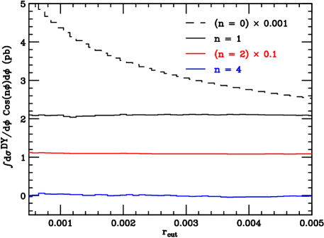
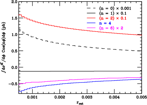
Figure 1: Lowest-order harmonics as a function of $r_{\rm cut}=q_{\rm cut}/M$ in the cases of DY lepton pair (left) and $t\bar{t}$ (right) production at the LHC.

In Fig. 1-left we also report the result for the $n=0$ harmonic (dashed line) of ‘$Z+1$ parton’ production. The $n=0$ harmonic corresponds to the total (azimuthally-integrated) cross section, and it receives contributions from both real and virtual emission subprocesses. Real and virtual terms are separately divergent and their divergences cancel in the total contribution. In Fig. 1-left we report the result of the $n=0$ harmonic computed exactly as specified in Eq. (11), namely, by applying a non-vanishing lower limit $q_{\rm cut}=r_{\rm cut}M$ on $q_{T}$. Therefore, our computation selects only the real-emission term due to the ‘$Z+1$ parton’ subprocesses. As is well known (see also Sect. 4.1), this real-emission term diverges in the limit $q_{\rm cut}\rightarrow 0$ and the divergent behaviour is proportional to $\ln^{2}r_{\rm cut}$: in Fig. 1-left we clearly see the increasing behaviour of the $n=0$ harmonic as $r_{\rm cut}\rightarrow 0$. In the actual computation of the total cross section, the $n=0$ result in Fig. 1-left has to be combined with the NLO real-emission term at still smaller values of $r_{\rm cut}$ and with the LO and NLO virtual terms, thus leading to a total finite result. For the sake of completeness, we report the value (including the numerical error of the Monte Carlo integration) of the NLO total cross section $\sigma_{DY}^{NLO}$ that we obtain by using the same parameters as used in the results of Fig. 1-left: it is $\sigma_{DY}^{NLO}=1100\pm 1$ pb. We note that $\sigma_{DY}^{NLO}$ is roughly 100 times larger than the value of the $\cos(2\varphi)$ asymmetry in Fig. 1-left.

The DY process is quite ‘special’ with respect to azimuthal correlations: the azimuthal correlations are finite order-by-order in QCD perturbation theory and their general QCD structure involves only 4 azimuthal harmonics (as shown in Eq. (12)). For most of the other hard-scattering processes (with few possible exceptions such as $H\rightarrow\gamma\gamma,ZZ$ production, as discussed in Sect. 2) azimuthal correlations behave differently: usually they have an azimuthal dependence that involves an infinite set of harmonics (all values of $n$) and in many cases f.o. QCD computations lead to divergences.

We consider the production of heavy-quark $Q{\bar{Q}}$ pairs and we treat the heavy quark and antiquark as on-shell particles. Our discussion equally applies to any heavy quark, but we specifically consider top quarks since the on-shell treatment is more suitable in this case. In Fig. 1-right we present results for $t{\bar{t}}$ production that are obtained analogously to the DY results presented in Fig. 1-left.

Our QCD computation of $t{\bar{t}}$ production is performed by using the numerical Monte Carlo program of Ref. [22], which includes QCD radiative corrections at NLO (it uses the NLO scattering amplitudes of the MCFM program [23]) and part of the NNLO contributions. We set $\mu_{F}=\mu_{R}=m_{t}$ and we use the value $m_{t}=173.3$ GeV for the mass $m_{t}$ of the top quark. We consider the azimuthal angle $\varphi$ of the top quark in the CS frame, and in Fig. 1-right we present the numerical results of various $\cos(n\varphi)$ asymmetries (see Eq. (11)) after their integration over the invariant mass $M$ of the $t{\bar{t}}$ pair. As in the case of the results in Fig. 1-left, the $t{\bar{t}}$ results are integrated over the polar angle of the top quark and over the rapidity $y$ and transverse momentum $q_{T}$ ($q_{T}>q_{\rm cut}$) of the $t{\bar{t}}$ pair. The azimuthal asymmetries are evaluated (as a function of $r_{\rm cut}=q_{\rm cut}/M$) at their non-trivial lowest order (i.e., ${\cal O}(\alpha_{\mathrm{S}}^{3})$) in f.o. perturbation theory and, therefore, we compute all the NLO tree-level partonic processes whose final state is ‘$t{\bar{t}}+1$ parton’.

Before commenting on the results in Fig. 1-right, we recall some of the results in Ref. [12]. In Ref. [12] azimuthal correlations for $t{\bar{t}}$ production are computed in analytic form in the small-$q_{T}$ limit. At ${\cal O}(\alpha_{\mathrm{S}}^{3})$ the result of Ref. [12] shows that the $q_{T}$-dependent azimuthal-correlation cross section $d\sigma^{\rm corr}/dq_{T}^{2}d\varphi$ behaves proportionally to $1/q_{T}^{2}$ in the limit $q_{T}\rightarrow 0$ and, hence, it is not integrable over $q_{T}$ down to the region where $q_{T}=0$. The $1/q_{T}^{2}$ behaviour is proportional to a non-polynomial function of $\cos^{2}\varphi$ that, therefore, leads to divergent $\cos(n\varphi)$ harmonics for even values of $n$ $(n=2,4,6,\dots)$. The $q_{T}$ spectra of harmonics with odd values of $n$ have instead a less singular $q_{T}$ behaviour at ${\cal O}(\alpha_{\mathrm{S}}^{3})$ and they are integrable over $q_{T}$ in the limit $q_{T}\rightarrow 0$.

The numerical results in Fig. 1-right are consistent with the convergent or divergent behaviour predicted in Ref. [12]. The harmonic with $n=1$ (black line) is not vanishing and basically independent of $r_{\rm cut}$ for very small values of $r_{\rm cut}$. The sign of the $n=1$ harmonic is negative (the $n=1$ harmonic of $\bar{t}$ would be positive, analogously to the corresponding harmonic of the electron in the DY case of Fig. 1-left), and its absolute size (note that it is rescaled by a factor of 0.1 in Fig. 1-right) is roughly a factor of two smaller than the size of the $n=1$ harmonic for $Z(e^{+}e^{-})$ production (Fig. 1-left). The harmonics with $n=2$ (red line), $n=4$ (blue line) and $n=6$ (magenta line) in Fig. 1-right have instead an increasing (in absolute value) size for small and decreasing values of $r_{\rm cut}$: this behaviour is consistent with a $\ln r_{\rm cut}$ dependence, as expected from the analytical results in Ref. [12]. The results for $n=2,4$ and 6 in Fig. 1-right have no straightforward quantitative implications for physical azimuthal asymmetries since they refer to small values of $r_{\rm cut}$ (and they eventually diverge in the limit $r_{\rm cut}\rightarrow 0$). Nonetheless we observe that the absolute magnitude of the $n$-even $\cos(n\varphi)$ asymmetries decreases as $n$ increases. As in the case of Fig. 1-left for the DY process, in Fig. 1-right we also present the ${\cal O}(\alpha_{\mathrm{S}}^{3})$ result of the $n=0$ harmonic (dashed line) for the real-emission process ‘$t{\bar{t}}+1$ parton’. Analogously to the DY process, the ‘$t{\bar{t}}+1$ parton’ contribution to the $n=0$ harmonic diverges in the limit $r_{\rm cut}\rightarrow 0$, and its dominant behaviour at small $r_{\rm cut}$ is proportional to $\ln^{2}r_{\rm cut}+{\cal O}(\ln r_{\rm cut})$. At small values of $r_{\rm cut}$ the shape of the $r_{\rm cut}$-dependence of the $n=0$ result is thus steeper than that of the results for the harmonics with $n=2,4$ and 6. After combining real and virtual contributions, the $n=0$ harmonic gives the total cross section. The value (including the numerical error of the Monte Carlo integration) of the NLO total cross section that we find is $\sigma_{t{\bar{t}}}^{NLO}=226.2\pm 0.1$ pb. We note that $\sigma_{t{\bar{t}}}^{NLO}$ is roughly 200 times larger than the absolute value of the $\cos\varphi$ asymmetry ($n=1$) in Fig. 1-right.

As we have anticipated in Sect. 2 with a brief sentence, we expect (and predict) the appearance of f.o. perturbative divergences in the computation of QED radiative corrections to azimuthal correlations for the DY process. To explicitly explain this point we consider some analogies of the DY and $t{\bar{t}}$ production processes. We have illustrated the ${\cal O}(\alpha_{\mathrm{S}}^{3})$ divergences of the $n$-even $\cos(n\varphi)$ asymmetries for $t{\bar{t}}$ production. Part of these divergences arise from the computation of the partonic subprocess $q{\bar{q}}\rightarrow t{\bar{t}}+g$ and, specifically, they arise from the kinematical region where the radiated final-state gluon $g$ is soft and at wide angle with respect to the direction of the initial-state $q$ and ${\bar{q}}$. From this kinematical region the $t{\bar{t}}$ spectrum $d\sigma/dq_{T}^{2}d\varphi$ receives an azimuthal-correlation contribution that behaves as $1/q_{T}^{2}$ and that depends on the QCD colour charges of the final-state $t$ and $\bar{t}$. Specifically, this contribution is proportional to the Fourier transformation of the function ${\bf D}^{(1)}$ in Eq. (36) of Ref. [12]. The first-order QED radiative corrections to the DY process involve analogous partonic processes, such as $q{\bar{q}}\rightarrow Z(e^{+}e^{-})+\gamma$, with a soft and wide-angle photon $\gamma$ that is radiated in the final state. These photon radiative corrections produce f.o. QED divergences to azimuthal asymmetries for the DY process. The DY analogue of the $t{\bar{t}}$ function ${\bf D}^{(1)}$ in Eq. (36) of Ref. [12] is simply obtained by replacing the QCD colour charges of $t$ and ${\bar{t}}$ with the QED electric charges of the DY final-state leptons (by simple inspection of Eq. (36) in Ref. [12], such replacement leads to a non-vanishing result).

More generally, we remark that the expression in Eq. (12) for the DY process is valid only at the Born level with respect to the EW interactions (although the expression is valid at arbitrary orders in QCD perturbation theory). Including QED radiative corrections, we conclude that the azimuthal-correlation cross section $d\sigma_{DY}/dq_{T}^{2}d\varphi$ for the DY process receives contributions from $\cos(n\varphi)$ and $\sin(n\varphi)$ harmonics with arbitrary values of $n$ (not only $n=1,2$ as in Eq. (12)). Moreover, the lowest-order perturbative QED computation of the $\cos(n\varphi)$ contributions with $n$-even already leads to a singular (not integrable) behaviour in the limit $q_{T}\rightarrow 0$ and to ensuing divergent azimuthal asymmetries upon integration over $q_{T}$. The divergences are switched on by QED radiative corrections and can receive additional contributions from powers of $\alpha_{\mathrm{S}}$ in the context of mixed QED$\times$QCD radiative corrections. Obviously, similar divergences arise also in a pure QED context such as, for instance, in the QED computation of the process $e^{+}e^{-}\rightarrow\mu^{+}\mu^{-}+X$. Eventually all these divergences originate from the QED analogue of the condition (10): the QED divergences arise if ‘at least one the final-state particles with momenta $p_{3}$ and $p_{4}$ carries non-vanishing electric charge’.

We note that lepton pairs with high invariant mass can also be produced throughout the partonic subprocess $\gamma\gamma\rightarrow\ell^{+}\ell^{-}$, in which the initial-state colliding photons arise from the photon PDF of the colliding hadrons. Strictly speaking, lepton pairs that are produced in this way are not physically distinguishable from those that are produced by the DY mechanism of quark–antiquark annihilation. Since the ratio between the photon PDF and the quark (or antiquark) PDF is formally of ${\cal O}(\alpha/\alpha_{\mathrm{S}})$ ($\alpha$ is the fine structure constant), the subprocess $\gamma\gamma\rightarrow\ell^{+}\ell^{-}$ can be regarded as a QED radiative correction in the context of the DY process. We remark that radiative corrections to $\gamma\gamma\rightarrow\ell^{+}\ell^{-}$ also produce divergences in the computation of the lepton azimuthal correlations. These divergences (see Sect. 5.1) originate from the abelian (photonic) analogue of the condition (9): the divergences arise if ‘at least one of the initial-state colliding partons $c_{1}$ and $c_{2}$ is a photon’.

To cure the f.o. perturbative divergences of azimuthal correlations one may advocate non-perturbative strong-interactions dynamics and related non-perturbative QCD effects, which can be sizeable in the small-$q_{T}$ region. However, in the case of $q_{T}$-integrated azimuthal correlations (see Eq. (7)) the non-perturbative QCD dynamics should cancel divergent terms proportional to some powers of $\alpha_{\mathrm{S}}(M)$, and this would imply that non-perturbative QCD effects scale logarithmically with $M$ (i.e., these effects would not be suppressed by some power of $\Lambda_{QCD}/M$ in the hard-scattering regime $M\gg\Lambda_{QCD}$), thus spoiling not only the finiteness but also the infrared safety of the azimuthal correlations. Moreover such non-perturbative cure of the divergent behaviour cannot be effective in the case of QED radiative corrections and, in particular, it cannot be conceptually at work in a pure QED context since QED is well-behaved in the infrared (small-$q_{T}$) region. In the following Sections we show that the problem of f.o. divergences in azimuthal correlations has a satisfactory solution entirely within the context of perturbation theory. Namely, the resummation of perturbative corrections to all orders leads to ($q_{T}$ integrated) azimuthal asymmetries that are finite and computable. Such solution is effective in both QCD and QED contexts, although in the QCD case this does not imply that the non-perturbative effects have a negligible quantitative role in the small-$q_{T}$ region.

4 The small-$q_{T}$ region

The f.o. divergences of azimuthal correlations arise from the small-$q_{T}$ region and, eventually, from the $q_{T}$ behaviour at the phase space point where $q_{T}=0$. From a physical viewpoint, however, a single (isolated) phase space point is harmless and, in particular, non-vanishing azimuthal correlations (which are defined with respect to the direction of $q_{T}$) cannot be measured if $q_{T}\sim 0$. These physical requirements imply that the $q_{T}$ dependence of azimuthal-correlation observables has to be sufficiently smooth in the small-$q_{T}$ region and, in particular, in the limit $q_{T}\rightarrow 0$.

We specify more formally these smoothness requirements. Since physical measurements cannot be performed at a single phase space point, we split the $q_{T}$ integration region in the two intervals where $0\leq q_{T}\leq q_{\rm cut}$ (the lower-$q_{T}$ bin) and $q_{T}\geq q_{\rm cut}$ (the higher-$q_{T}$ region). We then consider a generic azimuthal-correlation observable (e.g., multidifferential cross sections as in Eqs. (3) and (4), or $n$-th harmonics as in Eq. (11)) and we denote by $\sigma_{l}(q_{\rm cut};\varphi)$ and $\sigma_{h}(q_{\rm cut};\varphi)$ the ‘cross sections’ that are obtained by $q_{T}$ integration of the observable over the lower-$q_{T}$ bin and the higher-$q_{T}$ region, respectively. The smoothness requirements are

$$\lim_{q_{\rm cut}\rightarrow 0}\;\sigma_{l}(q_{\rm cut};\varphi)=0\;\;,$$ (13)

$$\lim_{q_{\rm cut}\rightarrow 0}\;\sigma_{h}(q_{\rm cut};\varphi)=\sigma_{\rm tot}(\varphi)\;\;,$$ (14)

where $\sigma_{\rm tot}(\varphi)$ denotes the ‘total’ cross section (i.e., the result obtained by integrating the observable over the entire region of $q_{T}$). These requirements specify azimuthal correlations that are physically well behaved. In particular, Eq. (13) implies that non-vanishing azimuthal correlations cannot be physically observed if $q_{T}\sim 0$, and Eq. (14) implies that the total azimuthal correlation is physically observable. Note, however, that Eqs. (13) and (14) do not specify how $d\sigma/dq_{T}^{2}d\varphi$ exactly behaves in the limit $q_{T}\rightarrow 0$. Nonetheless, Eqs. (13) and (14) imply that the sole phase space point at $q_{T}=0$ (where azimuthal-correlation angles are not defined) has no relevant physical role (the lower-$q_{T}$ bin has an analogous harmless role if $q_{\rm cut}$ is sufficiently small).

The f.o. divergences of azimuthal-correlation observables are due to the fact that $d\sigma/dq_{T}^{2}d\varphi$ does not have a (‘sufficiently’) smooth dependence on $q_{T}$ at small values of $q_{T}$ if this quantity is computed order-by-order in perturbation theory. In particular, $\sigma_{h}(q_{\rm cut};\varphi)$ diverges in the limit $q_{\rm cut}\rightarrow 0$ and, consequently, $\sigma_{\rm tot}(\varphi)$ is not computable, whereas $\sigma_{l}(q_{\rm cut};\varphi)$ is definitely not computable (divergent) even if $q_{\rm cut}$ has a finite value.

As we have observed in Sect. 3, also the customary azimuthally-integrated (or azimuthally-averaged) cross section (i.e., the harmonic with $n=0$ in Eq. (11) or Fig. 1) does not fulfil the requirements in Eqs. (13) and (14) (both $\langle\sigma_{l}(q_{\rm cut};\varphi)\rangle_{\rm av.}$ and $\langle\sigma_{h}(q_{\rm cut};\varphi)\rangle_{\rm av.}$ can separately be divergent in the limit $q_{\rm cut}\rightarrow 0$). Therefore, the f.o. calculation of azimuthally-integrated cross section can have difficulties (as is well known) in describing the detailed $q_{T}$ shape in the small-$q_{T}$ region. In contrast to azimuthal-correlations observables, however, both $\langle\sigma_{l}(q_{\rm cut};\varphi)\rangle_{\rm av.}$ and $\langle\sigma_{h}(q_{\rm cut};\varphi)\rangle_{\rm av.}$ are computable for finite values of $q_{\rm cut}$. In particular, the total cross section $\langle\sigma_{\rm tot}(q_{\rm cut};\varphi)\rangle_{\rm av.}=\langle\sigma_{l}(q_{\rm cut};\varphi)\rangle_{\rm av.}+\langle\sigma_{h}(q_{\rm cut};\varphi)\rangle_{\rm av.}$ is always finite and computable (for arbitrary non-vanishing values of $q_{\rm cut}$) within f.o. perturbation theory.

In the following sections we discuss the small-$q_{T}$ behaviour of cross sections in f.o. perturbation theory and after all-order resummation.

4.1 Perturbative expansion with azimuthal-correlation terms

Among all the hadroproduction processes of the type in Eq. (1), we consider those that at the LO in perturbative QCD are produced by the following partonic subprocesses:

$$c_{1}+c_{2}\rightarrow F(\{p_{3},p_{4}\})\;\;,$$ (15)

where $c_{1}$ and $c_{2}$ $(c_{i}=q,{\bar{q}},g)$ are the initial-state massless colliding partons of the two hadrons $h_{1}$ and $h_{2}$. In the case in which one or both particles (with momenta $p_{3},p_{4}$) in $F$ is a jet, the notation in Eq. (15) means that the jet is replaced by a corresponding QCD parton. Note that the LO process in Eq. (15) is an ‘elastic’ production process, in the sense that $F$ is not accompanied by any additional final-state radiation. This specification is not trivial, since it excludes some processes from our ensuing considerations. Some processes are excluded because of quantum number conservation. For instance, if $F$ includes two top quarks (not a $t{\bar{t}}$ pair) no LO process as in Eq. (15) is permitted by flavour conservation. Some other processes are excluded because of their customary perturbative QCD treatment. For instance, if $F$ contains a hadron, its QCD treatment requires the introduction of a corresponding fragmentation function and, consequently, $F$ is necessarily produced with accompanying fragmentation products in the final state. Therefore, in the following we exclude the cases in which $F$ includes one or two hadrons. All the processes that are explicitly listed in Eq. (6) (including the DY process) have LO partonic processes of the type in Eq. (15).

The small-$q_{T}$ behaviour of azimuthal correlations for the processes that we have just specified is partly related to the behaviour of $q_{T}$ differential cross sections that are integrated over the entire azimuthal-angle region (or, equivalently, that are azimuthally averaged). The behaviour in the azimuthally-integrated (averaged) case is well known (starting from some of the ‘classical’ studies for the DY process [24, 25, 26, 27, 28]), and in our presentation we contrast it with the cases with divergent azimuthal correlations. To remark the differences between the two cases in general terms, we use a shorthand notation, which can be applied to final-state systems $F$ with two or more particles (a more refined kinematical notation can be found in Refs. [11, 12]). A generic multidifferential cross section (e.g., Eq. (3), Eq. (4) or related observables) with dependence on $q_{T}$ and on the azimuthal-correlation angle is simply denoted by $d\sigma/dM^{2}d^{2}{{\mbox{\boldmath$q_{T}$}}}$, where $q_{T}$ is the transverse momentum of $F$. Additional kinematical variables that are possibly not integrated (such as rapidities and polar angles) are not explicitly denoted. The dependence on a generic (as discussed in Sect. 2) azimuthal-correlation angle with respect to $q_{T}$ is denoted through the dependence on the direction ${\mbox{\boldmath${\hat{q}}_{T}$}}={{\mbox{\boldmath$q_{T}$}}}/q_{T}$ of the two-dimensional vector $q_{T}$. In practice such dependence will occur through functions of scalar quantities such as, for instance, ${\mbox{\boldmath${\hat{q}}_{T}$}}\cdot{\bf p}_{3{\bf T}}$. In particular, independent of ${\hat{q}}_{T}$ means absence of azimuthal correlations, and the azimuthally-integrated (averaged) cross section corresponds to the azimuthal integration (average) with respect to the direction ${\hat{q}}_{T}$ of $q_{T}$.

Owing to transverse-momentum conservation in the process of Eq. (15), at the LO level $F$ is produced with vanishing $q_{T}$. Its corresponding LO $q_{T}$ cross section is proportional to $\delta^{(2)}({\mbox{\boldmath$q_{T}$}})$,

$$\frac{d\sigma^{LO}}{dM^{2}\,d^{2}{{\mbox{\boldmath$q_{T}$}}}}\propto\delta^{(2)}({\mbox{\boldmath$q_{T}$}})\;\;,$$ (16)

and the proportionality factor is simply the LO total ($q_{T}$ integrated) cross section. In the presence of the LO sharp $q_{T}$ behaviour of Eq. (16), NLO QCD radiative corrections are dynamically enhanced in the small-$q_{T}$ region. The dynamical enhancement is due to QCD radiation of low transverse-momentum partons (soft gluons or QCD partons that are collinear to the initial-state colliding partons), and it has the following general form:

$$\frac{d\sigma^{NLO}}{dM^{2}d^{2}{{\mbox{\boldmath$q_{T}$}}}}\propto\delta^{(2)}({\mbox{\boldmath$q_{T}$}})+\alpha_{\mathrm{S}}\left\{\left(a_{2}\left[\frac{1}{q_{T}^{2}}\ln\left(\frac{M^{2}}{q_{T}^{2}}\right)\right]_{+}+a_{1}\left[\frac{1}{q_{T}^{2}}\right]_{+}+a_{0}\;\delta^{(2)}({\mbox{\boldmath$q_{T}$}})+\frac{a_{\rm corr}({\mbox{\boldmath${\hat{q}}_{T}$}})}{q_{T}^{2}}\right)+\dots\right\}\;,$$ (17)

where the dots on the right-hand side denote contributions that are less enhanced (‘non-singular’) in the limit $q_{T}\rightarrow 0$. The ‘coefficients’ $a_{i}$ ($i=0,1,2$) and $a_{\rm corr}$ in Eq. (17) depend on the process and they are independent of $q_{T}$ (we mean they are independent of the magnitude $q_{T}$ of the vector $q_{T}$). The important point (see below) is that $a_{\rm corr}$ does depend on the direction ${\hat{q}}_{T}$ of $q_{T}$, whereas $a_{i}$ ($i=0,1,2$) do not depend on it. All these coefficients ($a_{1},a_{2}.a_{3},a_{\rm corr}$) can depend on the other kinematical variables (e.g., rapidities and polar angles). The QCD running coupling $\alpha_{\mathrm{S}}$ in Eq. (17) and in all the subsequent formulae is evaluated at a scale of the order of $M$ (e.g., we can simply assume $\alpha_{\mathrm{S}}=\alpha_{\mathrm{S}}(M)$).

The terms that we have explicitly written in the right-hand side of Eq. (17) scale as $1/q_{T}^{2}$ (modulo logs) in the limit $q_{T}\rightarrow 0$ (i.e., they scale as $1/\lambda^{2}$ under the replacement ${\mbox{\boldmath$q_{T}$}}\rightarrow\lambda{\mbox{\boldmath$q_{T}$}}$). The non-singular terms (which are simply denoted by the dots) represent subdominant (‘power-correction’) contributions in the limit $q_{T}\rightarrow 0$. These are, for instance, terms of the type $M/q_{T}$ or, more generally, terms that are relatively suppressed by some powers (modulo logs) of $q_{T}/M$. Independently of their specific form and of their azimuthal dependence, these non-singular terms have an integrable and smooth behaviour in the limit $q_{T}\rightarrow 0$. Because of these features, the non-singular terms and the ensuing azimuthal-correlation effects are well behaved in the small-$q_{T}$ region. Note, however, that the non-singular terms produce azimuthal effects whose actual size (and $q_{T}$ behaviour) depends on the specific definition of the azimuthal-correlation angle (see Eq. (8) and related comments in Sect. 2).

The expression in Eq. (17) is the master formula that we use for our discussion of the small-$q_{T}$ behaviour of azimuthal correlations at NLO and higher orders. Considering the ‘singular’ terms (the NLO terms that scale as $1/q_{T}^{2}$, modulo logs, in the limit $q_{T}\rightarrow 0$), the azimuthal dependence is entirely embodied in $a_{\rm corr}({\mbox{\boldmath${\hat{q}}_{T}$}})$. More precisely, the azimuthal-correlation dependence has been separated (as in Eq. (7)) and embodied in $a_{\rm corr}({\mbox{\boldmath${\hat{q}}_{T}$}})$ that, therefore, gives a vanishing result after azimuthal integration. Using the notation in Eq. (7) we have

$$\langle a_{\rm corr}({\mbox{\boldmath${\hat{q}}_{T}$}})\rangle_{\rm av.}=0\;\;.$$ (18)

This azimuthal-correlation term is absent for the DY process (i.e., $a_{\rm corr}({\mbox{\boldmath${\hat{q}}_{T}$}})=0$ in this case), and in all the other processes it has no effect by considering $q_{T}$ dependent but azimuthally-integrated observables. The presence of such term produces a $q_{T}$ behaviour that definitely differs from the behaviour studied in the ‘classical’ literature [24, 25, 26, 27, 28] on the small-$q_{T}$ region and on QCD transverse-momentum resummation.

The other (‘classical’) terms in Eq. (17) are proportional to the coefficients $a_{i}$ ($i=0,1,2$), and the symbol $[~{}~{}]_{+}$ denotes the (‘singular’) ‘plus’-distribution, which is defined by its action onto any smooth function $f({\mbox{\boldmath$q_{T}$}})$ of $q_{T}$. The definition is

$$\int_{0}^{+\infty}d^{2}{\mbox{\boldmath$q_{T}$}}\;\,f({\mbox{\boldmath$q_{T}$}})\;\left[g({\mbox{\boldmath$q_{T}$}})\right]_{+}\equiv\int_{0}^{+\infty}d^{2}{\mbox{\boldmath$q_{T}$}}\,\left[f({\mbox{\boldmath$q_{T}$}})-f({\bf 0})\,\theta(\mu_{0}-q_{T})\right]\;g({\mbox{\boldmath$q_{T}$}})\;\;,$$ (19)

where $g({\mbox{\boldmath$q_{T}$}})=\frac{1}{q_{T}^{2}}\ln^{m}(M^{2}/q_{T}^{2})$ ($m=0,1$) in Eq. (17), and $\mu_{0}$ is a scale of the order of $M$ (at the formal level, varying the value of $\mu_{0}$ changes the plus-distributions and the coefficient $a_{0}$, so that the right-hand side of Eq. (17) is unchanged). The plus-distribution in Eq. (19) is equivalently defined through a limit procedure as follows:

$$\left[g({\mbox{\boldmath$q_{T}$}})\right]_{+}=\lim_{q_{0}\rightarrow 0}\left[\theta(q_{T}-q_{0})\;g({\mbox{\boldmath$q_{T}$}})-\delta^{(2)}({\mbox{\boldmath$q_{T}$}})\int d^{2}{\bf k_{T}}\;g({\bf k_{T}})\;\theta(\mu_{0}-k_{T})\,\theta(k_{T}-q_{0})\right]\;\;.$$ (20)

Note that the point at $q_{T}=0$ is at the border of the phase space, but, at the strictly formal level, it is inside the phase space (at variance with the case of azimuthal correlations, in which it is formally outside the phase space). This is essential to make sense of the LO $q_{T}$ differential cross section in Eq. (16) and of the corresponding LO total cross section. This is also essential (see Eqs. (19) and (20)) to transform the non-integrable $q_{T}$ behaviour of $\frac{1}{q_{T}^{2}}\ln^{m}(M^{2}/q_{T}^{2})$ into an integrable plus-distribution over the small-$q_{T}$ region. The plus-distribution $[~{}g({\mbox{\boldmath$q_{T}$}})~{}]_{+}$ involves two terms: a term that is simply proportional to the function $g({\mbox{\boldmath$q_{T}$}})$ and a contact term (the term proportional to $f({\bf 0})$ in Eq. (19) or, equivalently, the term proportional to $\delta^{(2)}({\mbox{\boldmath$q_{T}$}})$ in Eq. (20)). At the conceptual level, these two terms arise from a combination of real and virtual radiative corrections, which are separately infrared divergent. Real (soft and collinear) emission corrections to the LO process in Eq. (15) produce the non-integrable terms $\frac{1}{q_{T}^{2}}\ln^{m}(M^{2}/q_{T}^{2})$, while the corresponding virtual radiative corrections lead to the contact terms that eventually regularize the divergence at $q_{T}=0$.

The azimuthal-correlation term in Eq. (17) is instead proportional to the divergent (not integrable) function $1/q_{T}^{2}$, rather than to a corresponding plus-distribution. At the formal level one may be tempted to transform the azimuthal-correlation term into a plus-distribution through the replacement $a_{\rm corr}({\mbox{\boldmath${\hat{q}}_{T}$}})/q_{T}^{2}\rightarrow[~{}a_{\rm corr}({\mbox{\boldmath${\hat{q}}_{T}$}})/q_{T}^{2}~{}]_{+}$, but such a replacement would not be effective since

$$\left[\frac{a_{\rm corr}({\mbox{\boldmath${\hat{q}}_{T}$}})}{q_{T}^{2}}\right]_{+}=\frac{a_{\rm corr}({\mbox{\boldmath${\hat{q}}_{T}$}})}{q_{T}^{2}}\;\;,$$ (21)

namely, the plus-prescription is not able to regularize the non-integrable behaviour of azimuthal-correlation terms. The equality in Eq. (21) is a consequence of the fact that the contact term (see Eq. (20)) in the corresponding plus-prescription identically vanishes: indeed we have

$$\delta^{(2)}({\mbox{\boldmath$q_{T}$}})\int d^{2}{\bf{k_{T}}}\;\frac{a_{\rm corr}({\mbox{\boldmath${\hat{k}}_{T}$}})}{k_{T}^{2}}\;\theta(\mu_{0}-k_{T})\,\theta(k_{T}-q_{0})=0\;\;,$$ (22)

because the azimuthal integration of $a_{\rm corr}({\mbox{\boldmath${\hat{k}}_{T}$}})$ gives a vanishing result (see Eq. (18)). We note that a result analogous to Eq. (21), namely

$$\left[g_{\rm corr}({\mbox{\boldmath$q_{T}$}})\right]_{+}=g_{\rm corr}({\mbox{\boldmath$q_{T}$}})\;\;,$$ (23)

is valid for any azimuthal-correlation function $g_{\rm corr}({\mbox{\boldmath$q_{T}$}})$, i.e., any function such that $\langle g_{\rm corr}({\mbox{\boldmath$q_{T}$}})\rangle_{\rm av.}~{}=~{}0$. Therefore, in general we can conclude that azimuthal-correlation terms that are not integrable in the limit $q_{T}\rightarrow 0$ cannot be regularized by the plus-prescription. This general conclusion and, in particular, the equality in Eq. (21) have a simple conceptual interpretation in the context of f.o. perturbation theory. Virtual radiative corrections to the process in Eq. (15) have $q_{T}=0$ and, therefore, they cannot contribute to azimuthal-correlation terms. In particular, they cannot provide the real-emission azimuthal-correlation term with a (non-vanishing) contact term that transforms the non-integrable real-emission contribution into an integrable plus-distribution. In summary, the azimuthal correlation of the $q_{T}$ cross section is a phenomenon that is necessarily produced by real emission (since azimuthal dependence requires $q_{T}\neq 0$) and the f.o. divergences of the azimuthal asymmetries are the consequence of a complete mismatch with virtual emission, which is completely absent (i.e., it does not contribute) at the corresponding perturbative order. In the case of azimuthal-independent (plus-distribution) terms, instead, both real and virtual effects contribute at the NLO, although their relative contribution is highly unbalanced in the small-$q_{T}$ region.

The $r_{\rm cut}$ ($q_{\rm cut}$) dependence of the results that are presented in Fig. 1 is fully consistent with the small-$q_{T}$ behaviour in Eq. (17). The harmonics with $n\neq 0$ receive contributions only from the term that is proportional to $a_{\rm corr}({\mbox{\boldmath${\hat{q}}_{T}$}})$ in Eq. (17), while $a_{\rm corr}({\mbox{\boldmath${\hat{q}}_{T}$}})$ does not contribute to the $n=0$ harmonics (because of Eq. (18)). We simply note that in the DY process we have $a_{\rm corr}({\mbox{\boldmath${\hat{q}}_{T}$}})=0$, whereas in the case of $t{\bar{t}}$ production $a_{\rm corr}({\mbox{\boldmath${\hat{q}}_{T}$}})$ is not vanishing (in particular, the $n=1$ harmonic of $a_{\rm corr}({\mbox{\boldmath${\hat{q}}_{T}$}})$ vanishes, while $a_{\rm corr}({\mbox{\boldmath${\hat{q}}_{T}$}})$ has non-vanishing harmonics with $n=2,4,6$). We also note that the results for the harmonics with $n=0$ (in both the DY and $t{\bar{t}}$ production processes) follow from the $q_{T}$ shape of the plus-distribution terms in Eq. (17): the $q_{T}$ integration of the plus-distributions over the region $q_{T}>q_{\rm cut}=r_{\rm cut}M$ produces the $r_{\rm cut}$ dependence in Fig. 1, and this $r_{\rm cut}$ dependence is exactly cancelled by that produced from the integration of the plus-distributions over the region $0\leq q_{T}\leq q_{\rm cut}$.

We include a comment on an additional point related to the f.o. perturbative expansion of generic hard-scattering processes. In our discussion of Eq. (17), we have considered processes that at the LO are initiated by the partonic subprocesses in Eq. (15). We note that elastic production processes of the type in Eq. (15) can also appear at some higher perturbative orders. For instance, as already mentioned in Sect. 2, this is the case if $F=\{\gamma\gamma\},\{ZZ\},\{W^{+}W^{-}\}$. These diboson production processes are initiated at LO by $q{\bar{q}}\rightarrow F$, and they also receive contributions from $gg\rightarrow F$ (the gluons are coupled to $\gamma\gamma,ZZ,W^{+}W^{-}$ through a quark loop) starting from the NNLO. In these cases, the next-order radiative corrections to $gg\rightarrow F$ produce a small-$q_{T}$ behaviour that has exactly the same structure as that in the round-bracket term of Eq. (17). Our following discussion throughout the paper equally applies to all the processes that can occur through subprocesses of the type in Eq. (15) at some perturbative order (different types of colliding partons $c_{1}$ and $c_{2}$ can be involved at different perturbative orders).

Small-$q_{T}$ singular terms of the type in Eq. (17) are present in the computation of $d\sigma/dM^{2}d^{2}{{\mbox{\boldmath$q_{T}$}}}$ at each higher perturbative orders. The $1/q_{T}^{2}$ behaviour of both azimuthally-independent and azimuthally-correlated terms is enhanced by logarithmic factors, $\ln^{k}(M^{2}/q_{T}^{2})$, produced by multiple radiation of soft and collinear partons. There are at most two additional powers of $\ln(M^{2}/q_{T}^{2})$ for each additional power of $\alpha_{\mathrm{S}}$, so that the dominant singular terms have a double-logarithmic structure. The N^kLO radiative corrections to $d\sigma/dM^{2}d^{2}{{\mbox{\boldmath$q_{T}$}}}$ include singular terms that are proportional to $\alpha_{\mathrm{S}}^{k}\frac{1}{q_{T}^{2}}\ln^{m}(M^{2}/q_{T}^{2})$ (with $m\leq 2k-1$), and this $q_{T}$ dependence is regularized by a plus-prescription only in the case of azimuthally-independent contributions. Owing to Eq. (23), the plus-prescription is not effective for azimuthal-correlation terms.

The order-by-order singular behaviour that we have just discussed poses no problems for a basic quantity such as the total ($q_{T}$ and azimuthally integrated) cross section: the singular azimuthal-correlation terms cancel because of the azimuthal integration, and the plus-distribution terms are integrable over $q_{T}$. As is well known, the plus-distribution terms (which remain after azimuthal integration) are not ‘harmless’ for differential cross sections. They lead to a sharp unphysical behaviour of the small-$q_{T}$ differential cross section at the NLO, and to large radiative-correction effects at any subsequent perturbative order, with an unstable f.o. expansion and poor predictivity for the detailed shape of the $q_{T}$ cross section in the small-$q_{T}$ region. The smooth physical behaviour of the $q_{T}$ cross section and the predictivity of perturbative QCD can be recovered by the all-order resummation (transverse-momentum resummation) of the logarithmically-enhanced plus-distribution terms.

In the case of azimuthally-sensitive observables, the disease of f.o. perturbation theory is more serious. The singular azimuthal-correlation terms are not integrable and, as discussed in Sect. 2, basic quantities such as the total ($q_{T}$ integrated) cross section at fixed azimuthal angle (see Eq. (6)) and the total ($q_{T}$ integrated) azimuthal asymmetries (see Eq. (11)) can be divergent if they are evaluated in f.o. perturbation theory. In the presence of divergences, also the f.o. perturbative result for $d\sigma^{\rm corr}/dM^{2}d^{2}{{\mbox{\boldmath$q_{T}$}}}$ at fixed (and finite) values of $q_{T}$ has an unphysical shape in the small-$q_{T}$ region, since the f.o. result follows a non-integrable (unphysical) behaviour.

In the following we briefly recall known results on transverse-momentum resummation for ‘azimuthally-insensitive’ observables. More precisely, we simply sketch some main points of transverse-momentum resummation that are relevant for our subsequent discussion on azimuthal correlations and asymmetries.

4.2 Transverse-momentum resummation with no divergent azimuthal correlations

In this subsection we limit ourselves to considering only singular contributions to $d\sigma/dM^{2}d^{2}{{\mbox{\boldmath$q_{T}$}}}$ that are independent of the azimuthal-correlation angles. Order-by-order in perturbation theory, these contributions can be additively separated from non-singular terms (see, e.g., the ‘dots’ in the right-hand side of Eq. (17)), and they can also be additively separated from singular azimuthal-correlation terms (see Eqs. (7), (17), (23) and accompanying comments). Therefore, we are dealing with all the singular plus-distribution terms that appear in Eq. (17) and in corresponding higher-order contributions. As a consequence of the additive separability, azimuthally-insensitive, azimuthally-integrated and azimuthally-averaged contributions have the same equivalent meaning in the context of the discussion in this subsection. In the case of processes whose azimuthal correlations are not singular (such as the DY process in the context of QCD radiative corrections), the singular terms that we are considering are the entire singular contributions to those processes.

Considering hard-scattering observables that are insensitive to divergent azimuthal correlations, the all-order QCD treatment of the singular contributions to the $q_{T}$ differential cross section in the small-$q_{T}$ region is conceptually well known [25, 26, 28]). In the cases in which the produced high-mass system $F$ is formed by particles that carry no QCD colour charge (colourless system $F$), for instance, in the cases of the DY process and of SM Higgs boson production, the treatment is fully developed at arbitrary logarithmic accuracy by using various methods and formalisms, such as direct QCD resummation (see Ref. [29] and corresponding references therein), Soft Collinear Effective Theory (SCET) methods (see, e.g., Refs. [30, 31]), and transverse-momentum dependent (TMD) factorization (see, e.g., Refs. [32, 33, 34]). In the case of processes whose final-state system $F$ includes colour-charged particles (colourful system $F$), the theoretical treatment is formally less advanced and only few specific cases have been treated beyond the leading-logarithmic (LL) level. For the specific process of heavy-quark pair production ($F=\{Q{\bar{Q}}\})$, transverse-momentum resummation has been explicitly developed [35, 12] up to next-to-next-to-leading logarithmic (NNLL) accuracy. The process of dijet production ($F=\{jj\}$) has been explicitly studied [36] up to next-to-leading logarithmic (NLL) accuracy within the approximation of small values of the cone size $R$ of the jets.

To the purposes of our subsequent discussion on azimuthal correlations, we limit ourselves to recalling some features of the transverse-momentum resummation formalism. Transverse-momentum resummation has to be carried out [25] in impact parameter $(\bf b)$ space to exactly implement the relevant constraint of transverse-momentum conservation for all-order multiparton radiation in the inclusive final state. The terms with plus-distributions (as in Eq. (17)) at small values of $q_{T}$ become powers of logarithms, $\ln(bM)$, in $\bf b$ space at large values of $b$ ($bM\gg 1$). These logarithmically-enhanced contributions can be resummed in $\bf b$ space. Then the $q_{T}$ cross section $d\sigma/dM^{2}d^{2}{{\mbox{\boldmath$q_{T}$}}}$ is obtained by inverse Fourier transformation (from $\bf b$ space to $q_{T}$ space) of the all-order resummed result in $\bf b$ space. Since we are dealing with azimuthally-insensitive contributions to the $q_{T}$ cross section, the $\bf b$ space resummed expression does not depend on the azimuthal angle of $\bf b$, and the inverse Fourier transformation can be recast in the form of a Bessel transformation. The final result of the resummation procedure has the following (sketchy) form:

$$\frac{d\sigma^{(\rm res)}_{\rm az.in.}}{dM^{2}d^{2}{{\mbox{\boldmath$q_{T}$}}}}\;\propto\;\frac{d\sigma^{(\rm res)}_{\rm az.av.}}{dM^{2}dq_{T}^{2}}=\int_{0}^{+\infty}db\;b\;J_{0}(bq_{T})\;\Sigma_{\rm az.av.}^{(\rm res)}(M,b)\;\;,$$ (24)

where $J_{0}(x)$ is the 0th-order Bessel function, and the superscript ‘res’ denotes the resummed contribution to the $q_{T}$ differential cross section. Since we are dealing with the resummation of the azimuthally-insensitive (independent) plus-distribution terms, we have introduced the subscript ‘az. in.’, and we simply point out that these terms equally contribute to the azimuthally-averaged (‘az. av.’) $q_{T}$ cross section.

The integrand $\Sigma_{\rm az.av.}^{(\rm res)}(M,b)$ in Eq. (24), which is proportional to the LO total ($q_{T}$ integrated) cross section, embodies the effect of the all-order perturbative resummation procedure in $b$ space. The higher-order terms that are included in $\Sigma_{\rm az.av.}^{(\rm res)}$ are proportional to $\alpha_{\mathrm{S}}^{k}\ln^{m+1}(b^{2}M^{2})$, with $m\leq 2k-1$. The dependence of $\Sigma_{\rm az.av.}^{(\rm res)}$ on the other kinematical variables (e.g., rapidities and polar angles) is not explicitly denoted.

The $b$ space cross section $\Sigma_{\rm az.av.}^{(\rm res)}$ involves process-dependent and process-independent factors (see, e.g., Refs. [28, 11, 12]). One of them is the Sudakov form factor $S_{c}(M,b)$ $(c=q,g)$ of the colliding partons $c_{1}$ and $c_{2}$ of the partonic subprocess in Eq. (15). The Sudakov form factor is universal (it is independent of $F$) and it includes the entire effect of the resummation of the dominant double-logarithmic (DL) contributions (from radiation of partons that are both soft and collinear to the initial-state colliding partons) in $b$ space.

Within the DL approximation, the Sudakov form factor has the exponential form $e^{-\alpha_{\mathrm{S}}\ln^{2}(bM)}$ [25] that produces a very strong damping of the large-$b$ region ($bM\gg 1$) in the integrand on the right-hand side of Eq. (24). The suppression of the large-$b$ region is stronger than that produced by any power of $1/(bM)$. The damping effect of the Sudakov form factor eventually leads to resummed perturbative predictions for the $q_{T}$ cross section that are physically well behaved (with a smooth $q_{T}$ dependence) in the small-$q_{T}$ region: the shape of the $q_{T}$ cross section is the result of a (computable) smearing of the LO $\delta$-function behaviour in Eq. (16). In particular, the qualitative behaviour of $d\sigma^{(\rm res)}_{\rm az.av.}/dM^{2}dq_{T}^{2}$ at very low values of $q_{T}$ can be examined by performing the limit $q_{T}\rightarrow 0$ of Eq. (24). Using $J_{0}(bq_{T})=1+{\cal O}(bq_{T})$ in Eq. (24), we simply have [25]

$$\frac{d\sigma^{(\rm res)}_{\rm az.av.}}{dM^{2}dq_{T}^{2}}\propto{\rm const.}\;\;\quad\quad\quad(q_{T}\rightarrow 0)\;\;.$$ (25)

Obviously our discussion at the qualitative level is much simplified (though correct) for quantitative purposes. The quantitative size of the resummation effects depends on the (classes of) subdominant logarithmic contributions and, at very low values of $q_{T}$, it can also depend on non-perturbative effects (see, e.g., Ref. [37]) that affect the region of very large values of $b$ ($b\raisebox{-2.58334pt}{\hbox to0.0pt{$\,\sim\,$\hss}}\raisebox{1.72218pt}{$\,>\,$}1/\Lambda_{QCD}$).

We note that experimental results on $q_{T}$ cross sections are usually presented in terms of the differential cross section $d\sigma/dq_{T}$, rather than $d\sigma/dq_{T}^{2}$. The two cross sections are directly related by just a factor of $2q_{T}$ from kinematics ($d\sigma/dq_{T}=2q_{T}d\sigma/dq_{T}^{2}$). The azimuthally-averaged (or azimuthally-integrated) cross section $d\sigma_{\rm az.av.}/dq_{T}$ has a peak in the small-$q_{T}$ region and it vanishes linearly in $q_{T}$ as $q_{T}\rightarrow 0$: this behaviour is the consequence of the combined effect of the dynamical small-$q_{T}$ behavior in Eq. (25) and of the kinematical suppression factor $2q_{T}$ as $q_{T}\rightarrow 0$.

We have previously noticed (in Sects. 2 and 4.1) that in many processes the final-state system $F$ can be elastically produced (see Eq. (15)) by subprocesses with different initial-state partonic channels. Our discussion about resummation equally applies to all these processes: the corresponding $q_{T}$ cross section has several components (one component for each contributing partonic channel) (see, e.g., Refs. [11, 12]) and each component has basically the same structure as in Eq. (24).

5 Azimuthal asymmetries and resummation

5.1 Origin of divergent azimuthal correlations

In the context of QCD perturbation theory, singular azimuthal correlations in the small-$q_{T}$ region were observed in the theoretical studies of Refs. [10, 11, 12].

Reference [10] deals with diphoton production ($F=\{\gamma\gamma\}$) in hadron–hadron collisions. Considering the next-order radiative corrections (which are part of the complete N³LO corrections for diphoton production) to the gluon fusion subprocess $gg\rightarrow\gamma\gamma$, the authors of Ref. [10] find that the $\cos(2\varphi)$ modulation of the azimuthal-dependent $q_{T}$ cross section $d\sigma/dq_{T}^{2}d\varphi$ behaves as $1/q_{T}^{2}$ at small values of $q_{T}$.

The production of a generic system $F$ of two or more colourless particles (for instance, $F=\{\gamma\gamma\},\{ZZ\},\{W^{+}W^{-}\}$) is considered in Ref. [11]. Since the particles in $F$ have no QCD colour charge, the elastic-production subprocesses (of the type in Eq. (15)) that are permitted by colour conservation are $q{\bar{q}}\rightarrow F$ and $gg\rightarrow F$. The study of the small-$q_{T}$ region performed in Ref. [11] shows that QCD radiative corrections to the gluon fusion channel, $gg\rightarrow F$, lead to azimuthal correlations with a singular $q_{T}$ behaviour (the singular behaviour is instead absent for QCD corrections to the quark–antiquark annihilation channel, $q{\bar{q}}\rightarrow F$). The singular behaviour is proportional to $1/q_{T}^{2}$ at the lowest order (i.e., the corresponding $a_{\rm corr}({\mbox{\boldmath${\hat{q}}_{T}$}})$ of Eq. (17) is not vanishing) and it is enhanced by double-logarithmic factors, $\ln^{2}(M^{2}/q_{T}^{2})$, at higher orders [11]. Not all the azimuthal harmonics have a singular behaviour in the limit $q_{T}\rightarrow 0$ (see, in particular, Eqs. (76)–(86) and accompanying comments in Ref. [11]): the singular harmonics are $\cos(2\varphi)$ (and $\sin(2\varphi)$) starting from the lowest order, and $\cos(4\varphi)$ (and $\sin(4\varphi)$) at higher orders (the $\sin(2\varphi)$ and $\sin(4\varphi)$ harmonics typically receive contribution from parity-violating effects).

The study of Ref. [12] considers heavy-quark pair production ($F=\{Q{\bar{Q}}\}$) in the small-$q_{T}$ region. The allowed elastic-production subprocesses (of the type in Eq. (15)) are $q{\bar{q}}\rightarrow Q{\bar{Q}}$ and $gg\rightarrow Q{\bar{Q}}$, as in the case of the colourless systems $F$ considered in Ref. [11]. The important difference with respect to Ref. [11] is that the produced heavy quarks ($Q$ and ${\bar{Q}}$) carry QCD colour charge, so that they are sources of additional QCD radiation and produce additional dynamical effects (both final-state effects and initial/final-state quantum interference effects). Singular azimuthal correlations, analogous to those in Ref. [11], are produced by QCD radiative corrections to the gluon fusion channel $gg\rightarrow Q{\bar{Q}}$. Additional azimuthal correlations, with the same small-$q_{T}$ singular behaviour, are produced by the non-vanishing colour charges of $Q$ and ${\bar{Q}}$, and they are generated through QCD radiative corrections to both production channels $q{\bar{q}}\rightarrow Q{\bar{Q}}$ and $gg\rightarrow Q{\bar{Q}}$. The explicit lowest-order (which corresponds to $a_{\rm corr}({\mbox{\boldmath${\hat{q}}_{T}$}})$ in Eq. (17)) and higher-order results of Ref. [12] show that the small-$q_{T}$ singular behaviour of these additional azimuthal correlations affects the $\cos(n\varphi)$ harmonics with arbitrary even values of $n$ ($n=2,4,6,\dots)$.

The analyses and results of Refs. [11, 12] involve some process-dependent features. However, the sources of singular azimuthal correlations that are identified therein have a process-independent (universal) dynamical origin. This allows us to draw some general conclusions for the entire class of processes discussed in Sects. 2 and 4.1 (some of these processes are mentioned in Eq. (6)). There are certainly two sources of small-$q_{T}$ singular azimuthal correlations and related divergent azimuthal asymmetries for these processes. These two sources are

• initial-state collinear radiation from gluonic colliding states that produce the particles of the high-mass system $F$;

• soft wide-angle radiation (both final-state contributions and initial/final-state interference contributions) generated by colour-charged particles of the high-mass system $F$.

The process-independent origin of singular azimuthal correlations that we have just specified leads to the conditions (9) and (10) that we have anticipated in Sect. 2. Specifically, the collinear origin at the point $i)$ leads to the condition (9), and the soft origin at the point $ii)$ leads to the condition (10). Some main consequences of the conditions (9) and (10) are already discussed in the subsequent part of Sect. 2, and they are not repeated here. In the following we only present some additional comments.

As for the initial-state collinear radiation at the point $i)$, we refer the reader to Eqs. (33)–(43) (and accompanying comments) in Ref. [11] for a more detailed discussion of its process-independent dynamical origin. Collinear radiation from the initial-state colliding partons ($c_{1}$ and $c_{2}$ in Eq. (15)) directly affects the kinematics ($q_{T}$ and rapidity) of the entire final-state system $F$, but it has no direct kinematical effects on the azimuthal dependence of the individual particles in $F$. The azimuthal dependence requires variations of the angular momentum of those particles. Therefore, collinear radiation can dynamically produce azimuthal correlations only through spin correlations induced by the collinear-emission process. Gluonic collinear splitting processes are indeed intrinsically spin polarized. The produced linear polarization of the exchanged ($t$-channel) gluons leads to quantum interferences (between scattering amplitudes and their complex-conjugate amplitudes) that generate $n=2$ (single helicity-flip contributions [10, 11]) and $n=4$ (double helicity-flip contributions [11]) azimuthal harmonics. The singular azimuthal correlations are due to the initial-state partonic splitting subprocess $a\rightarrow g+X$ ($a=q,{\bar{q}},g$ is spin unpolarized and $X$ denotes the accompanying collinear radiation) that dynamically generates a linearly-polarized colliding gluon. Singular azimuthal correlations are analogously produced by the (QED induced) collinear splitting subprocess $a\rightarrow\gamma+X$, which generates a linearly-polarized colliding photon. In contrast, quark (antiquark) collinear splitting processes ($a\rightarrow q({\bar{q}})+X$) turn out to be spin unpolarized, as a consequence of helicity conservation in QCD radiation from a massless quark (antiquark). This difference between the collinear evolution of gluons (or photons) and quarks (antiquarks) is responsible for the specification of gluon (or photon) initial states at the point $i)$ and in the condition (9). Obviously, QCD radiation from quarks can also produce spin correlations (and ensuing azimuthal asymmetries), as in the case of the DY process, but they are not singular in the collinear limit and, consequently, in the small-$q_{T}$ region.

The soft radiation at the point $ii)$ refers to radiation of soft partons at wide angles with respect to the directions of the colliding partons and of the particles of the system $F$. If the system $F$ contains only colourless particles, primary soft radiation only originates from the colliding partons $c_{1}$ and $c_{2}$ in Eq. (15) ($c_{1}c_{2}=q{\bar{q}}$ or $c_{1}c_{2}=gg$, in this colourless case): this radiation is helicity conserving and it has a high degree of process independence [11]. If $F$ contains colour-charged particles [12], they can radiate wide-angle gluons that kinematically produce azimuthal-correlation dependence. In these processes, we can have $c_{1}c_{2}=q{\bar{q}},gg,qg$ and so forth, depending on the particles in $F$. Colour-charged particles in $F$ and the colliding partons $c_{1}$ and $c_{2}$ simultaneously act as sources of primary QCD radiation, and the dynamical pattern of soft wide-angle radiation has a very high degree of process dependence. The process dependence originates by colour correlations with the underlying hard-scattering subprocesses. Moreover, within a single process, soft wide-angle radiation strongly depends on the kinematics of the particles in $F$ because of initial/final-state interferences and related colour-coherence phenomena. All these features have a ‘minimal’ dependence on the actual partonic content of the colliding hadrons in the initial state.

We note that the collinear radiation and the soft radiation at the points $i)$ and $ii)$ have a different origin. However, starting from the second non-trivial perturbative order ($F$ plus two or more additional partons in the final state), collinear radiation and soft radiation do not act as independent sources of singular azimuthal correlations. The two sources are indeed entangled by helicity and colour correlations, and they are analogously dynamically tangled with the helicity and colour structure of the underlying hard-scattering subprocesses (see, e.g., Eqs. (22)–(25) and accompanying comments in Ref. [12]).

Soft wide-angle radiation generally leads to divergent azimuthal harmonics with even values of $n$ [12]. In principle, we have no reasons to justify the absence of divergent $n$-odd harmonics that can be produced by soft wide-angle radiation. In the case of $Q{\bar{Q}}$ production we cannot exclude the appearance of divergent $n$-odd harmonics from subdominant logarithmic contributions at high orders. We find it really difficult to justify the absence of divergent $n$-odd harmonics for processes with a more involved kinematical structure, such as those processes related to jet production (e.g., $F=\{Vj\}$ or $F=\{jj\}$). In the case of jets, the more involved kinematical structure arises, for instance, from jet selection cuts, and it certainly arises from the (infrared and collinear safe) procedure that is necessary to identify (define) hard-scattering jets.

To our knowledge, azimuthal correlations for jet production processes have not yet been studied throughout computations in QCD perturbation theory. In view of our comments on divergent harmonics with odd values of $n$, in the following we present an illustrative numerical investigation at the lowest perturbative order for the process of associated production of a vector boson $V$ ($V=Z,W^{\pm},\gamma^{*}$ and one jet $j$.

We consider the inclusive production process $h_{1}+h_{2}\rightarrow Vj+X$. The corresponding LO partonic processes are $c_{1}c_{2}\rightarrow Vj$ (see Eq. (15)), where $c_{1}c_{2}=q{\bar{q}},qg,{\bar{q}}g$ and $j$ is a single final-state parton (with the corresponding flavour assignment, namely, $g,q,{\bar{q}}$). The lowest-order contribution to azimuthal correlations is entirely due to all the NLO tree-level processes whose final state is ‘$V+2$ partons’, where (after application of an infrared and collinear safe jet algorithm) one of the final-state partons is identified with the observed jet while the other parton contributes to the inclusive final-state radiation. As we have already discussed in Sect. 2, both conditions (9) and (10) are fulfilled: therefore, at the lowest perturbative order we expect singular azimuthal correlations of both collinear (see point $i)$ above) and soft (see point $ii)$ above) origins. Note, however, that the collinear contribution can lead to singularities only for the $\cos(2\varphi)$ harmonic, since a singular $\cos(4\varphi)$ harmonic requires [11] a $gg$ initial state at the LO and a final state with $Vj$ and at least two additional partons. The soft contribution is expected to be responsible for singular $\cos(n\varphi)$ harmonics with all even values of $n$ ($n=2,4,6,\dots)$ [12] and, possibly, also with odd values of $n$.

We perform the lowest-order calculation of azimuthal harmonics by specifically considering the case of associated $Zj$ production in $pp$ collisions at the LHC (${\sqrt{s}}=8$ TeV). We use the numerical Monte Carlo program DYNNLO [21] with the same set-up and parameters as mentioned and used in Sect. 3. We compute the azimuthal harmonics at fixed values of $q_{T}$ of the $Zj$ system by integrating over all the other kinematical variables with the following selection cuts on the rapidity $\eta_{jet}$ and transverse momentum $p_{Tjet}$ of the jet $j$: $|\eta_{jet}|<4.5$ and $p_{Tjet}>20$ GeV. We do not apply any lower limit on the invariant mass $M$ of the $Zj$ system since (as stated in Sect. 3) we consider on-shell $Z$ production and, consequently, $M>M_{Z}$. The jets are defined by using the $k_{\perp}$ algorithm [38] or, equivalently, the anti-$k_{\perp}$ algorithm [39], since both algorithms give exactly the same results at this perturbative order. We use the value $R=0.4$ of the jet radius $R$. We consider fully-inclusive $Vj$ production and, therefore, we do not select the observed jet $j$ according to the hardness of its transverse momentum (the jet $j$ of the $Zj$ system is in turn one of the two partons of the final state ‘$V+2$ partons’, independently of the value of its transverse momentum). The conditions that we have just specified give an infrared and collinear safe definition of the cross section (and of related azimuthal correlations) for inclusive $Zj$ production.

We define the azimuthal-correlation angle as $\varphi=\phi({{\mbox{\boldmath$p$}}_{T}}_{jet})-\phi({\mbox{\boldmath$q_{T}$}})$, where $\phi({{\mbox{\boldmath$p$}}_{T}}_{jet})$ and $\phi({\mbox{\boldmath$q_{T}$}})$ are the azimuthal angles of the transverse momenta ${{\mbox{\boldmath$p$}}_{T}}_{jet}$ and $q_{T}$ of the jet $j$ and the system $Zj$ in the centre–of–mass frame of the collision. As discussed and emphasized in Sect. 2, this is one possible definition of the relevant azimuthal-correlation angle and the singular behaviour of azimuthal correlations is not affected by this choice. Note that we are not using the azimuthal-angle definition in the CS frame of the $Zj$ system. Our choice of $\varphi$ has a twofold purpose. Firstly, we take the chance of showing results for an alternative (with respect to the CS frame) definition of $\varphi$. Secondly, the definition of the CS rest frame of the $Zj$ system requires the determination of the four-momentum of the jet (e.g., also the jet invariant mass matters) and such quantity is not always actually measured in experiments (anyhow, its determination is not necessary by using $\varphi=\phi({{\mbox{\boldmath$p$}}_{T}}_{jet})-\phi({\mbox{\boldmath$q_{T}$}})$).

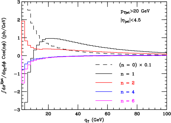
Figure 2: Lowest-order transverse-momentum spectrum $d\sigma_{n}/dq_{T}$ of $cos(n\varphi)$ harmonics in the case of $Z$+jet production.

We consider the $q_{T}$ spectrum $d\sigma_{n}/dq_{T}$ of $\cos(n\varphi)$ harmonics (see Eq. (26)), and in Fig. 2 we present our lowest-order numerical results for $Zj$ production. Note that in Fig. 2 we present the $q_{T}$ dependence of $d\sigma_{n}/dq_{T}$, whereas the azimuthal asymmetries in Fig. 1 are presented as functions of $r_{\rm cut}=q_{\rm cut}/M$ and are obtained by integration of $d\sigma_{n}/dq_{T}$ over $q_{T}$ with the lower limit $q_{T}>q_{\rm cut}$. Note also that we are not showing results for $d\sigma_{n}/dq_{T}^{2}$ (see Eqs. (17) and (26)), which is the $q_{T}$ differential cross section that we typically use throughout the text of this paper. In particular, since $d\sigma_{n}/dq_{T}=2q_{T}d\sigma_{n}/dq_{T}^{2}$, the presence of singular harmonics (with $n=1,2,\dots$) implies that $d\sigma_{n}/dq_{T}\propto 1/q_{T}$ at the lowest perturbative order.

We comment on the results in Fig. 2. As in the case of Fig. 1, in Fig. 2 we also present the result for the harmonic with $n=0$ (i.e., the azimuthally-integrated $q_{T}$ cross section). Since we are considering finite values of $q_{T}$ ($q_{T}>2$ GeV), the plus-prescription (see Eq. (17)) is not effective and the harmonic with $n=0$ has a dominant behaviour that is proportional to $1/q_{T}\ln(M/q_{T})$ at small values of $q_{T}$: the corresponding numerical results in Fig. 2 are consistent with such behaviour. The other results in Fig. 2 regard the $n$-th harmonics with the specific values $n=1,2,4,6$. The numerical results for these azimuthal-correlation harmonics have similar quantitative features: $d\sigma_{n}/dq_{T}$ is small and it has a mild dependence on $q_{T}$ in the region where $q_{T}\raisebox{-2.58334pt}{\hbox to0.0pt{$\,\sim\,$\hss}}\raisebox{1.72218pt}{$\,>\,$}20$ GeV; at smaller values of $q_{T}$, the $q_{T}$ shape changes, and the absolute magnitude of $d\sigma_{n}/dq_{T}$ increases rapidly as $q_{T}$ decreases. This small-$q_{T}$ numerical behaviour is consistent with the dependence $d\sigma_{n}/dq_{T}\propto 1/q_{T}$, and we interpret these results as a clear indication of singular azimuthal harmonics with $n=1,2,4,6$. As we have previously discussed, the harmonic with $n=2$ has singularities of both collinear and soft origins. The initial-state collinear radiation at the point $i)$ cannot give a singular contribution to the harmonic with $n=1,4,6$: in the case of these harmonics the singularity is due to the soft wide-angle radiation at the point $ii)$ (radiation at large angles with respect to the directions of the initial-state colliding partons and to the direction of the momentum of the jet $j$ in the $Zj$ system). If $d\sigma_{n}/dq_{T}\propto 1/q_{T}$ at small values of $q_{T}$, the size of the $q_{T}$ slope of $d\sigma_{n}/dq_{T}$ roughly corresponds to the size of the $n$-th harmonic of the coefficient $a_{\rm corr}({\mbox{\boldmath${\hat{q}}_{T}$}})$ in Eq. (17). From the comparison of the results with $n=1,2,4,6$ in the small-$q_{T}$ region of Fig. 2, we notice that the $q_{T}$ slope of $d\sigma_{n}/dq_{T}$ with $n=1$ is sizeable and this is a clear evidence of singular harmonics with odd values of $n$.

5.2 Resummation

The perturbative resummation of singular azimuthal-correlation contributions was considered in Refs. [11, 12]. Reference [11] presents an all-order treatment (i.e., the treatment is valid to arbitrary logarithmic accuracy) of azimuthal correlations, but it is limited to processes with colourless systems $F$ (the individual particles in $F$ have no QCD colour charge). Therefore, Ref. [11] only deals with azimuthal correlations due to initial-state collinear radiation (see the point $i)$ previously mentioned in Sect. 5.1) for production processes that occur through the gluon fusion channel ($gg\rightarrow F+X$). The all-order resummation for $Q{\bar{Q}}$ production in Ref. [12] is limited to an explicit treatment up to NNLL accuracy, but it deals with a specific example of the relevant case in which the produced final-state system $F$ is colourful (the individual particles in $F$ carry QCD colour charge). Therefore, the analysis and results of Ref. [12] not only deal with collinear radiation, but they also deal with all the main conceptual (and technical) aspects related to azimuthal-correlation effects due to soft wide-angle radiation (see the point $ii)$ previously mentioned in Sect. 5.1). The all-order resummation structure in Ref. [12] is quite different from that of azimuthally-insensitive $q_{T}$ cross sections (e.g., the case of the DY process [28]): the former includes resummation factors and helicity/colour correlations that originate from the collinear/soft contributions at the points $i)$ and $ii)$ in Sect. 5.1. The resummation results of Ref. [12] certainly have some process-dependent features (due to the specific production of $F=\{Q{\bar{Q}}\}$), but they are generalizable (although with specific differences and, possibly, complications at the technical level) to generic production processes of the type in Sect. 4.1 with final-state colourful systems $F$ (e.g., $F=\{Vj\},\{jj\}$). Therefore, we can consider the all-order resummation for $Q{\bar{Q}}$ production in Ref. [12] as the prototype of resummation for this entire class of processes and, consequently, we can present some general comments (by avoiding cumbersome technicalities) in the following.

The all-order resummation in Ref. [12] is performed in $\bf b$ space, by treating azimuthally-independent and azimuthal-correlations contributions on equal footing. Then the $q_{T}$ cross section is obtained by inverse Fourier transformation of the resummed result from $\bf b$ space to $q_{T}$ space. To facilitate the discussion of the comparison (analogies and differences) with the azimuthally-insensitive case (see Sect. 4.2), it is convenient to consider the $q_{T}$ dependence of the $n$-th harmonic:

$$\frac{d\sigma_{n}}{dM^{2}dq_{T}^{2}}\equiv\int_{0}^{2\pi}d\varphi\;\cos(n\varphi)\;\frac{d\sigma}{dM^{2}\,dq_{T}^{2}\,d\varphi}\;\;.$$ (26)

The azimuthal asymmetry in Eq. (11) is obtained by integration of Eq. (26) over $q_{T}$. Considering harmonics, the inverse Fourier transformation from $\bf b$ space to $q_{T}$ space can be recast in the form of a Bessel transformation. In particular, the $n$-th harmonic projects out the $n$th-order Bessel function $J_{n}(x)$ (see, e.g., Sect. 6 in Ref. [11]), and the final result of the resummation procedure of the singular azimuthal-correlation terms has the following (sketchy) form:

$$\frac{d\sigma^{(\rm res)}_{n}}{dM^{2}dq_{T}^{2}}=\int_{0}^{+\infty}db\;b\;J_{n}(bq_{T})\;\Sigma_{n}^{(\rm res)}(M,b)\;\;.$$ (27)

The resummation formula (27) allows us to discuss analogies and differences with respect to the corresponding formula (24) for the azimuthally-independent case (which coincides with the $n=0$ harmonic). Obviously, we can also consider the $n$-th harmonic that is obtained through the replacement $\cos(n\varphi)\rightarrow\sin(n\varphi)$ of the weight function in Eq. (26). Such a replacement does not change the Bessel transformation structure of Eq. (27), although the factor $\Sigma_{n}^{(\rm res)}$ has different explicit expressions for cosine and sine harmonics. The factor $\Sigma_{n}^{(\rm res)}(M,b)$ in Eq. (27) embodies the effect of the all-order resummation procedure in $b$ space. In the following, we first comment on the perturbative expansion of Eq. (27) and, then, we discuss the effect of perturbative resummation.

At the lowest perturbative order, the factor $\Sigma_{n}^{(\rm res)}(M,b)$ in the integrand of Eq. (27) corresponds to the Fourier transformation of the singular contribution $a_{\rm corr}({\mbox{\boldmath${\hat{q}}_{T}$}})/q_{T}^{2}$ in Eq. (17). Therefore, $\Sigma_{n}^{(\rm res)}(M,b)$ is simply proportional to the $n$-th harmonic of the azimuthal function $a_{\rm corr}({\mbox{\boldmath${\hat{q}}_{T}$}})$ and its dependence on $b$ is only due to the Bessel transformation of $1/q_{T}^{2}$. This $b$ dependence is that of the following integral over $q_{T}$:

$${\widehat{I}}^{\;[\,n\,]}_{0}(b)=\int_{0}^{+\infty}\frac{dq_{T}^{2}}{q_{T}^{2}}\;J_{n}(bq_{T})=\frac{2}{n}\;\;,\quad\quad(n=1,2,3\dots)\;\;,$$ (28)

We note that, having selected the $n$-th harmonic, the non-integrable singular function $1/q_{T}^{2}$ has a well defined Bessel transformation. We also note that this Bessel transformation is a constant function of $b$ in the large-$b$ region.

At higher perturbative orders, singular azimuthal correlations produce a dependence of the $q_{T}$ cross section $d\sigma/dM^{2}d^{2}{\mbox{\boldmath$q_{T}$}}$ on $1/q_{T}^{2}$ times powers of $\ln(M^{2}/q_{T}^{2})$ (with at most two powers of $\ln(M^{2}/q_{T}^{2})$ for each additional power of $\alpha_{\mathrm{S}}$). As discussed in Sect. 4.1, such $q_{T}$ dependence is factorized with respect to the dependence on the azimuthal-correlation angle. Therefore, the $b$ dependence of $\Sigma_{n}^{(\rm res)}(M,b)$ is due to the Bessel transformation of these singular functions of $q_{T}$. For example, in the case of the 2nd harmonic the dominant (DL) next-order correction is proportional to the following $q_{T}$ space integral:

$${\widehat{I}}^{\;[\,2\,]}_{2}(M,b)=\int_{0}^{+\infty}\frac{dq_{T}^{2}}{q_{T}^{2}}\;\ln^{2}\!\left(\frac{M^{2}}{q_{T}^{2}}\right)\,J_{2}(bq_{T})=\;\ln^{2}\!\left(\frac{b^{2}M^{2}}{b_{0}^{2}}\right)-2\ln\!\left(\frac{b^{2}M^{2}}{b_{0}^{2}}\right)+2\;\;,$$ (29)

where $b_{0}=2e^{-\gamma_{E}}$ ($\gamma_{E}=0.5772\dots$ is the Euler number) is a numerical coefficient (of kinematical origin) that customarily appears in the context of Fourier (Bessel) transformations of logarithmic functions. In general, the typical singular behaviour of $d\sigma_{n}/dM^{2}dq_{T}^{2}$ at small $q_{T}$ leads to contributions to $\Sigma_{n}^{(\rm res)}(M,b)$ that are proportional to the following basic integrals:

$${\widehat{I}}^{\;[\,n\,]}_{k}(M,b)\equiv\int_{0}^{+\infty}\frac{dq_{T}^{2}}{q_{T}^{2}}\;\ln^{k}\!\left(\frac{M^{2}}{q_{T}^{2}}\right)\,J_{n}(bq_{T})\;\;,\quad\quad(n=1,2,3\dots)\;\;.$$ (30)

The result of the basic integrals is

$${\widehat{I}}^{\;[\,n\,]}_{k}(M,b)=\frac{2}{n}\ln^{k}\!\left(\frac{b^{2}M^{2}}{b_{0}^{2}}\right)+\sum_{m=1}^{k}\frac{k!\;(-1)^{m}}{m!\,(k-m)!}\;{\widehat{d}}^{\;[\,n\,]}_{m}\;\ln^{k-m}\!\left(\frac{b^{2}M^{2}}{b_{0}^{2}}\right)\;,\quad\!\!(k\geq 1,n=1,2,3,\dots)\,,$$ (31)

where ${\widehat{d}}^{\;[\,n\,]}_{m}$ are numerical coefficients that depend on $n$ and $m$ (see Eq. (34)). Note that each of these integrals ${\widehat{I}}^{\;[\,n\,]}_{k}(M,b)$ is a polynomial of degree $k$ in the variable $\ln(bM)$.

We note that the result in Eq. (31) for the integrals ${\widehat{I}}^{\;[\,n\,]}_{k}$ can be obtained by using the generating function method that is used in Appendix B of Ref. [40]. The relevant generating function is

$$\int_{0}^{+\infty}\frac{dq_{T}^{2}}{q_{T}^{2}}\;\left(\frac{q_{T}^{2}}{M^{2}}\right)^{\!\lambda}\;J_{n}(bq_{T})=\;\left(\frac{b_{0}^{2}}{b^{2}M^{2}}\right)^{\!\lambda}\;{\widehat{d}}^{\;[\,n\,]}(\lambda)\;\;,$$ (32)

with

$${\widehat{d}}^{\;[\,n\,]}(\lambda)=\left(\frac{2}{b_{0}}\right)^{\!2\lambda}\;\frac{\Gamma(\lambda+n/2)}{\Gamma(1-\lambda+n/2)}\;\;,$$ (33)

where $\Gamma(z)$ is the Euler Gamma function. In particular, the coefficient ${\widehat{d}}^{\;[\,n\,]}_{m}$ in Eq. (31) is the $m$-th derivative of ${\widehat{d}}^{\;[\,n\,]}(\lambda)$ with respect to $\lambda$ at the point $\lambda=0$:

$${\widehat{d}}^{\;[\,n\,]}_{m}=\left[\left(\frac{d}{d\lambda}\right)^{\!m}\;{\widehat{d}}^{\;[\,n\,]}(\lambda)\right]_{\lambda=0}\;\;.$$ (34)

We remark again that the singular (and non-integrable) azimuthal-correlation contributions in $q_{T}$ space at each f.o. have a corresponding $n$th-order Bessel transformation in $b$ space (see Eqs. (28)–(31)). Since the singular terms have an azimuthal dependence that is factorized with respect to the $q_{T}$ dependence in $q_{T}$ space, our remark equally applies to the two-dimensional Fourier transformation from $q_{T}$ space to ${\bf b}$ space of the entire azimuthal-correlation component $d\sigma^{\rm corr}/dM^{2}d^{2}{\mbox{\boldmath$q_{T}$}}$ of the cross section (the projection onto the $n$-th harmonic in $q_{T}$ space and the sum over an infinite set of harmonics in ${\bf b}$ space are procedures that can be applied with no further conceptual difficulties). The general f.o. structure of $\Sigma_{n}^{(\rm res)}(M,b)$ in the large-$b$ region is formally similar to that of the corresponding function $\Sigma_{\rm az.av.}^{(\rm res)}(M,b)$ for the azimuthally-averaged cross section. In both cases we are dealing with logarithmically-enhanced singular terms in $q_{T}$ space at small values of $q_{T}$ ($q_{T}\ll M$) and with corresponding powers of $\ln(bM)$ and constant terms in $b$ space at large values of $b$ ($bM\gg 1$). In both cases the all-order resummation procedure in $b$ space deals with the resummation of $\ln(bM)$ terms, and the formally dominant contributions at each f.o. are of DL type (two additional powers of $\ln(bM)$ for each additional power of $\alpha_{\mathrm{S}}$). In the case of azimuthal correlations, the $\ln(bM)$ and constant terms originate from the Fourier (Bessel) transformation of non-integrable functions of $q_{T}$ (see Eq. (30)). This origin can be contrasted at the formal level with that of the analogous contributions to the azimuthally-averaged case, in which the $\ln(bM)$ (and constant) terms arise from the Fourier (Bessel) transformation of terms that are plus-distributions (and $\delta$-function contributions) of $q_{T}$. The basic integrals that occur in the azimuthally-averaged case are obtained from the right-hand side of Eq. (30) throughout the replacement $J_{n}\rightarrow J_{0}$ and the replacement of the $q_{T}$ functions with the corresponding plus-distributions. The explicit computation of these integrals for the azimuthally-averaged case is presented in the Appendix B of Ref. [40] (see, in particular, Eqs. (129) and (141) of the arXiv version of Ref. [40] or, equivalently, Eqs. (B.18) and (B.30) of the corresponding published version).

We now discuss the all-order behaviour of the resummed result in Eq. (27). The $b$-space resummed cross section $\Sigma_{n}^{(\rm res)}$ involves several factors (see Sect. 6 in Ref. [11] and Sect. 2 in Ref. [12]) and, in particular, the explicit dependence on the $n$-th harmonic is definitely related to the specific multiparticle system $F$ that is produced in the hard-scattering process. Although the resummed functions $\Sigma_{\rm az.av.}^{(\rm res)}$ and $\Sigma_{n}^{(\rm res)}$ in Eqs. (24) and (27) are different, the analysis in Refs. [11, 12] shows that the dominant DL behaviour of these two $b$-space cross sections is controlled by the same universal (process-independent) factor, namely, the Sudakov form factor $S_{c}(M,b)$ that we have already recalled in Sect. 4.2. The presence and universality of this common factor, $S_{c}(M,b)$, in the resummed result of both cross sections in Eqs. (24) and (27) follow from the physical origin of the DL contributions to both cross sections: the DL terms originate from radiated partons that are soft and collinear to the initial-state colliding partons $c_{1}$ and $c_{2}$ of the corresponding main production channels (see Eq. (15)) in the small-$q_{T}$ region.

As in the case of azimuthally-independent contributions (see our comments in Sect. 4.2), the Sudakov form factor produces a strong suppression of the large-$b$ region ($bM\gg 1$) in the integrand on the right-hand side of Eq. (27). This damping effect leads to resummed perturbative predictions for the $q_{T}$ dependence of the $n$-th azimuthal harmonic $d\sigma_{n}/dM^{2}dq_{T}^{2}$ that have a smooth and, especially, integrable behaviour in the small-$q_{T}$ region. The integrable behaviour can be checked by performing the limit $q_{T}\rightarrow 0$ of Eq. (27). Owing to the Sudakov-type suppression of the large-$b$ integration region, we can proceed (as in Sect. 4.2) to use the small-$q_{T}$ approximation $J_{n}(bq_{T})={\cal O}((bq_{T})^{n})$ in the right-hand side of Eq. (27), and we obtain [11]

$$\frac{d\sigma^{(\rm res)}_{n}}{dM^{2}dq_{T}^{2}}\propto q_{T}^{n}\;\;\quad\quad\quad(q_{T}\rightarrow 0)\;\;.$$ (35)

The small-$q_{T}$ behaviour in Eq. (35) is integrable at $q_{T}=0$ for every harmonic $(n=1,2,3,\dots)$. This is a highly non-trivial result of the all-order resummation procedure of terms that individually behave in a very singular way as $1/q_{T}^{2}$ (modulo powers of $\ln(M^{2}/q_{T}^{2}$)). In the case of the azimuthally-averaged cross section, as the result of the resummation procedure, the fixed-order singular behaviour is turned into the constant behaviour of Eq. (25). In the case of the $n$-th azimuthal harmonic the effect of resummation is even more substantial, since the $1/q_{T}^{2}$ singular behaviour is turned into the suppressed power-like behaviour, $q_{T}^{n}$, of Eq. (35). We thus expect that the shape of the resummed $q_{T}$ spectrum, $d\sigma_{n}/dM^{2}dq_{T}^{2}$, for the $n$-th azimuthal harmonic can be substantially different from the shape of the $q_{T}$ spectrum for the azimuthally-averaged cross section. Independently of the detailed $q_{T}$ shape, the all-order perturbative resummation has a ‘dramatic’ effect on the total production rate of the azimuthal asymmetries. The total ($q_{T}$ integrated) azimuthal asymmetries turn out to be finite (and computable) after resummation, whereas they can be divergent at fixed perturbative orders. In contrast, the total ($q_{T}$ integrated) azimuthally-averaged cross section is finite order-by-order in perturbation theory, and it is basically not affected by resummation effects in the small-$q_{T}$ region.

As we have discussed in Sect. 4.1, the f.o. divergences of azimuthal asymmetries are produced by primary real emission of one final-state parton, which is absolutely not compensated by virtual radiation at the corresponding perturbative order. At higher perturbative orders, real emission (which is strictly necessary to produce azimuthal asymmetries) is accompanied by ensuing virtual and real radiative effects. Throughout all-order resummation, virtual radiative effects turn out to be dominant in the small-$q_{T}$ region, and they produce the Sudakov form factor suppression that makes the azimuthal asymmetries finite (and with a smooth $q_{T}$ shape at small values of $q_{T}$).

The small-$q_{T}$ behaviour in Eqs. (25) and (35) is the result of a combined effect of QCD dynamics and kinematics. We conclude this subsection with a brief discussion of this statement.

We note that the $q_{T}$ dependence in Eqs. (25) and (35) is eventually driven by the corresponding small-$q_{T}$ behaviour of the Bessel functions $J_{n}(bq_{T})$ in the right-hand side of Eqs. (24) and (27). The presence of the Bessel function $J_{n}$ in Eqs. (24) and (27) has a kinematical origin: the Bessel functions simply arise from the two-dimensional Fourier transformation from $\bf b$ space to $q_{T}$ space after projection onto the $n$-th harmonic component. This kinematical origin, however, does not imply that the small-$q_{T}$ behaviour in Eqs. (25) and (35) is purely produced by (all-order) kinematical effects. Such small-$q_{T}$ behaviour has indeed a dynamical origin, since it is due to the strong Sudakov-type suppression of the large-$b$ integration region (see Eqs. (24) and (27)) that is embodied in the resummed components $\Sigma_{\rm az.av.}^{(\rm res)}$ and $\Sigma_{n}^{(\rm res)}$. To make clear the role of this strong suppression, we can consider an explicit counterexample as given by a $b$ space function $\Sigma_{n}(M,b)$ that is is power-like suppressed by the factor $(1/bM)^{2\lambda}$ in the large-$b$ region (we assume that $\lambda$ is positive, and we may also assume that $\lambda$ is arbitrarily large if we want to obtain a suppression effect that is quantitatively strong). The Bessel transformation (see the right-hand side of Eq. (27)) of such a power-like function leads to a $q_{T}$ differential cross section $d\sigma_{n}/dM^{2}dq_{T}^{2}$ that is equally power-like suppressed as $(q_{T}^{2})^{\lambda-1}$ in the small-$q_{T}$ region, with no power-like dependence on the order $n$ of the Bessel function $J_{n}$. The Sudakov-type suppression in $b$ space acts differently on the azimuthally-averaged cross section and on the azimuthal asymmetries in $q_{T}$ space. In the case of the azimuthally-averaged cross section $d\sigma_{\rm az.av.}^{({\rm res})}/dM^{2}dq_{T}^{2}$, resummation leads to a smearing of the LO $\delta$-function behaviour (see Eq. (16)), and the resummed $q_{T}$ distribution broadens at small values of $q_{T}$. In the case of the azimuthal asymmetry $d\sigma_{n}^{({\rm res})}/dM^{2}dq_{T}^{2}$, resummation leads to a suppression of the $1/q_{T}^{2}$ behaviour at the lowest order, and the resummed $q_{T}$ distribution is power-like suppressed at small values of $q_{T}$. In both cases, all-order kinematical effects have a non-negligible role. Transverse-momentum conservation, which is ‘exactly’ (provided $q_{T}\ll M$) implemented through $b$ space resummation, is eventually responsible for the small-$q_{T}$ behaviour in Eqs. (24) and (27), which is not a DL exponentially suppressed $q_{T}$ behaviour. This feature is (partly) a consequence of the two-dimensional nature of the kinematical conservation law of the transverse-momentum vector $q_{T}$, which is the relevant kinematical variable for the small-$q_{T}$ behaviour of the azimuthally-averaged cross section and of the azimuthal asymmetries. In contrast, we can recall the effect of resummation on observables, such as event shapes, that are controlled by kinematical variables (e.g., energies and invariant masses) with one-dimensional conservation laws: near the exclusive boundary of the phase space, these observables have a DL exponential suppression (see, e.g., Ref. [41]), a suppression effect that is stronger than that produced by any fixed power of the kinematical distance from the phase space boundary.

As we have discussed in Sect. 3, QED radiative corrections can also produce singular azimuthal asymmetries (for instance, in the DY process $q{\bar{q}}\rightarrow Z(e^{+}e^{-})+X$). The QCD resummation procedure that we have discussed in this subsection can equally be applied to QED radiative corrections, and it conceptually leads to the same results and resummation effects that we have just discussed for the QCD case. The same reasoning and conclusions are basically valid in a pure QED context, such as, for instance, in the QED computation of $e^{+}e^{-}\rightarrow\mu^{+}\mu^{-}+X$ (although the resummed $b$-space expression and the QED Sudakov form factor acquire an explicit dependence on the mass of the colliding leptons in the initial state).

5.3 Azimuthal asymmetries in $t{\bar{t}}$ production

To illustrate resummed results on the $q_{T}$ dependence of azimuthal asymmetries at the quantitative level, we choose the specific process of $t{\bar{t}}$ production. Our choice has several reasons, besides the fact that $t{\bar{t}}$ production is certainly a process of high phenomenological relevance. One reason is that for $t{\bar{t}}$ production we have explicit theoretical control [12] of singular azimuthal correlations and their QCD resummation. Moreover, due to the non-vanishing QCD colour charge of the produced $t$ and ${\bar{t}}$, in this process we are dealing with singular azimuthal-correlation effects of both collinear and soft origin (see the points $i)$ and $ii)$ in Sect. 5.1). These effects appear in the QCD radiative corrections to both production channels of quark-antiquark annihilation ($q{\bar{q}}\rightarrow t{\bar{t}}+X$) and gluon fusion ($gg\rightarrow t{\bar{t}}+X$). Finally, singular azimuthal correlations first arise at the NLO level with respect to the computation of the $t{\bar{t}}$ total cross section and, therefore, they are expected to produce effects that have a relatively-large size.

Perturbative resummation of singular azimuthal correlations is under theoretical control [11] also in the case of production processes of colourless systems $F$ (e.g., $F\!=\{\gamma\gamma\}$, $\{Z\gamma\}$, $\{ZZ\}$, $\{W^{+}W^{-}\}$). However, in these cases we are sensitive only to singular contributions of collinear origin (see the point $i)$ in Sect. 5.1) and not to those of soft origin (see the point $ii)$ in Sect. 5.1). These singular contributions of collinear origin arise only from QCD radiative corrections to the sole gluon fusion production channel $gg\rightarrow F+X$. The colourless system $F$ is typically produced at the LO throughout the quark-antiquark production channel ($q{\bar{q}}\rightarrow F$). Owing to the absence of direct coupling of the gluons to the colourless particles in $F$, the production channel $gg\rightarrow F$ is suppressed by some powers of $\alpha_{\mathrm{S}}$ with respect to the channel $q{\bar{q}}\rightarrow F$: typically, $gg\rightarrow F$ enters at the NNLO in the computation of the total cross section, and the singular azimuthal asymmetries due to $gg\rightarrow F+X$ first appear at the N³LO. Therefore, there is a formal mismatch (suppression) of two powers of $\alpha_{\mathrm{S}}$ of the expected relative size of singular azimuthal-correlation effects (which turn out to be finite after QCD resummation) in going from $t{\bar{t}}$ production to the production of a colourless system $F$. Owing to all the reasons that we have just discussed, we think it is more ‘interesting’ to focus our illustrative quantitative analysis on the case of $t{\bar{t}}$ production.

We consider $t{\bar{t}}$ production in $pp$ collisions with the centre–of–mass energy ${\sqrt{s}}=8$ TeV at the LHC. In Sect. 3 (see Fig. 1-right) we have considered the computation of $\cos(n\varphi)$ harmonics, where $\varphi$ is the azimuthal angle of the top quark in the CS frame (the differential cross section is integrated over the polar angle of the top quark and over the rapidity $y$ and invariant mass $M$ of the $t{\bar{t}}$ pair). The $n$-th harmonics in Fig. 1-right are integrated over the transverse momentum $q_{T}$ of the $t{\bar{t}}$ pair (with the lower limit $q_{T}>q_{\rm cut}$). In this subsection we present numerical results on the $q_{T}$ dependence of the $n$-th harmonic, and we explicitly consider $d\sigma_{n}/dq_{T}$ rather than $d\sigma_{n}/dq_{T}^{2}$. Since $d\sigma_{n}/dq_{T}=2q_{T}d\sigma_{n}/dq_{T}^{2}$, the presence of singular harmonics implies that $d\sigma_{n}/dq_{T}\propto 1/q_{T}$ (modulo logs) as $q_{T}\rightarrow 0$ in f.o. perturbative calculations.

We specifically consider the $\cos(2\varphi)$ harmonic. We present results at the lowest perturbative order (Fig. 3-left) and including all-order resummation (Fig. 3-right).

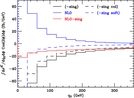
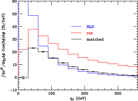
Figure 3: Transverse-momentum spectrum $d\sigma_{n}/dq_{T}$ for the $n=2$ harmonic in $t\bar{t}$ production. In the left panel the exact NLO result (blue) is compared to the $1/q_{T}^{2}$ singular component (black), which is split in its collinear (black dashed) and soft (blue dashed) parts. The singular components are plotted with opposite overall sign. The finite result (NLO-sing) that is obtained by subtracting the singular component from the exact NLO result is also shown (red). In the right panel the NLO result (blue) is compared to the purely resummed result (red) and to the complete matched result (black), computed as described in the text.

The set-up and parameters of the lowest-order calculation are the same as those described and used in Sect. 3. Specifically, we compute the NLO contribution to $t{\bar{t}}$ production that is due to all tree-level partonic processes whose final state is ‘$t{\bar{t}}+1$ parton’. The result of the $q_{T}$ dependence of the $\cos(2\varphi)$ asymmetry at NLO is shown in Fig. 3-left: the cross section increases by decreasing $q_{T}$ and, in the small-$q_{T}$ region, the increasing behaviour is consistent with the $1/q_{T}$ behaviour predicted in Ref. [12]. The NLO result in the first $q_{T}$-bin (which includes the region where $q_{T}=0$) is not shown in Fig. 3-left since it would be divergent to $+\infty$. The singular $1/q_{T}$ behaviour predicted in Ref. [12] in analytic form can be evaluated numerically, and the corresponding result is also presented in Fig. 3-left. Actually, in Fig. 3-left we plot the NLO singular result with the opposite overall sign (we do that for better visibility, since this avoids the presentation of close histograms). We remark that the NLO singular result in Fig. 3-left exactly behaves as $1/q_{T}$ (i.e., it corresponds to the 2nd harmonic of the term $a_{\rm corr}({\mbox{\boldmath${\hat{q}}_{T}$}})/q_{T}^{2}$ in Eq. (17)), with no additional $q_{T}$ dependence due to NLO contributions that are non-singular in the limit $q_{T}\rightarrow 0$ (i.e., the terms denoted by dots in the right-hand side of Eq. (17)). In Fig. 3-left we also present the numerical result (it is denoted by the label ‘NLO $-$ sing’) that is obtained by subtracting the $1/q_{T}$ singular part from the complete NLO result. Therefore, ‘NLO $-$ sing’ is expected (predicted) [12] to be finite in the limit $q_{T}\rightarrow 0$ and, moreover, from it we can numerically extract the behaviour of the dominant non-singular contribution to the NLO asymmetry in the small-$q_{T}$ region. By direct inspection of Fig. 3-left we see that ‘NLO $-$ sing’ is indeed finite: in the limit $q_{T}\rightarrow 0$ the finite result appears to be numerically consistent with a non-vanishing (actually, negative) constant value. This implies that, in the case of the $\cos(2\varphi)$ asymmetry, the dominant non-singular behaviour of $d\sigma_{n}/dq_{T}$ is proportional to a constant.

As we have discussed, singular azimuthal correlations can have collinear and soft origins (see the points $i)$ and $ii)$ in Sect. 5.1). In the case of $t{\bar{t}}$ production, the collinear and soft contributions were separately evaluated in Ref. [12]. In Fig. 3-left we report the numerical results of the splitting of the complete NLO singular contribution in its collinear and soft parts. We note that the collinear and soft parts have the same relative sign, so that there is no numerical compensation between them. Both the collinear and soft parts behave as $1/q_{T}$: removing one of these two parts from the singular contribution would lead to a divergent result for the combination ‘NLO $-$ sing’ in the limit $q_{T}\rightarrow 0$. The overall size of the soft part is smaller than that of the collinear part, however, the soft part is definitely not negligible: the ratio between the soft and collinear parts is approximately 0.3. Moreover, we remark that the relative size of collinear and soft contributions depends on the type of colliding hadrons and on the centre–of–mass energy of the collision.

We also comment on the results of Fig. 3-left in the large-$q_{T}$ region. We note that ‘NLO $-$ sing’ is negative, and this is what we can generally expect at sufficiently large values of $q_{T}$. The NLO calculation is expected to be physically well behaved at large $q_{T}$ and, hence, the NLO result should be suppressed stronger than $1/q_{T}$. On the contrary, according to our definition, the small-$q_{T}$ singular approximation behaves exactly as $1/q_{T}$ over the entire $q_{T}$ range. As a consequence, at large values of $q_{T}$ the singular approximation overshoots the NLO result, and the result of ‘NLO $-$ sing’ turns out to be negative.

We now move to consider resummation for the $q_{T}$ dependence of the $\cos(2\varphi)$ asymmetry. Our quantitative results are presented in Fig. 3-right. Before discussing the results in Fig. 3-right, we briefly comment on the actual content of our resummed calculation. Details on the calculation will be presented in a forthcoming paper, in which we also consider resummation results for the customary azimuthally-integrated $q_{T}$ cross section in $t{\bar{t}}$ production.

We use the resummed theoretical results of Ref. [12] for $t{\bar{t}}$ production by applying the implementation formalism of Ref. [40]. This formalism has so far been applied to transverse-momentum resummation of azimuthally-integrated (or azimuthally-insensitive) cross sections for many production processes (see, e.g., Ref. [44] and related references therein). The complete result $d\sigma$ for the azimuthal-correlation component of the $q_{T}$ differential cross section is obtained by using a matching procedure that combines the resummation of the singular contributions ($d\sigma^{(\rm res)}$) with the evaluation of non-singular (finite) contributions ($d\sigma^{(\rm fin)}$) at a given f.o. in perturbation theory. We write $d\sigma=d\sigma^{(\rm res)}+d\sigma^{(\rm fin)}$, and we work at NLL+NLO accuracy for the resummed (NLL) and f.o. (NLO) contributions. Therefore, the f.o. part $d\sigma^{(\rm fin)}$ that contributes to the complete matched (res + fin) result $d\sigma$ in Fig. 3-right is exactly the ‘NLO $-$ sing’ contribution in Fig. 3-left. The resummed part $d\sigma^{(\rm res)}$ is first computed in $b$ space, where we are dealing with the resummed factor $\Sigma^{(\rm res)}(M,{\bf b})$. The resummed factor $\Sigma^{(\rm res)}(M,{\bf b})$ is proportional to the contribution from the singular part of the NLO result (see Fig. 3-left) and, very roughly speaking, it is multiplied by a form factor $\exp\{{\cal G}(M,b)\}$ that is evaluated in resummed form up to NLL accuracy. We mean that in the large-$b$ region ($bM\gg 1$) we have ${\cal G}(M,b)={\cal G}^{LL}(M,b)+{\cal G}^{NLL}(M,b)$, where ${\cal G}^{LL}(M,b)$ and ${\cal G}^{NLL}(M,b)$ embody the resummation ($\sum_{k=1}^{\infty}$) of the LL terms $\alpha_{\mathrm{S}}^{k}\ln^{k+1}(bM)$ and the NLL terms $\alpha_{\mathrm{S}}^{k}\ln^{k}(bM)$, respectively. We remark an important difference between ${\cal G}^{LL}$ and ${\cal G}^{NLL}$. The LL contribution ${\cal G}^{LL}(M,b)$ is essentially process independent and it basically depends on the initial-state colliding partons of the partonic subprocesses $gg\rightarrow t{\bar{t}}+X$ and $q{\bar{q}}\rightarrow t{\bar{t}}+X$. By contrast, ${\cal G}^{NLL}(M,b)$ includes an important amount of process-dependent information. In particular, it includes the effect of soft wide-angle radiation for the $t{\bar{t}}$ production process. This effect is controlled by a colour-dependent anomalous dimension, namely, the soft anomalous dimension $\bf\Gamma^{(1)}_{t}$ in Ref. [12] (see Eqs. (16), (17) and (33) in Ref. [12]), and we resummed the effect in complete exponentiated form throughout the diagonalization of $\bf\Gamma^{(1)}_{t}$ in colour space.

At the technical level, we note that we compute $\Sigma^{(\rm res)}(M,{\bf b})$ in two-dimensional ${\bf b}$ space and we obtain the $q_{T}$ cross section by numerically performing the Fourier transformation to $q_{T}$ space. The computation of the $\cos(n\varphi)$ harmonic is also performed by numerically integrating over $\varphi$. Therefore, we do not perform the projection onto the $n$-th harmonic in analytic form (see Eq. (27)), and our implementation can be directly applied to the numerical evaluation of $n$-th harmonics with different values of $n$.

Our quantitative resummed results on the $q_{T}$ dependence, $d\sigma/dq_{T}$, of the $\cos(2\varphi)$ harmonic are presented in Fig. 3-right. We show the purely resummed result ($d\sigma^{(\rm res)}$) and the complete final result after the inclusion of the matching term ($d\sigma^{(\rm fin)}$) at NLO. In Fig. 3-right we also report the NLO result (see Fig. 3-left) for direct comparison with the resummed results. The error bars in the complete matched result denote the numerical errors of our calculation (for simplicity of presentation the numerical error bars are not reported in the other histograms of Fig. 3). By direct inspection, we observe that the purely resummed result quantitatively differs from the complete matched result, and we comment about that below. Since we are considering the results after integration over the invariant mass $M$ of the $t{\bar{t}}$ pair, the characteristic hard scale of the $q_{T}$ cross section is of the order of $2m_{t}$ ($m_{t}$ is the mass of the top quark), which is the minimum value of $M$, and the $q_{T}$ range that is shown in Fig. 3-right includes the regions of small and intermediate values of $q_{T}$. The high-$q_{T}$ region, $q_{T}\raisebox{-2.58334pt}{\hbox to0.0pt{$\,\sim\,$\hss}}\raisebox{1.72218pt}{$\,>\,$}2m_{t}$, is not shown in Fig. 3-right.

We first comment on the results in the large-$q_{T}$ region of Fig. 3-right. We observe that, starting from intermediate values of $q_{T}$ (e.g., $q_{T}\raisebox{-2.58334pt}{\hbox to0.0pt{$\,\sim\,$\hss}}\raisebox{1.72218pt}{$\,>\,$}150$ GeV), the complete resummed result tends to nicely agree with the NLO result. Note that we are not using a direct (though, possibly smooth) switching procedure from the purely resummed result to the NLO result at some intermediate value of $q_{T}$. The agreement between the complete result and the NLO result at large $q_{T}$ is thus a non-trivial consequence of the matching procedure. In the absence of the contribution from the matching term ($d\sigma^{(\rm fin)}$), the purely resummed result sizeably overshoots the NLO result at intermediate and large values of $q_{T}$ (for instance, at $q_{T}\sim 350$ GeV the purely resummed result is about 8 times larger than the NLO result). This feature is due to the fact that the size of $d\sigma^{(\rm res)}$ is driven by the small-$q_{T}$ singular part of the NLO calculation, and the singular part is not a good quantitative approximation of the NLO calculation at intermediate and large values of $q_{T}$ (we have already discussed that and the corresponding overshooting effect in our comments about Fig. 3-left). In the complete (matched) result, the effect of this approximation is compensated by adding $d\sigma^{(\rm fin)}$ (i.e., the ‘NLO $-$ sing’ result of Fig. 3-left), which sizeably decreases $d\sigma^{(\rm res)}$ at large $q_{T}$. Once $d\sigma^{(\rm res)}$ and $d\sigma^{(\rm fin)}$ are combined, the difference between the resummed and NLO results is much reduced at intermediate values of $q_{T}$, and the higher-order (i.e., beyond NLO) resummation terms that are included in our resummed calculation do not have a large residual effect in that $q_{T}$ region.

We now comment on the results in the small-$q_{T}$ region of Fig. 3-right. In this region the resummed results unavoidably differ from the NLO result: the NLO result is much larger at small values of $q_{T}$, and it diverges to $+\infty$ if $q_{T}\rightarrow 0$. According to our previous discussion (see Eq. (35)), the purely resummed result behaves as $d\sigma/dq_{T}\sim q_{T}^{3}$ in the limit $q_{T}\rightarrow 0$, and the numerical results in Fig. 3-right are consistent with this expectation. The maximum value of the resummed cross section is in the region ($q_{T}$ bin) where 30 GeV$<q_{T}<$60 GeV. Using our implementation of the theoretical results of Ref. [12], we have performed a corresponding resummed calculation of the customary (azimuthally-integrated) $q_{T}$ cross section $d\sigma/dq_{T}$ of the $t{\bar{t}}$ pair and we find [46] that its $q_{T}$ shape is quite different from that of the $\cos(2\varphi)$ harmonic in Fig. 3-right (as expected from the general comments below Eq. (35)): $d\sigma_{\rm az.av.}/dq_{T}$ has a maximum at $q_{T}\sim 15$ GeV and a much softer $q_{T}$ spectrum in the small-$q_{T}$ region. The qualitative features of the complete result for the 2nd harmonic are similar to those of the corresponding purely resummed result. However, the inclusion of the non-singular NLO contribution ($d\sigma^{(\rm fin)}$) has a relevant quantitative effect, not only at intermediate values of $q_{T}$ (as previously discussed) but also in the small-$q_{T}$ region (for instance, in the $q_{T}$ bin where 30 GeV$<q_{T}<$60 GeV, the purely resummed result turns out to be reduced by about 40%). We have also checked the quantitative effect of the NLL resummation terms that are due to the inclusion of the soft anomalous dimension $\bf\Gamma^{(1)}_{t}$. We find that also $\bf\Gamma^{(1)}_{t}$ has a substantial effect in the small-$q_{T}$ region: $d\sigma/dq_{T}$ would be quantitatively smaller and with a harder $q_{T}$ shape by removing the effect of $\bf\Gamma^{(1)}_{t}$ (i.e., by simply setting ${\bf\Gamma^{(1)}_{t}}=0$).

By integrating $d\sigma/dq_{T}$ for the $\cos(2\varphi)$ harmonic over the entire kinematical region of $q_{T}$, we find the total value $\sigma_{t{\bar{t}},n=2}=3.0$ pb. In comparison, the value of the $t{\bar{t}}$ total cross section ($\sigma_{t{\bar{t}}}^{NLO}=226$ pb) is about 70 times larger than $\sigma_{t{\bar{t}},n=2}$. We remark that our quantitative results for $\sigma_{t{\bar{t}},n=2}$ and also for the $q_{T}$ dependence of the $\cos(2\varphi)$ harmonic have to be regarded as ‘effective’ lowest-order predictions within (resummed) perturbative QCD. We do not attempt to quantify the theoretical accuracy of these predictions. As is well known, customary procedures (e.g., studies of dependence on factorization and renormalization scales) that can be applied to estimate theoretical uncertainties of lowest-order predictions typically fail in reproducing the quantitative effect of higher-order contributions (this is especially true in the case of QCD calculations for hard-scattering processes in hadron collisions at high energies). A first quantitative estimate of the theoretical uncertainty of the lowest-order predictions requires a computation at the subsequent perturbative order. Once the results at two subsequent orders are known, their relative difference can be used for a quantitative estimate of the theoretical uncertainty. At the present lowest-order level, we limit ourselves to adding few comments. The bulk of the contribution to the $\cos(2\varphi)$ harmonic originates from the small and intermediate regions of $q_{T}$; we find that the high-$q_{T}$ region (say, $q_{T}\raisebox{-2.58334pt}{\hbox to0.0pt{$\,\sim\,$\hss}}\raisebox{1.72218pt}{$\,>\,$}2m_{t}$) gives only a few percent contribution to the total value of $\sigma_{t{\bar{t}},n=2}$. The NLL resummed contributions due to the soft anomalous dimension $\bf\Gamma^{(1)}_{t}$ are not negligible: removing the effect due to $\bf\Gamma^{(1)}_{t}$ in our calculation, we find that the total value of $\sigma_{t{\bar{t}},n=2}$ decreases by about 30%. The total value of $\sigma_{t{\bar{t}},n=2}$ would be much larger by considering the purely resummed term ($d\sigma^{(\rm res)}$) and no matching with the complete NLO calculation: removing the matching contribution ($d\sigma^{(\rm fin)}$), the value of $\sigma_{t{\bar{t}},n=2}$ would increase by roughly a factor of two. This highlights the importance of non-singular NLO effects at small and intermediate values of $q_{T}$.

In our resummed calculation we numerically perform the Fourier transformation from $\bf b$-space to $q_{T}$-space, and we obtain the $q_{T}$ cross section $d\sigma/dq_{T}^{2}d\varphi$. We can then numerically evaluate different harmonics. We have carried out an exploratory numerical computation of the $\cos(4\varphi)$ asymmetry for $t{\bar{t}}$ production, and we find results with the expected features, analogously to the $\cos(2\varphi)$ asymmetry. Nonetheless, the size of the $\cos(4\varphi)$ asymmetry is very small and we do not present corresponding resummed results. As shown in Fig. 1-right, the $n=1$ azimuthal asymmetry for $t{\bar{t}}$ production is not divergent if computed at its lowest perturbative order, and the corresponding $q_{T}$ spectrum is not singular. In view of our discussion in Sect. 5.1, the next-order QCD correction to the $n=1$ harmonic can produce a singular $q_{T}$ spectrum, so that the corresponding QCD prediction can require a resummed calculation at a subdominant logarithmic accuracy with respect to that considered in Ref. [12].

We add some general comments on the contribution of non-singular terms (e.g., the terms denoted by dots in the right-hand side of Eq. (17)) to azimuthal correlations at low values of $q_{T}$. In the case of the azimuthally-averaged cross section $d\sigma_{\rm az.av.}/dq_{T}^{2}$, the perturbative resummation of singular terms produces a constant behaviour in the small-$q_{T}$ region (see Eq. (25)) and, typically (e.g., in absence of additional kinematical cuts), the non-singular terms also have a constant behaviour at low values of $q_{T}$ (order-by-order in the perturbative expansion the ratio between non-singular and singular terms if formally of ${\cal O}(q_{T}^{2}/M^{2})$, modulo logarithms, in the limit $q_{T}\rightarrow 0$). As a consequence, resummed and f.o. non-singular contributions to $d\sigma_{\rm az.av.}/dq_{T}^{2}$ behave similarly at low values of $q_{T}$, although the non-singular contributions are perturbatively (and quantitatively) suppressed. In the case of the cross section $d\sigma_{n}/dq_{T}^{2}$ for the $n$-th harmonic, the resummation of the singular terms produces an enhanced power suppression ($\propto q_{T}^{n}$) of dynamical origin (see Eq. (35)) in the small-$q_{T}$ region and, therefore, non-singular terms are eventually more relevant at low values of $q_{T}$ if they are treated at f.o. in perturbation theory. We note that this reasoning neglects the fact that non-singular terms can also have logarithmic enhancement (powers of $\ln(M/q_{T})$) order-by-order in perturbation theory and, consequently, an appropriate resummation treatment of non-singular terms can be required. For instance, QCD resummation of non-singular terms has been investigated (see Ref. [47] and references therein) for the DY process. Note, however, that non-singular corrections to singular azimuthal correlations are quite different from azimuthal-correlation effects in the DY process and they are expected to have a high degree of process dependence. We also recall that the non-singular terms produce azimuthal-correlation effects whose actual size and $q_{T}$ behaviour depend on the specific definition of the azimuthal-correlation angles (see Eq. (8) and related comments in Sect. 2). In particular, the $q_{T}$ dependence of non-singular terms can be redistributed among different $n$-th harmonics by considering azimuthal correlations that refer to different specifications of the azimuthal angle.

As for non-singular terms, at present we do not have a detailed theoretical understanding that goes beyond their treatment at f.o. . A better understanding of non-singular terms is certainly relevant to have an accurate quantitative control on the detailed $q_{T}$ shape of azimuthal correlations in the region of very-low values of $q_{T}$. We note, however, that non-singular terms have a relatively-mild effect on $q_{T}$ integrated azimuthal correlations. For instance, since non-singular terms are integrable in the limit $q_{T}\rightarrow 0$, their perturbative logarithmic enhancement still gives contributions to the total ($q_{T}$ integrated) harmonic that are parametrically controlled by powers of $\alpha_{\mathrm{S}}$. Moreover, after resummation of the singular terms (and, basically, as a consequence of the behaviour in Eq. (35)), the bulk of the contribution to $d\sigma_{n}/dq_{T}^{2}$ is located at relatively-large values of $q_{T}$ (the bulk of the contribution to $d\sigma_{\rm az.av.}/dq_{T}^{2}$ is typically located at smaller values of $q_{T}$) and, also in this region the logarithmic enhancement of non-singular terms is expected to produce relatively-mild effects (approximately, also these effects are parametrically controlled by powers of $\alpha_{\mathrm{S}}$). In summary, we think that an improved (beyond f.o. perturbation theory) treatment of non-singular terms is relevant especially to determine the detailed (point-by point) $q_{T}$ shape of $d\sigma_{n}/dq_{T}^{2}$ at low values of $q_{T}$, while even the total effect of non-singular terms in the low-$q_{T}$ region (e.g., in the lower $q_{T}$-bin, $q_{T}<30$ GeV, of Fig. 3) can be relatively well under control within a f.o. treatment.

We note that, at very low values of $q_{T}$, also non-perturbative QCD effects can be relevant. In the case of the resummed contribution to the $q_{T}$ cross section, a customary (though much simplified) procedure to model non-perturbative effects consists in supplementing the Sudakov form factor with a non-perturbative form factor that mostly contributes at large values of $b$ in the $b$-space resummation formula (see Eq. (24)). A typical parametrization of the non-perturbative form factor is $e^{-g\,b^{2}}$ ($g$ being a parameter whose size, $g\sim{\cal O}(1\!~{}{\rm GeV}^{2})$, is determined by effects at non-perturbative scales), and it produces a strong damping effect a very large values of $b$. In the resummation formula these non-perturbative effects act in a $b$-region that is already strongly suppressed by the Sudakov form factor and, consequently (after Bessel transformation from $b$ space to $q_{T}$ space), they mainly affect only the region of low values of $q_{T}$ [25, 37]. Such a model of non-perturbative effects can also be applied to the resummed contribution to the $n$-th harmonic (see Eq. (27)), and the non-perturbative parameter can also depend on the harmonic (e.g., $g\rightarrow g_{n}$). We may try to apply a related model also to non-singular terms. We consider (part of) non-singular terms of the $n$-th harmonic, we transform them to $b$-space and then we supplement them with a non-perturbative form factor $e^{-g_{n}\,b^{2}}$. The non-singular terms in $b$-space are power-suppressed at large values of $b$, so that the non-perturbative form factor still acts on a $b$-region that is dynamically suppressed (correspondingly, the non-perturbative form factor mainly affects the region of low values of $q_{T}$). Nonetheless, at very large values of $b$, the exponential suppression that is produced by the non-perturbative form factor is so strong that, in the limit $q_{T}\rightarrow 0$, $d\sigma_{n}/dq_{T}^{2}$ behaves as $q_{T}^{n}$, and the non-singular terms (those that are treated in this way) eventually produce the same $q_{T}$ behaviour as the resummed contribution to $d\sigma_{n}/dq_{T}^{2}$. We cannot argue that such a model is physically justified (such a non-perturbative treatment of non-singular terms is certainly not applicable to azimuthal correlations in a pure QED context). We have mentioned it only to notice that in the region of low values of $q_{T}$ non-singular terms can be affected by both perturbative logarithmic enhancement and non-perturbative contributions. A study of non-perturbative effects in azimuthal-correlation cross sections is definitely beyond the scope of this paper.

6 Summary

In this paper we have considered high-mass systems formed by two or more particles that are produced in hadron collisions, and we have discussed the azimuthal correlations between the system and one of its particles. We refer to particles in an extended sense, namely, pointlike particles and QCD jets. Our main findings can be summarized as follows.

Despite the infrared-safe nature of the azimuthal distribution, the f.o. QCD computation of this observable can be divergent starting from some perturbative order. This conclusion holds for a large class of processes, including $t\bar{t}$, $Vj$, $jj$, $\gamma\gamma$, $ZZ$, $W^{+}W^{-}$ production, while the corresponding QCD calculation for the DY process is finite to any (arbitrary) perturbative order. We have supported this conclusion by performing QCD calculations at the first non-trivial order for the DY, $Z$+jet and $t{\bar{t}}$ production processes.

The divergence arises from a complete mismatch between virtual and real contributions at fixed perturbative orders. More precisely, the divergence in the real contribution is not compensated by a corresponding virtual term, since the latter cannot give azimuthal correlations. This implies that quantities such as $d\sigma/dM^{2}dq_{T}^{2}d\varphi$ are singular in the limit $q_{T}\rightarrow 0$ (they are proportional to $1/q_{T}^{2}$, modulo powers of $\ln(M/q_{T})$) and, more importantly, their total integral over $q_{T}^{2}$ is divergent. Similar features and divergences occur by considering QED radiative corrections to the DY process.

The origin of the divergences in the azimuthal correlations can be identified in the existence of singular contributions from different sources. If one of the initial-state colliding partons is a gluon, spin correlations of collinear origin produce singular contributions in specific azimuthal harmonics, namely, harmonics with $n=2$ and $n=4$. If at least one of the triggered final-state particles carries QCD colour charge, soft-gluon radiation at large angles produces singular contributions that in principle affect harmonics with any value of $n$. Divergent QED corrections are produced by soft-photon radiation if least one of the triggered final-state particles carries non-vanishing electric charge.

The f.o. divergences in the azimuthal correlations can be tamed by all-order resummation of the singular contributions. The resummation procedure is carried out by working in ${\bf b}$-space, analogously to what is done in the customary transverse-momentum resummation of azimuthally-averaged (or azimuthally-insensitive) cross sections $d\sigma/dM^{2}dq_{T}^{2}$. We have discussed the general behavior of the resummed azimuthal-correlation cross section in the small-$q_{T}$ region by contrasting it with the case of the azimuthally-averaged cross section. Owing to the dynamical suppression of the large-$b$ region that is produced by the (resummed) Sudakov form factor, in the azimuthally-averaged case resummation transforms the $1/q_{T}^{2}$ singular behavior at f.o. into a constant behavior in the region of small values of $q_{T}$. In the case of azimuthal asymmetries, the effect of resummation is even more substantial, since the $1/q_{T}^{2}$ behavior of the $n$-th harmonic at f.o. is turned into a power-like behavior proportional to $q_{T}^{n}$. More importantly, in the case of the azimuthally-correlated cross section, resummation allows us to obtain a prediction for the total ($q_{T}$ integrated) cross section $d\sigma/dM^{2}d\varphi$. This should be contrasted with the case of the azimuthally-averaged inclusive cross section $d\sigma/dM^{2}$, which is finite and computable in f.o. perturbation theory and, hence, it does not require resummation.

The $t{\bar{t}}$ production process can be chosen as a prototype to present quantitative results. Besides its obvious phenomenological relevance, the main reason to focus our attention on this process is that, due to its gluon-fusion production channel and to the non-vanishing colour charges of the produced $t$ and ${\bar{t}}$, the process features singular azimuthal-correlation effects of both collinear and soft origin. We have considered the $\cos(2\varphi)$ harmonic and we have presented numerical results at NLL+NLO accuracy for $t{\bar{t}}$ production in $pp$ collisions at the LHC. The resummed $q_{T}$ spectrum of the $n=2$ harmonic is finite as $q_{T}\rightarrow 0$, and it displays a Sudakov peak that is located at higher $q_{T}$ values with respect to the peak of the azimuthally-averaged distribution. This is consistent with the expectations from resummation of azimuthal correlations. The integral over $q_{T}$ of the resummed distribution leads to an ‘effective’ lowest-order prediction for the total value of the $n=2$ harmonic. More detailed results will be presented elsewhere.

The discussion and the results presented in this paper have a high generality. They set the stage for obtaining perturbative predictions for azimuthal asymmetries in a wide class of processes, in which f.o. perturbation theory returns divergent, and thus useless, results. Besides heavy-quark production, we envisage interesting applications to vector boson plus jet and dijet production at hadron colliders, and we anticipate further applications to hard-scattering processes in $ep$ and $e^{+}e^{-}$ collisions.

Acknowledgements. We would like to thank Alessandro Bacchetta for discussions. This research was supported in part by the Swiss National Foundation (SNF) under contract 200020-169041, by the Forschungskredit of the University of Zurich and by the Research Executive Agency (REA) of the European Union under the Grant Agreement number PITN-GA-2012-316704 (Higgstools).

References

- [1] E. C. Aschenauer, U. D’Alesio and F. Murgia, Eur. Phys. J. A 52 (2016) no.6, 156 [arXiv:1512.05379 [hep-ph]].
- [2] J. C. Collins and D. E. Soper, Phys. Rev. D 16 (1977) 2219.
- [3] V. Khachatryan et al. [CMS Collaboration], Phys. Lett. B 750 (2015) 154 [arXiv:1504.03512 [hep-ex]].
- [4] G. Aad et al. [ATLAS Collaboration], JHEP 1608 (2016) 159 [arXiv:1606.00689 [hep-ex]].
- [5] M. Lambertsen and W. Vogelsang, Phys. Rev. D 93 (2016) no.11, 114013 [arXiv:1605.02625 [hep-ph]].
- [6] P. J. Mulders and J. Rodrigues, Phys. Rev. D 63 (2001) 094021 [hep-ph/0009343].
- [7] C. Pisano, D. Boer, S. J. Brodsky, M. G. A. Buffing and P. J. Mulders, JHEP 1310 (2013) 024 [arXiv:1307.3417 [hep-ph]].
- [8] D. Boer, P. J. Mulders, J. Zhou and Y. j. Zhou, arXiv:1702.08195 [hep-ph].
- [9] G. F. Sterman and S. Weinberg, Phys. Rev. Lett. 39 (1977) 1436.
- [10] P. M. Nadolsky, C. Balazs, E. L. Berger and C. -P. Yuan, Phys. Rev. D 76 (2007) 013008 [hep-ph/0702003 [hep-ph]].
- [11] S. Catani and M. Grazzini, Nucl. Phys. B 845 (2011) 297 [arXiv:1011.3918 [hep-ph]].
- [12] S. Catani, M. Grazzini and A. Torre, Nucl. Phys. B 890 (2014) 518 [arXiv:1408.4564 [hep-ph]].
- [13] M. G. Echevarria, T. Kasemets, P. J. Mulders and C. Pisano, JHEP 1507 (2015) 158 [arXiv:1502.05354 [hep-ph]].
- [14] J. C. Collins, D. E. Soper and G. F. Sterman, Adv. Ser. Direct. High Energy Phys. 5 (1989) 1 [hep-ph/0409313].
- [15] E. Mirkes, Nucl. Phys. B 387 (1992) 3.
- [16] M. Chaichian, M. Hayashi and K. Yamagishi, Phys. Rev. D 25 (1982) 130 [Erratum: Phys. Rev. D 26 (1982) 2534].
- [17] K. Hagiwara, K. i. Hikasa and N. Kai, Phys. Rev. Lett. 52 (1984) 1076 (Erratum Phys. Rev. Lett. 67 (1991) 931); K. Hagiwara, T. Kuruma and Y. Yamada, Nucl. Phys. B 369 (1992) 171.
- [18] R. Boughezal, C. Focke, X. Liu and F. Petriello, Phys. Rev. Lett. 115 (2015) no.6, 062002 [arXiv:1504.02131 [hep-ph]]; R. Boughezal, J. M. Campbell, R. K. Ellis, C. Focke, W. T. Giele, X. Liu and F. Petriello, Phys. Rev. Lett. 116 (2016) no.15, 152001 [arXiv:1512.01291 [hep-ph]]; R. Boughezal, X. Liu and F. Petriello, Phys. Rev. D 94 (2016) no.11, 113009 [arXiv:1602.06965 [hep-ph]].
- [19] A. Gehrmann-De Ridder, T. Gehrmann, E. W. N. Glover, A. Huss and T. A. Morgan, Phys. Rev. Lett. 117 (2016) no.2, 022001 [arXiv:1507.02850 [hep-ph]]; JHEP 1607 (2016) 133 [arXiv:1605.04295 [hep-ph]].
- [20] A. D. Martin, W. J. Stirling, R. S. Thorne and G. Watt, Eur. Phys. J. C 63 (2009) 189 [arXiv:0901.0002 [hep-ph]].
- [21] S. Catani, L. Cieri, G. Ferrera, D. de Florian and M. Grazzini, Phys. Rev. Lett. 103 (2009) 082001 [arXiv:0903.2120 [hep-ph]].
- [22] R. Bonciani, S. Catani, M. Grazzini, H. Sargsyan and A. Torre, Eur. Phys. J. C 75 (2015) no.12, 581 [arXiv:1508.03585 [hep-ph]].
- [23] J. M. Campbell, R. K. Ellis and W. T. Giele, Eur. Phys. J. C 75 (2015) no.6, 246 [arXiv:1503.06182 [physics.comp-ph]].
- [24] Y. L. Dokshitzer, D. Diakonov and S. I. Troian, Phys. Lett. B 79 (1978) 269, Phys. Rep. 58 (1980) 269.
- [25] G. Parisi and R. Petronzio, Nucl. Phys. B 154 (1979) 427.
- [26] G. Curci, M. Greco and Y. Srivastava, Nucl. Phys. B 159 (1979) 451.
- [27] J. Kodaira and L. Trentadue, Phys. Lett. B 112 (1982) 66, report SLAC-PUB-2934 (1982), Phys. Lett. B 123 (1983) 335.
- [28] J. C. Collins, D. E. Soper and G. Sterman, Nucl. Phys. B 250 (1985) 199.
- [29] S. Catani, L. Cieri, D. de Florian, G. Ferrera and M. Grazzini, Nucl. Phys. B 881 (2014) 414 [arXiv:1311.1654 [hep-ph]].
- [30] S. Mantry and F. Petriello, Phys. Rev. D 81 (2010) 093007 [arXiv:0911.4135 [hep-ph]].
- [31] T. Becher and M. Neubert, Eur. Phys. J. C 71 (2011) 1665 [arXiv:1007.4005 [hep-ph]];
- [32] J. Collins, Foundations of Perturbative QCD (Cambridge University Press, Cambridge, 2011).
- [33] M. G. Echevarria, A. Idilbi and I. Scimemi, JHEP 1207 (2012) 002 [arXiv:1111.4996 [hep-ph]], Phys. Lett. B 726 (2013) 795 [arXiv:1211.1947 [hep-ph]].
- [34] J. C. Collins and T. C. Rogers, Phys. Rev. D 87 (2013) 3, 034018 [arXiv:1210.2100 [hep-ph]].
- [35] H. X. Zhu, C. S. Li, H. T. Li, D. Y. Shao and L. L. Yang, Phys. Rev. Lett. 110 (2013) 082001 [arXiv:1208.5774 [hep-ph]]; H. T. Li, C. S. Li, D. Y. Shao, L. L. Yang and H. X. Zhu, Phys. Rev. D 88 (2013) 074004 [arXiv:1307.2464].
- [36] P. Sun, C.-P. Yuan and F. Yuan, Phys. Rev. Lett. 113 (2014) no.23, 232001 [arXiv:1405.1105 [hep-ph]], Phys. Rev. D 92 (2015) no.9, 094007 [arXiv:1506.06170 [hep-ph]].
- [37] J. C. Collins and D. E. Soper, Nucl. Phys. B 197 (1982) 446.
- [38] S. Catani, Y. L. Dokshitzer, M. H. Seymour and B. R. Webber, Nucl. Phys. B 406 (1993) 187; S. D. Ellis and D. E. Soper, Phys. Rev. D 48 (1993) 3160 [hep-ph/9305266].
- [39] M. Cacciari, G. P. Salam and G. Soyez, JHEP 0804 (2008) 063 [arXiv:0802.1189 [hep-ph]].
- [40] G. Bozzi, S. Catani, D. de Florian and M. Grazzini, Nucl. Phys. B 737 (2006) 73 [hep-ph/0508068].
- [41] S. Catani, L. Trentadue, G. Turnock and B. R. Webber, Nucl. Phys. B 407 (1993) 3.
- [42] S. Catani, L. Cieri, D. de Florian, G. Ferrera and M. Grazzini, Phys. Rev. Lett. 108 (2012) 072001 (Erratum Phys. Rev. Lett. 117 (2016) no.8, 089901) [arXiv:1110.2375 [hep-ph]].
- [43] D. Boer and W. Vogelsang, Phys. Rev. D 74 (2006) 014004 [hep-ph/0604177].
- [44] S. Catani, D. de Florian, G. Ferrera and M. Grazzini, JHEP 1512 (2015) 047 [arXiv:1507.06937 [hep-ph]].
- [45] D. de Florian, G. Ferrera, M. Grazzini and D. Tommasini, JHEP 1206 (2012) 132 [arXiv:1203.6321 [hep-ph]].
- [46] H. Sargsyan, talk at the International Conference ‘QCD@LHC’, Zurich, August 2016.
- [47] E. L. Berger, J. W. Qiu and R. A. Rodriguez-Pedraza, Phys. Rev. D 76 (2007) 074006 [arXiv:0708.0578 [hep-ph]].