Merging GW with DMFT and non-local correlations beyond

Abstract

We review recent developments in electronic structure calculations that go beyond state-of-the-art methods such as density functional theory (DFT) and dynamical mean field theory (DMFT). Specifically, we discuss the following methods: GW as implemented in the Vienna ab initio simulation package (VASP) with the self energy on the imaginary frequency axis, GW+DMFT, and ab initio dynamical vertex approximation (D$\Gamma$A). The latter includes the physics of GW, DMFT and non-local correlations beyond, and allows for calculating (quantum) critical exponents. We present results obtained by the three methods with a focus on the benchmark material SrVO₃.

1 Introduction

The calculation of materials with predictive power is arguably the biggest challenge of condensed matter theory. In the 20th century we have seen the breakthrough of density functional theory (DFT) Kohn1965 ; Hohenberg1964 (for reviews see Refs. Jones1989a ; Martin04 ) which allows for the reliable calculation of many materials and their properties. This is quite surprising considering the fact that the approximations employed to the exchange and correlation potential, such as the local density approximation (LDA) or the generalized gradient approximation (GGA), are rather crude. Despite the success of DFT for many materials, there are entire classes of systems for which it does not work properly. This happens, e.g., for materials, in which exchange or correlation effects are large. Hence the silver bullet of method development is to find better potentials or to improve upon exchange and correlations by many-body methods Martin16 .

Materials in which the exchange part is particularly important are, e.g., semiconductors. Here, DFT within LDA or GGA predicts consistently too small band gaps. This can be overcome by hybrid functionals Seidel1996 ; Adomo1999 ; Heyd2003 ; Fuchs2007 that mix part of the exact exchange to the exchange correlation functional. The amount of exact exchange that is required for an accurate modeling is, however, non-universal, i.e., material-dependent. For instance, in metals the long-range exchange is screened by long-range charge fluctuations Freysoldt_defects_RevModPhys_2014 . An accurate many-body framework to capture the system-dependent screening is Hedin’s GW approach Hedin1965 which calculates the screened-exchange self energy from the Green function $G$ times the screened exchange $W$, see Fig. 1 for the corresponding Feynman diagram. Most $GW$ results have been obtained using a DFT-derived Green function $G_{0}$ and an interaction $W_{0}$ that has been screened by the Lindhard function computed with $G_{0}$. Only recently self-consistent $GW$ calculations that use an approximate hermitianized form of the self energy, as proposed by van Schilfgaarde and Kotani Faleev2004 ; Chantis2006 , became available. In Section 2 we discuss the $GW$ method and the calculation of the full frequency-dependence of the self energy, which is needed for spectral functions and for a self-consistency beyond the van Schilfgaarde–Kotani approximation. We detail in particular the advantages of our new imaginary-frequency implementation of $GW$ within the Vienna ab initio simulation package (VASP) Shishkin2006 ; Liu2016 .

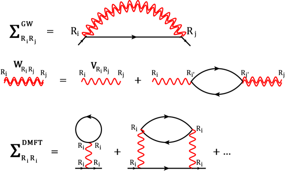
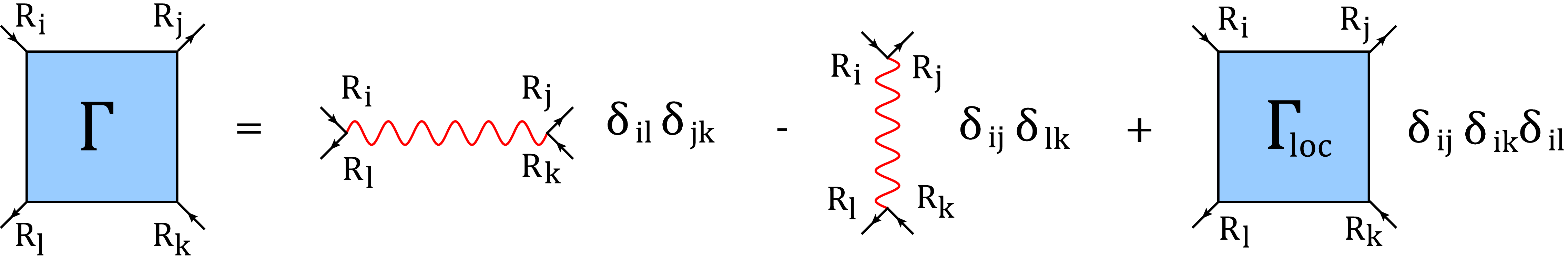
Figure 1: First line: In $GW$ the self energy $\Sigma$ is given by the interacting Green function $G$ (black straight line) times the screened interaction $W$ (red wiggled line) from coordinate/site $R_{i}$ to $R_{j}$. Second line: The screened interaction $W$ in turn is given by the bare interaction (here denoted as $V$) and the screening in the random phase approximation (RPA). This RPA screening is generated by the last term which yields a ladder in terms of $V$ and bubbles consisting of two Green functions. Third line: In DMFT the self energy is given by the local contribution of all Feynman diagrams with the local interaction $U$ always on the same site $R_{i}$. Fourth line: In AbinitioD$\Gamma$A, we take as the irreducible vertex $\Gamma$ the bare non-local Coulomb interaction $V^{q}$ and the local vertex $\Gamma_{\rm loc}$ which depends on orbitals ($l$, $m$ …) and frequencies ($\nu$, $\nu^{\prime}$, $\omega$) but not momenta ($k$,$k^{\prime}$,$q$); $\Gamma_{\rm loc}$ also includes the local Coulomb interaction $U$ (adapted from Ref. Galler2016 ).

Both methods, hybrid functionals and GW, can lead to semiconductor band gaps in far better agreement with experiment Godby1988 ; Seidel1996 ; Fuchs2007 , with the $GW$ self energy acting as a “scissors operator” Godby1988 . Beyond that, $GW$ also describes quasiparticle renormalizations, finite life times, and improves on the total energies of, e.g., defects Aryasetiawan1998 ; Freysoldt_defects_RevModPhys_2014 . While hybrid functionals are one-electron-like by construction, also the GW—at least in all common implementations (see however the recent Refs PhysRevB.94.155101 ; PhysRevB.95.035139 )—is based on a Green function $G_{0}$ that is always related to a single Slater determinant. Excluding any multi-reference character in $G_{0}$, the $G_{0}W_{0}$ approach is thus not capable to treat systems in which fluctuations are strong.

Materials in which the correlation part is particularly important are, among others, transition metal oxides and heavy fermion compounds with partially filled $d$ and $f$ shells, respectively Imada1998 . For treating electronic correlations in such materials, dynamical mean field theory (DMFT) Metzner1989 ; Georges1992a (for a review see Ref. Georges1996 ) and its merger with DFT Lichtenstein1998 ; Anisimov1997 (for reviews see Refs. Kotliar06 ; Held2007 ) has been a big leap forward. DMFT takes into account a major part of the electronic correlations: the “local” ones that are confined to a single atomic site. Fig. 1 (bottom) shows the corresponding Feynman diagrams. This way, among others, quasiparticle renormalizations including kinks Nekrasov05a ; Byczuk2007 ; Toschi2009 ; Held13 , Hubbard side bands, metal-insulator transitions, and magnetism can be described much more accurately than with one-particle methods, and finite temperature properties become accessible as well. Early successes of DFT+DMFT include the calculation of the Mott-Hubbard transition in V₂O₃ Keller2004 ; Held2001a ; Poteryaev2007 ; Hansmann2013b , magnetism in Fe and Ni Lichtenstein1998 , and the $\alpha$-$\gamma$ transition in Ce Held2001 ; McMahan2003 . More recently, it has also been applied to oxide heterostructures Okamoto2005 ; Hansmann2009 ; PhysRevLett.114.246401 , surfaces PhysRevLett.115.236802 , nanoclusters Valli2015a and oxygen vacancies PhysRevB.94.241110 .

The major remaining shortcomings of DFT+DMFT are (i) the sand in the clockwork when interfacing a density functional theory with a Feynman diagrammatic approach and (ii) that only local correlations are taken into account in DMFT. Regarding (i), let us in particular mention the double counting: It is unclear which part of the DMFT correlations are taken into account already on the DFT side, and so different double counting schemes have been proposed. Most commonly used is the fully localized limit Anisimov1991 . The double counting issue is particularly pronounced in so-called “$d+p$” DFT+DMFT calculations that in, say, oxides, include both, the transition metal $d$- as well as the oxygen $p$-orbitals and can lead to largely different results Hansmann2014 ; Dang2014 ; Haule2014 .

This conceptual problem can be overcome by substituting DFT by $GW$ in the so-called GW+DMFT approach Sun02 ; Biermann2003 , which merges two many-body Feynman diagrammatic approaches so that one can precisely identify which diagrammatic contribution is counted twice. GW+DMFT also provides for a better treatment of the exchange contribution. This is not only of advantage for correlated semiconductors such as Ga_1-xMn_xAs, and ligand-states in, e.g., transition metal oxides Tomczak12 , but also for a quantitative description of effective masses of correlated electrons Tomczak14 . We discuss the GW+DMFT approach and present results in Section 3; for a more detailed introduction we refer the reader to Refs. Held2011 ; gwdmft_proc1 ; 0953-8984-26-17-173202 ; 0953-8984-28-38-383001 . One should note, however, that the treatment of non-local correlations is very limited in GW+DMFT as only charge fluctuations and only the particle-hole channel are included in GW. Moreover they are treated only in weak coupling perturbation theory, i.e., by building the particle-hole ladder only in terms of the bare Coulomb interaction $V$, see Fig. 1 (middle).

There are essentially two routes that deal with non-local correlations while keeping the local DMFT correlations at the same time: cluster Hettler1998 ; Lichtenstein2000 ; Kotliar2001 and diagrammatic extensions Toschi07 ; Kusunose06 ; Rubtsov2008 ; Rohringer2013 ; Taranto2014 ; Ayral2015 ; Li2015 of DMFT. The former have been successfully applied to the two dimensional Hubbard model and helped establishing the presence of superconductivity in this model. However, due to numerical restrictions, realistic multi-orbital calculations are only possibly for a handful of sites, restricting the cluster extensions essentially to nearest neighbor correlations (for a review see Ref. Maier05 ).

Diagrammatic extensions of DMFT on the other hand can treat short- and long-range correlations on an equal footing, which allowed, among others, the calculation of critical exponents Rohringer2011 ; Hirschmeier2015 ; Antipov2014 ; Schaefer2016 and revealed the absence of a metal-insulator transition in the two-dimensional Hubbard model on a square lattice Schaefer2015-2 . In Section 4 we discuss the first of these diagrammatic extensions, the dynamical vertex approximation (D$\Gamma$A) Toschi07 ; Katanin2009 and its extension to ab initio calculations. For the latter, AbinitioD$\Gamma$A Toschi2011 ; Galler2016 , we take as the vertex (irreducible in the particle-hole channel) the bare non-local Coulomb interaction as well as the local Coulomb interaction and all local vertex diagrams, see Fig. 8. From this unifying framework, we naturally generate all (local and non-local) GW diagrams, all local DMFT diagrams, as well as non-local diagrams beyond. The latter include, e.g., spin fluctuations which are important in the vicinity of phase transitions, for magnons and pseudogap physics. For a pedagogical introduction see Ref. Held2014 , and Ref. Georgthesis2013 for an elaborate presentation.

2 Hedin’s GW method: The new VASP implementation

2.1 Method

Hedin’s method is in principle an exact approach to describe many-body interactions Hedin1965 ; strinati1980 ; hybertsen1986 ; Aryasetiawan1998 ; bechstedt2009 . However, in practice for computational reasons, virtually all implementations of this method are limited to the so-called $GW$ approximation. This greatly simplifies the calculations, but also makes important approximations; the considered Feynman diagrams are shown in the top panel of Fig. 1.

The new aspect of the present VASP implementation Liu2016 is that it is tuned for massively parallel computers and that it works in imaginary time and frequency as opposed to the earlier VASP implementation that worked along the real frequency axis Shishkin2006 ; ShishkinPRL2007 and necessitated very fine frequency grids. In the following, we will give a brief outline of the computational steps of the present code, highlighting why it is particularly convenient for a combination with DMFT. We follow previous publications but emphasize simplicity and conciseness by dropping for instance the Brillouin zone index as well as the PAW formalism Liu2016 . The first step in a $GW$ calculation is to determine the DFT one-electron orbitals $\psi_{i}$ and one-electron energies $\epsilon_{i}$. From the DFT orbitals the one-electron Green function follows:

$$G(\mathbf{r},\mathbf{r}^{\prime},\mathrm{i}\tau)= \phantom{-}\sum\limits^{\text{\phantom{u}occ\phantom{n}}}\limits_{i}\psi_{i}(\mathbf{r})\psi^{*}_{i}(\mathbf{r}^{\prime})\mathrm{e}^{-(\epsilon_{i}-\mu)\tau}\quad(\tau<0),$$ (1)

$$G(\mathbf{r},\mathbf{r}^{\prime},\mathrm{i}\tau)= -\sum\limits^{\text{unocc}}\limits_{a}\psi_{a}(\mathbf{r})\psi^{*}_{a}(\mathbf{r}^{\prime})\mathrm{e}^{-(\epsilon_{a}-\mu)\tau}\quad(\tau>0).$$ (2)

Generalization to finite temperature is straightforward and involves restriction of the time to $-\beta\leq\tau\leq\beta$, where $\beta$ is the inverse temperature, and introduction of Fermi occupancy factors $n_{i}=1/(\exp((\epsilon_{i}-\mu)\beta)+1)$ and $(1-n_{i})$ in the first and second equation, respectively. It is then easy to show that the function observes the anti-periodicity for Fermionic Green functions $G(\mathbf{r},\mathbf{r}^{\prime},\mathrm{i}\tau)=-G(\mathbf{r},\mathbf{r}^{\prime},\mathrm{i}(\tau-\beta))$.

As typically done in plane wave codes, all functions are expanded in a plane wave basis and fast Fourier transformed (FFT) to real space only when this is required:

$$G(\mathbf{r},\mathbf{r}^{\prime},\mathrm{i}\tau) = \sum\limits_{\mathbf{g},\mathbf{g}^{\prime}}\mathrm{e}^{\mathrm{i}\mathbf{g}\mathbf{r}}G(\mathbf{g},\mathbf{g}^{\prime},\mathrm{i}\tau)\mathrm{e}^{-\mathrm{i}\mathbf{g}^{\prime}\mathbf{r}^{\prime}}$$ (3)

$$G(\mathbf{g},\mathbf{g}^{\prime},\mathrm{i}\tau) = \frac{1}{N_{\bf r}^{2}}\sum\limits_{\mathbf{r},\mathbf{r}^{\prime}}\mathrm{e}^{-\mathrm{i}\mathbf{g}\mathbf{r}}G(\mathbf{r},\mathbf{r}^{\prime},\mathrm{i}\tau)\mathrm{e}^{\mathrm{i}\mathbf{g}^{\prime}\mathbf{r}^{\prime}}.$$ (4)

Here $N_{\bf r}$ is the total number of real-space grid points. Since the plane-wave basis can be chosen to be significantly smaller than the number of real space grid points Payne_RevModPhys_1992 , the plane wave expansion typically reduces the storage demand by a factor 6-8 for orbitals (one position index), and a factor $6^{2}-8^{2}$ for Green functions (two position indices). The first crucial approximation of the $GW$ method is that the irreducible polarizability is approximated by the independent particle polarizability (RPA). Assuming a factor 2 for spin-degenerate systems, we get

$$P(\mathbf{r},\mathbf{r}^{\prime},\mathrm{i}\tau)=2G(\mathbf{r},\mathbf{r}^{\prime},\mathrm{i}\tau)G(\mathbf{r}^{\prime},\mathbf{r},-\mathrm{i}\tau)=2G(\mathbf{r},\mathbf{r}^{\prime},\mathrm{i}\tau)G^{*}(\mathbf{r},\mathbf{r}^{\prime},-\mathrm{i}\tau),$$ (5)

that is, vertex corrections of the form $P=2GG\Gamma$ are neglected. This approximation neglects important many body effects, for instance excitonic effects ShishkinPRL2007 ; Freysoldt_defects_RevModPhys_2014 that are captured by particle-hole ladder diagrams. It has been shown that these terms become important when selfconsistent calculations are performed ShishkinPRL2007 . From the irreducible polarizability the screened interaction (see Fig. 1 middle) can be determined by:

$$W({\bf r},{\bf r}^{\prime},\mathrm{i}\omega)=V({\bf r},{\bf r}^{\prime})+V({\bf r},{\bf s})P({\bf s},{\bf s}^{\prime},\mathrm{i}\omega)W({\bf s}^{\prime},{\bf r}^{\prime},\mathrm{i}\omega)\;\Leftrightarrow\;W^{-1}=V^{-1}-P.$$ (6)

Here, $V$ is the Coulomb kernel, and integration over repeated spatial coordinates ($\bf s$ and ${\bf s}^{\prime}$) is assumed. For reasons of computational efficiency, the calculation is more conveniently done in reciprocal space, where the Coulomb kernel is diagonal Liu2016 .

The Dyson-like equation for the screened interaction needs to be solved in frequency space $\mathrm{i}\omega$. This obviously requires one to perform a Fourier transformation of the independent particle polarizability from imaginary time [compare Eq. (5)] to imaginary frequency. In previous (imaginary time) $GW$ codes Godby1995 ; Godby2000 this was a fairly cumbersome operation involving fitting, a fast Fourier transformation, and some analytic continuation at very large frequencies and times. Using a mathematical rigorous treatment, Kaltak et al. determined imaginary time and frequency grids KaltakJCTC2014 that have a number of favorable properties. (i) The grids are non-uniformly spaced. This allows to simultaneously and accurately describe intra-band transitions at very small energies (meV), as well as high energy excitations into continuum like states (up to several 100 eV). (ii) The time and frequency grids are individually optimized to allow accurate calculations of the correlation energy in second order. Convergence of the correlation energy is exponential in the number of time or frequency points, with 20 points yielding $\mu$eV convergence even for metals. (iii) The grids are dual to each other: if a Bosonic function is known at a grid of $N_{\omega}$ frequency points $\omega_{k},k=1,...,N_{\omega}$, the numerical error in the Bosonic function is minimal at a set of corresponding $N_{\tau}=N_{\omega}$ imaginary time points $\tau_{j},j=1,...,N_{\tau}$. (iv) Related to point (iii), a numerical discrete Fourier transformation exists to transform any function from imaginary time to imaginary frequency (and vice versa):

$$f(\mathrm{i}\omega_{k})=\sum\limits_{j=1}^{N_{\omega}}\gamma_{kj}\mathrm{cos}(\omega_{k}\tau_{j})(f(\mathrm{i}\tau_{j})+f(-\mathrm{i}\tau_{j}))+\mathrm{i}\,\lambda_{kj}\mathrm{sin}(\omega_{k}\tau_{j})(f(\mathrm{i}\tau_{j})-f(-\mathrm{i}\tau_{j})).$$ (7)

This is a numerical approximation to the Fourier transformation from time to frequency :

$$f(\mathrm{i}\omega) = \int_{-\infty}^{\infty}f(\mathrm{i}\tau)e^{\mathrm{i}\omega\tau}d\tau$$ (8)

$$= \int_{0}^{\infty}\Big{[}\cos(\omega\tau)(f(\mathrm{i}\tau)+f(-\mathrm{i}\tau))+\mathrm{i}\sin(\omega\tau)(f(\mathrm{i}\tau)-f(-\mathrm{i}\tau))\Big{]}d\tau.$$

The corresponding matrix of coefficients, e.g., $\gamma_{kj}\mathrm{cos}(\omega_{k}\tau_{j})$, are precalculated and stored.

The evaluation of the self energy is most conveniently done in imaginary time

$$\Sigma^{c}({\bf r},{\bf r}^{\prime},\mathrm{i}\tau)=-G({\bf r},{\bf r}^{\prime},\mathrm{i}\tau)W^{c}({\bf r},{\bf r}^{\prime},\mathrm{i}\tau),\qquad W^{c}(\mathrm{i}\omega)=W(\mathrm{i}\omega)-V\;$$ (9)

with the bare Coulomb kernel $V$ subtracted before the Fourier transformation of $W$ and the contribution $GV$ calculated analytically. As for the polarizability, also Eq. (9) neglects vertex corrections ($\Sigma=-GW\Gamma$). For non-correlated semiconductors, the vertex contributions are only of the order of 0.2 eV for states close to the Fermi-level but can reach up to 1 eV for localized $d$-orbitals Gruneis_IP_solids_2014 .

With the evaluation of $\Sigma^{c}$, a single shot $G_{0}W_{0}$ calculation is finished, so it is worthwhile to recapitulate what can be done with the yet calculated quantities. It is straightforward to express the self energy in any basis, for instance, a set of localized Wannier functions and to export it to a DMFT solver. The advantages over a conventional $GW$ implementation are numerous. (i) First, many $GW$ codes avoid calculating the full frequency dependency of the self energy, and instead evaluate the self energy only at a few points close to the DFT one-electron energies $\Sigma(\epsilon^{\rm DFT}_{i})$. In the present code, this is no longer necessary and one obtains the self energy at all imaginary time points by Eq. (9). There is a (small) price to pay, though: to obtain physically measurable quantities, the self energy needs to be continued to the real axis, for which continued fractions are used Liu2016 . However, since DMFT solvers usually work in imaginary time, the interface between VASP and DMFT is simple and requires only an interpolation from the few available imaginary frequency points $\{\mathrm{i}\omega_{i}\}$ to a denser Matsubara grid. (ii) Each of the individual compute steps scales (at worst) cubic in the number of grid points or plane waves and linear in the number of k-points, as opposed to conventional $GW$ codes, which scale quartic in the number of basis functions and quadratic in the number of k-points. The favorable scaling is straightforward to see: the calculation of the polarizability [Eq. (5)] and self energy [Eq. (9)] are clearly quadratic in the number of grid points, however, cubically scaling rank one updates of matrices and matrix multiplications are required to calculate the Green function [Eq. (1)] and the screened potential [Eq. (6)]. This favorable scaling combined with the efficient frequency grids allowed for efficient calculations of the random phase approximation (RPA) of the correlation energy for isolated defects in huge supercells containing several hundred atoms KaltakPRB2014 . (iii) The constrained RPA (cRPA) Aryasetiawan2004 is simple and straightforward to implement in the present code. One only needs to remove the polarizability $P^{t}(\mathrm{i}\tau)=2G^{t}(\mathrm{i}\tau)G^{t}(-\mathrm{i}\tau)$ of some target, say $t_{\text{2g}}$, orbitals from the total polarizability $P=P^{r}+P^{t}$ to obtain an effective screened interaction $U$:

$$U^{-1}(\mathrm{i}\omega)=V^{-1}-P^{r}(\mathrm{i}\omega)\quad\Leftrightarrow\quad U^{-1}(\mathrm{i}\omega)=W^{-1}(\mathrm{i}\omega)+P^{t}(\mathrm{i}\omega).$$ (10)

The polarizability $P^{r}(\mathrm{i}\omega)$ then captures all screening effects, except for the one inside the target space, which will be treated in the DMFT solver. The full frequency-dependent $U(\mathrm{i}\omega)$ can be calculated with very little extra cost, and after transformation from the plane wave basis to a localized target space, it can be directly imported into a DMFT continuous time quantum Monte Carlo solver.

The advantages of the imaginary time and imaginary frequency representation are more obvious if self-consistency is considered. Once the $GW$ self energy is known, the Green function can be updated by

$$G^{c}(\mathrm{i}\omega)=(\mathrm{i}w+\mu-H^{\rm HF}-\Sigma^{c}+[\Sigma_{imp}-\Sigma^{GW}_{imp}])^{-1}-(\mathrm{i}w+\mu-H^{\rm HF})^{-1},$$ (11)

where $H^{\rm HF}=-\nabla^{2}/2+V^{\rm ion}+V^{\rm H}+V^{x}$ is the Hartree-Fock Hamiltonian consisting of the kinetic energy term, the ionic $V^{\rm ion}$, Hartree $V^{\rm H}$ and exact exchange potential $V^{x}$. To obtain a converging Fourier transformation when transforming to the imaginary time, the Hartree-Fock Green function (second term) needs to be subtracted and added back in imaginary time

$$G(\mathrm{i}\tau)=G^{c}(\mathrm{i}\tau)+G^{\rm HF}(\mathrm{i}\tau).$$ (12)

This closes the cycle and allows to continue with a re-evaluation of the independent particle-hole polarizability in Eq. (5). Clearly, it is also possible to add any local self energy in Eq. (11) (terms in square brackets) and, thus, seamlessly incorporate DMFT results. Likewise, the irreducible polarization propagator can incorporate local effects beyond the independent particle-hole approximation, if the DMFT code provides the required information ($P\rightarrow P^{GW}+P_{imp}-P^{GW}_{imp}$, compare next section). This opens the route towards a concise implementation of GW+DMFT, as discussed in the next section (see Fig. 5). A closure of the self-consistency cycle is already possible in the present code, although some intricacies for metallic systems still need to be solved, including an approximate inclusion of Drude-like metallic screening, and an efficient update of the chemical potential, which is important to achieve robust convergence in the self-consistency cycle for metals.

2.2 Results

The $GW$ method has now been used for almost five decades. However, despite its undisputed improvements compared to DFT, results vary significantly between different codes. Errors are actually particularly large for transition metal compounds placing a serious question mark on any quantitative predictions. Specifically in oxides, $d$-binding energies can vary by up to 1 eV using different codes and implementations KlimesKaltak_predictiveGW_2014 . This is clearly unacceptable, if one aims to merge $GW$ with more accurate methods such as DMFT. One major problem of the $GW$ method is that the convergence with respect to the basis set size is extremely slow shih2010 ; friedrich2011 . Specifically, for the projector augmented wave method, as used in VASP, the partial waves, which are supposed to form a sufficiently complete basis in the vicinity of the atoms, need to be chosen such that basis set convergence can be attained. The slow convergence has been rigorously discussed by Klimes, Kaltak and Kresse in Ref. KlimesKaltak_predictiveGW_2014 . Although that paper also establishes a suitable benchmark for solid state systems, we are not aware that other comparable reference numbers have yet been published for solids. Then, how can one ascertain that the numbers predicted with VASP are accurate and reproduce the infinite basis set limit? Fortunately, the new VASP $GW$ code allows us to address this issue. Since it is efficient for large unit cells and large basis sets, it is possible to compare the results for molecules with atomic codes that use Gaussian type orbitals (GTOs). GTOs have been used for 50 years in quantum chemistry and have matured to a point where convergence for excited state calculations can be obtained fairly easily, although careful basis set extrapolations are as important as for plane waves.

Fig. 2 shows the difference between the basis set extrapolated GTO results and the VASP PAW results for the ionization potential of 100 closed shell molecules. The mean deviation between both codes is only 60 meV MaggioPeitao_GW100_2017 , and large outliers are practically absent. We note that the deviations between other plane wave codes and GTOs are on average twice as large, but can even reach 200 meV on average. The other important point is the large difference between theory and experiment highlighting how limited the precision of $G_{0}W_{0}$ is even for simple weakly correlated systems such as small molecules. This clearly underlines the need to go beyond the random phase approximation and single shot $G_{0}W_{0}$ calculations.

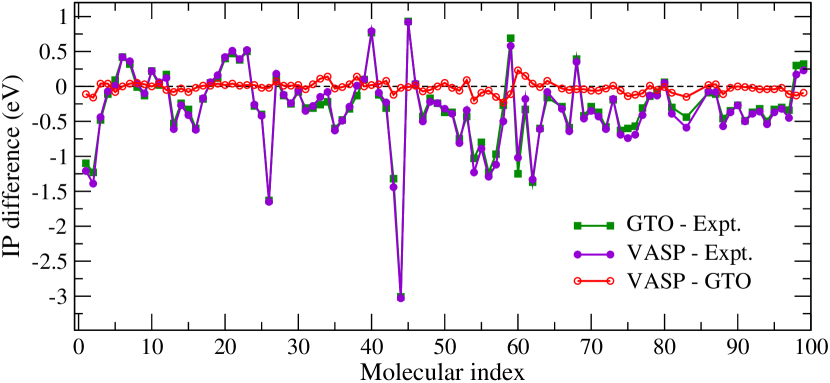
Figure 2: Difference between GTO, PW and experimental values for the ionization potential (IP) for a set of 100 molecules. The theoretical data are from $G_{0}W_{0}$ calculations using GGA orbitals (the data have been collected from Ref. MaggioPeitao_GW100_2017 ).

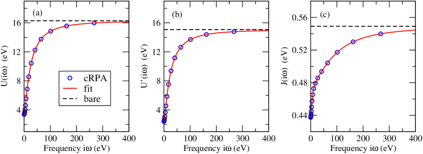
Figure 3: On-site dynamical partially screened (a) intra-orbital interactions $U(\mathrm{i}\omega)$, (b) inter-orbital $U^{\prime}(\mathrm{i}\omega)$, and (c) Hund’s coupling $J(\mathrm{i}\omega)$ of SrVO₃ as a function of the imaginary frequency (shown in blue circle). The bare counterparts are also shown as black dashed lines. The red solid lines are obtained from a Padé fit. We use 20 optimized imaginary frequency grid points and $8\times 8\times 8$ $k$ points in the calculations.

As an illustrative example for solid state calculations, we show results for SrVO₃. Fig. 3 shows our calculated on-site dynamical screened intra-orbital interaction $U(\mathrm{i}\omega)$, inter-orbital $U^{\prime}(\mathrm{i}\omega)$, and Hund’s coupling $J(\mathrm{i}\omega)$ of SrVO₃ using the cRPA and V-$t_{\text{2g}}$-like maximally localized Wannier functions. In imaginary frequency, $U$, $U^{\prime}$ and $J$ are rather smooth functions, so that it is possible to interpolate them from the optimized frequency grid to Matsubara frequencies by a Padé interpolation Vidberg1977 (see the red solid lines in Fig. 3). This makes it possible to transfer them to a dynamical impurity solver. In the static limit ($\omega=0$), $U$, $U^{\prime}$, and $J$ are calculated to be 3.38, 2.42, and 0.44 eV, respectively, agreeing perfectly with the ones directly obtained from the conventional implementation working on the real frequency axis. Moreover, they are in nice agreement with the published values Aryasetiawan06 ; PhysRevB.86.165105 . In the high-frequency limit ($\omega\rightarrow\infty$), $U$, $U^{\prime}$, and $J$ approach the unscreened (bare) counterparts (16.29, 15.07, and 0.55 eV).

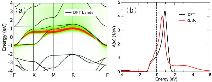
Figure 4: (color online) (a) Momentum resolved spectral function in the $G_{0}W_{0}$ approximation (color/gray) and DFT (black line). (b) Comparison of the DFT and local $G_{0}W_{0}$ spectral function $A(\omega)$.

Figure 4(a) shows the single-shot $G_{0}W_{0}$ momentum resolved spectral function. Compared to DFT, the $t_{\text{2g}}$ bandwidth is reduced by 20 % in $G_{0}W_{0}$. In the $G_{0}W_{0}$ approximation, spectral weight is transferred to satellites. This is much more clearly seen in the local, momentum-integrated, spectral function as shown in Fig 4(b). The plasmon satellite of the $t_{\text{2g}}$ quasi-particle band at $\sim$3 eV arising from the $t_{\text{2g}}$ contribution to the fully screened interaction at the plasmon frequency Tomczak12 ; PhysRevB.94.201106 is well reproduced. Further, a plasmon peak deriving from transitions outside the $t_{\text{2g}}$ subspace is seen at $\sim$15 eV Aryasetiawan06 ; Tomczak12 . We note, however, that in our calculations repeated plasmon peaks at higher frequencies are absent. This is a well known issue of the $G_{0}W_{0}$ approximation PhysRevLett.107.166401 .

3 Screened exchange and local quantum fluctuations: GW+DMFT

3.1 Method

The key advantage of the GW approach discussed above is its treatment of dynamical screening: While standard electronic structure methodologies—such as Hartree-Fock or DFT—work with the bare Coulomb interaction $V$, GW explicitly incorporates the polarizability of the electronic system. As a consequence, the repulsion between electrons becomes reduced and retarded. The resulting screened-exchange self energy yields a much improved description of, e.g., $sp$-semiconductors gaps, whereas the retardation effects account for spectral weight transfers to (plasmon) satellite features, and finite lifetimes of electronic excitations.

However, as already mentioned in the Introduction, the perturbative GW approach is insufficient for strongly correlated materials. In fact, it fails to account for their strong mass renormalizations, Hubbard satellites, and local moments physics Imada1998 . Our recent understanding of strong electron-electron correlations was indeed propelled by the advent of a non-perturbative technique: the dynamical mean field theory Georges1996 . The latter maps the lattice problem onto the self-consistent solution of an Anderson impurity model, and the lattice self energy is identified with the single-site (i.e., local) self energy of the impurity Georges1992a . This mapping becomes exact in the limit of infinite lattice coordination Metzner1989 . By construction, DMFT accounts only for correlations from on-site interactions, yet it includes—as depicted in Fig. 1—all Feynman diagrams built from the Hubbard $U$ and Hund $J$ interactions and the local impurity propagator. To set up a realistic DMFT calculation, the one-particle part of the Hamiltonian is taken from DFT (whence the name DFT+DMFT Lichtenstein1998 ; Anisimov1997 ) and the screened interaction parameters—$U$ and $J$—can be computed from techniques such as constrained DFT constrainedLDA , or, better, the constrained random phase approximation Aryasetiawan2004 ; miyake:085122 ; jmt_mno . However, as mentioned in the Introduction, it is not separable how the Hubbard $U$ already contributes to the DFT band-structure. so that there is the problem of “double-counting” correlations when adding the DMFT self energy.

From this brief summary it is apparent that GW and DMFT are very complementary techniques: GW has no restriction on the range of the interaction or the self energy and therefore excels for $sp$-systems. In DMFT the interaction and the self energy are by necessity localized on an atomic site, yet their non-perturbativeness allows for a reliable description of the Kondo and Mott physics realized in many $d$- or $f$-electron materials. At the same time, GW and DMFT share a common (diagrammatic) language. Therewith, both methods can profit from each other: As the RPA technique is integral part of the GW, it can provide the DMFT with a Hubbard $U$ computed from first principles [see the preceding section and Eq. (10)]. In return, DMFT susceptibilities and self energies can add local vertex corrections to all orders to Hedin’s equations for the polarization and self energy, see Eqs. (5) and (9), respectively. Contrary to DFT+DMFT, any double-counting in this combination of screening and correlations can be avoided, since a clear-cut separation is possible on the diagrammatic level.

This outlines the GW+DMFT method proposed in Ref. Biermann2003 . By elegantly combining the best of both worlds—screened exchange and local quantum fluctuations—GW+DMFT has the potential to vastly extend the realm of quantitative and predictive many-body electronic structure theory. Let us give specific examples: In many materials the separation between correlated $d$ or $f$-states and ligand $sp$-orbitals is often severely underestimated within DFT and DFT+DMFT PhysRevB.77.205112 ; 0953-8984-23-8-085601 ; PhysRevB.93.235138 ; Hansmann2014 . Yet, optical transitions between these states can actually be relevant for technological applications in, e.g., intelligent window coatings optic_epl , or eco-friendly rare-earth-based pigments jmt_cesf . Calculating the red colour of CeSF indeed required incorporating a GW correction into DFT+DMFT jmt_cesf . Non-local (inter-site) self energies à la GW were also shown to be crucial in oxides PhysRevB.89.235119 ; PhysRevB.93.235138 , intermetallics PhysRevB.82.085104 , and iron-pnictides and chalcogenides jmt_pnict , and in particular for explaining the non-magnetic nature of BaCo₂As₂ paris_sex . Moreover, important effects of dynamical screening were found, among others, in oxides PhysRevB.85.035115 ; Tomczak12 ; 0295-5075-99-6-67003 , pnictides Werner2012 ; paris_sex and cuprates PhysRevB.91.125142 . On the other side, local vertex corrections in susceptibilities beyond RPA where shown to be crucial in, both, Hubbard models Ayral2012 ; Ayral2013 and realistic materials, e.g., regarding the dynamical structure factor in iron-pnictides Park2011a ; Toschi2012 , and the absence of ferromagnetism in stoichiometric FeAl PhysRevB.92.205132 .

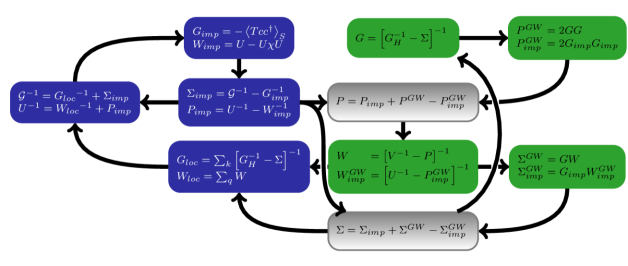
Figure 5: The GW+DMFT approach. The DMFT sub-cycle is indicated in blue, the GW procedure in green, and shared quantities in grey boxes.

After this general rationale, we will now discuss GW+DMFT in some more detail (see Refs. gwdmft_proc1 ; Held2011 ; 0953-8984-26-17-173202 ; 0953-8984-28-38-383001 for longer reviews). The workflow of the approach is depicted in Fig. 5: On the left—in blue–is the DMFT PhysRevB.52.10295 ; Si1996 ; Sun02 cycle with an additional self consistency for the two-particle interaction: It is required that the local screened interaction $W_{loc}$ equals the screened impurity interaction $W_{imp}=U+UP_{imp}W_{imp}=U-U\chi U$, where $\chi=\langle\mathcal{T}n(\tau)n(0)\rangle$ is the impurity density-density correlation function and $U$ the local interaction (containing, e.g., Hubbard and Hund terms). Owing to the dynamical nature of screening, these interactions are in particular frequency-dependent, i.e., $U\rightarrow U(\omega)$. At least for density-density type of terms, solving an Anderson impurity model with dynamical interactions is easily possible with quantum Monte Carlo techniques, both approximately PhysRevB.85.035115 and numerically exactly PhysRevB.85.035115 ; Werner10 ; PhysRevB.92.115123 . On the right—in green—are Hedin’s equations for the polarization $P^{GW}$ and the self energy $\Sigma^{GW}$ in the GW approximation. Neglecting vertex-corrections here boils it down to the RPA for $P^{GW}$, Eq. (5), and the first order $GW$ expression for $\Sigma$, Eq. (9).

DMFT and GW intersect at two junctures—marked in grey—once on the two-particle level in the polarization, and once on the one-particle/spectral level in the self energy. Both times, non-perturbative, yet local contributions from DMFT, $P_{imp}$ and $\Sigma_{imp}$, are added to the GW contributions, $P^{GW}$ and $\Sigma^{GW}$. Since the latter already contain some of the local diagrams of the former, these terms have to be subtracted. Indeed, at each iteration, we need to remove all contributions from the polarization and the self energy that arise when computing the impurity analogues of $P$ and $\Sigma$ on the GW level. In case of the polarization, this is achieved by subtracting a local RPA polarization $P^{GW}_{imp}=2G_{imp}G_{imp}$ obtained from a convolution of two impurity Green functions Nomura12 : $P=P_{imp}+P^{GW}-P_{imp}^{GW}$. For the self energy, we need to subtract a term $\Sigma_{imp}^{GW}$ that is computed as the first order contribution in an interaction $W^{GW}_{imp}$ that derives from screening the impurity interaction—the Hubbard $U$—with the above polarization $P^{GW}_{imp}$, i.e., $W^{GW}_{imp}=\left[U^{-1}-P_{imp}^{GW}\right]^{-1}$. Due to these junctures, there is an outer self-consistency that allows for a feedback of local and non-local many-body effects onto the GW and DMFT cycles, respectively. Typically such a calculation is initialized with a Green function $G=\left[G_{H}^{-1}-\Sigma\right]^{-1}$, where $G_{H}$ denotes the Hartree Green function, and a guess for the self energy $\Sigma$ (here including the Fock term). In the first iteration, $\Sigma$ is usually replaced by the DFT exchange-correlation potential $V^{xc}$, i.e., $G=G^{DFT}$ (called $G_{0}$ in the Introduction section).

3.2 Results

Combining two methods that have evolved and matured independently over decades into large software packages is an intricate endeavor. Therefore, the full scheme, as shown in Fig. 5, has been realized first for one-band calculations Sun02 ; Ayral2012 ; Ayral2013 ; Hansmann2013 . For realistic multi-band systems, the first implementation—Tomczak et al. Tomczak12 —resorts to simplifications, namely (1) omitting global self-consistency, i.e., performing only one-shot GW calculations starting with $G=G^{DFT}$, (2) fixing the double-counting polarization $P^{GW}_{imp}$ to the (dynamical!) cRPA result and approximating $P_{imp}\approx P^{GW}_{imp}$, (3) approximating the double-counting self energy by the local projection of the GW self energy: $\Sigma^{GW}_{imp}\approx\sum_{k}\Sigma^{GW}$, and (4) solving the DMFT impurity with dynamical $U(\omega)$ within the approximative Bose factor Ansatz PhysRevB.85.035115 . In other early works, additional approximations were made: Taranto et al. used a static Hubbard $U$ and circumvented computing a fully frequency-dependent $\Sigma^{GW}$Taranto2013 (see also below), and Sakuma et al. combined DMFT and GW self energies from independent calculations PhysRevB.88.235110 .

Applied to the prototypical correlated metal SrVO₃, GW+DMFT revealed important new insights Tomczak12 ; Tomczak14 : The additional ingredients—the momentum-dependent self energy $\Sigma(\mathbf{k},\omega)$ and retardation effects in the Hubbard interaction $U(\omega)$—are found to compete. The dynamics in the interaction describes, among others, spectral weight transfers to plasmon satellites (at $\sim 15$eV for SrVO₃ Aryasetiawan06 ). These high energy excitations account for an additional (i.e., beyond Hubbard-model physics) reduction of the low-energy quasi-particle weight and, correspondingly, to a narrowing of the band-width PhysRevB.85.035115 ; 0295-5075-99-6-67003 (by a factor $Z_{B}\sim 0.7$ in SrVO₃casula_effmodel ). Therefore, DMFT calculations that use only static interactions, have to employ a larger Hubbard $U=4-5.5$eV Pavarini04 ; Nekrasov05a ; PhysRevB.77.205112 ; 0953-8984-23-8-085601 than the static limit $U(\omega=0)\approx 3.5$eVAryasetiawan06 ; miyake:085122 ; Tomczak12 of the cRPA to account for the same mass enhancement; such a larger interaction is actually obtained in constrained LDA Sekiyama2004 . The non-local exchange self energy on the other hand widens the low-energy dispersion jmt_pnict ; Tomczak12 ; Miyake13 ; 0295-5075-108-5-57003 . Correspondingly, effective masses of quasi-particles are reduced. With respect to the LDA reference, effective masses are given by the ratio of the LDA and GW+DMFT group velocities:

$$\frac{m^{*\phantom{DA}}}{m^{LDA}}=\frac{d\epsilon_{\bf k}^{LDA}/dk}{dE_{\bf k}/dk},\qquad\frac{dE_{\bf k}}{dk}=\left.\frac{d\epsilon_{\bf k}^{LDA}/dk+\partial_{k}{\rm Re}\Sigma({\bf k},\omega)}{1-\partial_{\omega}{\rm Re}\Sigma({\bf k},\omega)}\right|_{{\bf k}={\bf k_{F}},\omega=0}\;.$$ (13)

Here, the denominator is related to the quasi-particle weight $Z_{\bf k}=[1-\partial_{\omega}{\rm Re}\Sigma({\bf k},\omega)]^{-1}_{\omega=0}$. In DMFT, where the self energy is local, $m^{*}/m^{LDA}=1/Z$ holds. In GW+DMFT, the extra term involving the momentum derivative of the self energy substantially counteracts the mass enhancement generated by the dynamical correlations jmt_pnict ; Tomczak14 . Altogether this yields a similar effective mass as in the previous DFT+DMFT calculations (that use $U>U(\omega=0)$), but the low-energy spectral weight is different, and can be measured by transport or optics.

In Fig. 6 we compare Matsubara self energies for the $t_{\text{2g}}$ orbitals of SrVO₃ obtained with our new implementation that combines the GW-code of VASP detailed in Section 1 with the w2dynamics DMFT code Parragh12 ; Wallerberger16 . We employ the same approximations (1)-(3) as in Ref. Tomczak12 . However, instead of (4) the approximative Bose-factor Ansatz PhysRevB.85.035115 , we use a numerical exact continuous-time quantum Monte Carlo algorithm for retarded density-density interactions Werner10 . Our reference is a standard DFT+DMFT calculation that uses a static Hubbard $U(\omega=0)$ and Hund’s $J$ as provided by the cRPA (see Fig. 3). From the low-energy slope of ${\rm Im}\Sigma(i\omega_{n})$ we extract a quasi-particle weight $Z=0.6$. Turning on the retardation in the interaction, i.e. solving DFT+DMFT with the dynamical cRPA $U(\omega)$ adds substantial renormalizations of plasmonic origin; $Z$ decreases to 0.3. Moreover, since the dynamical interaction recovers at high frequencies the unscreened Coulomb interaction, ${\rm Re}U(\omega\rightarrow\infty)\approx 16$eV, also the self energy $\Sigma$ lives on a much larger energy scale PhysRevB.85.035115 than in the standard, static DFT+DMFT case. Adding the non-local GW self energy decreases effective masses, i.e. the ratio of $U$ over bandwidth diminishes and so does the strength of correlations: In our GW+DMFT the local quasi-particle weight is $Z=0.63$, which is even slightly larger than within static DFT+DMFT. We find qualitative agreement with previous GW+DMFT results from Ref. Tomczak14 .

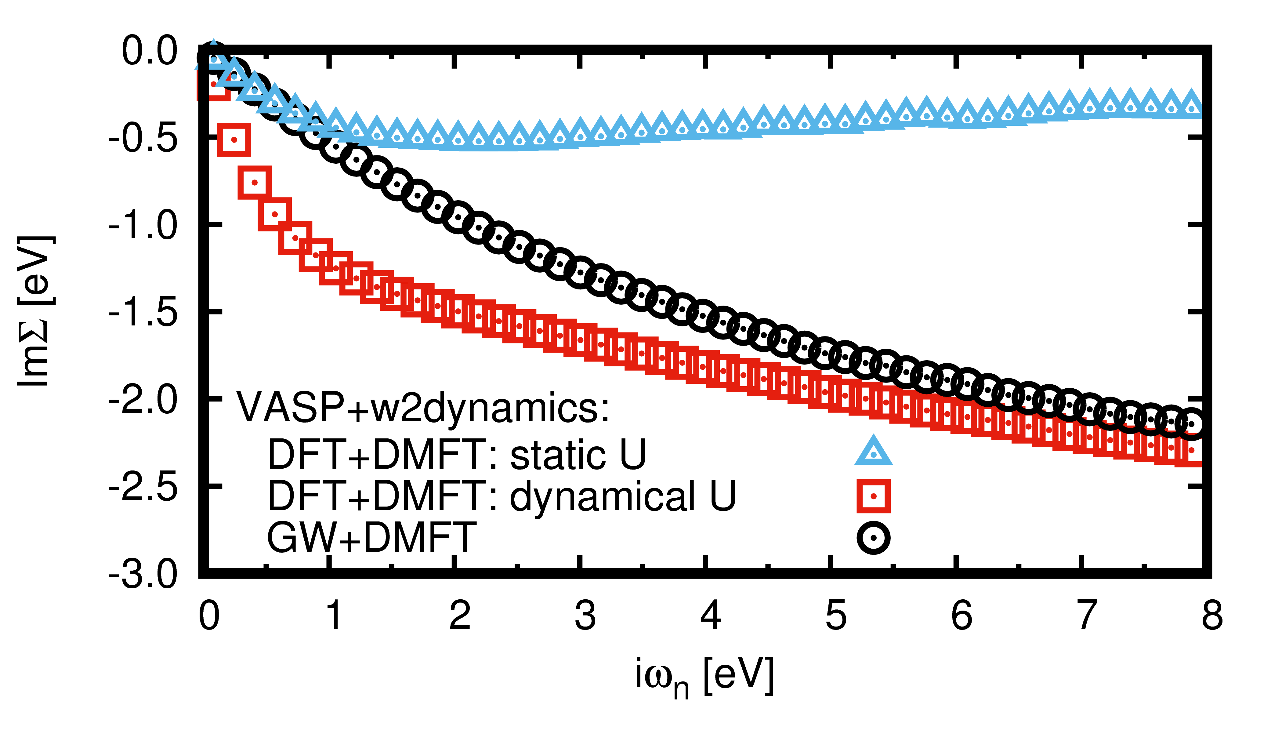
Figure 6: Local Matsubara self energies ($T=300$K) for the $t_{\text{2g}}$ orbitals of SrVO₃ using (i) DFT+DMFT with static $U=U(\omega=0)$, (ii) DFT+DMFT with the dynamical interaction $U(\omega)$ from cRPA, and (iii) GW+DMFT. Data obtained using the new GW implementation of VASP in combination with w2dynamics.

GW+DMFT spectra for the $t_{\text{2g}}$-orbitals of SrVO₃ from Ref. Tomczak12 are shown in Fig. 7 in comparison with angle-resolved photoemission spectroscopy (ARPES) results. The calculation agrees well with the experimental data. Differences to previous DFT+DMFT calculations (see, e.g., Refs. Pavarini04 ; Nekrasov05a ; PhysRevB.77.205112 ; 0953-8984-23-8-085601 ) are however most pronounced for unoccupied states Tomczak14 , that are inaccessible to ARPES experiments. The effects are in line with the above discussion: (i) W.r.t. DFT+DMFT the low-energy bandwidth is enhanced by non-local self energy contributions (e.g., the unoccupied $d_{xy}$, $d_{xz}$-bands at the X point move up from 0.6eVNekrasov05a to $\sim 1$eV). (ii) Using an ab initio screened interaction $U(\omega)$ (instead of a larger static $U$ adjusted so as to reproduce the experimental mass enhancement), the upper Hubbard band is placed at much lower energy (e.g., 1.2(1.9)eV instead of 2.2(2.85)eV Nekrasov05a at the $\Gamma$(X) point for the $d_{xy}$, $d_{xz}$-components). Indeed, the upper Hubbard band merges with the quasi-particle peak in momentum-integrated spectra. This reduced importance of Hubbard physics has recently been confirmed by partially self-consistent GW+DMFT calculations PhysRevB.94.201106 , and is compatible with recent inverse ARPES experiment. Besides the shown low-energy dispersion, also the position of ligand states, in particular the O-$2p$ and Sr-$4d$ improve substantially in GW+DMFT. Since the discussed GW+DMFT results are not globally self-consistent, the ligand states are at the same position as in $G_{0}W_{0}$ calculations Tomczak12 ; Taranto2013 ; Tomczak14 ; Kazuma16 .

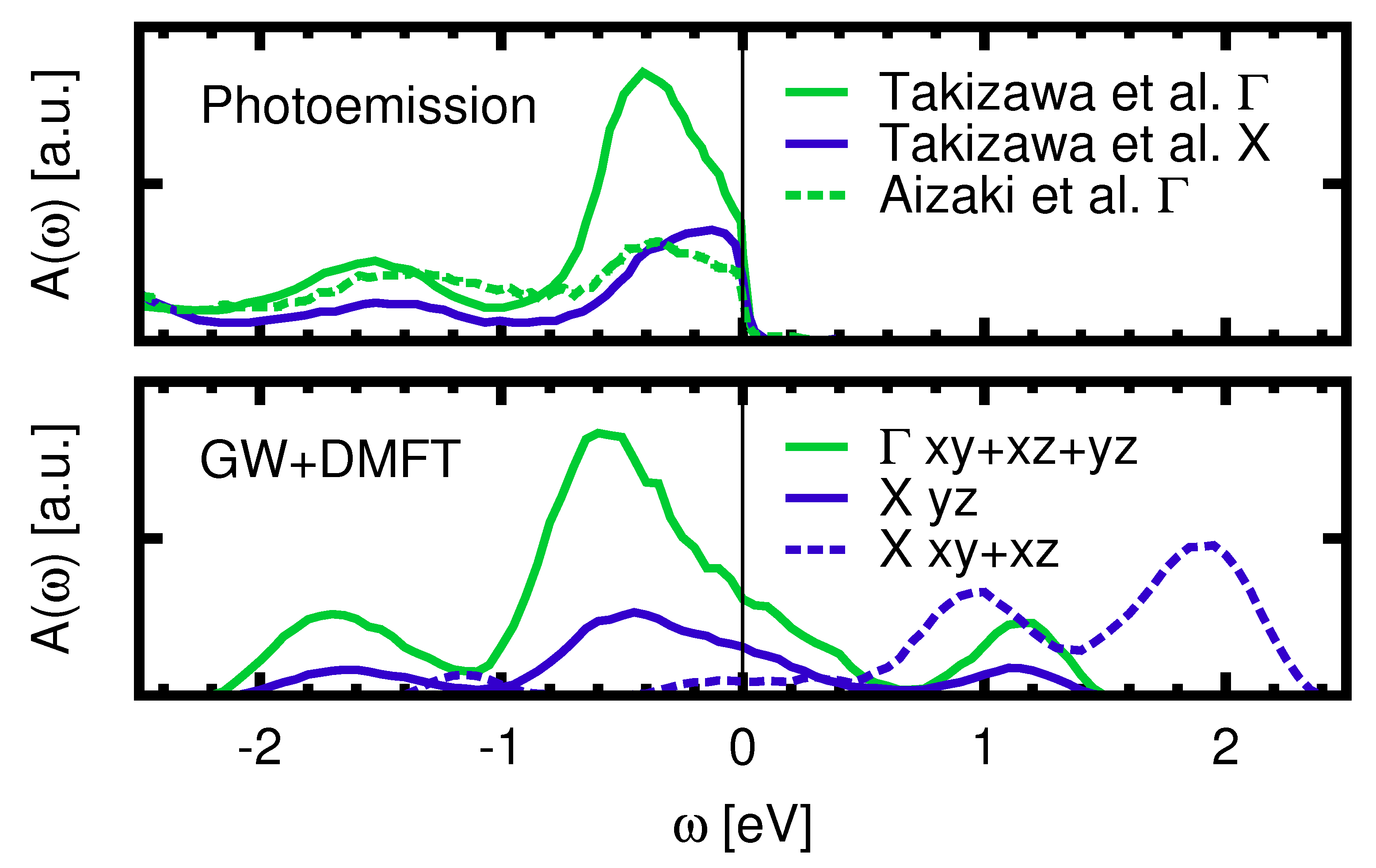
Figure 7: Comparison of GW+DMFT spectra from Ref. Tomczak12 (bottom) with angle resolved experimental photoemission spectra (top) from Refs. Aizaki12 ; PhysRevB.80.235104 for the $\Gamma$ and $X$-point.

In the setup used for these results (one-shot $G_{0}W_{0}$), the only modification of the DMFT code comes from adding the frequency- and momentum dependent GW self energy contributions into the DMFT one-particle self-consistency. Yet, since the GW self energy is a large and unhandy object, it stands to reason to approximate it to alleviate memory consumption. Also, as mentioned in the preceding section, some GW codes cannot provide the self energy on a continuous frequency mesh. A strategy to simplify the influence of the GW self energy was pioneered by Taranto et al. in Ref. Taranto2013 : By evaluating the self energy at the Kohn-Sham energies and hermitianizing it along the lines of Ref. Faleev2004 , it is possible (using an approximate double-counting correction) to cast $\Sigma^{GW}$ into Hamiltonian form. This idea was further developed into the more rigorous quasi-particle self-consistent (QS)GW+DMFT approach proposed by Tomczak in Ref. jmt_sces14 —previously alluded to in Ref. jmt_pnict —in which the double-counting correction can be performed exactly, and furthermore, a global self-consistency is performed on the QSGWFaleev2004 level. Flavors of QSGW+DMFT have subsequently been applied to cuprates and nickel oxide Choi2016 , nickel and iron PhysRevB.95.041112 , as well as insightful model systems 0953-8984-27-31-315603 ; 2016arXiv161107090L . Recently, Boehnke et al.PhysRevB.94.201106 have pioneered a setup in which GW+DMFT self-consistency is performed beyond the quasi-particle approximation, yet only within a low-energy subspace, in this case the $t_{\text{2g}}$-orbitals of SrVO₃. As anticipated in earlier model calculations for the extended Hubbard model Ayral2012 ; Ayral2013 , the self-consistent local interactions are smaller in this setup than the initial cRPA values: compared to previous non-self-consistent works Tomczak12 ; Tomczak14 the strength of correlations is reduced and mass renormalizations in SrVO₃ become more plasmonic in origin PhysRevB.94.201106 .

This concludes the description of the current state-of-the-art in GW+DMFT calculations. While there is a panoply of materials to which the described methodology can be applied with great benefit, let us point out two challenges for future developments: (i) Besides influencing the low-energy dispersion, the GW self energy also effects higher lying states, e.g., the O-$2p$ and the Sr-$4d$ orbitals in SrVO₃. Indeed, the O-$2p$ orbitals are off by $1.5-2$eV within DFT, and are pushed towards their experimental position by the GW self energy Tomczak12 ; Tomczak14 ; Kazuma16 . This will reduce their contribution to screening, causing an increase in the Hubbard $U$ for the $t_{\text{2g}}$-orbitals, as indeed found when performing cRPA on top of QSGW. This effect of ligand states will counteract the reduction of correlations seen in calculations in which self-consistency is limited to the $t_{\text{2g}}$-orbitals PhysRevB.94.201106 . Hence, a GW+DMFT implementation that includes ligand states in the self-consistency is eagerly awaited. (ii) Contrary to one-shot $G_{0}W_{0}$, self-consistent GW+DMFT is a conserving theory on the one-particle level: the GW+DMFT self energy is derivable from an approximation to a free-energy functional Almbladh1999 ; Biermann2003 . Yet, on the two-particle level the situation is inverted: RPA and also QSGW+DMFT jmt_sces14 yield a conserving density-density response function/polarization. In fully self-consistent GW+DMFT which uses dressed Green functions, on the other hand, gauge invariance for the polarization is not given and its violation can lead to a qualitatively wrong description of, e.g., collective (plasmon) modes Hafermann2014a . Achieving gauge-invariance respecting one- and two-particle quantities within a GW+DMFT scheme remains a challenge for future works.

4 Correlations on all time- and length-scales: Ab initio D$\Gamma$A

4.1 Method

The essential approximation of DMFT is that the self energy $\Sigma$, which is nothing but the one-particle fully irreducible vertex, is local—given by all local skeleton diagrams Georges1996 . We can put this concept on the next level, assuming the locality of the two-particle fully irreducible vertex $\Lambda$. This is the dynamical vertex approximation (D$\Gamma$A) Toschi07 ; Katanin2009 . From the local, fully irreducible vertex $\Lambda$, extracted by inverting the local parquet equation of DMFTRohringer2012 , one can construct—through the self-consistent solution of the parquet equation of the lattice system—the non-local full vertex $F$, and from that, the non-local D$\Gamma$A self energy as well as all physical susceptibilities. This full-fledged parquet D$\Gamma$A approach has been employed in Refs. Valli2015 ; Li2016 . In most calculations however, a restriction to the particle-hole (and transversal particle-hole channel) has been employed. In this so-called ladder D$\Gamma$A Toschi07 ; Katanin2009 , the local vertices irreducible in the two particle-hole channels $\Gamma_{ph}$ are the starting point and the full vertex $F$ is constructed through the Bethe-Salpeter ladder. This neglects the particle-particle channel which is important, e.g., for superconductivity and weak localization corrections to the conductivity. In both variants the local and non-local self energy is obtained through the Schwinger-Dyson equation of motion, and includes non-local correlation effects such as spin fluctuations and pseudogap physics.

A variety of closely related approaches have been subsequently proposed Rubtsov2008 ; Rohringer2013 ; Taranto2014 ; Ayral2015 ; Li2015 . They all have in common that they include all the local DMFT correlations, and construct additional non-local correlations from the two-particle vertex via Feynman diagrams. The differences are in the details: (i) which two-particle vertex is taken, (ii) whether the real or a dual Green function (subtracting the local Green function) is taken as connection line, (iii) which Feynman diagrams are considered. These diagrammatic extensions of DMFT have been highly successful for studying model systems such as the one-band Hubbard model and we discuss selected results in Section 4.2.

For realistic materials calculations, one might envisage using D$\Gamma$A instead of DMFT in a DFT+D$\Gamma$A scheme. However, it is more appealing to use the Bethe-Salpeter equation also as a means for calculating the non-local exchange and correlation. This is possible by taking, as the irreducible vertex in the particle-hole channel, the non-local Coulomb interaction $V^{q}$ in addition to the local vertex, see Fig. 8 (b). Besides non-local interactions, such a treatment also allows us to include less strongly correlated orbitals—without the need to calculate the local vertex for them. In the following we discuss this AbinitioD$\Gamma$A, while results for SrVO₃ are presented in Section 4.3

Figure 8: Flow diagram of the AbinitioD$\Gamma$A algorithm (from Ref. Galler2016 ).

The flow diagram of the AbinitioD$\Gamma$A algorithm is given in Fig. 8, for a complete presentation and technical details see Ref. Galler2016 :

Fig. 8 (a): The first step is to calculate the local generalized susceptibility $\chi_{\rm loc}$ via the numerical solution of an Anderson impurity model, and use the local variant of the Bethe-Salpeter equation as well as the bare (bubble) susceptibility $\chi_{\rm 0,loc}$ to extract the local irreducible vertex in the particle-hole channel $\Gamma_{\rm loc}$ (as indicated). This vertex and the local susceptibility depends on three frequencies $\nu$, $\nu^{\prime}$ and $\omega$, and four orbitals $m$, $l$, $m^{\prime}$, $l^{\prime}$.

Fig. 8 (b): We supplement this local irreducible vertex $\Gamma_{\rm loc}$ with the non-local Coulomb interaction $V^{q}$ at momentum $q$. Together these terms form the AbinitioD$\Gamma$A approximation for the irreducible vertex $\Gamma^{q}$ in the particle-hole channel.

Fig. 8 (c): With this $\Gamma^{q}$ we solve the Bethe-Salpeter equation on the lattice to get the full vertex $F^{q}$.

Fig. 8 (d): This $F^{q}$ allows us in turn to calculate the AbinitioD$\Gamma$A self energy via the Schwinger-Dyson equation of motion (the second line represents the Hartree and Fock contribution to the self energy).

Self consistency: With a new self energy and local Green function we can, in principle, go back to Fig. 8 (a) and recalculate the local susceptibility and vertex, closing the self-consistency loop.

Before turning to our presentation of selected D$\Gamma$A results, let us briefly discuss what kind of physics the AbinitioD$\Gamma$A can describe. First of all, we notice that the first, $V^{q}$ term of Fig. 8 (b) yields the RPA screening when inserted into the Bethe-Salpeter equation in the particle hole of Fig. 8 (c). Via Fig. 8 (d) this yields the $GW$ self energy. That is, all $GW$ diagrams are included in AbinitioD$\Gamma$A. But on top of GW, there is also the crossing symmetrically related ladder in the transversal particle-hole channel. Second, if we only consider the local Green functions in the Bethe-Salpeter equation Fig. 8 (c), we recover the local $F$ or susceptibility $\chi$ of Fig. 8 (a) as well as, via the equation of motion, i.e., the DMFT self energy. In other words, all DMFT diagrammatic contributions are also included. Beyond both, we have more diagrams and physics included, e.g., spin fluctuations. These can be described in weak coupling perturbation theory as the particle-hole and transversal particle-hole ladder with the local bare interaction $U$ as a building block. These diagrams are generated in Fig. 8 (c) when taking the bare $U$ term which is part of $\Gamma_{\rm loc}$ in Fig. 8 (b). More precisely it is the $U$ contribution to the vertex which is analogous to the second, $V^{k-k^{\prime}}$ term on the right hand side of Fig. 8 (c) which generates the spin fluctuations. Let us emphasize that in D$\Gamma$A such spin fluctuations are not restricted to weak coupling, the same kind of diagrams are also generated with the full $\Gamma_{\rm loc}$.

4.2 Results I: One-band Hubbard model

In the last decade the D$\Gamma$A has been intensively applied to study several physical aspects of the single-orbital Hubbard model. On the one hand, this was important to demonstrate the performance of D$\Gamma$A-based algorithms to describe intermediate-to-strong-coupling parameter regions, hardly accessible to other techniques, in view of subsequent applications to realistic systems. On the other hand, the D$\Gamma$A, since its first applications to single-orbital models, has allowed significant progress in the fundamental understanding of important topics in many-body physics. We just mention here, among others, in $d=2$ the transformation of the Mott metal-insulator transition into a crossover down to $U=0$ and the spin-fluctuation-driven pseudogap Katanin2009 ; Schaefer2015-2 ; Schaefer2015-3 ; Rohringer2016a , and, in $d=3$, the critical exponents of the Hubbard model and the breakdown of the paramagnetic Fermi-liquid at low temperatures ($T$) because of spin fluctuations Rohringer2011 ; Rohringer2016a . Notably, several of these D$\Gamma$A findings have been supported Otsuki2014 ; Hirschmeier2015 by complementary results of other powerful diagrammatic-extensions of DMFT, such as the dual-fermion Rubtsov2008 and dual-boson approaches Rubtsov12 , as well as other novel many-body techniques (e.g., the fluctuation diagnostics Gunnarsson2015 ).

Figure 9: Magnetic phase-diagram of the three-dimensional Hubbard model with nearest neighbor hopping $t$ as a function of decreasing density $n$ (hole-doping), for an intermediate value of the interaction $U=9.80t$. The left and right box give the critical and quantum critical exponent $\nu$ at finite and zero $T$, respectively. The inset shows the deviation from commensurate AF order in D$\Gamma$A (adapted from Ref. Schaefer2016 ).

In this section, we will review some of the most recent D$\Gamma$A applications to the single-orbital Hubbard model in $d=3$, and discuss their possible implications for the development of high-performing multiorbital algorithms. The first D$\Gamma$A application we consider is the investigation Schaefer2016 of the quantum critical properties of the magnetic transition in the three dimensional Hubbard model, as a function of (hole-)doping. As it was also found in DMFT Jarrell1997 , the relatively high antiferromagnetic (AF) ordering temperature ($T_{N}$) of the half-filled system is progressively reduced by increasing doping, until at about $20\%$-doping a quantum critical point (QCP) is found (see Fig. 9). The reduction of $T_{N}$ is associated also to a gradual transformation of the magnetic order from commensurate AF at ($\bf\pi,\pi,\pi$) to an incommensurate spin-density wave (SDW) at $(\bf\pi,\pi,Q_{z}<\pi)$, see inset of Fig. 9. While the DMFT-description of the related (quantum) critical properties is restricted to mean-field correlations in space, the D$\Gamma$A-treatment of both space and temporal correlations on an equal footing yields an improved understanding of the magnetic QCPs in $d=3$. In particular, beyond a sizable reduction of $T_{N}$ w.r.t. DMFT throughout the phase-diagram, the finite-$T$ critical exponents $\gamma$, $\nu$ found in D$\Gamma$A for the magnetic susceptibility and correlation length, respectively, are consistent with the $3d$-Heisenberg universality class (i.e., $\gamma\simeq 1.4,\nu\simeq 0.7$), independently on whether the antiferromagnetism is commensurate or incommensurate. While this already corrects the mere mean-field values of critical exponents found in DMFT ($\gamma=1,\nu=0.5$), the nature of the criticality changes further at the QCP. Here around $n\sim 0.8$, the exponents take unexpectedly the values $\gamma\simeq 0.7\div 0.8$, $\nu=1$, strongly violating the typical scaling relation $\gamma=2\nu$. These values are also incompatible with the standard Hertz–Millis-Moriya theory Hertz1976 ; Millis1993 for perturbative QCPs. By means of a complementary semi-analytical analysis Schaefer2016c , the unusual values of the critical exponents have been ascribed to the presence of lines of Kohn’s points in the underlying Fermi surface, whose effect is no longer damped by finite-temperature fluctuations at the QCP. The D$\Gamma$A results have, thus, identified an additional, important factor controlling the quantum critical properties of correlated systems, hitherto mostly neglected.

The effects of non-local fluctuations are, obviously, not confined to the (quantum) critical properties, as they also affect the spectral properties, in particular at the Fermi-energy. However, while the electronic self energy is significantly corrected w.r.t. the DMFT results, especially at low-$T$ Rohringer2011 ; Rohringer2016a , a closer inspectionSchaefer2015 reveals that, in $d=3$, the intrinsic frequency/momentum structure of the electronic self energy in D$\Gamma$A displays specific, important patterns. These, in turn, can be used for devising important simplifications of realistic many-body algorithms for bulk systems, such as GW, GW+DMFT, or the AbinitioD$\Gamma$A.

Figure 10: Real part of the self energy $\Sigma({\bf k},\omega)$ of the Hubbard model in $d=3$ ($U=1.6$, $T=0.043$ and $n=0.9$; energies in units of the half-bandwidth), analytically continued to the real-frequency axis, computed with D$\Gamma$A (solid lines) and $GW$ (dashed lines), respectively. The curves correspond to different k-points crossing the Fermi-surface selected on two different paths in the $(k_{x},k_{y})$-planes with constant $k_{z}=0,{\pi}$ (left/right panel), as shown in the corresponding insets (adapted from Ref. Schaefer2015 ).

Specifically, an inspection of the D$\Gamma$A self energy, continued to real frequencies (see Fig. 10) shows that the self energy of the $3d$ Hubbard model, even in the most correlated low-doping regime ($n=0.9$), displays a clear separation in the time/frequency and space/momentum domains:

$$\Sigma(\bf k,\omega)=\Sigma^{\rm loc}(\omega)+\Sigma^{\rm non-loc}(\bf k).$$ (14)

The hallmark of such separation, which extends to a relatively broad frequency interval around the Fermi level, is immediately visible in Fig. 10: in form of the parallel frequency behavior of Re$\Sigma(\bf{k},\omega)$ for different ${\bf k}$, which reflects a momentum-independent quasi-particle renormalization factor $Z_{\bf k}\sim Z$. The D$\Gamma$A demonstrates, in fact, that the momentum dependence of $\Sigma(\bf k,\omega)$ is essentially confined to the static sector, which explains the shift among the different parallel self energies. Not surprisingly, the same qualitative behavior, though—quantitatively—less correlated (i.e., with a larger $Z$) is found in the corresponding $GW$ results, shown for comparison in Fig. 10. It is however noteworthy that the static momentum-dependence is much larger in D$\Gamma$A than in GW. This advocates the presence of true non-local correlation effects as opposed to exchange effects that cause a large (static) $\mathbf{k}$-dependence in multi-band GW calculations Miyake13 ; Tomczak14 . In fact, lacking spin-fluctuations (both local and non-local), GW—where space-time separation was first evidencedjmt_pnict ; Tomczak14 —verifies Eq. (14) up to larger frequencies than D$\Gamma$A.

The validity of Eq. (14) for strongly correlated systems in $d\!=\!3$ is inspiring for promising algorithmic improvements, potentially applicable to several many-body techniques (e.g., GW, GW+DMFT, AbinitioD$\Gamma$A). In all these cases, the assumption of a full time-space separability of $\Sigma(\bf{k},\omega)$ would allow to avoid numerically expensive transfer-momenta/frequency convolutions in the intermediate steps of many-body/diagrammatic calculations, reducing considerably the numerical effort. Further details about such simplifications, and an explicit proposal of a “space-time separated GW” scheme are reported in Ref. Schaefer2015 . We should also notice, at the end of this section, that complementary simplifications of the momentum structure, were suggested by the recent findings of Ref. Pudleiner2016 : In $d=2$ the momentum dependence of $\Sigma(\bf{k},\omega)$ can often be approximated by a dependence on the non-interacting dispersion, i.e., $\Sigma(\bf{k},\omega)\rightarrow\Sigma(\epsilon_{\bf k},\omega)$.

4.3 Results II: SrVO₃

Being a diagrammatic extension of DMFT, the algorithmic implementation of D$\Gamma$A is not affected by cluster-size limitations of cluster extensions of DMFT, making possible a systematic generalization of the D$\Gamma$A approach to treat realistic multiorbital systems. While the technical aspects of the AbinitioD$\Gamma$A Toschi2011 ; Galler2016 have been addressed in the previous Section, here we will discuss the physics emerging from the first applications of the AbinitioD$\Gamma$A to realistic material calculations. Specifically, we will focus on the very recent AbinitioD$\Gamma$A study of Galler et al.Galler2016 performed for the correlated-metal testbed material SrVO₃. In this compound the $3d\!-\!t_{2g}$ bands of V are rather well separated from the other bands, which allows for a relatively accurate modelization already in terms of a three-orbital $t_{\text{2g}}$-only manifold. In fact, this modelization has been exploited in the past for a huge number of many-body calculation, from LDA+DMFT to GW+DMFT (see Section 3), and represents, thus, a sort of drosophila among correlated systems.

Figure 11: Momentum-dependence in the $k_{z}$$=$$0$-plane of (a) the real and (b) imaginary part of the electronic self energy at the lowest Matsubara frequency ($i\nu_{0}$), computed in AbinitioD$\Gamma$A for the V-$t_{\text{2g}}$ orbital $3d_{xy}$ of SrVO₃. The corresponding quasi-particle parameters (weight $Z_{\bf k}$) and scattering rate $\gamma_{\bf k}$, are reported in panels (c) and (d), respectively (reproduced from Ref. Galler2016 ).

The application of the AbinitioD$\Gamma$A to SrVO₃ has allowed one of the first non-perturbative analyses of the momentum-dependence of the self energy, and of the spectral function in this compound. The AbinitioD$\Gamma$A calculation foots on a DMFT solution of a realistic three-band Hubbard model for the t_2g-orbitals of vanadium. The latter uses a static Hubbard $U=5.0$eV and Hund’s $J=0.75$eV in the rotationally-invariant Kanamori parametrization. The computation of two-particle quantities resorts to a recent worm algorithm Gunacker15 . A sample of the AbinitioD$\Gamma$A results, for the $d_{xy}$-orbital, is shown in Fig. 11, where Re$\Sigma({\bf k},i\nu)$ and Im$\Sigma({\bf k},i\nu)$ at the lowest Matsubara-frequency ($i\nu=i\nu_{0}=\pi T$) are reported, as well as the related quasiparticle parameters ($Z_{\bf k}$) and ($\gamma_{\bf k}$) extracted from a low-frequency expansion of Im$\Sigma({\bf k},i\nu_{n})$. These AbinitioD$\Gamma$A results show that that a sizable momentum dependence does appear in the electronic self energy of SrVO₃ even if—as in this case—non-local interactions are neglected. These effects thus correct the purely local DMFT results. Interestingly, this k-dependence is mostly confined to Re$\Sigma({\bf k},i\nu_{0})$ (Fig. 11a), where one observes a momentum differentiation larger than $0.2$eV, which, however, does not directly mirror the shape of the underlying Fermi-surface. At the same time, the overall k-dependence of Im $\Sigma({\bf k},i\nu_{0})$, and the related quasi-particle coefficient $Z_{\bf k}$, $\gamma_{\bf k}$ (Fig. 11b-d) is definitely much weaker (e.g., $Z_{\bf k}$ varies less than $2\%$ over the whole Brillouin zone, with an average value slightly increased w.r.t. DMFT). We note that this behavior matches rather well the conclusions of the space-time separation emerging from previous single band D$\Gamma$A calculations Schaefer2015 discussed above. Moreover, going beyond the single-orbital framework, it is also worth emphasizing that a correlation between the momentum and orbital-dependence is found: the strength of the k-dependence, as computed in Ref. Galler2016 , displays the same trends for the orbital dependence of $\Sigma$. The latter was found, indeed, to be much more pronounced for Re$\Sigma({\bf k},i\nu_{0})$, than for the other quantities shown in Fig. 11.

5 Conclusions

One of the main challenges in computational materials science is to predict the properties of materials for which the standard DFT-based methods are not applicable. Present DFT functionals are not reliable if the screening of the electron-electron interaction over different length- and time-scales is insufficient to approximate the electronic exchange and correlation with the common LDA and GGA functionals. This is the case for some correlated semiconductors, most transition metal oxides, as well as heavy fermions. In this paper, we have reviewed the forefront of methodological progress towards a full ab initio treatment of electronic exchange and correlations beyond DFT, and its state-of-the art merger with DMFT. These progresses range from the inclusion of the frequency dependencies in Hedin’s GW-scheme for realistic calculations of large systems, to the implementation of a corresponding GW+DMFT algorithm that lifts the quasi-particle approximation in the scheme suggested by van Schilfgaarde and Kotani, and, eventually, to the treatment of correlations beyond the purely local description of DMFT by means of the AbinitioD$\Gamma$A. Such advances are of extreme importance, because the new algorithms are conceived to be able to treat all classes of materials, independently of the strength and the range of the screened electronic interaction in the specific compound. While such ambitious goals will certainly require further work in the next decade, the examples we have selected in this work to illustrate the applications of the different method developments already show a promising trend.

Specifically, we have started by discussing the outline of the new $GW$ implementation in the Vienna ab initio simulation Package (VASP), written for massively parallel computations and working—for the first time within the VASP package—on the imaginary time/frequency axis. This allows not only the calculation of full dynamical information at the $GW$ level, but also opens the road for the implementation of a self-consistency at the $GW$ level—beyond the quasi-particle approximation by van Schilfgaarde and Kotani. The applicability of the new implementation has been demonstrated with a calculation of the testbed correlated metal SrVO₃. The progress in the $GW$ part are also pivotal for allowing a more natural and precise interfacing with DMFT-based algorithms. In particular, after reviewing the generic scheme of the GW+DMFT, where the non-local, but perturbative GW-exchange and correlations are supplemented with the purely local, but non-perturbative ones of DMFT, we have shown self energy results obtained with the $G_{0}W_{0}$+DMFT merger of the VASP and the w2dynamics codes, again for the prototype material SrVO₃. In particular, numerical results obtained by means of different levels of refinement (e.g., retaining/neglecting the dynamical structure of the screened interaction in the DMFT part) have been presented and critically analyzed.

Finally, we have reviewed the most general algorithmic framework in which even the limitations of GW+DMFT can be overcome, i.e., the AbinitioD$\Gamma$A approach. This diagrammatic scheme starts with a local irreducible vertex ($\Gamma_{\rm irr}$) obtained by using an impurity-solver (such as w2dynamics) and supplements it with the bare non-local Coulomb interaction. From this starting vertex, ladder diagrams (or for a few orbitals parquet diagrams) are constructed, yielding non-local self energies and correlation functions. While one can easily obtain—within the AbinitioD$\Gamma$A formalism—all previously discussed approaches (GW, DMFT, and GW+DMFT) as limiting cases, it also includes non-local correlations beyond these schemes, such as spin fluctuations. For a simple, one-band Hubbard model, we have recapitulated the unexpected properties found at the magnetic QCP in three dimensions, and discussed the space-time separability of the self energy. For realistic multi-orbital materials calculations, we have shown the very first AbinitioD$\Gamma$A results for SrVO₃, and discussed the corrections found w.r.t. DMFT. Indeed, we evidenced a sizable momentum-dependence in the SrVO₃ self-energy even for purely local interactions—an effect well beyond GW approaches Schaefer2015 . Instead, the momentum dependence in our GW+DMFT results is almost exclusively propelled by exchange contributions originating from non-local interactions—thus far omitted in our AbinitioD$\Gamma$A calculations. As a consequence, the results of AbinitioD$\Gamma$A and GW+DMFT cannot yet be directly compared. Calculations that include the non-local interaction in AbinitioD$\Gamma$A are under way.

As it is typical in physics, and especially true in the case of new algorithmic developments, a significant amount of future work will be inspired by the progress we have reviewed in this paper. In particular, the new method enhancements pave the way towards the implementation of a fully self-consistent, frequency-dependent $GW$ scheme in VASP, while the frequency-dependent treatment of both the $GW$ self energy and the local dynamic interaction of DMFT represents an important step towards the realization of a globally self-consistent GW+DMFT merger of the VASP and the w2dynamic codes. Eventually, the first successful applications of AbinitioD$\Gamma$A for treating strong non-local correlations beyond GW+DMFT will encourage further efforts towards a new standard of ab initio materials science calculations for correlated electron systems.

6 Acknowledgments

We thank F. Aryasetiawan, S. Biermann, L. Boehnke, M. Casula, A. Galler, P. Gunacker, A. Hausoel, M. Kaltak, G. Li, A. Lichtenstein, T. Miyake, A. van Roekeghem, G. Rohringer, G. Sangiovanni, T. Schäfer, C. Taranto, P. Thunström, and M. Wallerberger for fruitful discussions and cooperations, and in particular D. Springer who crucially contributed to the presented GW+DMFT calculations using VASP and w2dynamics. Financial support is acknowledged from the Austrian Science Fund (FWF) through the project I 1395-N26 as part of the research unit FOR 1346 of the Deutsche Forschungsgemeinschaft (DFG). P. Liu is grateful to the China Scholarship Council (CSC)-FWF Scholarship Program.

References

- (1) W. Kohn, L. Sham, Phys. Rev. 140, (4A) A1133 (1965)
- (2) P. Hohenberg, W. Kohn, Phys. Rev. 136(3B), B864 (1964)
- (3) R. Jones, O. Gunnarsson, Rev. Mod. Phys. 61, 689 (1989)
- (4) R.M. Martin, Electronic Structure: Basic Theory and Practical Methods (Cambridge University Press Cambridge, 2004)
- (5) R.M. Martin, L. Reining, D.M. Ceperley, Interacting Electrons: Theory and Computational Approaches (Cambridge University Press Cambridge, 2016)
- (6) A. Seidl, A. Görling, P. Vogl, J.A. Majewski, M. Levy, Phys. Rev. B 53, 3764 (1996)
- (7) C. Adamo, V. Barone, J. Chem. Phys. 110, 6158 (1999)
- (8) J. Heyd, G.E. Scuseria, M. Ernzerhof, J. Chem. Phys. 118, 8207 (2003)
- (9) F. Fuchs, J. Furthmüller, F. Bechstedt, M. Shishkin, G. Kresse, Phys. Rev. B 76, 115109 (2007)
- (10) C. Freysoldt, B. Grabowski, T. Hickel, J. Neugebauer, G. Kresse, A. Janotti, C.G. Van de Walle, Rev. Mod. Phys. 86, 253 (2014)
- (11) L. Hedin, Phys. Rev. 139, A796 (1965)
- (12) S.V. Faleev, M. van Schilfgaarde, T. Kotani, Phys. Rev. Lett. 93, 126406 (2004)
- (13) A.N. Chantis, M. van Schilfgaarde, T. Kotani, Phys. Rev. Lett. 96, 086405 (2006)
- (14) M. Shishkin, G. Kresse, Phys. Rev. B 74, 035101 (2006)
- (15) P. Liu, M. Kaltak, J.c.v. Klimeš, G. Kresse, Phys. Rev. B 94, 165109 (2016)
- (16) A. Galler, P. Thunström, P. Gunacker, J.M. Tomczak, K. Held, Phys. Rev. B 95, 115107 (2017), arXiv:1610.02998
- (17) R.W. Godby, M. Schlüter, L.J. Sham, Phys. Rev. B 37, 10159 (1988)
- (18) F. Aryasetiawan, O. Gunnarsson, Reports on Progress in Physics 61(3), 237 (1998)
- (19) A.L. Kutepov, Phys. Rev. B 94, 155101 (2016)
- (20) H. Cao, Z. Yu, P. Lu, L.W. Wang, Phys. Rev. B 95, 035139 (2017)
- (21) M. Imada, A. Fujimori, Y. Tokura, Rev. Mod. Phys. 70, 1039 (1998)
- (22) W. Metzner, D. Vollhardt, Phys. Rev. Lett. 62, 324 (1989)
- (23) A. Georges, G. Kotliar, Phys. Rev. B 45, 6479 (1992)
- (24) A. Georges, G. Kotliar, W. Krauth, M.J. Rozenberg, Rev. Mod. Phys. 68, 13 (1996)
- (25) A.I. Lichtenstein, M.I. Katsnelson, Phys. Rev. B 57, 6884 (1998)
- (26) V.I. Anisimov, A.I. Poteryaev, M.A. Korotin, A.O. Anokhin, G. Kotliar, Journal of Physics: Condensed Matter 9, 7359 (1997)
- (27) G. Kotliar, S.Y. Savrasov, K. Haule, V.S. Oudovenko, O. Parcollet, C.A. Marianetti, Rev. Mod. Phys. 78, 865 (2006)
- (28) K. Held, Advances in Physics 56, 829 (2007)
- (29) I.A. Nekrasov, K. Held, G. Keller, D.E. Kondakov, T. Pruschke, M. Kollar, O.K. Andersen, V.I. Anisimov, D. Vollhardt, Phys. Rev. B 73, 155112 (2006)
- (30) K. Byczuk, M. Kollar, K. Held, Y.F. Yang, I.A. Nekrasov, T. Pruschke, D. Vollhardt, Nature Physics 3, 168 (2007)
- (31) A. Toschi, M. Capone, C. Castellani, K. Held, Phys. Rev. Lett 102, 076402 (2009)
- (32) K. Held, R. Peters, A. Toschi, Phys. Rev. Lett. 110, 246402 (2013)
- (33) G. Keller, K. Held, V. Eyert, D. Vollhardt, V.I. Anisimov, Phys. Rev. B 70(20), 205116 (2004)
- (34) K. Held, G. Keller, V. Eyert, D. Vollhardt, V.I. Anisimov, Phys. Rev. Lett. 86, 5345 (2001)
- (35) A.I. Poteryaev, J.M. Tomczak, S. Biermann, A. Georges, A.I. Lichtenstein, A.N. Rubtsov, T. Saha-Dasgupta, O.K. Andersen, Physical Review B (Condensed Matter and Materials Physics) 76, 085127 (2007)
- (36) P. Hansmann, A. Toschi, G. Sangiovanni, T. Saha-Dasgupta, S. Lupi, M. Maresi, K. Held, Phys. Status Solidi B 250, 1251 (2013)
- (37) K. Held, A.K. McMahan, R.T. Scalettar, Phys. Rev. Lett. 87, 276404 (2001)
- (38) A.K. McMahan, K. Held, R.T. Scalettar, Phys. Rev. B 67, 075108 (2003)
- (39) S. Okamoto, A.J. Millis, Phys. Rev. B 72, 235108 (2005)
- (40) P. Hansmann, X. Yang, A. Toschi, G. Khaliullin, O.K. Andersen, K. Held, Phys. Rev. Lett. 103, 016401 (2009)
- (41) Z. Zhong, M. Wallerberger, J.M. Tomczak, C. Taranto, N. Parragh, A. Toschi, G. Sangiovanni, K. Held, Phys. Rev. Lett. 114, 246401 (2015). Preprint arXiv:1312.5989
- (42) G. Lantz, M. Hajlaoui, E. Papalazarou, V.L.R. Jacques, A. Mazzotti, M. Marsi, S. Lupi, M. Amati, L. Gregoratti, L. Si, Z. Zhong, K. Held, Phys. Rev. Lett. 115, 236802 (2015)
- (43) A. Valli, H. Das, G. Sangiovanni, T. Saha-Dasgupta, K. Held, Phys. Rev. B 92, 115143 (2015)
- (44) S. Backes, T.C. Rödel, F. Fortuna, E. Frantzeskakis, P. Le Fèvre, F. Bertran, M. Kobayashi, R. Yukawa, T. Mitsuhashi, M. Kitamura, K. Horiba, H. Kumigashira, R. Saint-Martin, A. Fouchet, B. Berini, Y. Dumont, A.J. Kim, F. Lechermann, H.O. Jeschke, M.J. Rozenberg, R. Valentí, A.F. Santander-Syro, Phys. Rev. B 94, 241110 (2016)
- (45) V.I. Anisimov, J. Zaanen, O.K. Andersen, Phys. Rev. B 44, 943 (1991)
- (46) P. Hansmann, N. Parragh, A. Toschi, G. Sangiovanni, K. Held, New Journal of Physics 16(3), 033009 (2014)
- (47) H.T. Dang, A.J. Millis, C.A. Marianetti, Phys. Rev. B 89, 161113 (2014)
- (48) K. Haule, T. Birol, G. Kotliar, Phys. Rev. B 90, 075136 (2014)
- (49) P. Sun, G. Kotliar, Phys. Rev. B 66, 085120 (2002)
- (50) S. Biermann, F. Aryasetiawan, A. Georges, Phys. Rev. Lett. 90, 086402 (2003)
- (51) J.M. Tomczak, M. Casula, T. Miyake, F. Aryasetiawan, S. Biermann, EPL (Europhysics Letters) 100(6), 67001 (2012)
- (52) J.M. Tomczak, M. Casula, T. Miyake, S. Biermann, Phys. Rev. B 90, 165138 (2014)
- (53) K. Held, C. Taranto, G. Rohringer, A. Toschi, Lecture Notes of the Autumn School 2011 Hands-on LDA+DMFT, Forschungszentrum Juelich GmbH (publisher)[arXiv:1109.3972] (2011)
- (54) F. Aryasetiawan, S. Biermann, A. Georges, Proceedings of the conference ”Coincidence Studies of Surfaces, Thin Films and Nanostructures”, Ringberg castle, Sept. 2003 (2004)
- (55) S. Biermann, Journal of Physics: Condensed Matter 26(17), 173202 (2014)
- (56) P. Werner, M. Casula, Journal of Physics: Condensed Matter 28(38), 383001 (2016)
- (57) M.H. Hettler, A.N. Tahvildar-Zadeh, M. Jarrell, T. Pruschke, H.R. Krshnamurthy, Phys. Rev. B 58, R7475 (1998)
- (58) A.I. Lichtenstein, M.I. Katsnelson, Phys. Rev. B 62, R9283 (2000)
- (59) G. Kotliar, S. Savrasov, G. Palsson, G. Biroli, Phys. Rev. Lett. 87, 186401 (2001)
- (60) A. Toschi, A.A. Katanin, K. Held, Phys. Rev. B 75(4), 045118 (2007)
- (61) H. Kusunose, J. Phys. Soc. Jpn 75(5), 054713 (2006)
- (62) A.N. Rubtsov, M.I. Katsnelson, A.I. Lichtenstein, Phys. Rev. B 77, 033101 (2008)
- (63) G. Rohringer, A. Toschi, H. Hafermann, K. Held, V.I. Anisimov, A.A. Katanin, Phys. Rev. B 88, 115112 (2013)
- (64) C. Taranto, S. Andergassen, J. Bauer, K. Held, A. Katanin, W. Metzner, G. Rohringer, A. Toschi, Phys. Rev. Lett. 112, 196402 (2014)
- (65) T. Ayral, O. Parcollet, Phys Rev. B 92, 115109 (2015)
- (66) G. Li, Phys. Rev. B 91, 165134 (2015)
- (67) T. Maier, M. Jarrell, T. Pruschke, M.H. Hettler, Rev. Mod. Phys. 77, 1027 (2005)
- (68) G. Rohringer, A. Toschi, A. Katanin, K. Held, Phys. Rev. Lett. 107, 256402 (2011)
- (69) D. Hirschmeier, H. Hafermann, E. Gull, A.I. Lichtenstein, A.E. Antipov, Phys. Rev. B 92, 144409 (2015)
- (70) A.E. Antipov, E. Gull, S. Kirchner, Phys. Rev. Lett. 112, 226401 (2014)
- (71) T. Schäfer, A.A. Katanin, K. Held, A. Toschi, preprint arXiv:1605.06355 (2016)
- (72) T. Schäfer, F. Geles, D. Rost, G. Rohringer, E. Arrigoni, K. Held, N. Blümer, M. Aichhorn, A. Toschi, Phys. Rev. B 91, 125109 (2015)
- (73) A.A. Katanin, A. Toschi, K. Held, Phys. Rev. B 80, 075104 (2009)
- (74) A. Toschi, G. Rohringer, A. Katanin, K. Held, Annalen der Physik 523(8-9), 698 (2011)
- (75) K. Held, Lecture Notes ”Autumn School on Correlated Electrons. DMFT at 25: Infinite Dimensions”, Reihe Modeling and Simulation, Vol. 4, Forschungszentrum Juelich GmbH (publisher) [arXiv:1411.5191] (2014)
- (76) G. Rohringer, New routes towards a theoretical treatment of nonlocal electronic correlations. Ph.D. thesis, Vienna University of Technology (2013)
- (77) G. Strinati, H.J. Mattausch, W. Hanke, Phys. Rev. Lett. 45, 290 (1980)
- (78) M.S. Hybertsen, S.G. Louie, Phys. Rev. B 34, 5390 (1986)
- (79) F. Bechstedt, F. Fuchs, G. Kresse, Phys. Stat. Sol. B 246(8), 1877 (2009)
- (80) M. Shishkin, M. Marsman, G. Kresse, Phys. Rev. Lett. 99, 246403 (2007)
- (81) M.C. Payne, M.P. Teter, D.C. Allan, T.A. Arias, J.D. Joannopoulos, Rev. Mod. Phys. 64, 1045 (1992)
- (82) H.N. Rojas, R.W. Godby, R.J. Needs, Phys. Rev. Lett. 74, 1827 (1995)
- (83) L. Steinbeck, A. Rubio, L. Reining, M. Torrent, I. White, W. Godby, Comput. Phys. Commun. 125, 105 (2000)
- (84) M. Kaltak, J. Klimeš, G. Kresse, J. Chem. Theory Comput. 10, 2498 (2014)
- (85) A. Grüneis, G. Kresse, Y. Hinuma, F. Oba, Phys. Rev. Lett. 112, 096401 (2014)
- (86) M. Kaltak, J. Klimeš, G. Kresse, Phys. Rev. B 90, 054115 (2014)
- (87) F. Aryasetiawan, M. Imada, A. Georges, G. Kotliar, S. Biermann, A.I. Lichtenstein, Phys. Rev. B 70, 195104 (2004)
- (88) J. Klimeš, M. Kaltak, G. Kresse, Phys. Rev. B 90, 075125 (2014)
- (89) B.C. Shih, Y. Xue, P. Zhang, M.L. Cohen, S.G. Louie, Phys. Rev. Lett. 105, 146401 (2010)
- (90) C. Friedrich, M.C. Müller, S. Blügel, Phys. Rev. B 83, 081101 (2011). 84, 039906(E) (2011)
- (91) E. Maggio, P. Liu, M.J. van Setten, G. Kresse, Journal of Chemical Theory and Computation 13, 635 (2017)
- (92) H.J. Vidberg, J.W. Serene, Journal of Low Temperature Physics 29(3), 179 (1977)
- (93) F. Aryasetiawan, K. Karlsson, O. Jepsen, U. Schönberger, Phys. Rev. B 74, 125106 (2006)
- (94) Vaugier, Loïg and Jiang, Hong and Biermann, Silke, Phys. Rev. B 86, 165105 (2012)
- (95) L. Boehnke, F. Nilsson, F. Aryasetiawan, P. Werner, Phys. Rev. B 94, 201106 (2016)
- (96) M. Guzzo, G. Lani, F. Sottile, P. Romaniello, M. Gatti, J.J. Kas, J.J. Rehr, M.G. Silly, F. Sirotti, L. Reining, Phys. Rev. Lett. 107, 166401 (2011)
- (97) V.I. Anisimov, O. Gunnarsson, Phys. Rev. B 43(10), 7570 (1991)
- (98) T. Miyake, F. Aryasetiawan, Phys. Rev. B 77(8), 085122 (2008)
- (99) J.M. Tomczak, T. Miyake, F. Aryasetiawan, Phys. Rev. B 81(11), 115116 (2010)
- (100) B. Amadon, F. Lechermann, A. Georges, F. Jollet, T.O. Wehling, A.I. Lichtenstein, Phys. Rev. B 77, 205112 (2008)
- (101) M. Karolak, T.O. Wehling, F. Lechermann, A.I. Lichtenstein, Journal of Physics: Condensed Matter 23(8), 085601 (2011)
- (102) S.K. Panda, B. Pal, S. Mandal, M. Gorgoi, S. Das, I. Sarkar, W. Drube, W. Sun, I. Di Marco, A. Lindblad, P. Thunström, A. Delin, O. Karis, Y.O. Kvashnin, M. van Schilfgaarde, O. Eriksson, D.D. Sarma, Phys. Rev. B 93, 235138 (2016)
- (103) J.M. Tomczak, S. Biermann, EPL 86(3), 37004 (2009)
- (104) J.M. Tomczak, L.V. Pourovskii, L. Vaugier, A. Georges, S. Biermann, Proc. Natl. Acad. Sci. USA 110(3), 904 (2013)
- (105) R. Sakuma, C. Martins, T. Miyake, F. Aryasetiawan, Phys. Rev. B 89, 235119 (2014)
- (106) J.M. Tomczak, K. Haule, T. Miyake, A. Georges, G. Kotliar, Phys. Rev. B 82, 085104 (2010)
- (107) J.M. Tomczak, M. van Schilfgaarde, G. Kotliar, Phys. Rev. Lett. 109, 237010 (2012)
- (108) A. van Roekeghem, T. Ayral, J.M. Tomczak, M. Casula, N. Xu, H. Ding, M. Ferrero, O. Parcollet, H. Jiang, S. Biermann, Phys. Rev. Lett. 113, 266403 (2014)
- (109) M. Casula, A. Rubtsov, S. Biermann, Phys. Rev. B 85, 035115 (2012)
- (110) L. Huang, Y. Wang, EPL (Europhysics Letters) 99(6), 67003 (2012)
- (111) P. Werner, M. Casula, T. Miyake, F. Aryasetiawan, A.J. Millis, S. Biermann, Nat. Phys. 8, 331 (2012)
- (112) P. Werner, R. Sakuma, F. Nilsson, F. Aryasetiawan, Phys. Rev. B 91, 125142 (2015)
- (113) T. Ayral, P. Werner, S. Biermann, Phys. Rev. Lett. 109, 226401 (2012)
- (114) T. Ayral, S. Biermann, P. Werner, Phys. Rev. B 87, 125149 (2013)
- (115) H. Park, K. Haule, G. Kotliar, Phys. Rev. Lett. 107, 137007 (2011)
- (116) A. Toschi, R. Arita, P. Hansmann, G. Sangiovanni, K. Held, Phys. Rev. B 86, 064411 (2012)
- (117) A. Galler, C. Taranto, M. Wallerberger, M. Kaltak, G. Kresse, G. Sangiovanni, A. Toschi, K. Held, Phys. Rev. B 92, 205132 (2015)
- (118) A.M. Sengupta, A. Georges, Phys. Rev. B 52, 10295 (1995)
- (119) Q. Si, J.L. Smith, Phys. Rev. Lett. 77, 3391 (1996)
- (120) P. Werner, A.J. Millis, Phys. Rev. Lett. 104, 146401 (2010)
- (121) K. Steiner, Y. Nomura, P. Werner, Phys. Rev. B 92, 115123 (2015)
- (122) Y. Nomura, M. Kaltak, K. Nakamura, C. Taranto, S. Sakai, A. Toschi, R. Arita, K. Held, G. Kresse, M. Imada, Phys. Rev. B 86, 085117 (2012)
- (123) P. Hansmann, T. Ayral, L. Vaugier, P. Werner, S. Biermann, Phys. Rev. Lett. 110, 166401 (2013)
- (124) C. Taranto, M. Kaltak, N. Parragh, G. Sangiovanni, G. Kresse, A. Toschi, K. Held, Phys. Rev. B 88, 165119 (2013)
- (125) R. Sakuma, P. Werner, F. Aryasetiawan, Phys. Rev. B 88, 235110 (2013)
- (126) M. Casula, P. Werner, L. Vaugier, F. Aryasetiawan, T. Miyake, A.J. Millis, S. Biermann, Phys. Rev. Lett. 109, 126408 (2012)
- (127) E. Pavarini, S. Biermann, A. Poteryaev, A.I. Lichtenstein, A. Georges, O.K. Andersen, Phys. Rev. Lett. 92, 176403 (2004)
- (128) A. Sekiyama, H. Fujiwara, S. Imada, S. Suga, H. Eisaki, S.I. Uchida, K. Takegahara, H. Harima, Y. Saitoh, I.A. Nekrasov, G. Keller, D.E. Kondakov, A.V. Kozhevnikov, T. Pruschke, K. Held, D. Vollhardt, V.I. Anisimov, Phys. Rev. Lett. 93(15), 156402 (2004)
- (129) T. Miyake, C. Martins, R. Sakuma, F. Aryasetiawan, Phys. Rev. B 87, 115110 (2013)
- (130) A. van Roekeghem, S. Biermann, EPL (Europhysics Letters) 108(5), 57003 (2014)
- (131) N. Parragh, A. Toschi, K. Held, G. Sangiovanni, Phys. Rev. B 86, 155158 (2012)
- (132) M. Wallerberger, PhD Thesis (TU Wien, 2016)
- (133) K. Nakamura, Y. Nohara, Y. Yosimoto, Y. Nomura, Phys. Rev. B 93, 085124 (2016)
- (134) S. Aizaki, T. Yoshida, K. Yoshimatsu, M. Takizawa, M. Minohara, S. Ideta, A. Fujimori, K. Gupta, P. Mahadevan, K. Horiba, H. Kumigashira, M. Oshima, Phys. Rev. Lett. 109, 056401 (2012)
- (135) M. Takizawa, M. Minohara, H. Kumigashira, D. Toyota, M. Oshima, H. Wadati, T. Yoshida, A. Fujimori, M. Lippmaa, M. Kawasaki, H. Koinuma, G. Sordi, M. Rozenberg, Phys. Rev. B 80, 235104 (2009)
- (136) J.M. Tomczak, Journal of Physics: Conference Series 592(1), 012055 (2015). Preprint arXiv:1411.5180
- (137) S. Choi, A. Kutepov, K. Haule, M. van Schilfgaarde, G. Kotliar, Npj Quantum Materials 1, 16001 (2016)
- (138) L. Sponza, P. Pisanti, A. Vishina, D. Pashov, C. Weber, M. van Schilfgaarde, S. Acharya, J. Vidal, G. Kotliar, Phys. Rev. B 95, 041112 (2017)
- (139) A.L. Kutepov, Journal of Physics: Condensed Matter 27(31), 315603 (2015)
- (140) J. Lee, K. Haule, preprint arXiv:1611.07090 (2016)
- (141) C.O. Almbladh, U.V. Barth, R.V. Leeuwen, International Journal of Modern Physics B 13(05n06), 535 (1999)
- (142) H. Hafermann, E.G.C.P. van Loon, M.I. Katsnelson, A.I. Lichtenstein, O. Parcollet, Phys. Rev. B 90, 235105 (2014)
- (143) G. Rohringer, A. Valli, A. Toschi, Phys. Rev. B 86, 125114 (2012)
- (144) A. Valli, T. Schäfer, P. Thunström, G. Rohringer, S. Andergassen, G. Sangiovanni, K. Held, A. Toschi, Phys. Rev. B 91, 115115 (2015)
- (145) G. Li, N. Wentzell, P. Pudleiner, P. Thunström, K. Held, Phys. Rev. B 93, 165103 (2016)
- (146) E. Gull, A.J. Millis, A.I. Lichtenstein, A.N. Rubtsov, M. Troyer, P. Werner, Rev. Mod. Phys. 83, 349 (2011)
- (147) P. Gunacker, M. Wallerberger, E. Gull, A. Hausoel, G. Sangiovanni, K. Held, Phys. Rev. B 92, 155102 (2015)
- (148) H. Hafermann, Phys. Rev. B 89, 235128 (2014)
- (149) P. Gunacker, M. Wallerberger, T. Ribic, A. Hausoel, G. Sangiovanni, K. Held, Phys. Rev. B 94, 125153 (2016)
- (150) J. Kuneš, Phys. Rev. B 83, 085102 (2011)
- (151) N. Wentzell, G. Li, A. Tagliavini, C. Taranto, G. Rohringer, K. Held, A. Toschi, S. Andergassen, arXiv:1610.06520 (2016)
- (152) T. Schäfer, A. Toschi, K. Held, Journal of Magnetism and Magnetic Materials 400, 107 (2016)
- (153) G. Rohringer, A. Toschi, Phys. Rev. B 94, 125144 (2016)
- (154) J. Otsuki, H. Hafermann, A.I. Lichtenstein, Phys. Rev. B 90, 235132 (2014)
- (155) A.N. Rubtsov, M.I. Katsnelson, A.I. Lichtenstein, Ann. Phys. 327(5), 1320 (2012)
- (156) O. Gunnarsson, T. Schäfer, J.P.F. LeBlanc, E. Gull, J. Merino, G. Sangiovanni, G. Rohringer, A. Toschi, Phys. Rev. Lett. 114, 236402 (2015)
- (157) A.N. Tahvildar-Zadeh, J.K. Freericks, M. Jarrell, Phys. Rev. B 55, 942 (1997)
- (158) J.A. Hertz, Phys. Rev. B 14, 1165 (1976)
- (159) A.J. Millis, Phys. Rev. B 48, 7183 (1993)
- (160) T. Schäfer, S. Ciuchi, M. Wallerberger, T. P., O. Gunnarsson, G. Sangiovanni, G. Rohringer, A. Toschi, Phys. Rev. B 94, 235108 (2016)
- (161) T. Schäfer, A. Toschi, J.M. Tomczak, Phys. Rev. B 91, 121107 (2015)
- (162) P. Pudleiner, T. Schäfer, D. Rost, G. Li, K. Held, N. Blümer, Phys. Rev. B 93, 195134 (2016)