BOSS Great Wall: morphology, luminosity, and mass

Abstract

Context. Galaxy superclusters are the largest systems in the Universe that can give us information about the formation and evolution of the cosmic web.

Aims. We study the morphology of the superclusters from the BOSS Great Wall (BGW), a recently discovered very rich supercluster complex at the redshift $z=0.47$.

Methods. We have employed the Minkowski functionals to quantify supercluster morphology. We calculate supercluster luminosities and masses using two methods. Firstly, we used data about the luminosities and stellar masses of high stellar mass galaxies with $\log(M_{*}/h^{-1}M_{\odot})\geq 11.3$. Secondly, we applied a scaling relation that combines morphological and physical parameters of superclusters to obtain supercluster luminosities, and obtained supercluster masses using the mass-to-light ratios found for local rich superclusters.

Results. The BGW superclusters are very elongated systems, with shape parameter values of less than $0.2$. This value is lower than that found for the most elongated local superclusters. The values of the fourth Minkowski functional $V_{3}$ for the richer BGW superclusters ($V_{3}=7$ and $10$) show that they have a complicated and rich inner structure. We identify two Planck SZ clusters in the BGW superclusters, one in the richest BGW supercluster, and another in one of the poor BGW superclusters. The luminosities of the BGW superclusters are in the range of $1-8\times 10^{13}h^{-2}L_{\sun}$, and masses in the range of $0.4-2.1\times\leavevmode\nobreak\ 10^{16}h^{-1}M_{\odot}$. Supercluster luminosities and masses obtained with two methods agree well.

Conclusions. The BGW is a complex of massive, luminous and large superclusters with very elongated shape. The search and detailed study, including the morphology analysis of the richest superclusters and their complexes from observations and simulations can help us to understand formation and evolution of the cosmic web.

1 Introduction

In the complex hierarchical network of galaxies, galaxy groups, clusters, and superclusters called the cosmic web, the largest relatively isolated systems are galaxy superclusters (de Vaucouleurs 1956; Jõeveer et al. 1978; Einasto et al. 2015; Lietzen et al. 2016). This makes galaxy superclusters unique objects in the studies of formation and evolution of the cosmic web at different redshifts.

Deep surveys make it possible to compile supercluster catalogues in wide redshift intervals (Einasto et al. 2007a; Liivamägi et al. 2012; Chow-Martínez et al. 2014) or to determine individual superclusters at high redshifts (Tanaka et al. 2007; Swinbank et al. 2007; Gilbank et al. 2008; Lubin et al. 2009; Schirmer et al. 2011; Geach et al. 2011; Pompei et al. 2016; Kim et al. 2016). Recently, Lietzen et al. (2016) reported the discovery of a very massive extended supercluster complex at the redshift $z=0.47$ called the BOSS Great Wall (BGW), using the CMASS (constant mass) sample of the Sloan Digital Sky Survey III (SDSS-III) (Eisenstein et al. 2011; Maraston et al. 2013; Reid et al. 2016). The superclusters in the BGW are bigger and richer than any other supercluster at this redshift discovered at present (see, e.g. Schirmer et al. 2011; Pompei et al. 2016). In this paper we focus on the study of the morphology of the BGW superclusters. The analysis of supercluster morphology enables us to quantify their outer shape and inner structure (Schmalzing & Buchert 1997; Sathyaprakash et al. 1998; Basilakos 2003; Sheth et al. 2003; Shandarin et al. 2004; Einasto et al. 2007b, 2011b, 2011c; Costa-Duarte et al. 2011). The morphology of superclusters can be used to compare observed and simulated superclusters and to test cosmological models (Kolokotronis et al. 2002; Einasto et al. 2007a, b; Costa-Duarte et al. 2011; Shim & Lee 2013; Shim et al. 2014). The supercluster environment affects the properties of galaxies in it (Einasto et al. 2007b, 2008; Tempel et al. 2009, 2011; Lietzen et al. 2012). The morphology of superclusters is one environmental factor which shapes the properties of galaxies and galaxy groups (Einasto et al. 2014). Several studies have shown that richer superclusters with luminosities higher than approximately $4\times 10^{12}h^{-2}L_{\sun}$ are larger and more elongated than poor superclusters (Einasto et al. 2011b, a; Costa-Duarte et al. 2011). Einasto et al. (2011a) employed the principal component analysis and combined morphological and physical parameters of superclusters to derive scaling relations for supercluster luminosities.

The data concerning BGW superclusters gives us the opportunity for the first time to compare the morphology of superclusters at different redshifts. In this paper we used the BGW supercluster data to study the morphology and to obtain the luminosities of these superclusters, using the scaling relations derived from the principal component analysis. We have used the relation between the stellar masses of the main galaxies in haloes and halo mass to calculate supercluster masses, find the mass-to-luminosity ratios of superclusters, and compare these with those of the richest local superclusters.

In accordance with Lietzen et al. (2016), and also with studies based on SDSS data, used for comparison (for example, Einasto et al. 2011a; Liivamägi et al. 2012; Einasto et al. 2016) we assumed the standard cosmological parameters: the Hubble parameter $H_{0}=100\leavevmode\nobreak\ h$ km s^-1 Mpc^-1, the matter density $\Omega_{\rm m}=0.27$, and the dark energy density $\Omega_{\Lambda}=0.73$ (Komatsu et al. 2011).

2 Data

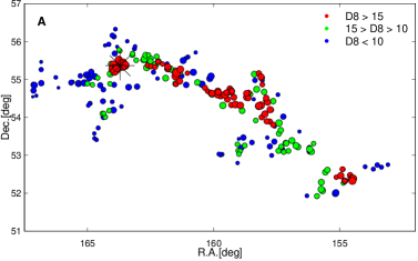
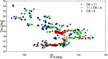
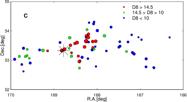
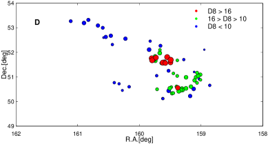
Figure 1: Distribution of galaxies in the BGW superclusters in the sky plane (from up to down: the superclusters A, B, C, and D). Red circles denote groups in the regions of the highest global density in each supercluster; green circles correspond to groups with intermediate luminosity density, and blue circles correspond to groups with the lowest luminosity density, as shown in the panels. The density limits are chosen so that each density interval contains approximately one-third of the supercluster galaxies. Symbol sizes are proportional to the value of the density field at the location of a galaxy. The stars in the plots of superclusters A and C denote the location of the Planck clusters PSZ2 G151.62+54.78 (supercluster A), and PSZ2 G150.56+58.32 (supercluster C).

We used the data from the twelfth data release (DR12) of the SDSS (Alam et al. 2015; York et al. 2000) Baryon Oscillation Spectroscopic Survey (BOSS; Eisenstein et al. 2011; Bolton et al. 2012; Dawson et al. 2013). The BOSS data was published in the Data Release 8 (DR8; Aihara et al. 2011). From these data, we use the CMASS (constant mass) sample, which selects massive and luminous galaxies in the redshift range $0.43<z<0.7$, with the stellar masses approximately constant up to $z\sim 0.6$ (Maraston et al. 2013). This is the massive end of the red sequence. These are the most abundant galaxies at the high mass end ($M>10^{11}\leavevmode\nobreak\ M_{\odot}$) and they evolve passively over the CMASS redshift range (Montero-Dorta et al. 2014, 2016). For the details of our sample we refer the reader to Lietzen et al. (2016).

Galaxy superclusters were determined using the luminosity-density field following the same procedure that was used in Liivamägi et al. (2012). We weighted the luminosities of galaxies in the r-band to keep the mean density the same through the whole distance range, and then calculated the density field on a 3 $h^{-1}$Mpc grid with a 8 $h^{-1}$Mpc smoothing scale. The calculation of the luminosity-density field is described in Liivamägi et al. (2012) and Tempel et al. (2014).

Superclusters of galaxies were defined as connected volumes above a certain luminosity density threshold. Lietzen et al. (2016) analysed the properties of superclusters at a series of density thresholds. They found an unusually high overdensity at $D8=5$ level, in which at the density level $D8=6$ individual superclusters can be distinguished from each other. Therefore, the BGW superclusters were extracted as connected volumes above the density level $D8=6$ times the mean luminosity density ($\ell_{\mathrm{mean}}$ = 5$\cdot 10^{-4}$ $\frac{10^{10}h^{-2}L_{\odot}}{(h^{-1}\mathrm{Mpc})^{3}}$) of the CMASS sample (Lietzen et al. 2016).

The BGW consists of two very rich superclusters with the diameters of 186 $h^{-1}$Mpc (supercluster A) and 173 $h^{-1}$Mpc (supercluster B), and of two moderately large superclusters (superclusters C and D) with the diameters of 64 and 91 $h^{-1}$Mpc. Data concerning the BGW superclusters are given in Table 1 which presents the number of galaxies in superclusters, the supercluster diameter (the maximum distance between the galaxies in the supercluster), the supercluster volume (the number of connected grid cells in the luminosity density field, multiplied by the cell volume), and the mean luminosity density in the supercluster, in units of the mean luminosity density. We show the sky distribution of galaxies in the BGW superclusters in Fig. 1. We plot galaxies in the high, medium, and low luminosity density regions in superclusters with different colours. Each region contains approximately one third of the supercluster galaxies. The full configuration of the BGW superclusters is shown in Lietzen et al. (2016).

We also used the data from the Second Planck Catalogue of Sunyaev-Zeldovich Sources (PSZ2) to identify Planck thermal Sunyaev-Zeldovich effect (tSZ) clusters in the BGW region (Planck Collaboration et al. 2015). Two Planck SZ sources were found: PSZ2 G150.56+58.32 in the region of the BGW supercluster C, and PSZ2 G151.62+54.78 in the region of the supercluster A. We show them in Fig. 1. These two Planck clusters correspond to the highest luminosity density of these individual superclusters.

Table 1: Data on the BGW superclusters.

ID	Richness	$\mathrm{Diameter}$	$\mathrm{Volume}$	$D8_{\mathrm{mean}}$
	$N_{\mathrm{gal}}$	$h^{-1}$Mpc	($h^{-1}$Mpc)3
A	255	186.1	67500	9.1
B	303	172.9	70848	9.3
C	73	63.8	19008	10.2
D	71	90.6	13635	9.3

3 Methods

3.1 Minkowski functionals and shapefinders

We employed the Minkowski functionals and shapefinders to study the morphology of the BGW superclusters. The BGW superclusters are defined as connected volumes above a certain luminosity density level, and can be characterised by their outer isodensity surface, and their enclosed volume. The morphology and topology of the isodensity contours are completely characterised by four Minkowski functionals. The Minkowski functionals were introduced in cosmology by Mecke et al. (1994). These functionals can be interpreted as the volume, the area, the integrated mean curvature (the first three Minkowski functionals), and the integrated Gaussian curvature (Euler characteristic) of the isodensity surface (the fourth Minkowski functional) (see Appendix A and Einasto et al. 2007b, 2011b, 2011c, for details and references). When increasing the isodensity level over the threshold overdensity, we move into the central parts of the supercluster. The Minkowski functionals can be calculated for the full range of density levels from the full supercluster to the central highest density peaks to show how the morphological properties of a supercluster change with the increase of the isodensity level.

Sahni et al. (1998) and Shandarin et al. (2004) used the first three Minkowski functionals to calculate the shapefinders $K_{1}$ (planarity) and $K_{2}$ (filamentarity), and their ratio, the shape parameter $K_{1}$/$K_{2}$ for the enclosed volume (see also Saar 2009). The smaller the shape parameter, the more elongated a supercluster is. The characteristic curve in the shapefinders $K_{1}$–$K_{2}$ plane is called the morphological signature (Einasto et al. 2007b). In the $K_{1}$/$K_{2}$-plane filaments are located near the $K_{2}$-axis and pancakes are located near the $K_{1}$-axis. Spheres are located at the origin of the plane where $K_{1}=K_{2}=0$, and ribbons along the diagonal of the plane.

The fourth Minkowski functional, $V_{3}$ (clumpiness), characterises the inner structure of superclusters. It shows the number of isolated clumps, void bubbles, and tunnels in the enclosed volume. When we increase the density level, the number of isolated clumps in a supercluster changes, void bubbles, and tunnels may appear inside a supercluster, and this changes the value of $V_{3}$. The higher the value of $V_{3}$, the more complicated is the inner morphology of the supercluster.

3.2 Principal component analysis and luminosity of superclusters from scaling relation

Einasto et al. (2011a) employed principal component analysis (PCA) to study the correlations between the physical and morphological properties of galaxy superclusters drawn from the SDSS DR7 and to determine scaling relations for superclusters. Principal component analysis finds a small number of linear combinations of correlated parameters to describe most of the variation in the dataset with a small number of new uncorrelated parameters. PCA transforms the data to a new Cartesian coordinate system, where the greatest variance by any projection of the data lies along the first coordinate (the first principal component), the second greatest variance – along the second coordinate, and so on. There are as many principal components as there are parameters, but typically only the first few are needed to explain most of the total variation. The principal components PC$x$ ($x\in\mathbb{N}$, $x\leq N_{\mathrm{tot}})$ are linear combinations of the original parameters:

$$PCx=\sum_{i=1}^{N_{\mathrm{tot}}}a_{x}(i)V_{i},$$ (1)

where $-1\leq a(i)_{x}\leq 1$ are the coefficients of the linear transformation, $V_{i}$ are the original parameters and $N_{\mathrm{tot}}$ is the number of the original parameters.

Efstathiou & Fall (1984) showed how to use PCA to get scaling relations. If, for example, the data points lie mostly along a plane, defined by the first two principal components, then the scaling relations for this plane are defined by the fact that the plane is perpendicular to the third principal component. In general, if the data dimension is higher, the points may be concentrated around a hyperplane that is perpendicular to the principal component $PCy$ that we choose to ignore in the total variance:

$$\sum_{i=1}^{N_{\mathrm{tot}}}a_{y}(i)\frac{(V_{i}-\overline{V_{i}})}{\sigma(V_{i})}=0.$$ (2)

Einasto et al. (2011a) studied the properties of galaxy superclusters with principal component analysis and found that superclusters can be characterised by a small number of physical and morphological parameters, the diameter and shape parameters among them. They derived the scaling relations for superclusters combining their morphological and physical parameters and showed that luminous superclusters can be divided into more elongated and less elongated systems, with different scaling relations. For elongated luminous superclusters the scaling relation from Einasto et al. (2011a) is:

$$\log(L)=(0.22K_{2}-1.67K_{1}+1.45)\cdot\log(D)+0.69,$$ (3)

where $L$ is the total luminosity of the supercluster (in units of $10^{10}L_{\odot}$, $D$ is the supercluster diameter (in units of $\mathrm{Mpc}/h$), and $K_{1}$ and $K_{2}$ are the shapefinders (planarity and filamentarity) for the supercluster. We found the morphological parameters for the BGW superclusters and then applied this scaling relation to calculate supercluster luminosities in r-band, denoted as $L^{\mathrm{scaling}}_{\mathrm{scl}}$. We also calculated the masses of superclusters using their luminosities from scaling relation, $L^{\mathrm{scaling}}_{\mathrm{scl}}$, and the mass-to-luminosity ratio as found for local rich superclusters in the r-band (Einasto et al. 2015, 2016), $M/L\approx 300$ $h\,M_{\odot}$/$L_{\odot}$. We denote the mass calculated in this way as $M^{\mathrm{scaling}}_{\mathrm{scl}}$.

3.3 Masses and luminosities of the BGW superclusters from stellar masses of galaxies

To estimate the minimum masses of the BGW superclusters we adopted the same procedure as in Lietzen et al. (2016) who used the stellar masses of galaxies to find the masses of the BGW superclusters. The BOSS stellar masses are obtained from the Portsmouth galaxy product (Maraston et al. 2013), which is based on the stellar population models by Maraston (2005) and Maraston et al. (2009). The Portsmouth product uses an adaptation of the publicly-available Hyper-Z code (Bolzonella et al. 2000) to perform a best-fit to the observed ugriz magnitudes of BOSS galaxies, with the spectroscopic redshift determined by the BOSS pipeline. The stellar masses used in this work were computed assuming the Kroupa initial mass function.

The virial masses of the host haloes of galaxies can be calculated from the relation between the stellar masses of the first ranked galaxies in haloes, $M_{*}$, and the virial masses of the haloes to which these galaxies belong, $M_{\mathrm{halo}}$ (Moster et al. 2010):

$$\frac{M_{*}}{M_{\mathrm{halo}}}=2\left(\frac{M_{*}}{M_{\mathrm{halo}}}\right)_{0}\left[\left(\frac{M_{\mathrm{halo}}}{M_{1}}\right)^{-\beta}+\left(\frac{M_{\mathrm{halo}}}{M_{1}}\right)^{\gamma}\right]^{-1},$$ (4)

where $(M_{*}/M_{\mathrm{halo}})_{0}=0.0254$ is the normalization of the stellar to halo mass relation, $M_{1}=10^{11.95}$ is a characteristic mass, and $\beta=1.37$ and $\gamma=0.55$ are the slopes of the low and high mass ends of the relation, respectively (Moster et al. 2010, Table 6). The sum of the halo masses gives us an estimate of the lower limit of the supercluster mass.

In calculations of the masses of superclusters we only used galaxies with stellar masses $\log(M_{*}/h^{-1}M_{\odot})\geq 11.3$, this is the completeness limit of the CMASS sample (Maraston et al. 2013). We assumed that galaxies in the CMASS sample with $\log(M_{*}/h^{-1}M_{\odot})\geq 11.3$ are the central galaxies of haloes. This is based on comparison with the Sloan Digital Sky Survey main sample of galaxies as follows. We used the magnitude-limited friend-of-friends group catalogue from the SDSS DR10 main sample by Tempel et al. (2014) to select galaxies in superclusters with the luminosity density $D8\geq 5$ in the distance bin from 180 to 270 $h^{-1}$Mpc. From this sample we determined a BOSS CMASS-like high-mass sample of galaxies with a stellar mass limit of $\log(M_{*}/h^{-1}M_{\odot})\geq 11.3$ and found that 87 % of all galaxies in this high-mass sample are the most luminous (first-ranked) galaxies in the friend-of-friends groups, or they are single galaxies (the main galaxies of faint groups, with satellite galaxies too faint to be observed in the SDSS). Therefore, we can assume that the high-mass galaxies in the BOSS sample are the first-ranked galaxies in groups. Comparison with local galaxies suggests that this may introduce an error in mass estimates of the order of about 10–15 %, considering that some massive galaxies may be members of the same group and not the main galaxies of different groups.

There are also haloes with the first-ranked galaxies having lower stellar masses than the limit $\log(M_{*}/h^{-1}M_{\odot})=11.3$. To take into account the mass in these haloes, we applied the scaling based on the analysis of the Sloan Digital Sky Survey main sample of galaxies. We again used the data about galaxies in superclusters with the luminosity density $D8\geq 5$ in the distance bin from 180 to 270 $h^{-1}$Mpc, and found that the ratio between the total stellar mass in high-mass galaxies and the total stellar mass in all first-ranked galaxies in the SDSS superclusters is 0.082 ($\approx 12$). The stellar masses of galaxies and halo masses are well correlated (Moster et al. 2010). Therefore we used this ratio to scale our minimum supercluster mass estimates. Our mass estimates differ from what was adopted in Lietzen et al. (2016) who used all galaxies in the BGW superclusters as the first-ranked galaxies in calculations of halo masses. For details we refer to Lietzen et al. (2016). We denote supercluster masses obtained from stellar masses of galaxies as $M^{\mathrm{*}}_{\mathrm{scl}}$.

We also calculated the luminosities of superclusters as the sum of the observed luminosities of high stellar mass galaxies in the r-band with a stellar mass limit of $\log(M_{*}/h^{-1}M_{\odot})\geq 11.3$ as in calculations of masses of superclusters. To take into account the luminosities of galaxies fainter than this limit we used the ratio of the mean luminosity density in the CMASS sample and the mean luminosity density of the SDSS MAIN galaxy sample ($\ell_{\mathrm{mean}}$ = 1.65$\cdot 10^{-2}$ $\frac{10^{10}h^{-2}L_{\odot}}{(h^{-1}\mathrm{Mpc})^{3}}$, see Liivamägi et al. 2012), corrected for the mean overdensity in the BGW region. These luminosities are denoted as $L^{\mathrm{lum}}_{\mathrm{scl}}$.

Below we calculate mass-to-light ratios $M^{\mathrm{*}}_{\mathrm{scl}}/L^{\mathrm{scaling}}_{\mathrm{scl}}$ for superclusters as the ratio of the mass obtained from the stellar masses of galaxies, and the luminosity of superclusters from the scaling relation. As input, the scaling relation uses morphological parameters of superclusters and supercluster diameters, being independent from other luminosity estimates that use galaxy luminosities. We also compare the luminosities and masses of superclusters obtained with two different methods.

4 Results

4.1 Morphology

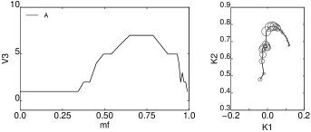
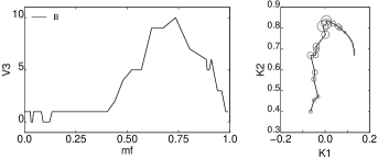
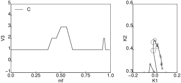
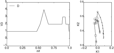
Figure 2: Left panels: the fourth Minkowski functional $V_{3}$ versus the mass fraction $mf$ for the BGW superclusters. Right panels: the shapefinders $K_{1}$ (planarity) and $K_{2}$ (filamentarity) plane for a supercluster. The morphological signature in the $K_{1}-K_{2}$ plane is parametrically defined as $K_{1}(mf)$ and $K_{2}(mf)$. The right-hand end of the $K_{1}$-$K_{2}$ curve corresponds to the whole supercluster (the mass fraction $mf=0$); the mass fraction increases counterclockwise along the $K_{1}-K_{2}$ curve. The sizes of open circles are proportional to the value of $V_{3}$ at a given mass fraction $mf$. They show the change of the clumpiness with the mass fraction together with the changes in the morphological signature. See text for more details.

Table 2: Morphological parameters for the BGW superclusters.

ID	Richness	diameter	$V_{3}$	$K_{1}$	$K_{2}$	$K_{1}$/$K_{2}$
		$h^{-1}$Mpc
A	255	186.1	7	0.12	0.68	0.17
B	303	172.9	10	0.13	0.67	0.19
C	73	63.8	4	0.07	0.32	0.21
D	71	90.6	3	0.08	0.35	0.24

Table 3: Luminosities, masses, and mass-to-light ratios of the BGW superclusters.

ID	$L^{\mathrm{lum}}_{\mathrm{scl}}$	$L^{\mathrm{scaling}}_{\mathrm{scl}}$	$M^{\mathrm{*}}_{\mathrm{scl}}$	$M^{\mathrm{*}}_{\mathrm{scl}}/L^{\mathrm{scaling}}_{\mathrm{scl}}$	$M^{\mathrm{scaling}}_{\mathrm{scl}}$
	$10^{12}h^{-2}L_{\sun}$	$10^{12}h^{-2}L_{\sun}$	$10^{16}h^{-1}M_{\odot}$	$h\,M_{\odot}$/$L_{\odot}$	$10^{16}h^{-1}M_{\odot}$
A	82.1	75.9	2.1	277	2.3
B	47.9	60.3	1.1	182	1.8
C	28.7	17.2	0.7	407	0.6
D	10.9	25.4	0.3	118	0.8
BGW	169.6	178.4	4.2	234	5.3

In Fig. 2 we present the fourth Minkowski functionals $V_{3}$ and the morphological signatures for the BGW superclusters. The values of the morphological parameters are given in Table 2. For the argument labelling the isodensity surfaces in Fig. 2 (left panels) we use the (excluded) mass fraction $mf$ – the ratio of the mass in the regions with lower density than at the isodensity surface, to the total mass of the supercluster. For the whole supercluster $mf=0$, this corresponds to the lowest value of the threshold density used to determine the supercluster. The mass fraction $mf=1$ corresponds to the peak density in the supercluster high-density cores. The fourth Minkowski functional $V_{3}$ is calculated for a full range of mass fractions from $mf=0$ to $mf=1$.

Figure 2 shows that at the mass fraction $mf\approx 0.3$, where approximately one third of galaxies from the outskirts of the supercluster do not contribute to the supercluster, the value of $V_{3}$ starts to increase. These outskirts regions are plotted in Fig. 1. At higher values of $mf$ superclusters become clumpy, they may split into several high-density cores, and may have void bubbles or tunnels in them. At a certain $mf$ level the value of $V_{3}$ reaches maximum. For rich BGW superclusters this happens at approximately $mf=0.7$ (Fig. 2), similarly to the local rich superclusters (Einasto et al. 2007b, 2011b). This mass fraction approximately marks the crossover from the lower density outskirts of the superclusters to the high-density cores. The galaxies in the high-density cores of the BGW superclusters are plotted in Fig. 1, where we give also the density levels which approximately correspond to $mf=0.7$. The BGW superclusters A and B have higher values of $V_{3}$ ($7$ and $10$), showing that they have a more complicated and richer inner structure than the BGW superclusters C and D (with $V_{3}=4$ and $3$). The clumpiness of the largest BGW supercluster (A) is lower than the clumpiness of the second largest supercluster. This may be due to a very high density core region of the A supercluster, which has a smaller number of individual clumps than the core region of the B supercluster. For poor BGW superclusters the maximum of $V_{3}$ occurs at a slightly lower $mf$ level. At still higher density levels less and less galaxies contribute to the superclusters and the value of the clumpiness $V_{3}$ decreases. High peaks in the $V_{3}$ distribution at high mass fractions for poor BGW superclusters suggest that they have high-density compact clumps in core regions. In the supercluster C one of these clumps corresponds to the Planck cluster PSZ2 G150.56+58.32. At high density levels the supercluster D splits into two parts, and the $V_{3}$ value decreases to two and increases again at very high density levels.

The richest local superclusters in the Sloan Great Wall (SGW) have maximum values of the clumpiness $V_{3}=13$ (the richest SGW supercluster) and $6$ (the second richest SGW supercluster), close to the $V_{3}$ values of the rich BGW superclusters (Einasto et al. 2011b). These superclusters contain several high-density cores, as the high $V_{3}$ values suggest also for the rich BGW superclusters (Einasto et al. 2016). The BGW supercluster C can be compared with the local A2142 supercluster which also has one very rich galaxy cluster in its main body, but morphologically the A2142 is different, it consists of one rich straight chain of galaxy groups and clusters (Einasto et al. 2015).

The right panels of Fig. 2 show how the morphological signatures of superclusters change with the mass fraction. The planarity $K_{1}$ has its maximum value at $mf=0$. When the mass fraction increases, the planarity $K_{1}$ of a supercluster decreases and the filamentarity $K_{2}$ increases (counterclockwise from right to left in the right panels of Fig. 2). The changes in the filamentarity $K_{2}$ at low mass fractions are more rapid than the changes in the planarity $K_{1}$, showing that superclusters become more elongated. At the mass fraction of about $mf=0.7$, the filamentarity $K_{2}$ reaches a maximum and then decreases showing that in the high-density cores where approximately one-third of supercluster galaxies reside, the morphology of a supercluster changes. The filamentarity $K_{2}$ decreases rapidly, and the planarity $K_{1}$ also decreases slightly. In this respect the BGW superclusters are similar to the richest local superclusters (Einasto et al. 2007b, 2011b). At high density levels at which the supercluster D divides into two, the morphological signature changes rapidly, too.

The largest difference between the local superclusters and the BGW superclusters is their overall shape - the BGW superclusters are very elongated, having lower shape parameter values for the whole superclusters than any local supercluster studied so far ($<0.25$ versus $>0.25$ for local rich superclusters, Einasto et al. 2011b).

4.2 The luminosities of superclusters

In Table 3 we show the luminosities of the BGW superclusters obtained using the luminosities of high stellar mass galaxies, as described in Sect. 3.3. For comparison, we also present the luminosities obtained by the scaling relation (Eq. (3)). This relation uses the data about supercluster diameters and shapefinders (Tables 1-3). Table 3 shows that the values of luminosities from two methods agree well, within 20% for rich BGW superclusters, and up to 2.7 times for poor BGW superclusters.

We can compare the luminosities of the BGW superclusters with the luminosities of superclusters from the SDSS by Liivamägi et al. (2012), (see also Einasto et al. 2012, 2016). The most luminous local superclusters are the richest SGW superclusters, with the luminosities $51.6\times 10^{12}h^{-2}L_{\sun}$ for the richest supercluster, and $29.2\times 10^{12}h^{-2}L_{\sun}$ for the second richest supercluster. Table 3 shows that the luminosity of the BGW A supercluster is almost equal to the sum of the luminosities of the two richest SGW superclusters. The BGW A supercluster is as large as these superclusters together therefore this result suggests that our methods to calculate the BGW supercluster luminosities work reasonably well.

4.3 The masses and mass-to-light ratios of the BGW superclusters

To find supercluster masses from the stellar masses of galaxies in superclusters we used the relation between stellar masses of galaxies and halo masses, as described in Sect. 3.3. The sum of halo masses was corrected for masses of missing haloes. The masses of superclusters, $M^{\mathrm{*}}_{\mathrm{scl}}$, are given in Table 3.

The mass of the second largest supercluster (B) in the BGW is approximatey half of the mass of the largest supercluster (A). This is because in this supercluster there are less very high stellar mass galaxies than in the supercluster A. Also Lietzen et al. (2016) noted that the stellar masses of the superclusters A and B are different with a high significance. The highest mass halo in the supercluster C can be identified with the Planck cluster PSZ2 G150.56+58.32 with the mass of $M\approx 7.6\times\leavevmode\nobreak\ 10^{14}h^{-1}M_{\odot}$ (Planck Collaboration et al. 2015). This makes the mass of this supercluster more than two times higher than the mass of another poor BGW supercluster D. Among Planck clusters in the BGW redshift range, $0.47\pm 0.05$, this cluster has the highest estimated mass. The mass of the lowest mass BGW supercluster D is similar to the mass of another supercluster at redshift $z\approx 0.5$, the SCL2243-0935 supercluster (Schirmer et al. 2011). The second Planck cluster, PSZ2 G151.62+54.78 in the supercluster A, is less massive with $M\approx 5.4\times\leavevmode\nobreak\ 10^{14}h^{-1}M_{\odot}$.

In Table 3 we also present supercluster masses obtained from their luminosities, estimated by the scaling relation. These two mass estimates coincide best for the BGW superclusters A and C. For superclusters B and D the difference between the two mass estimates is larger.

Einasto et al. (2016) estimated the masses of the SGW superclusters using several methods. The richest SGW supercluster has the total mass of about $1.2-1.4\times\leavevmode\nobreak\ 10^{16}h^{-1}M_{\odot}$. The mass range of other SGW superclusters and some other local superclusters is of about $0.3-0.7\times\leavevmode\nobreak\ 10^{16}h^{-1}M_{\odot}$ (Einasto et al. 2015, 2016). Thus the BGW supercluster A has a higher mass than very rich superclusters in the richest local galaxy system. The masses of other BGW superclusters are in the same range as the masses of rich local superclusters. We note that superclusters contain also intracluster gas. Therefore the BGW superclusters masses obtained by us in this work are the lower mass limits only.

We also present in Table 3 the mass-to-light ratios $M^{\mathrm{*}}_{\mathrm{scl}}/L^{\mathrm{scaling}}_{\mathrm{scl}}$ for the BGW superclusters, calculated using the luminosity of superclusters as obtained from the scaling relation (Eq. 3), and mass from stellar masses of galaxies. The values of the $M^{\mathrm{*}}_{\mathrm{scl}}/L^{\mathrm{scaling}}_{\mathrm{scl}}$ ratios for the largest BGW supercluster, $M/L=277$ and $182$ $h\,M_{\odot}$/$L_{\odot}$, are close to the values of the mass-to-light ratios of the largest two SGW superclusters, determined in the r-band, $M/L=271$ and $241$ $h\,M_{\odot}$/$L_{\odot}$ (Einasto et al. 2016). The $M^{\mathrm{*}}_{\mathrm{scl}}/L^{\mathrm{scaling}}_{\mathrm{scl}}$ ratio of the whole BGW is close to the value of the $M/L$ of the whole SGW, $234$ and $272$, correspondingly. The supercluster B has $M^{\mathrm{*}}_{\mathrm{scl}}/L^{\mathrm{scaling}}_{\mathrm{scl}}\approx 200$ $h\,M_{\odot}$/$L_{\odot}$. The same value of the mass-to-light ratio was obtained for the A901/902 supercluster at redshift $z=0.165$ in the r-band (Heymans et al. 2008). For the poor supercluster D we obtained the mass-to-light ratio $118$ $h\,M_{\odot}$/$L_{\odot}$. This is similar to the $M/L$ of the galaxy filaments in the SCL2243-0935 supercluster (Schirmer et al. 2011, in this paper the luminosities have been found in the i-band).

4.4 The uncertainties of morphology, luminosities and masses of the BGW superclusters

Morphological parameters. Uncertainties in calculation of the morphological parameters of superclusters come from how precicely we can calculate their values at low mass fractions, and from the choice of the density level used to define superclusters. We estimated that the uncertainties of the shapefinders $K_{1}$ and $K_{2}$ at low mass fractions are of the order of less than 5%. The superclusters were determined at fixed luminosity density level. If we decrease the density level used to define superclusters, new galaxies may be added to superclusters. Therefore, new clumps may appear at the outskirts of superclusters which may change the value of the fourth Minkowski functional $V_{3}$ at low mass fractions. The possible change in the morphological parameters is individual for each supercluster as discussed also in Einasto et al. (2011b). The BGW superclusters form a complex with overall very high luminosity density. The individual BGW superclusters were determined at the luminosity density level $D8=6$. Already at the density level $D8=5.5$ superclusters A and C, and superclusters B and D join to form two systems, and at $D8=5$ they join into one huge system (see Lietzen et al. 2016, for details). These systems have a clumpiness and overall shape which differ from those of individual superclusters, and cannot be compared with the MFs of individual superclusters. Einasto et al. (2011c) showed that at lower density levels at which the SGW superclusters join into huge systems the clumpiness and the shape parameter values increase, and that joint systems are more planar than the individual SGW superclusters.

Luminosity of superclusters. The errors in the luminosity obtained with Eq. (3) are related to how precicely we can calculate the values of the shapefinders $K_{1}$ and $K_{2}$. As we showed above these uncertainties are of the order of less than 5%. These errors cause approximately 1% uncertainty in luminosity, calculated using Eq. (3). This agrees with Einasto et al. (2011a), who showed that the PCA results for superclusters depend only very weakly on the choice of the density level used to define the superclusters. Another source of uncertainty comes from diameter errors. The diameter of a supercluster is defined as the maximum distance between supercluster galaxies. The main uncertainty of diameters is related to how robust is the supercluster definition using a fixed luminosity density level. If we decrease the density level, the superclusters A and C, and superclusters B and D join to form two systems, but no new galaxies join superclusters A, C, and D at their farthest edges where they could increase the diameter. The supercluster B has two galaxies added in one edge, the maximum increase in diameter is approximately $8$ $h^{-1}$ Mpc which leads to the 5% uncertainty in the luminosity of the supercluster.

The main source of uncertainty in luminosity calculations using the luminosity of massive galaxies comes from unobserved galaxies in the BGW superclusters. For the BGW A supercluster, our luminosity estimates have closer values than for the BGW B supercluster. It is possible that the galaxy content of the BGW superclusters A and B is different, with B containing relatively more faint galaxies. Lietzen et al. (2016) showed that the distribution of galaxy stellar masses in these superclusters is different, hinting that their galaxy content differ. The luminosities obtained by the two methods for poor superclusters differ up to 2.5 times, showing that the uncertainties are higher for poorer superclusters. We emphasise that when estimating supercluster luminosities by the scaling relation we used data about the diameter and shape parameters of superclusters. Even so, the values of luminosities obtained with two different methods are in good agreement, suggesting that uncertainties from unobserved galaxies in calculations of supercluster luminosities using galaxy luminosities, $L^{\mathrm{lum}}_{\mathrm{scl}}$, were taken into account correctly.

Masses of superclusters. The errors of supercluster masses were estimated using the stellar mass error estimates from Maraston et al. (2013) who found that the average errors of $\log(M_{*}/M_{\odot})$ are 0.1 dex. We recalculated the supercluster masses 1000 times using up to 0.1 dex random deviations of galaxy stellar mass values (assuming the Gaussian distribution of errors) in the calculations of halo masses. This gives $1\sigma$ errors of masses for the two richer superclusters as 0.05 and 0.06 dex, and for the superclusters C and D as 0.1 dex. After correcting for faint galaxies (Sect. 3.3, approximately 12 times) we find that the uncertainties in supercluster total mass estimates are of the order up to 15%.

5 Discussion and conclusions

Supercluster shape parameters. Our study of the morphology of the BGW superclusters showed that they are very elongated systems. The overall morphology of the BGW superclusters is similar to the morphology of local superclusters, with the maximum values of the fourth Minkowski functional $V_{3}$ up to 10. However, the BGW superclusters are more elongated, with the lower value of the shape parameter than local superclusters, $K1/K2<0.2$.

Einasto et al. (2007a) found that the richest superclusters from observations and simulations have the shape parameters $K1/K2>0.2$, similar results were obtained in Costa-Duarte et al. (2011). We use the CMASS luminous red galaxy data to trace the BGW superclusters, and owing to the morphology-density relation one might expect that luminous red galaxies trace the inner parts of superclusters only, making them to appear more elongated than they really are. For the local superclusters we can compare the Minkowski functionals and shapefinders for different galaxy populations (Einasto et al. 2008). This comparison showed that the Minkowski functionals and shapefinders for bright and faint, and for elliptical and spiral galaxies for the richest local superclusters in the outskirts of superclusters have similar values. Therefore we cannot conclude that very elongated shapes of the BGW superclusters are related to the use of the data for red galaxies only.

Another possible reason for the difference between the morphology of the BGW superclusters and the richest local superclusters may be related to the evolution of supercluster morphology. Araya-Melo et al. (2009) analysed the future evolution of galaxy superclusters in an acceleratingly expanding Universe and showed that in the future, superclusters will separate from each other and become less elongated. However, the redshift difference between the local supercluster sample and the BGW superclusters is not large ( 0.1 and 0.5) and it is questionable whether we should expect strong morphology evolution in this interval. To understand this, a study of supercluster morphology in a wide redshift interval is needed.

Supercluster masses, luminosities and mass-to-light ratios. We determined the luminosities and masses of the BGW superclusters with two methods, using the luminosities of high stellar mass galaxies in superclusters, corrected for the faint galaxies missing from the survey, and employing the morphological parameters filamentarity and planarity, and the diameters of superclusters. The values of luminosities and masses agree within approximately 20% for rich BGW superclusters, and up to 2.7 times for poor BGW superclusters suggesting that uncertainties in luminosity and mass calculations were taken into account properly.

We may expect that the BGW superclusters have higher luminosities than local superclusters of similar richness: the luminosity evolution of stellar populations of galaxies implies a $\approx 0.5-0.7$ mag dimming in the $r$-band, depending on the absolute age assumed as $z\approx 0.5$ (Maraston 2005; Montero-Dorta et al. 2016). However, we need to study a larger sample of superclusters to understand the evolutionary trends of supercluster properties.

We compare the masses of the richest BGW superclusters with the masses of the superclusters from the SGW below. The mass of the BGW supercluster C is dominated by a Planck cluster with the mass of $M\approx 7.6\times\leavevmode\nobreak\ 10^{14}h^{-1}M_{\odot}$; this is approximately one-tenth of the total mass of the supercluster according to our mass estimate. For comparison we mention that in the supercluster A2142 approximately one-fifth of the supercluster mass comes from the mass of a very rich galaxy cluster A2142 (Einasto et al. 2015). The values of the mass-to-luminosity ratios of the BGW superclusters are comparable to these of the local rich superclusters.

The BGW and SGW. The richest local supercluster complex is the SGW which has a total diameter of $230$ $h^{-1}$ Mpc, smaller than the BGW. The SGW consists of two rich and three poor superclusters (Einasto et al. 2016). These superclusters were defined as connected overdensity regions in the luminosity density field at the density level 5 (in units of the mean luminosity density). At a slightly lower density level, $4.7$, the superclusters from the SGW join into one huge system (Einasto et al. 2011c). This is similar to the BGW supercluster complex which forms one huge system at the luminosity density level 5 (Lietzen et al. 2016).

We showed that the clumpiness of the largest SGW supercluster is even higher than the clumpiness $V_{3}$ of the BGW supercluster A (13 vs. 10), which shows that this supercluster has a more complicated inner structure than the BGW A supercluster. The second richest superclusters in the BGW and the SGW have close $V_{3}$ values (7 and 6). The largest difference between the morphology of the BGW and SGW superclusters is that the BGW superclusters are very elongated, having shape parameter values $K_{1}/K_{2}<0.20$ while for the richest SGW superclusters $K_{1}/K_{2}=0.28$ and $0.48$ (Einasto et al. 2011b).

The comparison of the masses of the BGW superclusters with the masses of superclusters from the SGW shows that the most massive BGW supercluster (A) has a higher mass than any SGW supercluster (see Einasto et al. 2016, for the masses of the SGW superclusters). Einasto et al. (2016) estimated that the lower mass limit of the SGW is $M=2.4\times\leavevmode\nobreak\ 10^{16}h^{-1}M_{\odot}$, which is comparable to the mass of the BGW supercluster A, $M\approx 2.1\times\leavevmode\nobreak\ 10^{16}h^{-1}M_{\odot}$, and approximately two times lower than the mass of the whole BGW, $M=4.2\times\leavevmode\nobreak\ 10^{16}h^{-1}M_{\odot}$.

Similarly, the most luminous BGW supercluster (A) has the luminosity comparable to the sum of luminosities of the richest two SGW superclusters. In addition, Einasto et al. (2016) estimated that the total luminosity of the SGW is approximately $0.9\times 10^{14}h^{-2}L_{\sun}$ while in this paper we obtained that the total luminosity of the BGW is twice as high, $1.8\times 10^{14}h^{-2}L_{\sun}$. This shows that the BGW supercluster complex is richer, more massive and larger than the richest supercluster complex in the local Universe, the SGW.

Supercluster complexes. Einasto et al. (2011b) used data on the galaxy superclusters derived from the SDSS MAIN data to describe the morphology and large-scale distribution of superclusters in the local Universe. They showed that at the distance interval of $210-260$ $h^{-1}$ Mpc superclusters form three chains, separated by voids. One chain is formed by the SGW, other chains are formed by the Bootes, the Ursa Major, and other rich superclusters. All of these superclusters are poorer than the superclusters in the BGW. The very rich Corona Borealis supercluster is located at the intersection of supercluster chains, and it is separated from the SGW by voids. Therefore we cannot consider this supercluster as a member of a common complex with the SGW. There are also other very rich superclusters in the local Universe, like the Shapley, the Horologium-Reticulum, the Sculptor and others, but they are not located close to each other and do not form supercluster complexes like the BGW or the SGW (Einasto et al. 1997; Fleenor et al. 2005; Proust et al. 2006; Luparello et al. 2011).

At redshifts of $0.5$ and higher, just a few superclusters have been found so far (Tanaka et al. 2007; Swinbank et al. 2007; Gilbank et al. 2008; Schirmer et al. 2011; Pompei et al. 2016). Kim et al. (2016) mention that a supercluster at the redshift $z=0.9$ may be embedded in a $\approx 100$ $h^{-1}$ Mpc overdense structure but no rich supercluster complexes have yet been found at so high redshifts.

Supercluster morphology: filaments and spiders. Rich superclusters show wide morphological variety in which Einasto et al. (2011b) determined two main morphological types: spiders and filaments. Filament-type superclusters have elongated main bodies that connect galaxy groups and clusters in superclusters. Spider-type superclusters are systems of one or several high-density clumps with a large number of outgoing filaments connecting them. Empirical models show that morphological signatures of rich superclusters correspond to the multibranching systems of filament and spider types; poor superclusters typically are of spider type with one rich cluster surrounded by outgoing galaxy chains (Einasto et al. 2007b). Einasto et al. (2011b) classified superclusters as filaments and spiders on the basis of their morphological information and visual appearance. The BGW superclusters can be classified as being of filament-type (perhaps the supercluster C with its rich cluster and outgoing galaxy chains can be classified as a spider-type supercluster). Simulations show that while the sizes of the richest observed and simulated superclusters are comparable (Park et al. 2012), the morphological variety of the observed superclusters is not recovered in simulations yet (Einasto et al. 2007b). In particular, very dense and large filament-type superclusters like the richest SGW and BGW superclusters were not found among the richest simulated superclusters (Einasto et al. 2007b). This shows the need to study the richest superclusters and their complexes from observations and simulations in combination with the analysis of supercluster morphologies.

Sheth & Diaferio (2011) applied extreme value statistics to show that the presence of such a massive and dense structure as the SGW is difficult to reconcile with the assumption of Gaussian initial conditions if $\sigma_{8}$ is less than 0.9. They mention that this tension can be reduced if this structure is the densest within the Hubble volume. However, the discovery of the BGW shows that even richer systems exist. In addition, Einasto et al. (2006) showed that the fraction of very luminous superclusters among the observed superclusters is higher than among simulated superclusters. The study of the properties and evolution of very rich superclusters and their complexes using simulations with very large volume may constrain the assumptions on initial conditions.

In summary, the analysis of the morphology and luminosity of the BGW superclusters shows that the BGW is a unique complex of very rich and luminous superclusters having a very elongated shape and a complicated inner structure. The search for and detailed study of the richest superclusters and their complexes from observations and simulations in combination with the analysis of supercluster morphologies help us to understand the properties of the cosmic web and to constrain initial conditions.

Appendix A Minkowski functionals and shapefinders

For a given surface the four Minkowski functionals (from the first to the fourth) are proportional to the enclosed volume $V$, the area of the surface $S$, the integrated mean curvature $C$, and the integrated Gaussian curvature $\chi$. Consider an excursion set $F_{\phi_{0}}$ of a field $\phi(\mathbf{x})$ (the set of all points where the density is higher than a given limit, $\phi(\mathbf{x}\geq\phi_{0}$)). Then, the first Minkowski functional is the volume of this region (the excursion set):

$$V_{0}(\phi_{0})=\int_{F_{\phi_{0}}}\mathrm{d}^{3}x\;.$$ (5)

The second Minkowski functional is proportional to the surface area of the boundary $\delta F_{\phi}$ of the excursion set:

$$V_{1}(\phi_{0})=\frac{1}{6}\int_{\delta F_{\phi_{0}}}\mathrm{d}S(\mathbf{x})\;.$$ (6)

The third Minkowski functional is proportional to the integrated mean curvature $C$ of the boundary:

$$V_{2}(\phi_{0})=\frac{1}{6\pi}\int_{\delta F_{\phi_{0}}}\left(\frac{1}{R_{1}(\mathbf{x})}+\frac{1}{R_{2}(\mathbf{x})}\right)\mathrm{d}S(\mathbf{x})\;,$$ (7)

where $R_{1}(\mathbf{x})$ and $R_{2}(\mathbf{x})$ are the principal radii of curvature of the boundary.

Sahni et al. (1998) and Shandarin et al. (2004) used the first three Minkowski functionals to define the shapefinders called as the thickness, the width, and the length as follows. The thickness $H_{1}=3V/S$, the width $H_{2}=S/C$, and the length $H_{3}=C/4\pi$. The shapefinders have dimensions of length and are normalised to give $H_{i}=R$ for a sphere of radius $R$. For smooth (ellipsoidal) surfaces, the shapefinders $H_{i}$ follow the inequalities $H_{1}\leq H_{2}\leq H_{3}$. Oblate ellipsoids (pancakes) are characterised by $H_{1}<<H_{2}\approx H_{3}$, while prolate ellipsoids (filaments) are described by $H_{1}\approx H_{2}<<H_{3}$.

Sahni et al. (1998) also defined two dimensionless shapefinders $K_{1}$ (planarity) and $K_{2}$ (filamentarity): $K_{1}=(H_{2}-H_{1})/(H_{2}+H_{1})$ and $K_{2}=(H_{3}-H_{2})/(H_{3}+H_{2})$. We use these shapefinders in our study to analyse the shape of the superclusters.

The fourth Minkowski functional is proportional to the integrated Gaussian curvature (the Euler characteristic) of the boundary:

$$V_{3}(\phi_{0})=\frac{1}{4\pi}\int_{\delta F_{\phi_{0}}}\frac{1}{R_{1}(\mathbf{x})R_{2}(\mathbf{x})}\mathrm{d}S(\mathbf{x})\;.$$ (8)

This functional describes the topology of the surface; it is a sum of the number of isolated clumps and the number of void bubbles minus the number of tunnels (voids open from both sides) in the region (see, e.g. Martínez & Saar 2002; Saar et al. 2007):

$$V_{3}=N_{\mathrm{clumps}}+N_{\mathrm{cavities}}-N_{\mathrm{tunnels}}.$$ (9)

High values of the fourth Minkowski functional $V_{3}$ suggest a complicated (clumpy) morphology of a supercluster.

References

- Aihara et al. (2011) Aihara, H., Allende Prieto, C., An, D., et al. 2011, ApJS, 193, 29
- Alam et al. (2015) Alam, S., Albareti, F. D., Allende Prieto, C., et al. 2015, ApJS, 219, 12
- Araya-Melo et al. (2009) Araya-Melo, P. A., Reisenegger, A., Meza, A., et al. 2009, MNRAS, 399, 97
- Basilakos (2003) Basilakos, S. 2003, MNRAS, 344, 602
- Bolton et al. (2012) Bolton, A. S., Schlegel, D. J., Aubourg, É., et al. 2012, AJ, 144, 144
- Bolzonella et al. (2000) Bolzonella, M., Miralles, J.-M., & Pelló, R. 2000, A&A, 363, 476
- Chow-Martínez et al. (2014) Chow-Martínez, M., Andernach, H., Caretta, C. A., & Trejo-Alonso, J. J. 2014, MNRAS, 445, 4073
- Costa-Duarte et al. (2011) Costa-Duarte, M. V., Sodré, Jr., L., & Durret, F. 2011, MNRAS, 411, 1716
- Dawson et al. (2013) Dawson, K. S., Schlegel, D. J., Ahn, C. P., et al. 2013, AJ, 145, 10
- de Vaucouleurs (1956) de Vaucouleurs, G. 1956, Vistas in Astronomy, 2, 1584
- Efstathiou & Fall (1984) Efstathiou, G. & Fall, S. M. 1984, MNRAS, 206, 453
- Einasto et al. (2006) Einasto, J., Einasto, M., Saar, E., et al. 2006, A&A, 459, L1
- Einasto et al. (2007a) Einasto, J., Einasto, M., Saar, E., et al. 2007a, A&A, 462, 397
- Einasto et al. (2015) Einasto, M., Gramann, M., Saar, E., et al. 2015, A&A, 580, A69
- Einasto et al. (2016) Einasto, M., Lietzen, H., Gramann, M., et al. 2016, A&A, 595, A70
- Einasto et al. (2014) Einasto, M., Lietzen, H., Tempel, E., et al. 2014, A&A, 562, A87
- Einasto et al. (2011a) Einasto, M., Liivamägi, L. J., Saar, E., et al. 2011a, A&A, 535, A36
- Einasto et al. (2011b) Einasto, M., Liivamägi, L. J., Tago, E., et al. 2011b, A&A, 532, A5
- Einasto et al. (2011c) Einasto, M., Liivamägi, L. J., Tempel, E., et al. 2011c, ApJ, 736, 51
- Einasto et al. (2012) Einasto, M., Liivamägi, L. J., Tempel, E., et al. 2012, A&A, 542, A36
- Einasto et al. (2007b) Einasto, M., Saar, E., Liivamägi, L. J., et al. 2007b, A&A, 476, 697
- Einasto et al. (2008) Einasto, M., Saar, E., Martínez, V. J., et al. 2008, ApJ, 685, 83
- Einasto et al. (1997) Einasto, M., Tago, E., Jaaniste, J., Einasto, J., & Andernach, H. 1997, A&AS, 123 [astro-ph/9610088]
- Eisenstein et al. (2011) Eisenstein, D. J., Weinberg, D. H., Agol, E., et al. 2011, AJ, 142, 72
- Fleenor et al. (2005) Fleenor, M. C., Rose, J. A., Christiansen, W. A., et al. 2005, AJ, 130, 957
- Geach et al. (2011) Geach, J. E., Ellis, R. S., Smail, I., Rawle, T. D., & Moran, S. M. 2011, MNRAS, 413, 177
- Gilbank et al. (2008) Gilbank, D. G., Yee, H. K. C., Ellingson, E., et al. 2008, ApJ, 677, L89
- Heymans et al. (2008) Heymans, C., Gray, M. E., Peng, C. Y., et al. 2008, MNRAS, 385, 1431
- Ihaka & Gentleman (1996) Ihaka, R. & Gentleman, R. 1996, Journal of Computational and Graphical Statistics, 5, 299
- Jõeveer et al. (1978) Jõeveer, M., Einasto, J., & Tago, E. 1978, MNRAS, 185, 357
- Kim et al. (2016) Kim, J.-W., Im, M., Lee, S.-K., et al. 2016, ApJ, 821, L10
- Kolokotronis et al. (2002) Kolokotronis, V., Basilakos, S., & Plionis, M. 2002, MNRAS, 331, 1020
- Komatsu et al. (2011) Komatsu, E., Smith, K. M., Dunkley, J., et al. 2011, ApJS, 192, 18
- Lietzen et al. (2012) Lietzen, H., Tempel, E., Heinämäki, P., et al. 2012, A&A, 545, A104
- Lietzen et al. (2016) Lietzen, H., Tempel, E., Liivamägi, L. J., et al. 2016, A&A, 588, L4
- Liivamägi et al. (2012) Liivamägi, L. J., Tempel, E., & Saar, E. 2012, A&A, 539, A80
- Lubin et al. (2009) Lubin, L. M., Gal, R. R., Lemaux, B. C., Kocevski, D. D., & Squires, G. K. 2009, AJ, 137, 4867
- Luparello et al. (2011) Luparello, H., Lares, M., Lambas, D. G., & Padilla, N. 2011, MNRAS, 415, 964
- Maraston (2005) Maraston, C. 2005, MNRAS, 362, 799
- Maraston et al. (2013) Maraston, C., Pforr, J., Henriques, B. M., et al. 2013, MNRAS, 435, 2764
- Maraston et al. (2009) Maraston, C., Strömbäck, G., Thomas, D., Wake, D. A., & Nichol, R. C. 2009, MNRAS, 394, L107
- Martínez & Saar (2002) Martínez, V. J. & Saar, E. 2002, Statistics of the Galaxy Distribution (Chapman & Hall/CRC, Boca Raton)
- Mecke et al. (1994) Mecke, K. R., Buchert, T., & Wagner, H. 1994, A&A, 288, 697
- Montero-Dorta et al. (2014) Montero-Dorta, A. D., Bolton, A. S., Brownstein, J. R., et al. 2014, ArXiv e-prints [arXiv:1410.5854]
- Montero-Dorta et al. (2016) Montero-Dorta, A. D., Shu, Y., Bolton, A. S., Brownstein, J. R., & Weiner, B. J. 2016, MNRAS, 456, 3265
- Moster et al. (2010) Moster, B. P., Somerville, R. S., Maulbetsch, C., et al. 2010, ApJ, 710, 903
- Park et al. (2012) Park, C., Choi, Y.-Y., Kim, J., et al. 2012, ApJ, 759, L7
- Planck Collaboration et al. (2015) Planck Collaboration, Ade, P. A. R., Aghanim, N., et al. 2015, ArXiv e-prints [arXiv:1502.01598]
- Pompei et al. (2016) Pompei, E., Adami, C., Eckert, D., et al. 2016, A&A, 592, A6
- Proust et al. (2006) Proust, D., Quintana, H., Carrasco, E. R., et al. 2006, A&A, 447, 133
- Reid et al. (2016) Reid, B., Ho, S., Padmanabhan, N., et al. 2016, MNRAS, 455, 1553
- Saar (2009) Saar, E. 2009, in Data Analysis in Cosmology, ed. V. J. Martínez & E. Saar & E. Martínez-Gonzalez & M.-J. Pons-Bordería (Springer-Verlag, Berlin), 523–563
- Saar et al. (2007) Saar, E., Martínez, V. J., Starck, J., & Donoho, D. L. 2007, MNRAS, 374, 1030
- Sahni et al. (1998) Sahni, V., Sathyaprakash, B. S., & Shandarin, S. F. 1998, ApJ, 495, L5
- Sathyaprakash et al. (1998) Sathyaprakash, B. S., Sahni, V., & Shandarin, S. 1998, ApJ, 508, 551
- Schirmer et al. (2011) Schirmer, M., Hildebrandt, H., Kuijken, K., & Erben, T. 2011, A&A, 532, A57
- Schmalzing & Buchert (1997) Schmalzing, J. & Buchert, T. 1997, ApJ, 482, L1
- Shandarin et al. (2004) Shandarin, S. F., Sheth, J. V., & Sahni, V. 2004, MNRAS, 353, 162
- Sheth et al. (2003) Sheth, J. V., Sahni, V., Shandarin, S. F., & Sathyaprakash, B. S. 2003, MNRAS, 343, 22
- Sheth & Diaferio (2011) Sheth, R. K. & Diaferio, A. 2011, MNRAS, 417, 2938
- Shim & Lee (2013) Shim, J. & Lee, J. 2013, ApJ, 777, 74
- Shim et al. (2014) Shim, J., Lee, J., & Baldi, M. 2014, ArXiv e-prints [arXiv:1404.3639]
- Swinbank et al. (2007) Swinbank, A. M., Edge, A. C., Smail, I., et al. 2007, MNRAS, 379, 1343
- Tanaka et al. (2007) Tanaka, M., Hoshi, T., Kodama, T., & Kashikawa, N. 2007, MNRAS, 379, 1546
- Tempel et al. (2009) Tempel, E., Einasto, J., Einasto, M., Saar, E., & Tago, E. 2009, A&A, 495, 37
- Tempel et al. (2011) Tempel, E., Saar, E., Liivamägi, L. J., et al. 2011, A&A, 529, A53
- Tempel et al. (2014) Tempel, E., Tamm, A., Gramann, M., et al. 2014, A&A, 566, A1
- York et al. (2000) York, D. G., Adelman, J., Anderson, Jr., J. E., et al. 2000, AJ, 120, 1579