An online slow manifold approach for efficient optimal control of multiple time-scale kinetics

Abstract

Chemical reactions modeled by ordinary differential equations are finite-dimensional dissipative dynamical systems with multiple time-scales. They are numerically hard to tackle – especially when they enter an optimal control problem as “infinite-dimensional” constraints. Since discretization of such problems usually results in high-dimensional nonlinear problems, model (order) reduction via slow manifold computation seems to be an attractive approach. We discuss the use of slow manifold computation methods in order to solve optimal control problems more efficiently having real-time applications in view.

1 Introduction

Chemical kinetics with multiple time scales and their control involve highly stiff and often high-dimensional ordinary differential equations (ODE). This poses hard challenges to the numerical solution and is the reason why model reduction methods are considered. The dynamics can be simplified by focusing on the long time behavior of such systems (leaving fast transients unresolved) and calculating fast modes as functions of the slow ones. Ideally this leads to low dimensional manifolds in high-dimensional state space. In the special case of singularly perturbed system, they are understood quite well and called slow invariant manifolds.

An open problem is how the slow manifolds can be used to simplify the solution of optimal control problems (OCP) that involve multiple time scale ODE constraints.

2 Slow Manifold Computation

In dissipative dynamical systems geometrically the bundling of trajectories (on a fast time scale) to low-dimensional manifolds is observed. Once trajectories reach the neighborhood of the slow manifold, they will evolve slowly and will never leave this manifold neighborhood. Thus, this manifold is called slow invariant attracting manifold (SIAM).

The aim of slow manifold computation techniques is to approximately compute the SIAM as the graph of a function of only a few selected species (so called reaction progress variables). Thus, manifold-based model reduction generate a function $h\mathrel{\mathop{\mathchar 58\relax}}\mathbb{R}^{n_{s}}\rightarrow\mathbb{R}^{n_{f}}$ ($n_{s}$ is the number of slow variables resp. reaction progress variables and $n_{f}$ is the number of fast variables), such that $\left(z_{s},h(z_{s})\right)$ approximates points of the SIAM.

In order to investigate optimal control benchmark problems, we consider singularly perturbed systems, i.e. systems where the ODE can be transformed into the following form:

$$\dot{z_{s}}(t) =f_{s}(z_{s}(t),z_{f}(t))$$ (1a)

$$\varepsilon\dot{z_{f}}(t) =f_{f}(z_{s}(t),z_{f}(t)).$$ (1b)

Two methods relevant in our context for the approximative calculation of the SIAM are briefly reviewed in the following subsections.

2.1 Zero Derivative Principle

The main idea of the Zero Derivative Principle (ZDP) [1],[6] for model reduction of singularly perturbed systems is to identify for given values of the slow variables $z_{s}^{*}$ a point $z_{f}^{*}$ such that the higher-order time derivatives of fast components vanish, i.e

$$\frac{\operatorname{d\!}{}^{m}f_{f}(z_{s}^{*},z_{f}^{*})}{\operatorname{d\!}t^{m}}=0\qquad\text{for a given }m\in\mathbb{N}.$$ (2)

2.2 Method of Lebiedz and Unger

Another approach proposed by Lebiedz and Unger [4] is motivated geometrically: Among arbitrary trajectories of (1) for which the slow components end within the time $t_{1}-t_{0}$ in the state $z_{s}^{*}$ the corresponding part of the trajectory on the SIAM is characterized by the smallest curvature (see also [2],[3]). This motivates optimization problem (3) which is a variational boundary value problem (BVP).

$$\min\limits_{z(\cdot)=\big{(}z_{s}(\cdot),z_{f}(\cdot)\big{)}}\quad \mathinner{\!\left\lVert\ddot{z}(t_{0})\right\rVert}_{2}^{2}$$ (3a)

s.t. $$\dot{z}_{s} =f_{s}\big{(}z_{s},z_{f}\big{)},\quad t\in[t_{0},t_{1}]$$ (3b)

$$\varepsilon\dot{z}_{f} =f_{f}\big{(}z_{s},z_{f}\big{)},\quad t\in[t_{0},t_{1}]$$ (3c)

$$z_{s}(t_{1}) =z_{s}^{*}.$$ (3d)

In our application context we also use the local reformulation of problem (3), where $t_{0}=t_{1}$.

3 Optimal Control

One of our research interests is to solve optimal control problems involving multiple time scales as it appears frequently e.g. in the field of chemical engineering. Thus, we consider the following (typically high-dimensional) OCP:

$$\quad\,\min_{z_{s},z_{f},u} \int_{0}^{T} L(z_{s},z_{f},u)\operatorname{d\!}t$$ (4a)

subject to $$\dot{z_{s}} =f_{s}(z_{s},z_{f},u)$$ (4b)

$$\varepsilon\dot{z_{f}} =f_{f}(z_{s},z_{f},u)$$ (4c)

$$z_{s}(0) =z_{s}^{(0)},\;z_{f}(0)=z_{f}^{(0)}$$ (4d)

Applying the model reduction methods presented in the last section and assuming the control $u$ to be a slow variable, yields the lower dimensional problem (cf. [5])

$$\quad\,\min_{z_{s},u} \int_{0}^{T} L(z_{s},h(z_{s},u),u)\operatorname{d\!}t$$ (5a)

subject to $$\dot{z_{s}} =f_{s}(z_{s},h(z_{s},u),u)$$ (5b)

$$z_{s}(0) =z_{s}^{(0)}.$$ (5c)

This systems has the advantage, that it has significantly less optimization variables and the ODE (5) is less stiff, which makes it solvable by fast explicit numerical integrators compared to implicit methods required for stiff ODE. However, numerical solution methods for OCPs like the multiple shooting method need repeated evaluation of the function $h$ as well as its partial derivatives $h_{z_{s}}$ and $h_{u}$.

Therefore, it would be beneficial to combine the calculation of the SIM and the optimal control problem. This is obviously possible, if the approximation $h(z_{s})$ of the SIM can be formulated as a (nonlinear) root finding problem $r(z_{s},z_{f},u)=0$, e.g. with the ZDP method. Thus, we propose to solve the following OCP instead of (5):

$$\quad\,\min_{z_{s},z_{f},u} \int_{0}^{T} L(z_{s},z_{f},u)\operatorname{d\!}t$$ (6a)

subject to $$\dot{z_{s}} =f_{s}(z_{s},z_{f},u)$$ (6b)

$$0 =r(z_{s},z_{f},u)$$ (6c)

$$z_{s}(0) =z_{s}^{(0)}.$$ (6d)

4 Application to Chemical Reactions

We apply the ideas presented in the last sections to a benchmark OCP motivated by the Michaelis-Menten-Henri mechanism

$$S+E\leftrightharpoons SE\rightarrow P+E,$$ (7)

modeling the reaction of substrate $S$ to a product $P$ via a substrate-enzyme-complex $SE$ with the help of enzyme $E$. Simplifying the ODE given by (7) and introducing an artificial objective function yields OCP (8).

$$\min_{z_{s},z_{f},u}\quad \int_{0}^{5}-50z_{f}+u^{2}\operatorname{d\!}t$$ (8a)

s.t. $$\begin{array}[]{rrrll}\dot{z_{s}}&=&-z_{s}&+\left(z_{s}+0.5\right)z_{f}+u,\\ \varepsilon\dot{z_{f}}&=&z_{s}&-\left(z_{s}+1\right)z_{f},\\ z_{s}(0)&=&1,&&\end{array}$$ (8e)

where the control $u(t)\in[0,10]$ represents the possibility to add some substrate (corresponds to variable $z_{s}$) to the system and $\varepsilon$ describes the time-scale separation (between the time evolution of $z_{s}$ and $z_{f}$).

Figure 1 shows the results of the numerical solution of (8) using the multiple-shooting scheme with an implicit Radau-2A integrator. If we refer to the solution of the proposed OCP (6) as $(z_{s}^{\text{app}},z_{f}^{\text{app}},u^{\text{app}})$ and to the solution of (8) as $(z_{s}^{\text{orig}},z_{f}^{\text{orig}},u^{\text{orig}})$, then it holds

$$\max\left\{\lvert\lvert z_{s}^{\text{orig}}-z_{s}^{\text{app}}\rvert\rvert_{\infty},\lvert\lvert z_{f}^{\text{orig}}-z_{f}^{\text{app}}\rvert\rvert_{\infty},\lvert\lvert u^{\text{orig}}-u^{\text{app}}\rvert\rvert_{\infty}\right\}$$

$$=\lvert\lvert z_{s}^{\text{orig}}-z_{s}^{\text{app}}\rvert\rvert_{\infty}\approx 0.05,$$ (9)

which gives a relative error of $\approx 0.2\%$ for both objective functional value and $\lvert\lvert z_{s}^{\text{orig}}-z_{s}^{\text{app}}\rvert\rvert_{\infty}/\lvert\lvert z_{s}^{\text{orig}}\rvert\rvert_{\infty}$. Although, the proposed method uses exactly as many variables than the original OCP, we observe a speed up of factor 4 for solving OCP (8) due to the use of an explicit integration scheme.

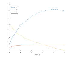
Figure 1: Numerical Solution of (8).

References

- [1] C. W. Gear and T. J. Kaper and I. G. Kevrekidis and A. Zagaris, Projecting to a Slow Manifold: Singularly Perturbed Systems and Legacy Codes, SIAM Journal on Applied Dynamical Systems, 4 (2005), pp. 711–732.
- [2] D. Lebiedz, Computing minimal entropy production trajectories: An approach to model reduction in chemical kinetics, Journal of Chemical Physics, 120 (2004), pp. 6890–6897.
- [3] D. Lebiedz, J. Siehr and J. Unger, A variational principle for computing slow invariant manifolds in dissipative dynamical systems, SIAM Journal on Scientific Computing, 33 (2011), pp. 703–720.
- [4] D. Lebiedz and J. Unger, On unifying concepts for trajectory-based slow invariant attracting manifold computation in kinetic multi-scale models, Mathematical and Computer Modelling of Dynamical Systems, 22 (2016), pp. 87–112.
- [5] M. Rehberg , A Numerical Approach to Model Reduction for Optimal Control of Multiscale ODE, PhD thesis, 2013.
- [6] A. Zagaris, C. W. Gear, T. J. Kaper and Y. G. Kevrekidis, Analysis of the accuracy and convergence of equation-free projection to a slow manifold, Mathematical Modelling and Numerical Analysis, 43 (2009), pp. 757–784.