Efficient regularization with wavelet sparsity constraints in PAT

Abstract

In this paper we consider the reconstruction problem of photoacoustic tomography (PAT) with a flat observation surface. We develop a direct reconstruction method that employs regularization with wavelet sparsity constraints. To that end, we derive a wavelet-vaguelette decomposition (WVD) for the PAT forward operator and a corresponding explicit reconstruction formula in the case of exact data. In the case of noisy data, we combine the WVD reconstruction formula with soft-thresholding which yields a spatially adaptive estimation method. We demonstrate that our method is statistically optimal for white random noise if the unknown function is assumed to lie in any Besov-ball. We present generalizations of this approach and, in particular, we discuss the combination of vaguelette soft-thresholding with a TV prior. We also provide an efficient implementation of the vaguelette transform that leads to fast image reconstruction algorithms supported by numerical results.

Key words: Photoacoustic tomography, image reconstruction, wavelet-vaguelette decomposition, variational regularization, sparsity constraints, wavelet-TV regularization.

AMS subject classification: 49N45, 65N21, 92C55.

1 Introduction

Photoacoustic tomography (PAT) is a novel coupled-physics (hybrid) modality for non-invasive biomedical imaging that combines the high contrast of optical tomography with the high spatial resolution of acoustic imaging [7, 65, 98, 95, 100]. Its principle consists in illuminating a sample by an electromagnetic pulse that, due to the photoacoustic effect, generates pressure waves inside of the object; see Figure 1. The generated pressure waves (the acoustic signals) then propagate through the sample and beyond, and the pressure is recorded outside of the sample. Finally, mathematical algorithms are used to reconstruct an image of the interior (see, for example, [66, 81, 100]).

In this paper we work with the standard model of PAT, where the acoustic pressure $u\colon\mathbb{R}^{d}\times\left(0,\infty\right)\to\mathbb{R}$ solves the standard wave equation (see (3)). The goal of PAT is to recover the initial pressure distribution (at time $t=0$), given by a function $h:\mathbb{R}^{d}\to\mathbb{R}$, from measurements $\mathbf{U}h\coloneqq u|_{\partial\mathbb{H}_{+}\times(0,\infty)}$ of the pressure that is recorded on the hyperplane $\partial\mathbb{H}_{+}$. Here, $\mathbb{H}_{+}$ denotes the half space $\mathbb{R}^{d-1}\times(0,\infty)$. That is, we assume that we know $u$ on $\partial\mathbb{H}_{+}=\mathbb{R}^{d-1}\times\{0\}$ (the acquisition surface), and our goal is to reconstruct $h$ from (possibly approximate) knowledge of $\mathbf{U}h$. This is an inverse problem, which amounts to an (approximate) inversion of the operator $\mathbf{U}$. We will refer to that problem as the inverse problem of PAT with a planar acquisition geometry. Note that similar approaches can be considered for other acquisition geometries as well.

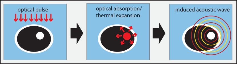
Figure 1: Basic principle of PAT. A semitransparent sample is illuminated with a short optical pulse. Due to optical absorption and subsequent thermal expansion an acoustic pressure wave is induced within the sample. The pressure waves are measured outside of the sample and used to reconstruct an image of the interior.

In the case of exact data $\mathbf{U}h$, several approaches have been derived for solving the inverse problem of PAT considering different acquisition geometries. This includes time reversal (see [16, 60, 39, 76, 92]), Fourier domain algorithms (see [59, 2, 68, 101, 64, 61, 13, 77, 36, 4]), analytic reconstruction formulas of back-projection type (see [79, 38, 39, 51, 53, 58, 67, 73, 99]), as well as iterative approaches [31, 57, 80, 82, 87, 102, 96, 97]. For the case of noisy data, it is well known that iterative methods (including variational methods and sparse reconstructions) tend to be more accurate than analytic methods.

Among those iterative techniques, sparse regularization approaches have gained a lot of attention during the last years as they have proven to perform well for noisy data as well as for incomplete data problems. One of their main advantages consists in their ability to combine efficient regularization with good feature preservation and to (to some extent) to compensate for the missing data [10, 44, 85, 54]. However, these advantages of sparse regularization methods come with the cost of typically significantly longer reconstruction times than FBP-type approaches. This is because the forward and adjoint operators have to be evaluated repeatedly. Due to that reason, FBP type methods (or other direct approaches) are often preferred over the more elaborate sparse regularization techniques [3, 5, 16, 83, 84].

In this paper we develop numerically efficient reconstruction method for PAT with planar geometry that effectively deals with noisy data $g=\mathbf{U}h+z$, where regularization is achieved by enforcing sparsity constraints in the reconstruction with respect to wavelet coefficients of $h$. More precisely, we derive a direct method for calculating a minimizer the $\ell^{1}$-Tikhonov functional

$$\boldsymbol{\Phi}_{g,w}(h)\coloneqq\frac{1}{2}\left\lVert\mathbf{U}h-g\right\rVert^{2}+\sum_{\lambda\in\Lambda}w_{\lambda}\left\lvert\left\langle\psi_{\lambda},h\right\rangle\right\rvert,$$ (1)

where $(\psi_{\lambda})_{\lambda\in\Lambda}$ denotes an orthonormal wavelet basis and $w_{\lambda}>0$ are weights. To achieve that, as one of our main results, we construct a wavelet-vaguelette decomposition for the operator $\mathbf{U}$. That is, given a wavelet basis $(\psi_{\lambda})_{\lambda\in\Lambda}$, we construct a system $(v_{\lambda})_{\lambda\in\Lambda}$ in $\mathrm{ran}\left(\mathbf{U}\right)$ that, in the case of exact data $g=\mathbf{U}h$, gives rise to an inversion formula of the form $h=\sum_{\lambda}\kappa_{\lambda}\langle\mathbf{U}h,v_{\lambda}\rangle\psi_{\lambda}$. Given noisy data $g=\mathbf{U}h+z$, we show that a combination of this formula with soft-thresholding $\mathbf{s}_{w}$, namely

$$h^{*}=\sum_{\lambda}\kappa_{\lambda}\,\mathbf{s}_{w}(\langle g,v_{\lambda}\rangle)\psi_{\lambda},$$ (2)

provides a minimizer of the functional (1). Additionally, we derive an efficient algorithm for the vaguelette transform $g\mapsto(\langle g,v_{\lambda}\rangle)_{\lambda}$ and provide an implementation for the WVD reconstruction (2). Moreover, we show order optimality of our method in the case of deterministic noise as well as is the case of Gaussian random noise. We also consider generalizations of our method and, in particular, we show how WVD reconstruction can be combined with an additional TV-prior.

Sparse regularization has been widely used as a reconstruction method for general inverse problems and there is a vast literature on that topic (see, for example, [14, 30, 40, 48, 49, 52, 69, 86, 88, 94]). In the statistical setting, $\ell^{1}$-Tikhonov regularization is known as LASSO [91, 11, 103, 78] or basis pursuit [22]. In most cases, the reconstructions are computed by employing iterative algorithms (such as iterative soft-thresholding) to minimize the $\ell^{1}$-Tikhonov functional [12, 26, 27, 30, 37, 8]. As mentioned above, those methods have the disadvantage to be slower than FBP type methods, as the forward and adjoint problem have to be solved repeatedly.

Wavelet-vaguelette decompositions and generalizations like biorthogonal curvelet decompositions and shearlet decompositions have been derived for the classical Radon transform in 2D, see [1, 33, 17, 25, 63]. To the best of our knowledge, this paper is the first to provide a WVD for photoacoustic tomography as well as an efficient direct implementation of sparse regularization using wavelets for that case.

Organization of the paper

In section 2 we review the mathematical principles of PAT with a flat observation surface and collect results required for our further analysis. In Section 3 we derive the WVD for the forward operator. The WVD is then used to define the soft-thresholding estimator in Section 4. In that section we also discuss the equivalence to variational estimation such as $\ell^{1}$-Tikhonov regularization. The efficient implementation of the estimator requires and efficient implementation of the vaguelette transform. Such an algorithm is derived in Section 5, where we also present results of our numerical simulation

2 PAT with a flat observation surface

Let $C_{0}^{\infty}(\mathbb{H}_{+})$ denote the space of compactly supported functions $f\colon\mathbb{R}^{d}\to\mathbb{R}$ that are supported in the half space $\mathbb{H}_{+}\coloneqq\mathbb{R}^{d-1}\times(0,\infty)$, where $d\geq 2$. We write $(x,y)\in\mathbb{R}^{d-1}\times\mathbb{R}=\mathbb{R}^{d}$ and consider the initial value problem

$$\begin{array}[]{rll}(\partial_{t}^{2}-\Delta_{(x,y)})u(x,y,t)&=0,&(x,y,t)\in\mathbb{R}^{d}\times(0,\infty),\\ u(x,y,0)&=h(x,y),&(x,y)\in\mathbb{R}^{d},\\ \partial_{t}u(x,y,0)&=0,&(x,y)\in\mathbb{R}^{d},\end{array}$$ (3)

with $f\in C_{0}^{\infty}(\mathbb{H}_{+})$. We assume that the pressure data is observed on the hyperplane $\partial\mathbb{H}_{+}=\mathbb{R}^{d-1}\times\{0\}$ and define the corresponding PAT forward operator as

$$\mathbf{U}\colon C_{0}^{\infty}(\mathbb{H}_{+})\to C^{\infty}(\mathbb{R}^{d})$$

$$(\mathbf{U}h)(x,t)\coloneqq\begin{cases}u(x,0,t),&\text{for $t>0$},\\ 0,&\text{else},\end{cases}$$

where $u$ denotes the unique solution of (3). Our aim is to recover $f$ from exact or approximate knowledge of $\mathbf{U}h$. We are particularly interested in the cases $d=2$ and $d=3$, as they are of practical relevance in PAT (see [66, 15]). Nevertheless, in what follows, we consider the case of general dimension since this does not introduce additional difficulties.

2.1 Isometry property

The following isometry property for the wave equation is central in the analysis we derive below. For odd dimensions, it has been obtained in [13], and for even dimensions in [72]; see also [9].

Lemma 1 (Isometry property for the operator $\mathbf{U}$).

For any $f\in C_{0}^{\infty}(\mathbb{H}_{+})$ we have

$$\int_{\mathbb{R}^{d-1}}\int_{0}^{\infty}\frac{\left\lvert\mathbf{U}h(x,t)\right\rvert^{2}}{{t}}\,\mathrm{d}t\,\mathrm{d}x=\int_{\mathbb{R}^{d-1}}\int_{0}^{\infty}\frac{\left\lvert h(x,y)\right\rvert^{2}}{{y}}\,\mathrm{d}y\,\mathrm{d}x.$$ (4)

Proof.

See [13] for $d$ odd and [72] for $d$ even. ∎

From Lemma 1 it follows that $\mathbf{U}$ extends to an isometry on the space $\mathrm{cl}(C^{\infty}_{0}(\mathbb{H}_{+}))$ with respect to the scalar product $\langle h,g\rangle_{0}=\int_{\mathbb{R}^{d-1}}\int_{0}^{\infty}\frac{h(x)\bar{g}(x)}{y}\,\mathrm{d}y\,\mathrm{d}x$. In view of the isometry property and the desired wavelet-vaguelette decomposition, instead of the operator $\mathbf{U}$, it is more convenient to work with the modified operator

$$\mathbf{A}\colon C_{0}^{\infty}(\mathbb{H}_{+})\to C^{\infty}(\mathbb{R}^{d})$$ (5)

$$(\mathbf{A}f)(x,t)\coloneqq\begin{cases}(t^{-1/2}\circ\mathbf{U}\circ y^{1/2})(f)(x,t)&\text{for $t>0$},\\ 0,&\text{else}.\end{cases}$$

It is not hard to see that $\mathbf{A}$ is an isometry with respect to the inner product

$$\langle h,g\rangle_{L^{2}(\mathbb{H}_{+})}=\int_{\mathbb{R}^{d-1}}\int_{0}^{\infty}h(x,y)\overline{g(x,y)}\,\mathrm{d}t\,\mathrm{d}x.$$

We have the following result.

Lemma 2 (Isometry property for the operator $\mathbf{A}$).

Let $\mathbf{A}$ be defined as in (5). Then, the following assertions hold:

1. For all $f\in C_{0}^{\infty}(\mathbb{H}_{+})$ we have $\left\lVert\mathbf{A}f\right\rVert_{L^{2}(\mathbb{H}_{+})}=\left\lVert f\right\rVert_{L^{2}(\mathbb{H}_{+})}$.

2. The operator $\mathbf{A}$ uniquely extends to an isometry $\mathbf{A}\colon L^{2}(\mathbb{H}_{+})\to L^{2}(\mathbb{H}_{+})$.

Proof.

(a) According to Lemma 1 for every $f\in C_{0}^{\infty}(\mathbb{H}_{+})$ we have

$$\left\lVert\mathbf{A}f\right\rVert_{L^{2}(\mathbb{H}_{+})}^{2} =\int_{\mathbb{R}^{d-1}}\int_{0}^{\infty}\lvert\mathbf{A}f(x,t)\rvert^{2}\,\mathrm{d}t\,\mathrm{d}x$$

$$=\int_{\mathbb{R}^{d-1}}\int_{0}^{\infty}\lvert(t^{-1/2}\,\mathbf{U}\,y^{1/2})f(x,t)\rvert^{2}\,\mathrm{d}t\,\mathrm{d}x$$

$$=\int_{\mathbb{R}^{d-1}}\int_{0}^{\infty}\frac{\lvert\mathbf{U}(y^{1/2}f)(x,t)\rvert^{2}}{{t}}\,\mathrm{d}t\,\mathrm{d}x$$

$$=\int_{\mathbb{R}^{d-1}}\int_{0}^{\infty}\frac{\lvert y^{1/2}f(x,y)\rvert^{2}}{{y}}\,\mathrm{d}y\,\mathrm{d}x.$$

$$=\int_{\mathbb{R}^{d-1}}\int_{0}^{\infty}\lvert f(x,y)\rvert^{2}dy\,\mathrm{d}x.$$

$$=\left\lVert f\right\rVert_{L^{2}(\mathbb{H}_{+})}^{2}.$$

(b) The set $C_{0}^{\infty}(\mathbb{H}_{+})$ is dense in $L^{2}(\mathbb{H}_{+})$ and, according to (a), the operator $\mathbf{A}$ is an isometry on $C_{0}^{\infty}(\mathbb{H}_{+})$. Consequently, it follows from the general Hilbert space theory that the operator $\mathbf{A}$ can be extended in a unique manner to an isometry $\mathbf{A}\colon L^{2}(\mathbb{H}_{+})\to L^{2}(\mathbb{R}^{d})$. Finally, from the construction of $\mathbf{A}$ it is clear that $\mathbf{A}\left(L^{2}(\mathbb{H}_{+})\right)\subseteq L^{2}(\mathbb{H}_{+})$. ∎

2.2 Isometric extension to $L^{2}(\mathbb{R}^{d})$

For the following considerations it will be convenient to apply the operator $\mathbf{A}$ to functions that are defined on $\mathbb{R}^{d}$ rather than on the half space $\mathbb{H}_{+}$. That is, we need to extend the operator $\mathbf{A}\colon L^{2}(\mathbb{H}_{+})\to L^{2}(\mathbb{H}_{+})$ in a meaningful way to an operator $\mathbf{A}\colon L^{2}(\mathbb{R}^{d})\to L^{2}(\mathbb{R}^{d})$. One possibility to do this would be to consider the wave equation (3) with initial data $f\in C_{0}^{\infty}(\mathbb{R}^{d})$ and then to proceed as above. However, any function that is odd in the last variable would be in the kernel of the resulting operator. Therefore, we use a different extension that leads to an isometric operator on $L^{2}(\mathbb{R}^{d})$.

To that end, we define the operator $\mathbf{S}\colon L^{2}(\mathbb{R}^{d})\to L^{2}(\mathbb{R}^{d})$ by $(\mathbf{S}f)(x,y)\coloneqq(\mathbf{S}f)(x,-y)$. Then $\mathbf{S}$ is an isometric isomorphism with $\mathbf{S}^{-1}=\mathbf{S}$ and $\mathbf{S}(L^{2}(\mathbb{H}_{+}))=L^{2}(\mathbb{H}_{-})$, where $\mathbb{H}_{-}$ is defined in an obvious way. We are now able to define the announced extension of $\mathbf{A}$.

Definition 3.

We define the operator $\mathbf{A}\colon L^{2}(\mathbb{R}^{d})\to L^{2}(\mathbb{R}^{d})$ by

$$\mathbf{A}(f)\coloneqq\mathbf{A}\left(\mathbf{P}_{L^{2}(\mathbb{H}_{+})}f\right)+(\mathbf{S}\circ\mathbf{A}\circ\mathbf{S})\left(\mathbf{P}_{L^{2}(\mathbb{H}_{-})}f\right)\,.$$ (6)

Here and below $\mathbf{P}_{V}f$ denotes the orthogonal projection onto a closed subspace $V$ of $L^{2}(\mathbb{R}^{d})$.

Theorem 4.

The operator $\mathbf{A}\colon L^{2}(\mathbb{R}^{d})\to L^{2}(\mathbb{R}^{d})$ is an isometry.

Proof.

Any function $f\in L^{2}(\mathbb{R}^{d})$ can be written in the form $f=\mathbf{P}_{L^{2}(\mathbb{H}_{+})}f+\mathbf{P}_{L^{2}(\mathbb{H}_{-})}f$ and satisfies $\lVert f\rVert_{L^{2}}^{2}=\lVert\mathbf{P}_{L^{2}(\mathbb{H}_{+})}f\rVert_{L^{2}}^{2}+\lVert\mathbf{P}_{L^{2}(\mathbb{H}_{-})}f\rVert_{L^{2}}^{2}$. From Definition 3 and Lemma 2 we then conclude that $\lVert\mathbf{A}f\rVert_{L^{2}}^{2}=\lVert f\rVert_{L^{2}}^{2}$ for every $f\in L^{2}(\mathbb{R}^{d})$. ∎

In what follows, we will also consider the operator

$$\mathbf{U}\colon\mathrm{dom}\left(\mathbf{U}\right)\subseteq L^{2}(\mathbb{R}^{d})\to L^{2}(\mathbb{R}^{d})\colon h\mapsto\left(\left\lvert t\right\rvert^{1/2}\circ\mathbf{A}\circ\left\lvert y\right\rvert^{-1/2}\right)h$$

as a densely defined operator on $L^{2}(\mathbb{R}^{d})$. Here, $\mathrm{dom}\left(\mathbf{U}\right)$ is the set of all (equivalence classes of) functions $h\colon\mathbb{R}^{d}\to\mathbb{R}$ such that $\left\lvert y\right\rvert^{-1/2}h\in L^{2}(\mathbb{R}^{d})$.

2.3 Explicit expressions for $\mathbf{A}$ and its dual

In this section we will state explicit expressions for the operator $\mathbf{A}$ and its dual. For that purpose, we consider the spherical Radon transform $\mathbf{M}$, which is defined as follows:

$$\forall(x,t)\in\partial\mathbb{H}_{+}\times(0,\infty)\colon\qquad(\mathbf{M}f)(x,r):=\frac{1}{\left\lvert\mathbb{S}^{n-1}\right\rvert}\int_{\mathbb{S}^{n-1}}f(x+r\omega)\,dS(\omega)\,,$$ (7)

where $\mathbb{S}^{n-1}:=\left\{x\in\mathbb{R}^{n}\mid\left\lvert x\right\rvert=1\right\}$ denotes the unit sphere in $\mathbb{R}^{n}$ and $\left\lvert\mathbb{S}^{n-1}\right\rvert$ is its surface measure. A simple calculation (application of Fubini’s Theorem) shows that the dual $\mathbf{M}^{*}$ of the operator $\mathbf{M}$ is given by

$$(\mathbf{M}^{*}g)(x,y)=\frac{1}{\left\lvert\mathbb{S}_{n-1}\right\rvert}\int_{\mathbb{R}^{n-1}}\frac{g\left(z,\sqrt{\left\lVert z-y\right\rVert^{2}+x^{2}}\right)}{(\left\lVert z-y\right\rVert^{2}+x^{2})^{(n-1)/2}}\,dS(z)\,.$$ (8)

The operator $\mathbf{M}^{*}$ is called spherical backprojection operator, because $\left(\mathbf{M}^{*}g\right)(x,z)$ integrates the function $g$ over all spheres $(z,r)$ that pass through the point $(x,z)$.

We will also consider the (fractional) differentiation operators

$$\mathbf{D}_{t}^{\mu}:=\begin{cases}\left((2t)^{-1}\partial_{t}\right)^{\mu}\,,&\text{ for }\mu\in\mathbb{N}\,,\\ \left((2t)^{-1}\partial_{t}\right)^{\mu+1/2}\mathbf{A}\,,&\text{ for }\mu\in\mathbb{N}-1/2\,.\end{cases}$$ (9)

The formal $L^{2}$ adjoints of those operators are given by $(\mathbf{D}_{t}^{\mu})^{*}=(-1)^{\mu}t\mathbf{D}_{t}^{\mu}t^{-1}$ for $\mu\in\mathbb{N}$ and $(\mathbf{D}_{t}^{\mu})^{*}=(-1)^{\mu+1/2}\mathbf{A}^{*}t\mathbf{D}_{t}^{\mu+1/2}t^{-1}$ for $\mu\in\mathbb{N}-1/2$, where

$$(\mathbf{A}^{*}g)(t)=\frac{2t}{\sqrt{\pi}}\int_{t}^{\infty}\frac{g(s)}{\sqrt{s^{2}-t^{2}}}\,ds\,,\qquad\text{ for }t\in(0,\infty)\,.$$

We are now able to provide explicit expressions for the operator $\mathbf{A}$ and its dual $\mathbf{A}^{*}$.

Lemma 5.

We have

$$\forall f\in C_{0}^{\infty}(\mathbb{H}_{+})\colon\quad \mathbf{A}f=\frac{\sqrt{\pi}}{2\Gamma(n/2)}\left(t^{-1/2}\mathbf{D}_{t}^{(n-3)/2}t^{n-2}\mathbf{M}y^{1/2}\,f\right)\,,$$ (10)

$$\forall g\in C_{0}^{\infty}(\mathbb{H}_{+})\colon\quad \mathbf{A}^{\ast}g=\frac{\sqrt{\pi}}{2\Gamma(n/2)}\left(y^{1/2}\mathbf{M}^{*}t^{n-2}\bigl{(}\mathbf{D}_{t}^{(n-3)/2}\bigr{)}^{*}t^{-1/2}g\right)\,.$$ (11)

Proof.

The identity (10) follows from the well known explicit expression for the solution of the wave equation (see [28, page 682] and [35, page 80]). The identity (11) follows from (10) by applying calculation rules for the adjoint. ∎

3 Wavelet vaguelette decomposition (WVD)

In this section, for a given wavelet basis $(\psi_{\lambda})_{\lambda\in\Lambda}$ of $\mathbb{R}^{d}$, we construct the WVD of the operators $\mathbf{U}$ and $\mathbf{A}$ that we defined in the previous section and prove inversion formulae for the case of exact data. To that end, we particularly will make use of the isometry relation that we proved in Section 2.

The basic idea of the WVD is to start with an orthogonal wavelet basis and to construct a possibly non-orthogonal basis system of the image space in such a way that the operator and the prior information are simultaneously (nearly) diagonalized [33]. For readers convenience, we summarized some basic facts about wavelets in Appendix A.

3.1 The idea of the WVD

Let $\mathbf{K}\colon\mathrm{dom}\left(\mathbf{K}\right)\subseteq L^{2}(\mathbb{R}^{d})\to L^{2}(\mathbb{R}^{d})$ be a linear, not necessarily bounded, operator and let $(\psi_{\lambda})_{\lambda\in\Lambda}$ be an orthonormal wavelet basis of $L^{2}(\mathbb{R}^{d})$. The construction of a wavelet-vaguelette decomposition for the operator $\mathbf{K}$ amounts to finding families $(u_{\lambda})_{\lambda}$, $(v_{\lambda})_{\lambda}$ in $L^{2}(\mathbb{R}^{d})$ satisfying the following properties:

1. Quasi-singular relations (with $\lambda=(j,k,\varepsilon)$):

   $$\mathbf{K}\psi_{\lambda} =\kappa_{j}v_{\lambda},$$

   $$\mathbf{K}^{\ast}u_{\lambda} =\kappa_{j}\psi_{\lambda}\,.$$

2. Biorthogonal relations: $\langle u_{\lambda},v_{\lambda^{\prime}}\rangle_{L^{2}}=\delta_{\lambda,\lambda^{\prime}}$.

3. Near-orthogonality relations:

   $$\forall c\in\ell^{2}(\Lambda)\colon\quad\Bigl{\lVert}\sum_{\lambda\in\Lambda}c_{\lambda}u_{\lambda}\Bigr{\rVert}_{L^{2}} \asymp\left\lVert c\right\rVert_{\ell_{2}}\,,$$ (12)

   $$\forall c\in\ell^{2}(\Lambda)\colon\quad\Bigl{\lVert}\sum_{\lambda\in\Lambda}c_{\lambda}v_{\lambda}\Bigr{\rVert}_{L^{2}} \asymp\left\lVert c\right\rVert_{\ell_{2}}\,.$$ (13)

   Here, $f\asymp g$ means that there are constants $A,B>0$ such that $A\,g\leq f\leq B\,g$.

Such a decomposition $(\psi_{\lambda},u_{\lambda},v_{\lambda},\kappa_{j})_{\lambda\in\Lambda}$ (if it exists) is called a WVD for the operator $\mathbf{K}$. Given such WVD for an operator $\mathbf{K}$, one can always obtain an explicit inversion formula for the operator $\mathbf{K}$ of the form

$$\forall f\in\mathrm{dom}\left(\mathbf{K}\right)\colon\quad f=\sum_{\lambda\in\Lambda}\kappa_{j}^{-1}\langle\mathbf{K}f,u_{\lambda}\rangle_{L^{2}}\psi_{\lambda}\,.$$ (14)

Note the analogy between (14) and the SVD decomposition. The numbers $\kappa_{j}$ depend here only on the scale parameter $j$ and have the same meaning as singular values in the SVD. Thus, $\kappa_{j}$ are referred to as quasi singular values. Similarly to the SVD, the decay of the quasi singular values $\kappa_{j}$ reflects the the ill-posedness of the inverse problem $g=\mathbf{K}f$.

A WVD decomposition has been constructed for the classical computed tomography modeled by the two dimensional Radon transform, where $\kappa_{j}=2^{j/2}$; see [33]. In the case of the two dimensional Radon transform, a generalization of the WVD, a so-called biorthogonal curvelet decomposition was constructed in [17]. In [25], the authors derived biorthogonal shearlet decompositions for two and three dimensional Radon transforms.

In the case of photoacoustic tomography, there are no such decompositions available so far. In the next subsection, we establish a WVD for the operators $\mathbf{U}$ and $\mathbf{A}$, which serve as forward operators for PAT with a planar observation surface, and so automatically obtain an inversion formula for exact data.

3.2 Construction of the WVD for PAT

Let $(\psi_{\lambda})_{\lambda\in\Lambda}$ be a wavelet basis of $L^{2}(\mathbb{R}^{d})$. The desired wavelet-vaguelette decomposition of $\mathbf{U}$ and $\mathbf{A}$ is in fact a direct consequence of the isometry relation of Theorem 4.

Theorem 6 (The WVD for PAT).

For every $\lambda\in\Lambda$ define $u_{\lambda}\coloneqq\mathbf{A}\psi_{\lambda}$ and let $v_{\lambda}=u_{\lambda}$. Then, the family $(\psi_{\lambda},u_{\lambda},v_{\lambda},1)_{\lambda\in\Lambda}$ is a WVD for the operator $\mathbf{A}$. Moreover, we have the inversion formulae

$$\forall f\in L^{2}(\mathbb{R}^{d})\colon f=\sum_{\lambda\in\Lambda}\langle\mathbf{A}f,u_{\lambda}\rangle_{L^{2}}\,\psi_{\lambda},$$ (15)

$$\forall h\in\mathrm{dom}\left(\mathbf{U}\right)\colon h=\sum_{\lambda\in\Lambda}\left\langle\mathbf{U}h,t^{-1/2}u_{\lambda}\right\rangle_{L^{2}}\,y^{1/2}\psi_{\lambda}.$$ (16)

Proof.

We start with an arbitrary function $f\in L^{2}(\mathbb{R}^{d})$ and express this function in terms of a wavelet expansion $f=\sum_{\lambda\in\Lambda}\langle f,\psi_{\lambda}\rangle_{L^{2}}\psi_{\lambda}$ with respect to $(\psi_{\lambda})_{\lambda\in\Lambda}$. Then according to the isometry property $(u_{\lambda})_{\lambda\in\Lambda}$ is an orthonormal basis of $\mathrm{ran}\left(\mathbf{A}\right)$ and further $\mathbf{A}^{*}u_{\lambda}=\psi_{\lambda}$. In particular, this amounts to a WVD decomposition with $v_{\lambda}=u_{\lambda}$ and $\kappa_{j}=1$. Further, (15) is a consequence of the WVD. Next, let $f=y^{-1/2}h$ be an element in $\mathrm{dom}\left(\mathbf{U}\right)$. Then

$$\left\langle\mathbf{A}f,u_{\lambda}\right\rangle_{L^{2}}=\left\langle t^{-1/2}\mathbf{U}h,u_{\lambda}\right\rangle_{L^{2}}=\left\langle\mathbf{U}h,t^{-1/2}u_{\lambda}\right\rangle_{L^{2}}\,.$$

Consequently, applying (15) yields (16). ∎

Note that the identity (16) in Theorem 6 is an explicit inversion formula for the operator $\mathbf{U}$ in the spirit of a WVD. Instead of an orthonormal wavelet basis it uses the family $(y^{1/2}\psi_{\lambda})_{\lambda}$, which is non-orthogonal with respect to the $L^{2}$ inner product. Restricted to functions in $L^{2}(\mathbb{R}^{d})$ that vanish outside $K\coloneqq K_{+}\cup\mathbf{S}(K_{+})$, where $K_{+}\Subset H_{+}$ is any compact subset, the operator $h\mapsto\lvert y\rvert^{1/2}h$ is an isomorphism. Then, $(\lvert y\rvert^{1/2}\psi_{\lambda})_{\lambda\in\Lambda}$ allows to characterize the Besov norm $\lVert\,\cdot\,\rVert_{\mathcal{B}_{p,q}^{r}}$ of any function that is supported in $K$.

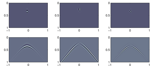
Figure 2: Wavelets and vaguelettes.

Figure 2 shows a vertical, a horizontal and a diagonal Daubechies 10 wavelet and the corresponding vaguelettes obtained by application of the operator $\mathbf{A}$.

4 Inversion from noisy data

In what follows, we assume $(\psi_{\lambda})_{\lambda\in\Lambda}$ to be an orthonormal compactly supported wavelet basis of $L^{2}(\mathbb{R}^{d})$. Further, by $(u_{\lambda})_{\lambda\in\Lambda}$ we denote the corresponding vaguelette basis of $\mathrm{ran}\left(\mathbf{A}\right)\subseteq L^{2}(\mathbb{R}^{d})$ that satisfies $\mathbf{A}\psi_{\lambda}=u_{\lambda}$.

If exact data are available, then the WVD decomposition (15) provides an exact reconstruction formula for the unknown $f$. However, in practical applications the data $\mathbf{A}f$ (or $\mathbf{U}h$) are only known up to some errors (e.g. noise). We therefore assume that we are given erroneous (noisy) data

$$g=\mathbf{A}f+z\,,$$ (17)

where $z$ is the error term and $f$ the exact unknown. We consider both the deterministic and the stochastic case, in which different models for $z$ are assumed:

• In the deterministic case, we assume that a bound $\lVert z\rVert_{L^{2}}\leq\delta$ is available.

• In the stochastic case, we assume that $z=\delta Z$, where $Z$ is a white noise process.

In the deterministic situation the constant $\delta>0$ is referred to as the noise level; in the stochastic case it is the noise standard deviation. The goal in both situations is to estimate the unknown $f\in L^{2}(\mathbb{R}^{d})$ from data in (17).

4.1 Vaguelette-thresholding estimator

In Section 3 we have shown that the reproducing formula $f=\mathbf{A}^{*}\mathbf{A}f=\sum_{\lambda\in\Lambda}\left\langle\mathbf{A}f,u_{\lambda}\right\rangle_{L^{2}}\psi_{\lambda}$ holds in the case of exact data. If the data is corrupted by noise, i.e., $g=\mathbf{A}f+z$, the inner products $\left\langle\mathbf{A}f,u_{\lambda}\right\rangle_{L^{2}}$ cannot be computed exactly. Instead, they are estimated by first evaluating $\left\langle g,u_{\lambda}\right\rangle_{L^{2}}$ and then applying the soft-thresholding operation

$$\mathbf{s}_{w}\colon\mathbb{R}\to\mathbb{R}\colon y\mapsto\begin{cases}y+w&\text{ if }y<-w\\ 0&\text{ if }y\in[-w,w]\\ y-w&\text{ if }y>w\\ \end{cases}$$ (18)

with appropriate thresholds $w=w_{j}$.

Definition 7 (WVD soft thresholding estimator).

For any nonnegative sequence $w=(w_{j})_{j}$, the WVD soft thresholding-estimator for the solution of (17) is defined by

$$\mathbf{S}_{w}\colon L^{2}(\mathbb{R}^{d})\to L^{2}(\mathbb{R}^{d})\colon g\mapsto\sum_{\lambda}\mathbf{s}_{w_{j}}(\left\langle g,u_{\lambda}\right\rangle_{L^{2}})\,\psi_{\lambda}\,,$$ (19)

with the nonlinear soft-thresholding function $\mathbf{s}_{\mu}$ defined in (18).

In the deterministic case we assume that the error term $z$ is known to satisfy $\lVert z\rVert\leq\delta$. In this case, due the isometry property of the operator $\mathbf{A}$, one obtains a stable reconstruction by applying the adjoint $\mathbf{A}^{\ast}$,

$$\forall f\in L^{2}(\mathbb{R}^{d})\colon\quad\sup_{\lVert z\rVert\leq\delta}\lVert f-\mathbf{A}^{\ast}(\mathbf{A}f+z)\rVert=\delta\,.$$ (20)

As the adjoint operator satisfies $\mathbf{A}^{\ast}=\mathbf{S}_{0}$, i.e., $\mathbf{A}^{*}$ corresponds to the WVD-thresholding estimator with $w=0$, it follows that also the class of WVD-thresholding estimators yields the optimal error estimate. Without additional knowledge about the noise there is no need to apply the WVD soft-thresholding estimator with $w\neq 0$, even if the function $f$ is known to belong to some smoothness class, such as a Sobolev or Besov ball. However, if a portion of the noise energy is known to correspond to high frequency components, then using non-zero thresholds may significantly outperform $\mathbf{A}^{\ast}$ given that $f$ belongs to some smoothness class. For example, this happens in the case of stochastic white noise, where the energy-spectrum is uniformly distributed.

4.2 Optimality of vaguelette-thresholding

Suppose $z=\delta Z$, where $Z$ is a white noise process. In the case of random noise, it is common to measure the performance of an estimator $\mathbf{R}\colon L^{2}(\mathbb{R}^{d})\to L^{2}(\mathbb{R}^{d})$ in terms of the worst-case risk [33, 62, 32, 93] of a subset $\mathcal{M}\subseteq L^{2}(\mathbb{R}^{d})$,

$$\boldsymbol{\Delta}(\mathbf{R},\delta,\mathcal{M})=\sup_{f\in\mathcal{M}}\mathbb{E}\left(\left\lVert f-\mathbf{R}(\mathbf{A}f+\delta Z)\right\rVert_{L^{2}}^{2}\right)\,.$$ (21)

Further define the nonlinear minimax risk, the minimax risk using the WVD estimator (19) and the linear minimax risk, respectively by

$$\boldsymbol{\Delta}_{\rm N}(\delta,\mathcal{M}) \coloneqq\inf_{\mathbf{R}}\sup_{f\in\mathcal{M}}\mathbb{E}\left(\left\lVert f-\mathbf{R}(\mathbf{A}f+\delta Z)\right\rVert_{L^{2}}^{2}\right)\,,$$

$$\boldsymbol{\Delta}_{\rm W}(\delta,\mathcal{M}) \coloneqq\inf_{w\in[0,\infty)^{\mathbb{N}}}\sup_{f\in\mathcal{M}}\mathbb{E}\left(\left\lVert f-\mathbf{S}_{w}(\mathbf{A}f+\delta Z)\right\rVert_{L^{2}}^{2}\right)\,,$$

$$\boldsymbol{\Delta}_{\rm L}(\delta,\mathcal{M}) \coloneqq\inf_{\text{$\mathbf{R}$ linear}}\sup_{f\in\mathcal{M}}\mathbb{E}\left(\left\lVert f-\mathbf{R}(\mathbf{A}f+\delta Z)\right\rVert_{L^{2}}^{2}\right)\,.$$

From the definition it is clear that no reconstruction method $\mathbf{R}\colon L^{2}(\mathbb{R}^{d})\to L^{2}(\mathbb{R}^{d})$ can have worst-case risk $\boldsymbol{\Delta}(\mathbf{R},\delta,\mathcal{M})$ smaller than the non-linear minimax risk $\boldsymbol{\Delta}_{\rm N}(\delta,\mathcal{M})$. We are in particular interested in asymptotic behavior for the case $\delta\to 0$ and $\mathcal{M}$ is a ball in a Besov space.

Theorem 8.

Suppose that $r>d(1/p-1/2)$ and let $\mathcal{M}$ be a ball in the Besov-norm having the form

$$\mathcal{M}=\left\{f\in L^{2}(\mathbb{R}^{d})\mid\left\lVert f\right\rVert_{\mathcal{B}_{p,q}^{r}}<\varrho\right\}\quad\text{ for some $\varrho>0$}\,.$$ (22)

Then, as $\delta\to 0$, the following hold

1. $\boldsymbol{\Delta}_{\rm N}(\delta,\mathcal{M})\asymp\delta^{\frac{2r}{r+d/2}}$,

2. $\boldsymbol{\Delta}_{\rm W}(\delta,\mathcal{M})\leq c_{\rm W}\,\boldsymbol{\Delta}_{\rm N}(\delta,\mathcal{M})$ for some constant $c_{\rm W}>0$,

3. $\boldsymbol{\Delta}_{\rm L}(\delta,\mathcal{M})\asymp\delta^{2\frac{r+d(1/2-1/p_{-})}{r+d(1-1/p_{-})}}$ with $p_{-}\coloneqq\min\left\{2,p\right\}$.

Proof.

Follows from [33, Theorem 4] for the special case $\kappa_{j}=1$. ∎

Theorem 8 implies that, despite its simplicity, the WVD-thresholding estimator is order optimal on any Besov-ball and the rate cannot be improved by any other estimator (up to some constant factors). On the other hand, if $p<2$, then the exponent in the linear minimax rate is strictly smaller than the exponent in the non-linear minimax rate, $\tfrac{r+d(1/2-1/p_{-})}{r+d(1-1/p_{-})}<\tfrac{r}{r+d/2}$. Therefore, no linear estimator can give the optimal convergence order. In particular, this implies that the WVD-thresholding estimator outperforms filter based regularization methods including the truncated SVD or quadratic Tikhonov regularization.

4.3 Variational characterizations and extensions

The WVD-based soft thresholding estimation can be characterized via various variational minimization schemes that, as we shall discuss later, in turn offer several extension of the WVD-estimators.

Theorem 9 (Variational characterizations of vaguelette thresholding).

Let $(w_{j})_{j}$ be a sequence of thresholds and let $g,\hat{f}\in L^{2}(\mathbb{R}^{d})$. Then the following assertions are equivalent:

1. $\hat{f}=\mathbf{S}_{w}(g)$;

2. $\hat{f}=\operatorname*{\mathrm{arg\>min}}\left\{\tfrac{1}{2}\left\lVert\mathbf{A}f-g\right\rVert^{2}+\sum_{\lambda\in\Lambda}w_{j}\left\lvert\left\langle\psi_{\lambda},f\right\rangle\right\rvert\mid f\in L^{2}(\mathbb{R}^{d})\right\}$;

3. $\hat{f}$ is the unique solution of the constraint optimization problem

   $$\left\{\begin{aligned} &\min_{f\in L^{2}(\mathbb{R}^{d})}&&\frac{1}{2}\left\lVert f\right\rVert_{L^{2}}^{2}\\ &\text{such that}&&\max_{\lambda\in\Lambda}\frac{\left\lvert\left\langle u_{\lambda},g-\mathbf{A}f\right\rangle\right\rvert}{w_{j}}\leq 1\,.\end{aligned}\right.$$ (23)

Proof.

$\ref{thm:var1}\Leftrightarrow\ref{thm:var2}$: Let $\hat{f}$ denote the minimizer of $\tfrac{1}{2}\left\lVert\mathbf{A}f-g\right\rVert^{2}+\sum_{\lambda\in\Lambda}w_{j}\left\lvert\left\langle\psi_{\lambda},f\right\rangle\right\rvert$. Because $(u_{\lambda})_{\lambda\in\Lambda}$ is an orthonormal basis of $\mathrm{ran}\left(\mathbf{A}\right)$ we have $\lVert\mathbf{A}f-g\rVert^{2}=\lVert\mathcal{P}_{\mathrm{ran}\left(\mathbf{A}\right)^{\bot}}(g)\rVert^{2}+\sum_{\lambda\in\Lambda}\left\lvert\left\langle\mathbf{A}f-g,u_{\lambda}\right\rangle\right\rvert^{2}$. Further, $\sum_{\lambda\in\Lambda}w_{j}\left\lvert\left\langle\psi_{\lambda},f\right\rangle\right\rvert=\sum_{\lambda\in\Lambda}w_{j}\left\lvert\left\langle u_{\lambda},\mathbf{A}f\right\rangle\right\rvert$, which shows that $\hat{f}$ is the unique minimizer of

$$\sum_{\lambda\in\Lambda}\tfrac{1}{2}\left\lvert\left\langle\mathbf{A}f-g,u_{\lambda}\right\rangle\right\rvert^{2}+w_{j}\left\lvert\left\langle u_{\lambda},\mathbf{A}f\right\rangle\right\rvert\,.$$

The latter functional is minimized by minimizing every summand

$$\Phi(\left\langle\mathbf{A}f,u_{\lambda}\right\rangle;w_{j})=\tfrac{1}{2}\left\lvert\left\langle\mathbf{A}f,u_{\lambda}\right\rangle-\left\langle g,u_{\lambda}\right\rangle\right\rvert^{2}+w_{j}\left\lvert\left\langle u_{\lambda},\mathbf{A}f\right\rangle\right\rvert$$

independently in the first argument. The minimizer is given by one-dimensional soft thresholding which gives $\langle\hat{f},\psi_{\lambda}\rangle=\langle\mathbf{A}\hat{f},u_{\lambda}\rangle=\mathbf{s}_{w_{k}}(\langle g,u_{\lambda}\rangle)$ and therefore $\hat{f}=\mathbf{S}_{w}(g)$.

$\ref{thm:var1}\Leftrightarrow\ref{thm:var3}$: Let $\hat{f}$ denote the solution of (23). Using that $(\psi_{\lambda})_{\lambda\in\Lambda}$ is an orthogonal basis and $\psi_{\lambda}=\mathbf{A}^{*}u_{\lambda}$, shows that $\hat{f}$ can be equivalently characterized as the minimizer of

$$\left\{\begin{aligned} &\min_{f\in L^{2}(\mathbb{R}^{d})}&&\frac{1}{2}\sum_{\lambda\in\Lambda}\left\lvert\left\langle\mathbf{A}f,u_{\lambda}\right\rangle\right\rvert^{2}\\ &\text{such that}&&\max_{\lambda\in\Lambda}\frac{\left\lvert\left\langle u_{\lambda},g-\mathbf{A}f\right\rangle\right\rvert}{w_{j}}\leq 1\,.\end{aligned}\right.$$ (24)

The minimization problem (24) can again be solved separately for every component $\left\langle\mathbf{A}f,u_{\lambda}\right\rangle$ which is again given by the one-dimensional soft thresholding $\langle\mathbf{A}\hat{f},u_{\lambda}\rangle=\mathbf{s}_{w_{j}}(\langle g,u_{\lambda}\rangle)$. As above this implies $\hat{f}=\mathbf{S}_{w}(g)$. ∎

The variational characterizations of Theorem 9 have several important implications. First, they provide an explicit minimizer for the $\ell^{1}$-Tikhonov functional

$$\boldsymbol{\Phi}_{g,w}(f)\coloneqq\frac{1}{2}\left\lVert\mathbf{A}f-g\right\rVert^{2}+\sum_{\lambda\in\Lambda}w_{j}\left\lvert\left\langle\psi_{\lambda},f\right\rangle\right\rvert,$$

which in general has to be minimized by an iterative algorithm, such as the iterative soft thresholding algorithm and its variants [26, 27, 30, 8]. For the analysis of $\ell^{1}$-Tikhonov regularization for inverse problems see [30, 48, 49, 69]. Another important consequence is that the WVD-soft thresholding estimator can be generalized in various directions. In particular, one can get a generalization of (23) by replacing the $L^{2}$-norm in (23) by an appropriate regularization functional $\mathcal{J}$ (for example, $\mathcal{J}$ can be chosen as the total variation norm, see Section 5.3). That is, instead of solving the problem (23), one aims at solving the problem

$$\left\{\begin{aligned} &\min_{f\in L^{2}(\mathbb{R}^{d})}&&\mathcal{J}(f)\\ &\text{such that}&&\max_{\lambda\in\Lambda}\frac{\left\lvert\left\langle u_{\lambda},g-\mathbf{A}f\right\rangle\right\rvert}{w_{j}}\leq 1\,,\end{aligned}\right.$$ (25)

This generalization constitutes a hybrid version that combines the WVD estimator with more general regularization functionals $\mathcal{J}$. Such hybrid approaches have been introduced independently in [18, 34, 70, 89] (see also [21, 24]). It is also related to the Dantzig and multiscale estimators of [19, 41, 43, 50, 56, 74].

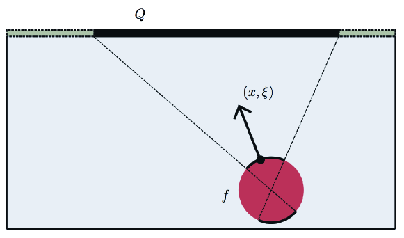
Figure 3: Limited view problem. If data is are collected with finite aperture $Q$, not all features of $f$ can be stably recovered. Only singularities $(x,\xi)$ can be reconstructed for which $x+\mathbb{R}\xi$ intersects $Q$.

5 Numerical implementation

In this section, we provide algorithms for the calculation of the vaguelette transform and the corresponding WVD estimator. Moreover, we consider a hybrid version of the WVD estimator that combines wavelets and TV regularization and discuss its implementation. We also present some numerical examples. Throughout the following $(\psi_{\lambda})_{\lambda\in\Lambda}$ denotes an orthonormal wavelet basis of $L^{2}(\mathbb{R}^{d})$ and $(u_{\lambda})_{\lambda\in\Lambda}$ is the corresponding orthogonal vaguelette basis of $\mathrm{ran}\left(\mathbf{A}\right)\subseteq L^{2}(\mathbb{R}^{d})$ defined by $u_{\lambda}\coloneqq\mathbf{A}\psi_{\lambda}$ (see Section 3).

5.1 Practical aspects

The considered noisy data model (17) assumes that the data can be collected on the whole hyperplane $\partial\mathbb{H}_{+}$. However, this is not feasible in practice since the data can be collected only on a finite subset. In this subsection we discuss the effects of partial (or limited view) data and discretization.

First, we address the limited data issue. In the considered imaging setup, the data is collected on a subset $Q\times[0,T]$ where $Q\subseteq\mathbb{R}^{d-1}$ is the finite measurement aperture (see Figure 3) and $T\in(0,\infty)$ the maximal measurement time. Such partial or limited view data can be modeled by

$$g(x,t)=\left(\chi_{Q\times[0,T]}\,\mathbf{A}f\right)(x,t)\,,$$ (26)

where $\chi_{Q\times[0,T]}$ denotes the characteristic function of $Q\times[0,T]$. Using partial data $g$, only certain features of $h$ can be reconstructed in a stable way, see [6, 45] and Figure 3. Consequently, the practical problem of reconstructing $h$ from partial data, is a limited data problem and therefore severely ill-posed. It is therefore common to incorporate a-priori information into the reconstruction and so to regularize the reconstruction. In this work, we are doing it in two ways: First, we incorporate wavelet sparsity assumptions. This is what the WVD estimator does, which is implemented by evaluating $f^{\dagger}=\sum_{\lambda\in\Lambda}\left\langle g,u_{\lambda}\right\rangle_{L^{2}}\psi_{\lambda}$. The partial reconstruction $f^{\dagger}$ is a “good” approximate reconstruction for $f$, since it recovers all visible boundaries of $f$ correctly and can be evaluated stably. Second, we combine wavelet sparsity with TV regularization by using the using the hybrid estimator (25) to impose even more regularization.

Another practical restriction is that only a finite number of samples of the pressure can be measured. Assuming equidistant sampling and limited view data $g$ as in (26) with $Q=[0,T]^{d-1}$, the actual sampled data are given by

$${\tt g}[n,m]\coloneqq g(n\Delta_{N},m\Delta_{M})+z[n,m]\,,\quad(n,m)\in\left\{1,\dots,N\right\}^{d-1}\times\left\{1,\dots,m\right\}\,.$$ (27)

Here $N$ and $M$ are natural numbers, $\Delta_{N}:=X/N$ and $\Delta_{M}:=T/M$ are the sampling step sizes and $z[n,m]$ decribes the noise in the data. Using Shannon sampling theory it ca be shown that (27) is correctly sampled for $\Delta_{N}=\Delta_{M}\leq\pi/\Omega$, where $\Omega$ is the essential bandwidth of $f$; see [59]. The precise analysis of discretization effects on the considered vaguelette estimators is beyond the scope of this paper.

5.2 Implementation of the vaguelette transform

Analogously to the wavelet transform, we can define the vaguelette transform of $g\in L^{2}(\mathbb{R}^{d})$ corresponding to the operator $\mathbf{A}$ by $\mathcal{V}g\coloneqq\left(\left\langle u_{\lambda},g\right\rangle_{L^{2}}\right)_{\lambda\in\Lambda}$. From the representation $u_{\lambda}=\mathbf{A}\psi_{\lambda}$ and the definition of vaguelette transform we have

$$\forall g\in L^{2}(\mathbb{R}^{d})\;\forall\lambda\in\Lambda\colon\quad(\mathcal{V}g)(\lambda)=\left\langle\mathbf{A}\psi_{\lambda},g\right\rangle_{L^{2}}=\left\langle\psi_{\lambda},\mathbf{A}^{\ast}g\right\rangle_{L^{2}}\,.$$ (28)

Hence, the vaguelette transform can be computed by first applying the adjoint $\mathbf{A}^{*}$ to the data $g$ and then calculating the wavelet transform of $\mathbf{A}^{*}g$.

Algorithm 1 Discrete vaguelette transform

1:Compute $\operatorname{\tt B}{\tt g}\in\mathbb{R}^{N^{d-1}\times M}$ with $\operatorname{\tt B}{\tt g}[n,m]\simeq\mathbf{A}^{*}g(n\Delta_{N},\Delta_{M})$

2:Compute the discrete wavelet transform $\operatorname{\tt W}\operatorname{\tt B}{\tt g}$

Assuming discrete data ${\tt g}\in\mathbb{R}^{N^{d-1}\times M}$ of the form ${\tt g}[n,m]=g(n\Delta_{N},m\Delta_{M})$, the discrete vaguelette transform can efficiently be computed by Algorithm 1. Both the steps in this algorithm are well known and numerically efficient. For the first step we use a numerical approximation of $\mathbf{A}^{*}$ by numerically implementing (11) with a filtered backprojection (FBP) algorithm (see [15, 16]). For evaluating the second step we use the implementation of the fast discrete wavelet transform provided by the Matlab function wavedec2.

5.3 Implementation of the reconstruction algorithms

For the numerical experiments, that will be presented in the next section, we implement the WVD soft-thresholding estimator defined by (19) as well as a hybrid vaguelette-TV approach defined by (25) with $\mathcal{J}(f)=\left\lVert f\right\rVert_{\rm TV}$ being the TV norm of $f$. In both cases we choose $q$ as a half of the so called universal threshold $\sigma\sqrt{2\log(N^{d}M)}$ that can be derived from extreme value theory [32, 55].

The implementation of the WVD soft-thresholding estimator is summarized in Algorithm 2. It is based on the discrete vaguelette transform that was presented in Algorithm 1.

Algorithm 2 WVD soft-thresholding estimator.

1:Compute vaguelette coefficients ${\tt c}=\operatorname{\tt V}{\tt g}$ by applying Algorithm 1

2:Apply soft thresholding to ${\tt c}$ using threshold $q$

3:Apply the inverse wavelet transform

Given discrete data, the hybrid vaguelette-TV approach can be written in the form

$$\min_{{\tt f}}\left\lVert{\tt f}\right\rVert_{\rm TV}\quad\text{ such that }\left\lVert\operatorname{\tt W}(\operatorname{\tt B}{\tt g}-{\tt f})\right\rVert_{\infty}\leq q\,,$$ (29)

where $\operatorname{\tt B}$ denotes the discrete FBP operator. One recognizes that (29) can be implemented by applying a hybrid wavelet-TV denoising algorithm to $\operatorname{\tt B}{\tt g}$. Following [42], we rewrite the optimization problem (29) in the form

$$\min_{{\tt f},{\tt v}}\left\lVert{\tt f}\right\rVert_{\rm TV}+i_{\{\left\lVert\operatorname{\tt W}{\tt v}\right\rVert_{\infty}\leq w\}}\quad\text{ such that }{\tt f}+{\tt v}=\operatorname{\tt B}{\tt g}\,,$$ (30)

and introduce the associated augmented Lagrangian operator

$$\mathcal{L}_{c}\left({\tt f},{\tt v},\mu\right)\coloneqq\left\lVert{\tt f}\right\rVert_{\rm TV}+i_{\{\left\lVert\operatorname{\tt W}{\tt v}\right\rVert_{\infty}\leq w\}}+\left\langle\mu,{\tt f}+{\tt v}-\operatorname{\tt B}{\tt g}\right\rangle+\frac{1}{2c}\left\lVert{\tt f}+{\tt v}-\operatorname{\tt B}{\tt g}\right\rVert_{2}^{2}.$$

Then, (30) can be solved by the alternating direction method of multipliers (ADMM), introduced in [46, 47], which alternatingly performs minimization steps with respect to ${\tt f}$ and ${\tt v}$ and maximization steps with respect to $\mu$. The resulting ADMM algorithm for solving (29) is summarized in Algorithm 3.

Algorithm 3 Hybrid vaguelette-TV approach

1:${\tt f}_{0}={\tt v}_{0}=\mu_{0}=0$

2:for $k=0,1,\dots,N_{\rm iter}$ do

3:     ${\tt f}_{k+1}\in\operatorname*{\mathrm{arg\>min}}{\frac{1}{2}\left\lVert{\tt f}-\left(\operatorname{\tt B}{\tt g}-{\tt v}_{k}-c\mu_{k}\right)\right\rVert_{2}^{2}+c\left\lVert{\tt f}\right\rVert_{\rm TV}}$

4:     ${\tt v}_{k+1}=q\left(\operatorname{\tt B}{\tt g}-{\tt f}_{k+1}-c\mu_{k}\right)/\max\left\{q,\lVert\operatorname{\tt B}{\tt g}-{\tt f}_{k+1}-c\mu_{k}\rVert_{2}\right\}$

5:     $\mu_{k+1}\coloneqq\mu_{k}+c^{-1}\left({\tt f}_{k+1}+{\tt v}_{k+1}-\operatorname{\tt B}{\tt g}\right)$

6:end for

For performing the ${\tt f}$-update in Algorithm 3 we have to solve the unconstraint total variation minimization problem $\frac{1}{2}\left\lVert{\tt f}-\left(\operatorname{\tt B}{\tt g}-{\tt v}_{k}-c\mu_{k}\right)\right\rVert_{2}^{2}+c\left\lVert{\tt f}\right\rVert_{\rm TV}$. For this purpose we use Chambolle’s dual projection algorithm [20].

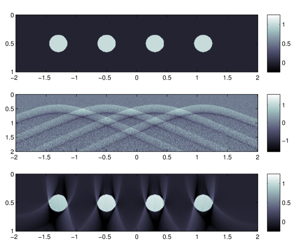
Figure 4: Phantom, data and reconstruction from (noise free) partial data. One notices the typical limited view artifacts in the form of smearing out of almost vertical boundaries.

5.4 Numerical examples

In this section we present a numerical example testing the vaguelette soft-thresholding and the hybrid approach. For that purpose we consider a simple phantom that consists of the superposition of three uniformly absorbing spheres as illustrated in the top image in Figure 4. The data ${\tt g}=\operatorname{\tt A}{\tt f}$ are computed numerically using an implementation according to (10). To simulate data errors, we added i.i.d Gaussian noise with standard deviation $\sigma=0.25$. The relative $\ell^{2}$-error in the noisy data ${\tt g}^{\delta}$ is $\left\lVert{\tt g}^{\delta}-{\tt g}\right\rVert_{2}/\left\lVert{\tt g}\right\rVert_{2}=1.05$.

Figure 5: Reconstructions from noisy data.

Figure 6: Differences between reconstructions from noisy data and the original phantom.

Results of our reconstruction from noisy data are shown Figure 5. The top image shows the non-regularized reconstruction ${\tt f}_{\rm FBP}^{\delta}=\operatorname{\tt A}{\tt g}^{\delta}$, the middle image the vaguelette-thresholding reconstruction ${\tt f}_{\rm WVD}^{\delta}$ and the bottom image the reconstruction with the hybrid vaguelette-TV method ${\tt f}_{\rm hybrid}^{\delta}$. Figure 6 shows corresponding difference images between the reconstructions and the true phantom ${\tt f}$. One clearly observes that the vaguelette estimators significantly reduce the error in the reconstruction. This can be quantified by the relative $\ell^{2}$-errors, which are equal to $\lVert{\tt f}_{\rm FBP}^{\delta}-{\tt f}\rVert_{2}/\lVert{\tt f}\rVert_{2}=0.66$ for the unregularized reconstruction, $\lVert{\tt f}_{\rm WVD}^{\delta}-{\tt f}\rVert_{2}/\lVert{\tt f}\rVert_{2}=0.38$ for the vaguelette thresholding estimator $\lVert{\tt f}_{\rm hybrid}^{\delta}-{\tt f}\rVert_{2}/\lVert{\tt f}\rVert_{2}=0.42$ for the hybrid estimator. The relative $\ell^{2}$-error for the hybrid reconstruction is slightly larger than for the vaguelette-thresholding estimator. This is reasonable since the vaguelette-thresholding estimator minimizes the $\ell^{2}$-norm (see (23)) among all potential reconstructions ${\tt f}$ that are compatible with the data, whereas the hybrid estimator minimizes the total variation. However, in some more appropriate error measure the hybrid reconstruction may outperform the thresholding estimator. Further note that all reconstruction methods contain some limited data artifacts, which cannot removed completely by wavelet methods [6, 45, 59, 75, 90].

6 Conclusion

In this paper we developed a regularization framework using wavelet sparsity in photoacoustic tomography. For that purpose we derived wavelet-vaguelette (WVD) decompositions (see Theorem 6) and an easy but efficient implementation of the corresponding vaguelette transform (see Algorithm 1). Using the WVD we derived an explicit formula for minimizing the sparse Tikhonov functional that can be implemented without any iterative reconstruction procedure (see Algorithm 2). The considered regularization approach has been shown to provide optimal error estimates in the deterministic as well as in the stochastic setting (see Theorem 8). In order to account for wavelet artifacts we also developed hybride regularization methods combining wavelet sparsity with total variation (see Algorithm 3). Numerical results demonstrate the feasibility and efficiency of our reconstruction approaches. Future work will be done to extend our approach to more general measurements geometries in PAT and also to different Radon type inverse problems.

Appendix A Orthogonal wavelets

We recall some basic facts about orthogonal wavelets as we need them for our purpose (in particular in Section 3). For task of function estimation, wavelets are known to sparsely represent many signals and, hence, they can be used to effectively encode prior information. Another useful property of wavelets consists in the ability to characterize several classical smoothness measures (eg. Sobolev and Besov norms) in terms of the decay properties of wavelet coefficients. We will also use that property in Section 4. For a detailed introduction to wavelets we refer to [23, 29, 71].

A.1 One-dimensional wavelets

We first briefly recall the basic definitions and notations of orthonormal wavelet bases (wavelet ONB) in one spatial dimension, which will be then extended to higher dimensions.

The construction of a wavelet ONB is based on the concept of a multiresolution analysis (MSA), which is given by a sequence subspaces $(V_{j})_{j\in\mathbb{Z}}$ in $L^{2}\left(\mathbb{R}\right)$ that satisfy the following requirements (see [23, 29, 71]):

• For all $j\in\mathbb{Z}$ it holds that $V_{j}\subseteq V_{j+1}$.

• The union $\bigcup_{j\in\mathbb{N}}\mathrm{V}_{j}$ is dense in $L^{2}\left(\mathbb{R}\right)$.

• $\bigcap_{j\in\mathbb{Z}}\mathrm{V}_{j}=\left\{0\right\}$ .

• For every $j\in\mathbb{N}$, we have $f\in\mathrm{V}_{j}\iff f(\tfrac{\,\cdot\,}{2})\in\mathrm{V}_{j+1}$.

• There is a function $\varphi\in L^{2}\left(\mathbb{R}\right)$ such that the translates $(\varphi(\cdot-k))_{k\in\mathbb{Z}}$ constitute an ONB of the scaling space $V_{0}$.

The function $\varphi$ is called scaling function and the spaces $V_{j}$ are called scaling (or approximation) spaces at scale j. To each scaling space $V_{j}$, one can associate a wavelet (or detail) space $W_{j}$, that are defined to be the orthogonal complements of $V_{j}$ in $V_{j+1}$, i.e., $V_{j+1}=V_{j}\oplus W_{j}$. Because of the above properties it holds that, for each $j\in\mathbb{Z}$ and $t\in\mathbb{R}$, the functions

$$t\mapsto\varphi_{j,k}\left(t\right)\coloneqq 2^{j/2}\varphi\left(2^{j}t-k\right)$$

constitute an ONB for the scaling space $V_{j}$. One can also show that from the existence of the scaling function it follows that there exists a so-called generating wavelet (or mother wavelet) $\psi\in L^{2}\left(\mathbb{R}\right)$ such that, for each $j\in\mathbb{Z}$ and $t\in\mathbb{R}$, the functions

$$\psi_{j,k}\left(t\right)\coloneqq 2^{j/2}\varphi\left(2^{j}t-k\right)$$

constitute an ONB for the spaces $W_{j}$. Hence, we have that, for every $j\in\mathbb{Z}$, the following mappings are bijections:

$$\mathrm{V}_{j}\to\ell^{2}(\mathbb{Z}) \colon f\mapsto\left(\left\langle\varphi_{j,k},f\right\rangle\mid k\in\mathbb{Z}\right)\,,$$

$$\mathrm{W}_{j}\to\ell^{2}(\mathbb{Z}) \colon f\mapsto\left(\left\langle\psi_{j,k},f\right\rangle\mid k\in\mathbb{Z}\right)\,.$$

The above constructions provide the following decompositions of the signal space $L^{2}\left(\mathbb{R}\right)$ into the sum of the scaling spaces $\mathrm{V}_{j}$ and the wavelet spaces $\mathrm{W}_{j}$, or into a sum of only wavelet spaces:

$$L^{2}\left(\mathbb{R}\right)=V_{0}\oplus\bigoplus_{j\geq 0}W_{j}=\bigoplus_{j\in\mathbb{Z}}W_{j}.$$

From these decomposition we immediately get the following decompositions of signals $f\in L^{2}\left(\mathbb{R}\right)$:

$$f =\sum_{k\in\mathbb{Z}}\langle f,\varphi_{0,k}\rangle\varphi_{0,k}+\sum_{j\geq 0}\sum_{k\in\mathbb{Z}}\langle f,\psi_{j,k}\rangle\psi_{j,k}$$

$$=\sum_{j\in\mathbb{Z}}\sum_{k\in\mathbb{Z}}\langle f,\psi_{j,k}\rangle\psi_{j,k}.$$

The coefficients of the above decomposition are called the wavelet and scaling coefficients of $f$, respectively, and the corresponding mapping that maps $f$ to those coefficients is called the wavelet transform of $f$. A detailed construction of orthogonal (and biorthogonal) wavelet systems together with many interesting details may be found, for example, in [23, 29, 71].

A.2 Wavelets in higher dimension

Wavelet bases in higher dimensions can be defined by taking tensor products of the one-dimensional wavelet and scaling functions. As a concrete example consider $L^{2}(\mathbb{R}^{2})\cong L^{2}(\mathbb{R})\otimes L^{2}(\mathbb{R})$ and let $\psi,\varphi\colon\mathbb{R}\to\mathbb{R}$ be the generating wavelet and scaling functions, respectively. Then, an orthogonal wavelet basis of $L^{2}(\mathbb{R}^{2})$ is defined by translates and scaled versions of the (tensor product) functions

$$\psi^{(1)}\colon (x,y)\in\mathbb{R}^{2}\mapsto\psi(x)\varphi(y)$$

$$\psi^{(2)}\colon (x,y)\in\mathbb{R}^{2}\mapsto\varphi(x)\psi(y)$$

$$\psi^{(3)}\colon (x,y)\in\mathbb{R}^{2}\mapsto\psi(x)\psi(y)\,.$$

The corresponding scaling functions at scale $j\in\mathbb{Z}$ of two variables are defined as translated and scaled versions of

$$\varphi^{(0)}(x,y)\coloneqq\varphi(x)\varphi(y).$$

Analogously to the above construction in two dimensions, one can define a wavelet ONB in $\mathbb{R}^{d}$ by a tensor product construction. In this case we get $2^{d}-1$ different generating wavelets $\psi^{(\varepsilon)}$ and one generating scaling function $\varphi^{(0)}$. Therefore, a wavelet ONB in $\mathbb{R}^{d}$ is system $(\psi_{\lambda})_{\lambda\in\Lambda}$ in $L^{2}(\mathbb{R}^{d})$, where the index $\lambda=(j,k,\varepsilon)$ consists of three parameters, the scale index $j\in\mathbb{Z}$, the location index $k\in\mathbb{Z}^{d}$, and the orientation index $\varepsilon\in\left\{1,2,\dots,2^{d}-1\right\}$. The wavelet basis elements are again defined as dilates and translates of the generating wavelets $\psi^{(\varepsilon)}$:

$$\psi_{j,k,\varepsilon}(x)=2^{-jd/2}\,\psi^{(\varepsilon)}(2^{j}x-k)\,.$$ (31)

If we also add the index set $\Lambda_{-1}\coloneqq\left\{0\right\}\times\mathbb{Z}^{d}$ and consider the scaling functions defined by

$$\varphi_{0,k}^{\varepsilon}(x)=2^{-jd/2}\varphi^{(0)}(2^{j}x-k),$$

the we get similar decompositions to the one-dimensional case:

$$f =\sum_{k\in\mathbb{Z}^{d}}\langle f,\varphi_{0,k}\rangle\varphi_{0,k}+\sum_{j\geq 0}\sum_{k\in\mathbb{Z}^{d}}\sum_{\varepsilon=1}^{2^{d}-1}\langle f,\psi_{j,k,\varepsilon}\rangle\psi_{j,k,\varepsilon}$$

$$=\sum_{j\in\mathbb{Z}}\sum_{k\in\mathbb{Z}^{d}}\sum_{\varepsilon=1}^{2^{d}-1}\langle f,\psi_{j,k,\varepsilon}\rangle\psi_{j,k,\varepsilon}.$$

For $f\in L^{2}(\mathbb{R}^{d})$ we define the wavelet transform as

$$(\mathcal{W}f)\colon\Lambda\to\mathbb{R}\colon\lambda\mapsto(\mathcal{W}f)(\lambda)\coloneqq\left\langle\psi_{\lambda},f\right\rangle\,.$$ (32)

Then the wavelet transform $\mathcal{W}\colon L^{2}\left(\mathbb{R}^{d}\right)\to\ell^{2}\left(\Lambda\right)\colon f\mapsto\mathcal{W}f$ is an isometric isomorphism with the reproducing property $f=\mathcal{W}^{*}\mathcal{W}f$.

A.3 Besov spaces

Orthonormal wavelet bases can be used to characterize smoothness of functions in terms of the decay properties of wavelet coefficients. In particular, wavelets provide a convenient and a numerically efficient way to characterize Besov spaces and calculate Besov smoothness of functions, see [23]. Skipping the details, we here only mention that the Besov spaces $\mathcal{B}_{p,q}^{s}(\mathbb{R}^{d})$ can be defined by the condition, that the Besov norm

$$\left\lVert f\right\rVert_{\mathcal{B}_{p,q}^{r}}=\sqrt[p]{\sum_{j\in\mathbb{N}}2^{jsq}\,\left\lVert\mathcal{W}f\left(j,\,\cdot\,\right)\right\rVert_{\ell^{p}}^{q}}\qquad\text{ with }\quad s=r+\frac{d}{2}-\frac{d}{p}\,,$$

is well defined and finite. We note that, the given definition of $\left\lVert\,\cdot\,\right\rVert_{\mathcal{B}_{p,q}^{r}}$ is an equivalent norm to the classical definition of Besov norms. The above characterization holds as long as the generating wavelet has $m>r$ vanishing moments and is $m$-times continuously differentiable.

In Section 4, we use the above characterization of Besov norms in terms of wavelet coefficients in order to evaluate the performance of our method for functions that lie in balls of Besov spaces $\mathcal{B}_{p,q}^{s}(\mathbb{R}^{d})$ for some given norm parameters $p$, $q\geq 1$ and smoothness parameter $r\geq 0$.

References

- [1] F. Abramovich and B. W. Silverman. Wavelet decomposition approaches to statistical inverse problems. Biometrika, 85(1):115–129, 1998.
- [2] M. Agranovsky and P. Kuchment. Uniqueness of reconstruction and an inversion procedure for thermoacoustic and photoacoustic tomography with variable sound speed. Inverse Probl., 23(5):2089–2102, 2007.
- [3] M. Agranovsky, P. Kuchment, and L. Kunyansky. On reconstruction formulas and algorithms for the thermoacoustic tomography. In L. V. Wang, editor, Photoacoustic imaging and spectroscopy, chapter 8, pages 89–101. CRC Press, 2009.
- [4] L.-E. Andersson. On the determination of a function from spherical averages. SIAM J. Math. Anal., 19(1):214–232, 1988.
- [5] S. R. Arridge, M. M. Betcke, B. T. Cox, F. Lucka, and B. E. Treeby. On the adjoint operator in photoacoustic tomography. Inverse Probl., 32(11):115012 (19pp), 2016.
- [6] L. L. Barannyk, J. Frikel, and L. V. Nguyen. On artifacts in limited data spherical radon transform: Curved observation surface. Inverse Probl., 32(1), 2015.
- [7] P. Beard. Biomedical photoacoustic imaging. Interface focus, 1(4):602–631, 2011.
- [8] A. Beck and M. Teboulle. A fast iterative shrinkage-thresholding algorithm for linear inverse problems. SIAM J. Imaging Sci., 2(1):183–202, 2009.
- [9] A. Beltukov. Inversion of the spherical mean transform with sources on a hyperplane, 2009. arXiv:0919.1380v1.
- [10] M. M. Betcke, B. T. Cox, N. Huynh, E. Z. Zhang, P. C. Beard, and S. R. Arridge. Acoustic wave field reconstruction from compressed measurements with application in photoacoustic tomography, 2016. arXiv preprint arXiv:1609.02763.
- [11] P. J. Bickel, Y. Ritov, and A. B. Tsybakov. Simultaneous analysis of lasso and dantzig selector. Ann. Statist., pages 1705–1732, 2009.
- [12] K. Bredies and D. Lorenz. Iterated hard shrinkage for minimization problems with sparsity constraints. SIAM J. Sci. Comput., 30(2):657–683, 2008.
- [13] A. L. Buhgeim and V. B. Kardakov. Solution of an inverse problem for an elastic wave equation by the method of spherical means. Sibirsk. Mat. Z., 19(4):749–758, 1978.
- [14] M. Burger, J. Flemming, and B. Hofmann. Convergence rates in -regularization if the sparsity assumption fails. Inverse Probl., 29(2):025013, 16, 2013.
- [15] P. Burgholzer, J. Bauer-Marschallinger, H. Grün, M. Haltmeier, and G. Paltauf. Temporal back-projection algorithms for photoacoustic tomography with integrating line detectors. Inverse Probl., 23(6):S65–S80, 2007.
- [16] P. Burgholzer, G. J. Matt, M. Haltmeier, and G. Paltauf. Exact and approximate imaging methods for photoacoustic tomography using an arbitrary detection surface. Phys. Rev. E, 75(4):046706, 2007.
- [17] E. J. Candès and D. Donoho. Recovering edges in ill-posed inverse problems: Optimality of curvelet frames. Ann. Statist., 30(3):784–842, 2002.
- [18] E. J. Candès and F. Guo. New multiscale transforms, minimum total variation synthesis: applications to edge preserving image reconstruction. Signal Process., 82:1519—1543, 2002.
- [19] E. J. Candès and T. Tao. The Dantzig selector: statistical estimation when is much larger than . Ann. Statist., 35(6):2313–2351, 2007.
- [20] A. Chambolle. An algorithm for total variation minimization and applications. J. Math. Imaging Vision, 20(1–2):89–97, 2004.
- [21] T. F. Chan and H. Zhou. Total variation improved wavelet thresholding in image compression. In EEE International Conference on Image Processing, volume 2, pages 391–394. IEEE, 2000.
- [22] S. S. Chen, D. L. Donoho, and M. A. Saunders. Atomic decomposition by basis pursuit. SIAM Rev., 43(1):129–159, 2001. Reprinted from SIAM J. Sci. Comput. 20 (1998), no. 1, 33–61.
- [23] A. Cohen. Numerical Analysis of Wavelet Methods, volume 32 of Studies in Mathematics and its Applications. North-Holland Publishing Co., Amsterdam, 2003.
- [24] R. R. Coifman and A. Sowa. Combining the calculus of variations and wavelets for image enhancement. Appl. Comput. Harmon. Anal., 9(1):1–18, 2000.
- [25] F. Colonna, G. Easley, K. Guo, and D. Labate. Radon transform inversion using the shearlet representation. Appl. Comput. Harmon. Anal., 29(2):232–250, 2010.
- [26] P. L. Combettes and J.-C. Pesquet. Proximal splitting methods in signal processing. In Fixed-point algorithms for inverse problems in science and engineering, pages 185–212. Springer, 2011.
- [27] P. L. Combettes and V. R. Wajs. Signal recovery by proximal forward-backward splitting. Multiscale Model. Sim., 4(4):1168–1200 (electronic), 2005.
- [28] R. Courant and D. Hilbert. Methods of Mathematical Physics, volume 2. Wiley-Interscience, New York, 1962.
- [29] I. Daubechies. Ten Lectures on Wavelets. SIAM, Philadelphia, PA, 1992.
- [30] I. Daubechies, M. Defrise, and C. De Mol. An iterative thresholding algorithm for linear inverse problems with a sparsity constraint. Comm. Pure Appl. Math., 57(11):1413–1457, 2004.
- [31] X. L. Dean-Ben, A. Buehler, V. Ntziachristos, and D. Razansky. Accurate model-based reconstruction algorithm for three-dimensional optoacoustic tomography. IEEE Trans. Med. Imag., 31(10):1922–1928, 2012.
- [32] D. L. Donoho. De-noising by soft-thresholding. IEEE Trans. Inf. Theory, 41(3):613–627, 1995.
- [33] D. L. Donoho. Nonlinear solution of linear inverse problems by wavelet–vaguelette decomposition. Appl. Comput. Harmon. Anal., 2(2):101–126, April 1995.
- [34] S. Durand and J. Froment. Artifact free signal denoising with wavelets. Proceedings of ICASSP 2001 ( 26th International Conference on Acoustics, Speech, and Signal Processing), 6:3685–3688, 2001.
- [35] L. C. Evans. Partial Differential Equations, volume 19 of Graduate Studies in Mathematics. American Mathematical Society, Providence, RI, 1998.
- [36] J. A. Fawcett. Inversion of -dimensional spherical averages. SIAM J. Appl. Math., 45(2):336–341, 1985.
- [37] M. A. Figueiredo and R. D. Nowak. An em algorithm for wavelet-based image restoration. IEEE Trans. Image Process., 12(8):906–916, 2003.
- [38] D. Finch, M. Haltmeier, and Rakesh. Inversion of spherical means and the wave equation in even dimensions. SIAM J. Appl. Math., 68(2):392–412, 2007.
- [39] D. Finch, S. K. Patch, and Rakesh. Determining a function from its mean values over a family of spheres. SIAM J. Math. Anal., 35(5):1213–1240, 2004.
- [40] J. Flemming and B. Hofmann. A new approach to source conditions in regularization with general residual term. Num. Numer. Funct. Anal. Optim., 31(3):254–284, 2010.
- [41] K. Frick, P. Marnitz, and A. Munk. Shape-constrained regularization by statistical multiresolution for inverse problems: asymptotic analysis. Inverse Probl., 28(6):065006, 2012.
- [42] K. Frick, P. Marnitz, and A. Munk. Statistical multiresolution estimation in imaging: Fundamental concepts and algorithmic approach. Electron. J. Statist., 6:231–268, 2012.
- [43] K. Frick, P. Marnitz, and A. Munk. Statistical multiresolution estimation for variational imaging: With an application in poisson-biophotonics. J. Math. Imaging Vision, 46(3):370–387, 2013.
- [44] J. Frikel. Sparse regularization in limited angle tomography. Appl. Comput. Harmon. Anal., 34(1):117–141, 2013.
- [45] J. Frikel and E. T. Quinto. Artifacts in incomplete data tomography with applications to photoacoustic tomography and sonar. SIAM J. Appl. Math., 75(2):703–725, 2015.
- [46] D. Gabay and B. Mercier. A dual algorithm for the solution of nonlinear variational problems via finite element approximation. Computers & Mathematics with Applications, 2(1):17–40, 1976.
- [47] R. Glowinski and A. Marroco. Sur l’approximation, par elements finis d’ordre un, et la resolution, par penalisation-dualite, d’une classe de problemes de dirichlet non lineares. Revue Franqaise d’Automatique, Informatique et Recherche Opirationelle, 9:41–76, 1975.
- [48] M. Grasmair, M. Haltmeier, and O. Scherzer. Sparse regularization with penalty term. Inverse Probl., 24(5):055020, 13, 2008.
- [49] M. Grasmair, M. Haltmeier, and O. Scherzer. Necessary and sufficient conditions for linear convergence of -regularization. Comm. Pure Appl. Math., 64(2):161–182, 2011.
- [50] M. Grasmair, H. Li, and A. Munk. Variational multiscale nonparametric regression: Smooth functions. arXiv preprint arXiv:1512.01068, 2015.
- [51] M. Haltmeier. Inversion of circular means and the wave equation on convex planar domains. Comput. Math. Appl., 65(7):1025–1036, 2013.
- [52] M. Haltmeier. Stable signal reconstruction via -minimization in redundant, non-tight frames. IEEE Trans. Signal Process., 61(2):420–426, 2013.
- [53] M. Haltmeier. Universal inversion formulas for recovering a function from spherical means. SIAM J. Math. Anal., 46(1):214–232, 2014.
- [54] M. Haltmeier, T. Berer, S. Moon, and P. Burgholzer. Compressed sensing and sparsity in photoacoustic tomography. J. Opt., 18(11):114004, 2016.
- [55] M. Haltmeier and A. Munk. Extreme value analysis of empirical frame coefficients and implications for denoising by soft-thresholding. Appl. Comput. Harmon. Anal., page in press, 2013.
- [56] M. Haltmeier and A. Munk. A variational view on statistical multiscale estimation, 2017. iIn preparation.
- [57] M. Haltmeier and L. V. Nguyen. Iterative methods for photoacoustic tomography with variable sound speed. arXiv:1611.07563, 2016.
- [58] M Haltmeier and S Pereverzyev Jr. The universal back-projection formula for spherical means and the wave equation on certain quadric hypersurfaces. J. Math. Anal. Appl., 429(1):366–382, 2015.
- [59] M. Haltmeier, O. Scherzer, and G. Zangerl. A reconstruction algorithm for photoacoustic imaging based on the nonuniform FFT. IEEE Trans. Med. Imag., 28(11):1727–1735, November 2009.
- [60] Y. Hristova, P. Kuchment, and L. Nguyen. Reconstruction and time reversal in thermoacoustic tomography in acoustically homogeneous and inhomogeneous media. Inverse Probl., 24(5):055006 (25pp), 2008.
- [61] M. Jaeger, S. Schüpbach, A. Gertsch, M. Kitz, and M. Frenz. Fourier reconstruction in optoacoustic imaging using truncated regularized inverse k-space interpolation. Inverse Probl., 23:S51–S63, 2007.
- [62] I. M. Johnstone. Gaussian estimation: Sequence and wavelet models. Draft of a Monograph, Version October 6 2015.
- [63] E. D. Kolaczyk. A wavelet shrinkage approach to tomographic image reconstruction. J. Amer. Statist. Assoc., 91(435):1079–1090, 1996.
- [64] K. P. Kostli, D. Frauchiger, J. J. Niederhauser, G. Paltauf, H. P. Weber, and M. Frenz. Optoacoustic imaging using a three-dimensional reconstruction algorithm. IEEE Sel. Top. Quant. Electr., 7(6):918–923, 2001.
- [65] R.A Kruger, P. Lui, Y.R. Fang, and R.C. Appledorn. Photoacoustic ultrasound (PAUS) – reconstruction tomography. Med. Phys., 22(10):1605–1609, 1995.
- [66] P. Kuchment and L. Kunyansky. Mathematics of photoacoustic and thermoacoustic tomography. In Handbook of Mathematical Methods in Imaging, pages 817–865. Springer, 2011.
- [67] L. A. Kunyansky. Explicit inversion formulae for the spherical mean Radon transform. Inverse Probl., 23(1):373–383, 2007.
- [68] L. A. Kunyansky. A series solution and a fast algorithm for the inversion of the spherical mean Radon transform. Inverse Probl., 23(6):S11–S20, 2007.
- [69] D. Lorenz. Convergence rates and source conditions for Tikhonov regularization with sparsity constraints. J. Inverse Ill-Posed Probl., 16(5):463–478, 2008.
- [70] F. Malgouyres. Minimizing the total variation under a general convex constraint for image restoration. IEEE Trans. Image Process., 11(12):1450–1456, 2002.
- [71] S. Mallat. A wavelet tour of signal processing: The sparse way. Elsevier/Academic Press, Amsterdam, third edition, 2009.
- [72] E. K. Narayanan and Rakesh. Spherical means with centers on a hyperplane in even dimensions. Inverse Probl., 26(3):035014, March 2010.
- [73] F. Natterer. Photo-acoustic inversion in convex domains. Inverse Probl. Imaging, 6(2):315–320, 2012.
- [74] A. S. Nemirovskii. Nonparametric estimation of smooth regression functions. Izv. Akad. Nauk. SSR Teckhn. Kibernet, 3:50–60, 1985.
- [75] L. V. Nguyen. How strong are streak artifacts in limited angle computed tomography? Inverse Probl., 31(5):055003, 2015.
- [76] L. V. Nguyen and L. A. Kunyansky. A dissipative time reversal technique for photoacoustic tomography in a cavity. SIAM J. Imaging Sci., 9(2):748–769, 2016.
- [77] S. J. Norton and M. Linzer. Ultrasonic reflectivity imaging in three dimensions: Exact inverse scattering solutions for plane, cylindrical and spherical apertures. IEEE Trans. Biomed. Eng., 28(2):202–220, 1981.
- [78] M. R. Osborne, B. Presnell, and B. A. Turlach. On the lasso and its dual. Journal of Computational and Graphical statistics, 9(2):319–337, 2000.
- [79] V. P. Palamodov. A uniform reconstruction formula in integral geometry. Inverse Probl., 28(6):065014, 2012.
- [80] G. Paltauf, R. Nuster, M. Haltmeier, and P. Burgholzer. Experimental evaluation of reconstruction algorithms for limited view photoacoustic tomography with line detectors. Inverse Probl., 23(6):S81–S94, 2007.
- [81] G. Paltauf, R. Nuster, M. Haltmeier, and P. Burgholzer. Photoacoustic tomography with integrating area and line detectors. In Photoacoustic imaging and spectroscopy, chapter 20, pages 251–263. CRC Press, 2009.
- [82] G. Paltauf, J. A. Viator, S. A. Prahl, and S. L. Jacques. Iterative reconstruction algorithm for optoacoustic imaging. J. Opt. Soc. Am., 112(4):1536–1544, 2002.
- [83] X. Pan, E. Y. Sidky, and M. Vannier. Why do commercial ct scanners still employ traditional, filtered back-projection for image reconstruction? Inverse Probl., 25(12):123009, 2009.
- [84] J. Poudel, T. P. Matthews, L. Li, M. A. Anastasio, and L. V. Wang. Mitigation of artifacts due to isolated acoustic heterogeneities in photoacoustic computed tomography using a variable data truncation-based reconstruction method. J. Biomed. Opt., 22(4):041018, 2017.
- [85] J. Provost and F. Lesage. The application of compressed sensing for photo-acoustic tomography. IEEE Trans. Med. Imag., 28(4):585–594, 2009.
- [86] R. Ramlau and G. Teschke. A Tikhonov-based projection iteration for nonlinear ill-posed problems with sparsity constraints. Numer. Math., 104(2):177–203, 2006.
- [87] A. Rosenthal, V. Ntziachristos, and D. Razansky. Acoustic inversion in optoacoustic tomography: A review. Curr. Med. Imaging Rev., 9(4):318, 2013.
- [88] O. Scherzer, M. Grasmair, H. Grossauer, M. Haltmeier, and F. Lenzen. Variational methods in imaging, volume 167 of Applied Mathematical Sciences. Springer, New York, 2009.
- [89] J.-L. Starck, D. Donoho, and E. Candès. Very high quality image restoration by combining wavelets and curvelets. Proc. SPIE, 4478:9, 2011.
- [90] P. Stefanov and G. Uhlmann. Is a curved flight path in sar better than a straight one? SIAM J., 73(4):1596–1612, 2013.
- [91] R. Tibshirani. Regression shrinkage and selection via the lasso. J. Roy. Statist. Soc. Ser. B, 58(1):267–288, 1996.
- [92] B. E. Treeby and B. T. Cox. k-wave: Matlab toolbox for the simulation and reconstruction of photoacoustic wave-fields. J. Biomed. Opt., 15:021314, 2010.
- [93] A. B. Tsybakov. Introduction to nonparametric estimation. Springer Series in Statistics. Springer, New York, 2009.
- [94] S. Vaiter, G. Peyré, C. Dossal, and J. Fadili. Robust sparse analysis regularization. IEEE Trans. Inf. Theory, 59(4):2001–2016, 2013.
- [95] K. Wang and M. A. Anastasio. Photoacoustic and thermoacoustic tomography: image formation principles. In Handbook of Mathematical Methods in Imaging, pages 781–815. Springer, 2011.
- [96] K. Wang, R. W. Schoonover, R. Su, A. Oraevsky, and M. A. Anastasio. Discrete imaging models for three-dimensional optoacoustic tomography using radially symmetric expansion functions. IEEE Trans. Med. Imag., 33(5):1180–1193, 2014.
- [97] K. Wang, R. Su, A. A. Oraevsky, and M. A. Anastasio. Investigation of iterative image reconstruction in three-dimensional optoacoustic tomography. Phys. Med. Biol., 57(17):5399, 2012.
- [98] L. V. Wang. Multiscale photoacoustic microscopy and computed tomography. Nature Phot., 3(9):503–509, 2009.
- [99] M. Xu and L. V. Wang. Universal back-projection algorithm for photoacoustic computed tomography. Phys. Rev. E, 71(1):016706, 2005.
- [100] M. Xu and L. V. Wang. Photoacoustic imaging in biomedicine. Rev. Sci. Instr., 77(4):041101 (22pp), 2006.
- [101] Y. Xu, D. Feng, and L. V. Wang. Exact frequency–domain reconstrcution for thermoacosutic tomography — I: Planar geometry. IEEE Trans. Med. Imag., 21(7):823–828, 2002.
- [102] J. Zhang, M. A. Anastasio, P. J. La Rivière, and L. V. Wang. Effects of different imaging models on least-squares image reconstruction accuracy in photoacoustic tomography. IEEE Trans. Med. Imag., 28(11):1781–1790, 2009.
- [103] H. Zou. The adaptive lasso and its oracle properties. J. Amer. Statist. Assoc., 101(476):1418–1429, 2006.