The $\infty$-Fučík spectrum

Abstract.

In this article we study the behavior as $p\nearrow+\infty$ of the Fučik spectrum for $p$-Laplace operator with zero Dirichlet boundary conditions in a bounded domain $\Omega\subset\mathbb{R}^{n}$. We characterize the limit equation, and we provide a description of the limit spectrum. Furthermore, we show some explicit computations of the spectrum for certain configurations of the domain.

1. Introduction

Given a bounded smooth domain $\Omega\subset\mathbb{R}^{n}$, $n\geq 1$, we are interested in studying the asymptotic behavior as $p\to\infty$ of the following non-linear eigenvalue problem

(1.1) $$\left\{\begin{array}[]{ll}-\Delta_{p}u(x)=\alpha_{p}(u^{+})^{p-1}(x)-\beta_{p}(u^{-})^{p-1}(x)&\text{in }\Omega\\ u(x)=0&\text{on }\partial\Omega,\end{array}\right.$$

where $\Delta_{p}u\mathrel{\mathop{:}}=\mathrm{div}(|\nabla u|^{p-2}\nabla u)$ denotes the $p$-Laplace operator and $\alpha_{p}$ and $\beta_{p}$ are two real parameters. As usual, $u^{\pm}=\max\{0,\pm u\}$ mean the positive and negative parts of $u$. Recall that the set

$$\Sigma_{p}\mathrel{\mathop{:}}=\{(\alpha_{p},\beta_{p})\in\mathbb{R}^{2}\colon\,\,\mbox{there exists a nontrivial solution }u\mbox{ of }\eqref{ecu}\}$$

is currently known as the Fučík spectrum in honor to the Czech mathematician Svatopluk Fučík, who in the late ’70s, studied this kind of equations in one space dimension with periodic boundary conditions and their relationship with jumping nonlinearities. More precisely, in [16] it was proved that $\Sigma_{2}$ for $\Omega=(a,b)\subset\mathbb{R}$ consists in two trivial lines and a family of hyperbolic-like curves passing thought the pairs $(\lambda,\lambda)$, being $\lambda$ an eigenvalue of the (zero) Dirichlet Laplacian in the interval $(a,b)$. Also, explicit formulas for such curves were found. When regarding the one-dimensional case for $p\neq 2$, the structure of the spectrum is similar, see for instance [14]. Throughout the last decades several works have been devoted to studying $\Sigma_{p}$ in $\mathbb{R}^{n}$ (for $n\geq 1$). The bibliography on this subject is vast. For the linear case, $p=2$, we refer to the reader the papers [10, 11, 12, 13, 17, 24, 30]. When $p\neq 2$ we address, for instance, to references [8, 9, 26, 27, 28].

Observe that problem (1.1) is closely related with the eigenvalue problem of the (zero) Dirichlet $p$-Laplacian, since, when both parameters $\alpha_{p}$ and $\beta_{p}$ are considered to be the same, (1.1) becomes

(1.2) $$\left\{\begin{array}[]{ll}-\Delta_{p}u(x)=\lambda|u(x)|^{p-2}u(x)&\text{in }\Omega\\ u(x)=0&\text{on }\partial\Omega\end{array}\right.$$

and it follows that the pair $(\lambda_{k,p},\lambda_{k,p})$ belongs to $\Sigma_{p}$ for each $k\in\mathbb{N}$, where $\lambda_{k,p}$ denotes the $k$-th (variational) eigenvalue of (1.2). It is also straightforward to see that the trivial lines $\{\lambda_{1,p}\}\times\mathbb{R}$ and $\mathbb{R}\times\{\lambda_{1,p}\}$ belong to $\Sigma_{p}$. The following facts are well-known in the the literature, see [10, 11, 12, 13, 17, 24] and [8, 9, 26]: the trivial lines are isolated in the spectrum and curves in $\Sigma_{p}$ emanating from each pair $(\lambda_{k,p},\lambda_{k,p})$ exist locally. Moreover, it is proved that the spectrum contains a continuous non-trivial first curve passing though $(\lambda_{2,p},\lambda_{2,p})$, which is, in fact asymptotic to the trivial lines, and it admits a variational characterization.

Let us recall some important properties on the spectrum of the $p$-Laplacian. For problem (1.2) there exists a sequence of eigenvalues tending to infinity (note that, in general, it is not known if such a sequence constitutes the whole spectrum), that is, ($\lambda_{k,p})_{k\geq 1}$ such that there are nontrivial solutions to the problem (1.2), see [18]. It is also known (cf. [1]) that the first eigenvalue to (1.2) is isolated, simple and can be variationally characterized as

(Eigenv.) $$\lambda_{1,p}(\Omega)=\inf_{u\in W^{1,p}_{0}(\Omega)\setminus\{0\}}\frac{\|\nabla u\|^{p}_{L^{p}(\Omega)}}{\|u\|^{p}_{L^{p}(\Omega)}}.$$

In the last three decades there was an increasing number of works concerning the study of limit for $p$-Laplacian type problems as $p\to+\infty$. In this direction, one of pioneering works is [3] where it was studied the limit of torsional creep type problems for the $p$-Laplacian, namely

$$-\Delta_{p}u_{p}(x)=1\quad\text{in}\quad\Omega,$$

obtaining as “limit equation” $|\nabla u|=1\quad\text{in}\quad\Omega$ (the well-known Eikonal equation) in the viscosity sense. Moreover, $u(x)=\mathrm{dist}(x,\partial\Omega)$ is the corresponding limiting solution (we also recall that more general problems are studied there). On the other hand, regarding the so-called $\infty$-eigenvalue problem, the main reference is [22], where the authors proved that such a quantity is obtained as a limit of the first eigenvalue (Eigenv.) in the following way

$$\lambda_{1,\infty}(\Omega)=\lim_{p\to\infty}\lambda_{1,p}^{1/p}(\Omega).$$

An interesting piece of information is that such an $\infty$-eigenvalue admits a geometric characterization in terms of the radius of the biggest ball inscribed in $\Omega$:

(1.3) $$\lambda_{1,\infty}(\Omega)=\frac{1}{\mathfrak{r}}$$

where $\mathfrak{r}(\Omega)=\max\limits_{x\in\Omega}\mathrm{dist}(x,\partial\Omega)$. Moreover, [22] also establishes that, up to subsequences, as $p\to\infty$ in (1.2), uniform limits, $\displaystyle u(x)=\lim_{p\to\infty}u_{p}(x)$, satisfy the following limit equation

(1.4) $$\left\{\begin{array}[]{ll}\min\{-\Delta_{\infty}u(x),|\nabla u(x)|-\lambda_{1,\infty}(\Omega)u(x)\}=0&\text{in }\Omega\\ u(x)=0&\text{on }\partial\Omega\end{array}\right.$$

in the viscosity sense, where

$$\Delta_{\infty}u(x)\mathrel{\mathop{:}}=\sum_{i,j=1}^{N}\frac{\partial u}{\partial x_{j}}(x)\frac{\partial^{2}u}{\partial x_{j}\partial x_{i}}(x)\frac{\partial u}{\partial x_{i}}(x)$$

is the nowadays well-known Infinity-Laplacian operator. Recall that solutions to (1.4) minimize

(1.5) $$\frac{\|\nabla u\|_{L^{\infty}(\Omega)}}{\|u\|_{L^{\infty}(\Omega)}}$$

over all function $W^{1,\infty}_{0}(\Omega)\setminus\{0\}$. In spite of the fact that the function $u(x)=\mathrm{dist}(x,\partial\Omega)$ minimizes (1.5), it is not always a viscosity solution to (1.4) (cf. [22] for more details). Thereafter, in [21] it is proved that the limit of the second eigenvalue of (1.2) (note that such an eigenvalue is also variational) exists and is obtained as

$$\lambda_{2,\infty}(\Omega)=\lim_{p\to\infty}\lambda_{2,p}^{1/p}(\Omega).$$

Furthermore, as before, this value also admits a geometric characterization given by

(1.6) $$\lambda_{2,\infty}(\Omega)=\frac{1}{\mathfrak{R}}$$

where

$$\mathfrak{R}(\Omega)=\sup\left\{r>0\colon\,\,\exists\,\,B_{r}^{1},B_{r}^{2}\subset\Omega\,\,\,\text{such that}\,\,\,B_{r}^{1}\cap B_{r}^{2}=\emptyset\right\}.$$

In this case, a uniform limit to (1.2) satisfies the following limit equation in the viscosity sense

$$\left\{\begin{array}[]{ll}\min\{-\Delta_{\infty}\,u(x),|\nabla u(x)|-\lambda_{2,\infty}(\Omega)u(x)\}=0&\text{in }\{u>0\}\cap\Omega\\ \max\{-\Delta_{\infty}\,u(x),-|\nabla u(x)|-\lambda_{2,\infty}(\Omega)u(x)\}=0&\text{in }\{u<0\}\cap\Omega\\ -\Delta_{\infty}\,u(x)=0&\text{in }\{u=0\}\cap\Omega\\ u(x)=0&\text{on }\partial\Omega.\end{array}\right.$$

Concerning limits of higher eigenvalues in (1.2) we also refer to reader the article [21]. Despite the fact that has been proved in [21] that the set of such $\infty$-eigenvalues is unbounded, a geometric characterization beyond $\lambda_{2,\infty}(\Omega)$ has not been achieved. However, when we bring to light the one-dimensional problem with $\Omega$ being the unit interval $(0,1)$, the spectrum is computed to be the sequence $\{\lambda_{k,\infty}\}_{k\in\mathbb{N}}$ given by

(1.7) $$\lambda_{1,\infty}=k,\qquad\lambda_{k,\infty}=2\lambda_{1,\infty},\quad k\in\mathbb{N}.$$

For more results concerning the $\infty-$eigenvalue problem we refer to [4, 7, 20, 25, 31] and references therein.

According to our knowledge, up to date, there is no investigation on the asymptotic behavior of the Fučík spectrum as $p$ diverges. Therefore, in this manuscript we will turn our attention in studying both the structure and characterization of the $\infty$-Fučík spectrum. Furthermore, in some particular configurations of the domain $\Omega$, we are able to perform explicit computations of the spectrum.

In our first theorem we obtain the equation associated to the $\infty$-Fučík spectrum, which is obtained letting $p\to\infty$ in equation (1.1).

Theorem 1.1.

Let $(\alpha_{p},\beta_{p})_{p>1}\in\Sigma_{p}$ be such that $\alpha_{p}^{1/p},\beta_{p}^{1/p}$ are bounded and $u_{p}\in W^{1,p}_{0}(\Omega)$ a corresponding eigenfunction normalized with $\|u_{p}\|_{L^{p}(\Omega)}=1$. Then, up to a subsequence,

$$(\alpha_{\infty},\beta_{\infty})=\lim_{p\to\infty}\left(\alpha_{p}^{1/p},\beta_{p}^{1/p}\right)\qquad\text{ and }\qquad\lim_{p\to\infty}u_{p}(x)=u_{\infty}(x)\text{ uniformly in }\Omega.$$

Moreover, the limit $u_{\infty}$ belongs to $W^{1,\infty}_{0}(\Omega)$ and is a viscosity solution to

(1.8) $$\left\{\begin{array}[]{ll}\min\{-\Delta_{\infty}\,u_{\infty}(x),|\nabla u_{\infty}(x)|-\alpha_{\infty}u_{\infty}^{+}(x)\}=0&\text{in }\{u_{\infty}>0\}\cap\Omega\\ \max\{-\Delta_{\infty}\,u_{\infty}(x),-|\nabla u_{\infty}(x)|+\beta_{\infty}u_{\infty}^{-}(x)\}=0&\text{in }\{u_{\infty}<0\}\cap\Omega\\ -\Delta_{\infty}\,u_{\infty}(x)=0&\text{in }\{u_{\infty}=0\}\cap\Omega\\ u_{\infty}(x)=0&\text{on }\partial\Omega.\end{array}\right.$$

Regarding the limit equation, we define the $\infty-$Fučík spectrum as

$$\Sigma_{\infty}\mathrel{\mathop{:}}=\Big{\{}(\alpha,\beta)\in\mathbb{R}^{2}\colon\,\,\mbox{there exists a nontrivial viscosity solution }u\mbox{ of }\eqref{ecu.infty}\Big{\}},$$

such a $u$ is defined to be an eigenfunction of the pair $(\alpha,\beta)$. Observe that, by construction, eigenfunction of (1.8) belong to $W^{1,\infty}_{0}(\Omega)$.

When $\Omega$ is the unit interval in $\mathbb{R}$, a full characterization of the limit of the $p$-Fučík spectrum is obtained.

Theorem 1.2.

The limit of the spectrum $\Sigma_{p}$ as $p\to\infty$ when $\Omega$ is the unit interval $(0,1)\subset\mathbb{R}$ is given by

$$\Sigma_{\infty}=\bigcup\limits_{k=1}^{\infty}\mathcal{C}_{k,\infty}^{\pm},$$

where

$$\mathcal{C}_{k,\infty}=\left\{(k(1+s^{-1}),k(1+s)),\,s\in\mathbb{R}^{+}\right\} \quad\text{ if }k\text{ is even}$$

$$\mathcal{C}_{k,\infty}^{+}=\left\{(k-1+s^{-1}(k+1),k+1+s(k-1)),\,s\in\mathbb{R}^{+}\right\} \quad\text{ if }k\text{ is odd}$$

$$\mathcal{C}_{k,\infty}^{-}=\left\{(k+1+s^{-1}(k-1),k-1+s(k+1)),\,s\in\mathbb{R}^{+}\right\} \quad\text{ if }k\text{ is odd}.$$

In the higher dimensional case the first nontrivial curve in the $\infty$-Fučík spectrum can be characterized as follows.

Theorem 1.3.

The trivial lines in the spectrum of (1.8) are given by

$$\mathcal{C}_{1,\infty}^{+}=\mathbb{R}\times\left\{\frac{1}{\mathfrak{r}}\right\}\quad\text{ and }\quad\mathcal{C}_{1,\infty}^{-}=\left\{\frac{1}{\mathfrak{r}}\right\}\times\mathbb{R},$$

where $\mathfrak{r}=\mathfrak{r}(\Omega)$ is the radius of the biggest ball inscribed in $\Omega$. Moreover, the first non-trivial curve in $\Sigma_{\infty}$ is parametrized as

(1.9) $$\mathcal{C}_{2,\infty}=\{(\alpha_{\infty}(t),\beta_{\infty}(t)),\,\,\,t\in\mathbb{R}^{+}\}$$

where $\alpha_{\infty}(t)=t^{-1}c_{\infty}(t)$ and $\beta_{\infty}(t)=c_{\infty}(t)$, and

$$c_{\infty}(t)=\inf_{\mathcal{P}_{2}(\Omega)}\max\left\{\frac{t}{\mathfrak{r}(\omega_{1})},\frac{1}{\mathfrak{r}(\omega_{2})}\right\},\,\,\,t\in\mathbb{R}^{+}.$$

Here $\mathcal{P}_{2}(\Omega)$ denotes the class of all partitions in two disjoint and connected subsets of $\Omega$. Given $(\omega_{1},\omega_{2})\in\mathcal{P}_{2}(\Omega)$, we denote $\mathfrak{r}_{i}=\mathfrak{r}_{i}(\omega_{i})$ the radius of the biggest ball inscribed in $\omega_{i}$ ($i=1,2$).

Moreover, the trivial curves $\mathcal{C}_{1,\infty}^{+}$ and $\mathcal{C}_{1,\infty}^{-}$ intersect the second curve $\mathcal{C}_{2,\infty}$ for almost any domain. In fact, the only exception where $\mathcal{C}_{2,\infty}$ is asymptotic to $\mathcal{C}_{1,\infty}^{+}$ and $\mathcal{C}_{1,\infty}^{-}$ is the ball, $\Omega=B_{R}$.

It is remarkable that, contrary to expectations, Theorem 1.3 shows that $\mathcal{C}_{2,\infty}$ does not behaves as a hyperbolic curve asymptotic to the trivial lines, in fact, in most cases (the only exception is the ball) it intersect them (compare with [8, 9, 14, 26] for the $p$-Laplacian counterpart). In Section 4, we will present a complete description about the behaviour of $\mathcal{C}_{2,\infty}$ (see in particular Corollary 4.1). Finally, in Section 5, we will present some interesting examples in order to illustrate such an unusual phenomena for $\mathcal{C}_{2,\infty}$.

In conclusion, we would highlight that our approach is flexible enough in order to be applied for other classes of degenerate operators with $p$-Laplacian structure. Some enlightening examples are

• Anisotropic operators like the pseudo $p$-Laplacian

  $$\tilde{\Delta}_{p}u\mathrel{\mathop{:}}=\sum_{i=1}^{N}\frac{\partial}{\partial x_{i}}\left(\left|\frac{\partial u}{\partial x_{i}}\right|^{p-2}\frac{\partial u}{\partial x_{i}}\right).$$

  The eigenvalue problem and its corresponding limit as $p\to\infty$ for such a class of operators were studied in [2].

• Nonlocal operators like the fractional $p$-Laplacian

  $$\left(-\Delta\right)_{p}^{s}u(x)\mathrel{\mathop{:}}=\displaystyle C_{N,s,p}.\text{P.V.}\int_{\mathbb{R}^{N}}\frac{|u(y)-u(x)|^{p-2}(u(y)-u(x))}{|x-y|^{n+sp}}dy.$$

  where $p>1$, $s\in(0,1)$, P.V. stands for the Cauchy principal value and $C_{N,s,p}$ is a normalizing constant. The mathematical tools in order to study the $\infty$-Fučík spectrum for this class of operators can be found in the following articles, [15], [19], [23] and [29].

The manuscript is organized as follows: In Section 2 we introduce the mathematical machinery (notation and definitions) and several auxiliary results which play an important role in order to prove Theorem 1.1. In Section 3 we prove Theorem 1.1. In Subsection 4.1 we study in detail the one-dimensional case. The general case is analyzed in Subsection 4.2. Finally, Section 5 is devoted to present several examples where explicit computation of the spectrum are made, as well as the profile of such solutions.

2. Preliminary results

In this section we introduce some definitions and auxiliary lemmas we will use throughout this article.

Let us start by defining the notion of weak solution to

(2.1) $$-\Delta_{p}u=g(u)\quad\text{in}\quad\Omega,$$

where $g:\mathbb{R}\to\mathbb{R}$ is a continuous function. Since we will study the asymptotic behavior as $p\to\infty$, without loss of generality we can assume that $p>\max\{2,n\}$.

Definition 2.1.

A function $u\in W^{1,p}(\Omega)\cap C(\Omega)$ is said to be a weak solution to (2.1) if it fulfills

$$\int_{\Omega}|\nabla u|^{p-2}\nabla u\cdot\nabla\phi\,dx=\int_{\Omega}g(u)\phi\,dx,\qquad\forall\phi\in C^{\infty}_{0}(\Omega).$$

Since $p>2$, (2.1) is not singular at points where the gradient vanishes, and consequently, the mapping

$$x\mapsto\Delta_{p}\phi(x)=|\nabla\phi(x)|^{p-2}\Delta\phi(x)+(p-2)|\nabla\phi(x)|^{p-4}\Delta_{\infty}\phi(x)$$

is well-defined and continuous for all $\phi\in C^{2}(\Omega)$.

Next, we give the definition of viscosity solutions to (2.1). For the reader’s convenience we recommend the survey [6] on theory of viscosity solutions.

Definition 2.2.

An upper (resp. lower) semi-continuous function $u:\Omega\to\mathbb{R}$ is said to be a viscosity sub-solution (resp. super-solution) to (2.1) if, whenever $x_{0}\in\Omega$ and $\phi\in C^{2}(\Omega)$ are such that $u-\phi$ has a strict local maximum (resp. minimum) at $x_{0}$, then

$$-\Delta_{p}\phi(x_{0})\geq g(\phi(x_{0}))\quad(\text{resp.}\,\,\,\leq g(\phi(x_{0}))).$$

Finally, a function $u\in C(\Omega)$ is said to be a viscosity solution to (2.1) if it is simultaneously a viscosity sub-solution and a viscosity super-solution.

Throughout this article, we will consider $g$ defined as

$$g(u(x))=\alpha_{p}(u^{+})^{p-1}(x)-\beta_{p}(u^{-})^{p-1}(x).$$

The following lemmas will be useful for our arguments.

Lemma 2.3.

Assume $n<p<\infty$ and let $u\in W^{1,p}_{0}(\Omega)$ be a weak solution to (1.1) normalized by $\|u\|_{L^{p}(\Omega)}=1$. Then, $u\in C^{0,\gamma}(\Omega)$, where $\gamma=1-\frac{n}{p}$. Moreover, the following holds

• $L^{\infty}$-bounds

  $$\|u\|_{L^{\infty}(\Omega)}\leq\mathfrak{C}_{1},$$

• Hölder estimate

  $$\frac{|u(x)-u(y)|}{|x-y|^{\gamma}}\leq\mathfrak{C}_{2},$$

where $\mathfrak{C}_{1}$ and $\mathfrak{C}_{2}$ are constants depending on $n$, $\alpha_{p}$ and $\beta_{p}$.

Proof.

Multiplying (1.1) by $u$ and integrating by parts we obtain

$$\int_{\Omega}|\nabla u|^{p}\,dx=\alpha_{p}\int_{\Omega}u_{+}^{p}\,dx+\beta_{p}\int_{\Omega}u_{-}^{p}\,dx\leq\max\{\alpha_{p},\beta_{p}\}.$$

Now, by Morrey’s estimates and the previous inequality, there is a positive constant $\mathfrak{C}=\mathfrak{C}(n,\Omega)$ independent on $p$ such that

$$\|u\|_{L^{\infty}(\Omega)}\leq\mathfrak{C}\|\nabla u\|_{L^{p}(\Omega)}\leq\mathfrak{C}\max\left\{\alpha_{p}^{1/p},\beta_{p}^{1/p}\right\},$$

which proves the first statement.

For the second part, since $p>n$, combining the Hölder’s inequality and Morrey’s estimates we have

$$\frac{|u(x)-u(y)|}{|x-y|^{\gamma}}\leq\mathfrak{C}\|\nabla u\|_{L^{n}(\Omega)}\leq\mathfrak{C}|\Omega|^{\frac{p-n}{pn}}\|\nabla u\|_{L^{p}(\Omega)}\leq\hat{\mathfrak{C}}|\Omega|^{\frac{p-n}{pn}},$$

where $\hat{\mathfrak{C}}$ depends only on $n$ and $\Omega$. ∎

The last result implies that any family of weak solutions to (1.1) with $\alpha_{p}^{1/p}$, $\beta_{p}^{1/p}$ bounded is pre-compact in the uniform topology. Therefore, the existence of a uniform limit is established in Theorem 1.1.

Lemma 2.4.

Let $\{u_{p}\}_{p>1}$ be a sequence of weak solutions to (1.1). Suppose that $\left(\alpha_{p}^{1/p},\beta_{p}^{1/p}\right)\to(\alpha_{\infty},\beta_{\infty})$ as $p\to\infty$. Then, there exists a subsequence $p_{i}\to\infty$ and a limit function $u_{\infty}$ such that

$$\lim_{p_{i}\to\infty}u_{p_{i}}(x)=u_{\infty}(x)$$

uniformly in $\Omega$. Moreover, $u_{\infty}$ is Lipschitz continuous with

$$\frac{|u_{\infty}(x)-u_{\infty}(y)|}{|x-y|}\leq\mathfrak{C}\max\left\{\alpha_{\infty},\beta_{\infty}\right\}.$$

Proof.

Existence of $u_{\infty}$ as a uniform limit is a direct consequence of the Lemma 2.3 combined with an Arzelà-Ascoli compactness criteria. Finally, the last statement holds by passing to the limit in the Hölder estimates from Lemma 2.3. ∎

The following lemma gives a relation between weak and viscosity sub and super-solution to (2.1).

Lemma 2.5.

A continuous weak sub-solution (resp. super-solution) $u\in W_{\text{loc}}^{1,p}(\Omega)$ to (2.1) is a viscosity sub-solution (resp. super-solution) to

$$-\left[|\nabla u|^{p-2}\Delta u+(p-2)|\nabla u(x)|^{p-4}\Delta_{\infty}u\right]=g(u(x))\quad\text{in}\quad\Omega.$$

Proof.

Let us proceed for the case of super-solutions. Fix $x_{0}\in\Omega$ and $\phi\in C^{2}(\Omega)$ such that $\phi$ touches $u$ by bellow at $x=x_{0}$, i.e., $u(x_{0})=\phi(x_{0})$ and $u(x)>\phi(x)$ for $x\neq x_{0}$. Our goal is to establish that

$$-\left[|\nabla\phi(x_{0})|^{p-2}\Delta\phi(x_{0})+(p-2)|\nabla\phi(x_{0})|^{p-4}\Delta_{\infty}\phi(x_{0})\right]-g(\phi(x_{0}))\geq 0.$$

Let us suppose, for sake of contradiction, that the inequality does not hold. Then, by continuity there exists $r>0$ small enough such that

$$-\left[|\nabla\phi(x)|^{p-2}\Delta\phi(x)+(p-2)|\nabla\phi(x)|^{p-4}\Delta_{\infty}\phi(x)\right]-g(\phi(x))<0,$$

provided that $x\in B_{r}(x_{0})$. Now, we define the function

$$\Psi\mathrel{\mathop{:}}=\phi+\frac{1}{10}\mathfrak{m},\quad\text{ where }\quad\mathfrak{m}\mathrel{\mathop{:}}=\inf_{\partial B_{r}(x_{0})}(u(x)-\phi(x)).$$

Notice that $\Psi$ verifies $\Psi<u$ on $\partial B_{r}(x_{0})$, $\Psi(x_{0})>u(x_{0})$ and

(2.2) $$-\Delta_{p}\Psi(x)<g(\phi(x)).$$

By extending by zero outside $B_{r}(x_{0})$, we may use $(\Psi-u)_{+}$ as a test function in (2.1). Moreover, since $u$ is a weak super-solution, we obtain

(2.3) $$\int_{\{\Psi>u\}}|\nabla u|^{p-2}\nabla u\cdot\nabla(\Psi-u)dx\geq\int_{\{\Psi>u\}}g(u)(\Psi-u)dx.$$

On the other hand, multiplying (2.2) by $\Psi-u$ and integrating by parts we get

(2.4) $$\int_{\{\Psi>u\}}|\nabla\Psi|^{p-2}\nabla\Psi\cdot\nabla(\Psi-u)dx<\int_{\{\psi>u\}}g(\phi)(\Psi-u)dx.$$

Next, subtracting (2.4) from (2.3) we obtain

(2.5) $$\int_{\{\Psi>u\}}(|\nabla\Psi|^{p-2}\nabla\Psi-|\nabla u|^{p-2}\nabla u)\cdot\nabla(\Psi-u)dx<\int_{\{\psi>u\}}\mathcal{G}_{\phi}(u)(\Psi-u)dx,$$

where we have denoted $\mathcal{G}_{\phi}(u)=g(\phi)-g(u)$. Finally, since the left hand side in (2.5) is bounded by below by

$$\mathfrak{C}(p)\int_{\{\Psi>u\}}|\nabla\Psi-\nabla u|^{p}dx,$$

and the right hand side in (2.5) is negative, we can conclude that $\Psi\leq u$ in $B_{r}(x_{0})$. However, this contradicts the fact that $\Psi(x_{0})>u(x_{0})$. Such a contradiction proves that $u$ is a viscosity super-solution.

An analogous argument can be applied to treat the sub-solution case. ∎

3. The limiting problem: Proof of Theorem 1.1

In this section we deal with the limit equation obtained as $p\to\infty$ in (1.1). We prove that, as $p\to\infty$, weak solutions of (1.1) converge uniformly to a limit function which, in fact, is characterized to satisfy (1.8) in the viscosity sense.

Proof of Theorem 1.1.

First of all, we prove that the limiting function $u_{\infty}$ is $\infty$-harmonic in its null set, i.e.,

$$-\Delta_{\infty}u_{\infty}(x)=0\quad\text{in}\quad\{u_{\infty}=0\}\cap\Omega.$$

To this end, let $x_{0}\in\{u_{\infty}=0\}\cap\Omega$ and $\phi\in C^{2}(\Omega)$ such that $u_{\infty}-\phi$ has a strict local maximum (resp. strict local minimum) at $x_{0}$. Since, up to subsequence, $u_{p}\to u_{\infty}$ local uniformly, there exists a sequence $x_{p}\to x_{0}$ such that $u_{p}-\phi$ has a local maximum (resp. local minimum) at $x_{p}$. Moreover, if $u_{p}$ is a weak solution (consequently a viscosity solution according to Lemma 2.5) to (1.1) we obtain

$$-\left[|\nabla\phi(x_{p})|^{p-2}\Delta\phi(x_{p})+(p-2)|\nabla\phi(x_{p})|^{p-4}\Delta_{\infty}\phi(x_{p})\right]\leq g(u(x_{p}))\quad(\text{resp.}\,\,\geq).$$

Now, if $|\nabla\phi(x_{0})|\neq 0$ we may divide both sides of the above inequality by $(p-2)|\nabla\phi(x_{p})|^{p-4}$ (which is different from zero for $p$ large enough). Thus, we obtain that

$$-\Delta_{\infty}\phi(x_{p})\leq\frac{|\nabla\phi(x_{p})|^{2}\Delta\phi(x_{p})}{p-2}+\frac{g(u(x_{p}))}{(p-2)|\nabla\phi(x_{p})|^{p-4}}\quad(\text{resp.}\,\,\geq),$$

where the RHS tends to zero as $p\to\infty$, because $g(u(x_{p}))\to g(u(x_{0}))=0$. Therefore,

$$-\Delta_{\infty}\phi(x_{0})\leq 0\quad(\text{resp.}\,\,\geq 0),$$

and since such an inequality is immediately satisfied if $|\nabla\phi(x_{0})|=0$ we conclude that $u_{\infty}$ is a viscosity sub-solution (resp. super-solution) to the desired equation.

Next, we will prove that $u_{\infty}$ is a viscosity solution to

$$\max\{-\Delta_{\infty}u_{\infty}(x),-|\nabla u_{\infty}(x)|+\beta_{\infty}u^{-}_{\infty}(x)\}=0\quad\text{in}\quad\{u_{\infty}<0\}\cap\Omega.$$

First let us prove that $u_{\infty}$ is a viscosity super-solution. Fix $x_{0}\in\{u_{\infty}<0\}\cap\Omega$ and let $\phi\in C^{2}(\Omega)$ be a test function such that $u_{\infty}(x_{0})=\phi(x_{0})$ and the inequality $u_{\infty}(x)>\phi(x)$ holds for all $x\neq x_{0}$. We want to show that

$$-\Delta_{\infty}\phi(x_{0})\geq 0\quad\text{or}\quad-|\nabla\phi(x_{0})|+\beta_{\infty}\phi^{-}(x_{0})\geq 0.$$

Notice that if $|\nabla\phi(x_{0})|=0$ there is nothing to prove. Hence, as a matter of fact, we may assume that

(3.1) $$-|\nabla\phi(x_{0})|+\beta_{\infty}\phi^{-}(x_{0})<0.$$

As in the previous case, there exists a sequence $x_{p}\to x_{0}$ such that $u_{p}-\phi$ has a local minimum at $x_{p}$. Since $u_{p}$ is a weak super-solution (consequently a viscosity super-solution according to Lemma 2.5) to (1.1) we get

$$-\left[|\nabla\phi(x_{p})|^{p-2}\Delta\phi(x_{p})+(p-2)|\nabla\phi(x_{p})|^{p-4}\Delta_{\infty}\phi(x_{p})\right]\geq-\beta_{p}(u_{p}^{-}(x_{p}))^{p-1}.$$

Now, dividing both sides by $(p-2)|\nabla\phi(x_{p})|^{p-4}$ (which is different from zero for $p$ large enough due to (3.1)) we get

$$-\Delta_{\infty}\phi(x_{p})\geq-\frac{|\nabla\phi(x_{p})|^{2}\Delta\phi(x_{p})}{p-2}-\left(\frac{\beta_{p}^{\frac{1}{p-4}}u_{p}^{-}(x_{p})}{|\nabla\phi(x_{p})|}\right)^{p-4}\frac{(u_{p}^{-})^{3}(x_{p})}{p-2}.$$

Passing the limit as $p\to\infty$ in the above inequality we conclude that

$$-\Delta_{\infty}\phi(x_{0})\geq 0.$$

That proves that $u_{\infty}$ is a viscosity super-solution.

Now, we will analyze the another case. To this end, fix $x_{0}\in\{u_{\infty}<0\}\cap\Omega$ and a test function $\phi\in C^{2}(\Omega)$ such that $u_{\infty}(x_{0})=\phi(x_{0})$ and the inequality $u_{\infty}(x)<\phi(x)$ holds for $x\neq x_{0}$. We want to prove that

(3.2) $$-\Delta_{\infty}\phi(x_{0})\leq 0\quad\text{and}\quad-|\nabla\phi(x_{0})|+\beta\phi^{-}(x_{0})\leq 0.$$

Again, as before, there exists a sequence $x_{p}\to x_{0}$ such that $u_{p}-\phi$ has a local maximum at $x_{p}$ and since $u_{p}$ is a weak sub-solution (resp. viscosity sub-solution) to (1.1), we have that

$$-\frac{|\nabla\phi(x_{p})|^{2}\Delta\phi(x_{p})}{p-2}-\Delta_{\infty}\phi(x_{p})\leq-\left(\frac{\beta_{p}^{\frac{1}{p-4}}u_{p}^{-}(x_{p})}{|\nabla\phi(x_{p})|}\right)^{p-4}\frac{(u_{p}^{-})^{3}(x_{p})}{p-2}\leq 0.$$

Thus, we obtain $-\Delta_{\infty}\phi(x_{0})\leq 0$ letting $p\to\infty$. If $-|\nabla\phi(x_{0})|+\beta_{\infty}\phi^{-}(x_{0})>0$, as $p\to\infty$, then the right hand side goes to $-\infty$, which clearly yields a contradiction because $\phi\in C^{2}(\Omega)$. Therefore (3.2) holds.

The last part of the proof consists in proving that $u_{\infty}$ is a viscosity solution to

$$\min\{-\Delta_{\infty}u_{\infty}(x),|\nabla u_{\infty}(x)|-\alpha_{\infty}u^{+}_{\infty}(x)\}=0\quad\text{in}\quad\{u_{\infty}>0\}\cap\Omega.$$

The argument is similar to the previous case and for this reason we will omit it. ∎

4. Characterization of $\Sigma_{\infty}$: Proof of Theorems 1.2 and 1.3

4.1. The one-dimensional case

As we pointed out in the introduction, the spectrum of (1.1) as $p\to\infty$ is completely understood when $n=1$ since, in this case, the structure of $\Sigma_{p}$ is explicitly determined. When $\Omega=(0,1)$, $\Sigma_{p}$ it is composed by the two trivial lines

$$\mathcal{C}_{1,p}^{+}=\mathbb{R}\times\{\lambda_{1,p}\},\qquad\mathcal{C}_{1,p}^{-}=\{\lambda_{1,p}\}\times\mathbb{R},$$

and the family of hyperbolic-like curves

$$\mathcal{C}_{k,p}\,:\,\alpha_{p}^{-1/p}+\beta_{p}^{-1/p}=\frac{2}{k\pi_{p}}$$

when $k$ is even, and

$$\mathcal{C}_{k,p}^{+}\,:\,\frac{k-1}{2}\alpha_{p}^{-1/p}+\frac{k+1}{2}\beta_{p}^{-1/p}=\frac{1}{\pi_{p}},$$

$$\mathcal{C}_{k,p}^{-}\,:\,\frac{k+1}{2}\alpha_{p}^{-1/p}+\frac{k-1}{2}\beta_{p}^{-1/p}=\frac{1}{\pi_{p}}$$

when $k$ is odd. Here $\pi_{p}$ is given by

$$\pi_{p}=2(p-1)^{1/p}\int_{0}^{1}\frac{ds}{(1-s^{p})^{1/p}}.$$

Observe that, since the eigenvalues of (1.2) are explicitly given by $\lambda_{k,p}=(k\pi_{p})^{p}$, $k\in\mathbb{N},$ the curves $\mathcal{C}_{k}^{\pm}$ can be rewritten in terms of them as

$$\mathcal{C}_{k,p}\,:\,\left(\frac{\lambda_{k,p}}{\alpha_{p}}\right)^{\frac{1}{p}}+\left(\frac{\lambda_{k,p}}{\beta_{p}}\right)^{\frac{1}{p}}=2\qquad \mbox{ if }k\mbox{ is even}$$

$$\mathcal{C}_{k,p}^{+}\,:\,\left(\frac{\lambda_{(k-1)/2,p}}{\alpha_{p}}\right)^{\frac{1}{p}}+\left(\frac{\lambda_{(k+1)/2,p}}{\beta_{p}}\right)^{\frac{1}{p}}=1\qquad \mbox{ if }k\mbox{ is odd}$$

$$\mathcal{C}_{k,p}^{-}\,:\,\left(\frac{\lambda_{(k+1)/2,p}}{\alpha_{p}}\right)^{\frac{1}{p}}+\left(\frac{\lambda_{(k-1)/2,p}}{\beta_{p}}\right)^{\frac{1}{p}}=1.$$

Proof of Theorem 1.2.

In view of (1.6), the trivial lines $\mathcal{C}_{1,p}^{\pm}$ converge to

$$\mathcal{C}_{1,\infty}^{+}=\mathbb{R}\times\{2\},\qquad\mathcal{C}_{1,\infty}^{-}=\{2\}\times\mathbb{R}.$$

as $p\to\infty$, since $\pi_{p}\to 2$ as $p\to\infty$.

Let us analyze the nontrivial curves $\mathcal{C}_{k,p}^{+}$ as $p\to\infty$ for $k$ odd. According to the previous expressions, this hyperbolic curve can be parametrized as

$$\mathcal{C}_{k,p}^{+}=\{(\alpha_{p}(s),\beta_{p}(s)),\,s\in\mathbb{R}^{+}\}$$

where

$$\alpha(s)=\left(\lambda_{\frac{k-1}{2},p}^{\frac{1}{p}}+s^{-1}\lambda_{\frac{k+1}{2},p}^{\frac{1}{p}}\right)^{p},\qquad\beta(s)=s^{p}\alpha(s).$$

Here $(\alpha_{p}(s),\beta_{p}(s))$ denotes the intersection between $\mathcal{C}_{k,p}$ and the line of slope $s^{p}$ passing through the origin in $\mathbb{R}^{2}$. Observe that when $s=1$, it follows that $\alpha_{p}=\beta_{p}=(k\pi_{p})^{p}=\lambda_{k,p}$.

If we define the curve

$$\mathcal{C}_{k,\infty}^{+}\mathrel{\mathop{:}}=\{(\alpha_{\infty}(s),\beta_{\infty}(s)),\,s\in\mathbb{R}^{+}\}$$

where

$$\alpha_{\infty}(s)\mathrel{\mathop{:}}=\lim_{p\to\infty}\alpha_{p}(s)^{1/p},\qquad\beta_{\infty}(s)\mathrel{\mathop{:}}=\lim_{p\to\infty}\beta_{p}(s)^{1/p},$$

from (1.3), we get

$$\alpha_{\infty}(s)=k-1+s^{-1}(k+1),\qquad\beta_{\infty}(s)=k+1+s(k-1).$$

Observe that, from (1.7), we have that $\lambda_{k,\infty}=2k$. In particular, when $s=1$, the curve $\mathcal{C}_{k,\infty}^{+}$ passes through the point $(2k,2k)$, as expected.

The previous expressions lead to the formula for $\mathcal{C}_{k,\infty}^{+}$ in the case in which $k$ is odd. In a similar way can be obtain the formulas for the remaining curves, and the proof is complete. ∎

4.2. The general case

As it was described in the introduction, one immediately observe that $\Sigma_{p}$ contains the trivial lines $\{\lambda_{1,p}\}\times\mathbb{R}$ and $\mathbb{R}\times\{\lambda_{1,p}\}$, being $\lambda_{1,p}$ the first eigenvalue given by (Eigenv.). However, in contrast with the one-dimensional case, where a full description of the spectrum is available, when $n>1$ it is only known the existence of a curve $\mathcal{C}_{2,p}$ beyond the trivial lines. Such a curve has an hyperbolic shape and it is proved to be variational (see for instance [13]). As far as we are concerned, we will consider the characterization given in [5], in which the intersection of $\mathcal{C}_{2,p}$ with the line of slope $t\in\mathbb{R}^{+}$ passing through the origin in $\mathbb{R}^{2}$ can be written as

(4.1) $$(\alpha_{p}(t),\beta_{p}(t))=(t^{-1}c_{p}(t),c_{p}(t)),\quad t\in\mathbb{R}^{+}$$

where

$$c_{p}(t)=\inf_{\mathcal{P}_{2}}\max\{t\lambda_{1,p}(\omega_{1}),\lambda_{1,p}(\omega_{2})\},\qquad t\in\mathbb{R}^{+}$$

being $\mathcal{P}_{2}=(\omega_{1},\omega_{2})$ the class of partitions in two disjoint, connected, open subsets of $\Omega$, and $\lambda_{1,p}(\omega)$ the first eigenvalue of (1.2) in $\Omega=\omega$.

Proof of Theorem 1.3.

The proof follows taking limit as $p\to\infty$ in the characterization of the curves $\mathcal{C}_{1,p}^{\pm}$ and $\mathcal{C}_{2,p}$.

The expression for $\mathcal{C}_{1,\infty}^{\pm}$ follows from (1.3). Now, if we define the function

$$c_{\infty}(t)\mathrel{\mathop{:}}=\lim_{p\to\infty}\inf_{\mathcal{P}_{2}}\max\Big{\{}t\lambda_{1,p}(\omega_{1})^{\frac{1}{p}},\lambda_{1,p}(\omega_{2})^{\frac{1}{p}}\Big{\}},\qquad t\in\mathbb{R}^{+}$$

again, from (1.3), the following characterization holds

(4.2) $$c_{\infty}(t)=\inf_{\mathcal{P}_{2}}\max\left\{\frac{t}{r_{1}},\frac{1}{r_{2}}\right\},\qquad t\in\mathbb{R}^{+}$$

where, given $(\omega_{1},\omega_{2})\in\mathcal{P}_{2}(\Omega)$, $r_{i}$ is the radius of the biggest ball contained in $\omega_{i}$, for $i=1,2$.

For $t\in\mathbb{R}^{+}$, defining the functions

(4.3) $$\alpha_{\infty}(t)=t^{-1}c_{\infty}(t),\quad\beta_{\infty}(t)=c_{\infty}(t),$$

from (4.1) it follows the desired parametrization of $\mathcal{C}_{2,\infty}$.

Now, let us see that, in fact, there is no point in $\Sigma_{\infty}$ between the trivial lines and $\mathcal{C}_{2,\infty}$, i.e., the first nontrivial curve is lower isolated when it detaches from the trivial lines. Suppose otherwise, that there is some $(\alpha_{0},\beta_{0})$ strictly between these curves, and denote $u$ the corresponding eigenfunction. Observe that $u$ cannot have constant sign in $\Omega$, since this would imply that $(\alpha_{0},\beta_{0})\in\mathcal{C}_{1,\infty}^{\pm}$. Then, there exists a nontrivial partition $(p_{1},p_{2})\in\mathcal{P}_{2}(\Omega)$ such that $u>0$ in $p_{1}$ and $u<0$ in $p_{2}$. Now, if we consider $t_{0}=\frac{\rho_{1}}{\rho_{2}}$, it is clear that the inequalities

$$\beta(t_{0})>\beta_{0}(t_{0}),\qquad\alpha(t_{0})>\alpha_{0}(t_{0})$$

are strict, being $(\alpha(t_{0}),\beta(t_{0}))\in\mathcal{C}_{2,\infty}$ and $\rho_{i}$ the radius of the biggest ball inside $p_{i}$, $i=1,2$. However, by the definition of the first nontrivial curve (4.3), it must hold that

$$\beta(t_{0})=c_{\infty}(t_{0})=\inf_{\mathcal{P}_{2}}\max\left\{\frac{t_{0}}{r_{1}},\frac{1}{r_{2}}\right\}=\max\left\{\frac{t_{0}}{\rho_{1}},\frac{1}{\rho_{2}}\right\}=\beta_{0}(t_{0}),$$

a contradiction. Consequently, $\mathcal{C}_{2,\infty}$ is lower isolated when it is different from the trivial lines.

Finally, we observe the following: if we take a ball of radius

$$\mathfrak{r}(\Omega)=\max\limits_{x\in\Omega}\mathrm{dist}(x,\partial\Omega)$$

inside $\Omega$ and there is some room left, that is, $\Omega\setminus\overline{B_{\mathfrak{r}}}\not=\emptyset$, then we can consider as a partition of $\Omega$ the sets $\omega_{1}=B_{\mathfrak{r}}$ and $\omega_{2}=\Omega\setminus\overline{B_{\mathfrak{r}}}$. From our previous arguments we get that the points $(1/\mathfrak{r}(\Omega),1/\mathfrak{r}(\Omega\setminus\overline{B_{\mathfrak{r}}}))$ and $(1/\mathfrak{r}(\Omega\setminus\overline{B_{\mathfrak{r}}}),1/\mathfrak{r}(\Omega))$ belong to $\mathcal{C}_{2,\infty}\cap\mathcal{C}_{1,p}^{\pm}$. Therefore, the curve $\mathcal{C}_{2,\infty}$ intersects the trivial lines when $\Omega\setminus\overline{B_{\mathfrak{r}}}\not=\emptyset$ and we just observe that this holds for every domain that is different from a ball. ∎

As a corollary, the following properties are fulfilled by $\mathcal{C}_{2,\infty}$.

Corollary 4.1.

The following statements hold true:

1. $\mathcal{C}_{2,\infty}$ is a continuous and non-increasing curve, symmetric with respect to the diagonal.

2. $\mathcal{C}_{2,\infty}\subset\left\{(x,y)\in\mathbb{R}^{2}\ \big{|}\ x,y\geq\lambda_{1,\infty}(\Omega)\right\}\setminus\left\{(x,y)\in\mathbb{R}^{2}\ \big{|}\ x,y>\lambda_{2,\infty}(\Omega)\right\}$.

3. (Courant nodal domain theorem) Any eigenfunction associated to $(x,y)\in\mathcal{C}_{2,\infty}\setminus\mathcal{C}_{1,p}^{\pm}$ admits exactly two nodal domains.

Proof.

Symmetry of $\mathcal{C}_{2,\infty}$ arises from interchanging the roles of $\omega_{1}$ and $\omega_{2}$ in the the expression of $c_{\infty}(t)$. Continuity and monotonicity of $\mathcal{C}_{2,\infty}$ follow from the definition of $c_{\infty}(t)$.

The curve $\mathcal{C}_{2,\infty}$ always is above or coincides with the trivial lines since $\lambda_{1,\infty}(\Omega)\leq c_{\infty}(\Omega)$. Furthermore, any point belonging to $\mathcal{C}_{2,\infty}$ does not belong to $\{x,y>\lambda_{2,\infty}\}$. In fact, since $\mathcal{C}_{2,\infty}$ is continuous, all path linking $(\lambda_{2,\infty},\lambda_{2,\infty})$ to any point in $\{x,y>\lambda_{2,\infty}\}$ should increase at some moment, which would contradict the non-increasing nature of the curve.

Finally, by construction, any eigenfunction corresponding to a point of the curve admits exactly two nodal domains. ∎

Remark 4.2.

Let $(\alpha,\beta)$ a point in $\mathcal{C}_{2,\infty}\cap\mathcal{C}_{1,p}^{\pm}$, that is, for example a point of the form $(1/\mathfrak{r}(\Omega),\beta)$ with $\beta$ large. For those points there are at least two different eigenfunctions (this point of the spectrum is not simple). In fact, there is a positive eigenfunction (that comes from the limit as $p\to\infty$ in the first eigenvalue for the $p-$Laplacian) and another one that changes sign (that can be obtained from our construction since we assumed that $(\alpha,\beta)\in\mathcal{C}_{2,\infty}$). Therefore, $\Sigma_{\infty}$ has eigenvalues with multiplicity on the trivial lines (this fact does not happen for $\Sigma_{p}$).

5. Classifying the $\infty$-Fučik spectrum

In this section we will study different families of domains based on the shape of the curve $\mathcal{C}_{2,\infty}$. As we will see, given a domain $\Omega\subset\mathbb{R}^{n}$, this classification will depend only on $\mathfrak{r}(\Omega)$, the radius of the biggest ball contained in $\Omega$, and $\mathfrak{R}(\Omega)$, the maximum radius of a couple of balls of the same size fitted inside $\Omega$.

Regardless the configuration of $\Omega$, it always holds that the lines $y=\frac{1}{\mathfrak{r}(\Omega)}$ and $x=\frac{1}{\mathfrak{r}(\Omega)}$ define the trivial lines in the spectrum, and that the point $\left(\frac{1}{\mathfrak{R}(\Omega)},\frac{1}{\mathfrak{R}(\Omega)}\right)$ belongs to $\Sigma_{\infty}$. As we will see, the shape of $\mathcal{C}_{2,\infty}$ depends on the relation between $\mathfrak{r}(\Omega)$ and $\mathfrak{R}(\Omega)$.

Hereafter, given a partition $(\omega_{1},\omega_{2})\in\mathcal{P}_{2}(\Omega)$ we will denote $r_{1}$ and $r_{2}$ the radii of the biggest balls contained in each component.

We will distinguish two classes of domain depending on whether the corresponding curve $\mathcal{C}_{2,\infty}$ intersects or not the trivial lines.

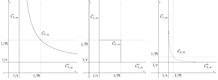
Figure 1. The first three curves in $\Sigma_{\infty}$ for a domain type I (left) and type II (middle and right).

5.1. Type I

Here lies the domain $\Omega$ whose curve $\mathcal{C}_{2,\infty}$ is hyperbolic and asymptotic to the trivial lines. As we have seen the only possibility is a ball.

Example 5.1 (A ball).

Let us consider the domain $\Omega$ given by a open ball of radius $R$ in $\mathbb{R}^{n}$. It is immediate that $\lambda_{1,\infty}(\Omega)=\frac{1}{R}$.

Since the radii of two tangential balls fitted in $\Omega$ must satisfy $r_{1}+r_{2}=R$, the expression of (4.2) will be minimized will be minimized when $\frac{t}{r_{1}}=\frac{1}{r_{2}}$, i.e.,

$$t=\frac{r_{1}}{R-r_{1}},\qquad\text{ which implies }\quad r_{1}=\frac{Rt}{1+t}.$$

In such case it follows that

$$c_{\infty}(t)=\frac{1+t}{R}.$$

Finally, observe that values of $t$ approaching zero correspond to a partition $(\omega_{1},\omega_{2})\in\mathcal{P}(\Omega)$ in which the biggest ball in $\omega_{2}$ is almost the whole $\Omega$ and the biggest one in $\omega_{1}$ is very small; values of $t$ approaching $+\infty$ correspond to a partition in which the balls interchange their roles: the biggest ball in $\omega_{1}$ is almost the whole $\Omega$. See figure 2.

Consequently, according equation (1.9), the curve $\mathcal{C}_{2,\infty}$ is given by

$$\mathcal{C}_{2,\infty}=\left\{\left(\frac{1+t}{Rt},\frac{1+t}{R}\right),\,t\in\mathbb{R}^{+}\right\}.$$

Observe that when $t=1$ the curve contains the point $\left(\frac{2}{R},\frac{2}{R}\right)$, which is precisely corresponds to $(\lambda_{2,\infty}(\Omega),\lambda_{2,\infty}(\Omega))$.

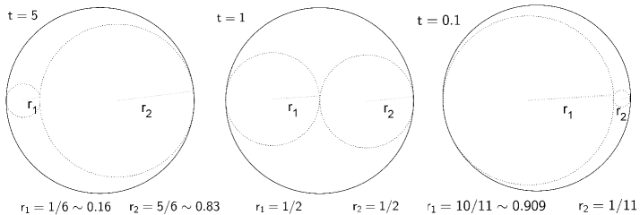
Figure 2. Partitions corresponding to $t=1$ ($r_{1}\sim 0.16$ and $r_{2}\sim 0.83$), $t=1$ ($r_{1}=r_{2}=0.5)$ and $t=0.1$ ($r_{1}\sim 0.909$ and $r_{2}\sim 0.09$)

for $\Omega$ the unit ball .

Example 5.2 (The unit interval).

When $\Omega$ is considered to be an open interval in the real line, the picture of $\Sigma_{\infty}$ is analogous to $\Sigma_{p}$ for a fixed value of $p$, i.e., it consists in a sequence of hyperbolic-like curves, as it is showed in Figure 3.

Moreover, since explicit formulas for the eigenfunctions are known for a fixed value of $p$, it is possible to describe the profile of the limit problem. For instance, if $(\alpha,\beta)\in\mathcal{C}_{2,\infty}$, the corresponding eigenfunction $u_{\infty}$ will be given by

$$\lim_{p\to\infty}u_{p}(x)=u_{\infty}(x)=\begin{cases}x&\quad\text{in }\left(0,\frac{\ell}{2}\right]\\ -x+\ell&\quad\text{in }\left[\frac{\ell}{2},\frac{\ell+1}{2}\right]\\ x-1&\quad\text{in }\left[\frac{\ell+1}{2},1\right)\end{cases}$$

where $\ell\in(0,1)$ and

$$u_{p}(x)=\begin{cases}\displaystyle\sin_{p}\left(\frac{\pi_{p}x}{\ell}\right)&\quad\text{in }(0,\ell]\\ \displaystyle-\sin_{p}\left(\frac{\pi_{p}x}{1-\ell}\right)&\quad\text{in }[\ell,1).\end{cases}$$

Finally, notice that $u_{\infty}$ is a viscosity solution to (1.8) with $(\alpha(l),\beta(l))=\left(\frac{2}{l},\frac{2}{1-l}\right)$.

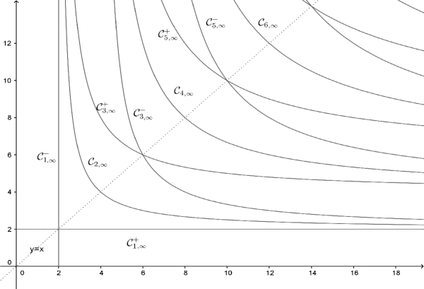
Figure 3. $\Sigma_{\infty}$ for the unit interval in $\mathbb{R}$.

5.2. Type II

All domain $\Omega$ whose curve $\mathcal{C}_{2,\infty}$ intersects the trivial lines. We can also subdivide this category in $\mathcal{C}_{2,\infty}$ connecting the trivial lines (type II.A) and $\mathcal{C}_{2,\infty}$ totally contained in the trivial lines (type II.B).

Example 5.3 (“Linked” balls).

Given $R_{1}\leq R_{2}$, let us consider a domain $\Omega$ made as the union of the balls of radii $R_{1}$ and $R_{2}$ by means of a tube of length $\varepsilon<R_{1}$.

Since the radius of the biggest ball contained in $\Omega$ is $R_{2}$, we get $\lambda_{1,\infty}=\frac{1}{R_{2}}$. Now, the couple of biggest balls contained in $\Omega$ have radius $R_{1}$. If we fix $r$ such that $r=R_{1}$, the expression of $c_{\infty}$ will be minimized when $\frac{t}{r}=\frac{1}{R_{1}}$, that is, when both coefficients inside the maximum in the expression of $c_{\infty}$ are the same. In this case, $c_{\infty}=\frac{1}{R_{1}}$.

Observe that the case $r=R_{1}$, corresponds to $t=1$. As $r$ increases, the value of $t$ decreases. This process finishes when $r=R_{2}$, which corresponds to $t=\frac{R_{2}}{R_{1}}$.

Analogously, this process can be made interchanging the roles of $R_{1}$ and $R_{2}$, leading to the following expression for the second non-trivial curve

$$\mathcal{C}_{2,\infty}=\left\{\left(\frac{1}{tR_{1}},\frac{1}{R_{1}}\right),\,1\leq t\leq\frac{R_{2}}{R_{1}}\right\}\cup\left\{\left(\frac{1}{R_{1}},\frac{1}{tR_{1}}\right),\,1\leq t\leq\frac{R_{2}}{R_{1}}\right\}.$$

It is remarkable to see that in the extremal case $R_{1}=R_{2}$ the curve $\mathcal{C}_{2,\infty}$ is contained in the trivial curves. This situation occurs when the radius of the biggest ball contained in $\Omega$ coincides with the radius of biggest couple of balls of the same size fitted in $\Omega$ (for example in an annular domain or more generally in a stadium domain).

It is also straightforward to see that the analysis made above only depends of radius of the biggest ball contained in $\Omega$ and the radius of biggest couple of identical balls contained in $\Omega$. Consequently, the three domains exhibited in figure 4 have the same first curves $\mathcal{C}_{1,\infty}^{\pm}$ and $\mathcal{C}_{2,\infty}$.

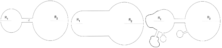
Figure 4. Three domains for which the first three curves in $\Sigma_{\infty}$ coincide.

Example 5.4 (The unit cube).

Let us consider $\Omega$ be the unit square in $\mathbb{R}^{2}$, $\Omega=(0,1)\times(0,1)$. In this case, since the biggest ball fitted in $\Omega$ has radius $R=\frac{1}{2}$ we have that $\lambda_{1,\infty}(\Omega)=2$.

Let us analyze the second nontrivial curve. When we compute $c_{\infty}(t)$ we must consider two balls of radii $r_{1}$ and $r_{2}$ contained in $\Omega$ such that $\frac{t}{r_{1}}$ and $\frac{1}{r_{2}}$ coincide. Notice that for $t=1$ we obtain

$$r_{1}=r_{2}=\frac{\sqrt{2}}{2(1+\sqrt{2})}.$$

But we can also consider a partition such that $r_{2}$ increases and $r_{1}$ decreases; since both balls are fitted in $\Omega$, they must verify

$$r_{1}+r_{2}=\frac{\sqrt{2}}{1+\sqrt{2}}.$$

In this case, if

$$t=\frac{1}{r_{1}}\frac{\sqrt{2}}{1+\sqrt{2}}-1$$

we can guarantee that $\frac{t}{r_{1}}$ and $\frac{1}{r_{2}}$ coincide. Observe that the computations made to enlarge $r_{1}$ (and then to obtain a smaller $r_{2}$) with the previous expression of $t$ can be performed provided that $r_{1}\leq\frac{1}{2}$. This procedure gives that

(5.1) $$c_{\infty}(t)=\frac{t}{r_{1}}=\frac{1}{r_{2}}=(t+1)\Big{(}1+\frac{\sqrt{2}}{2}\Big{)},\qquad\frac{2\sqrt{2}}{1+\sqrt{2}}-1\leq t\leq 1.$$

Now we can fix the value $r_{2}=\frac{1}{2}$ to be the maximum radius of a ball fitted in $\Omega$ and to continue decreasing the value of $r_{1}$. In this case, when considering

$$t=2r_{1}$$

we can assure that $\frac{t}{r_{1}}$ and $\frac{1}{r_{2}}$ coincides to be equal to $2$. This process can be continued as $r_{2}\to 0$ obtaining

(5.2) $$c_{\infty}(t)=2,\qquad 0\leq t\leq\frac{2\sqrt{2}}{1+\sqrt{2}}-1.$$

From (5.1) and (5.2) we get that

$$\mathcal{C}_{2,\infty}^{1}=\left\{\begin{array}[]{ll}\displaystyle\left(\frac{2}{t},2\right)&\displaystyle\qquad 0\leq t\leq\frac{2\sqrt{2}}{1+\sqrt{2}}-1\\ \displaystyle\left(\frac{\tau(t+1)}{t},\tau(t+1)\right)&\displaystyle\qquad\frac{2\sqrt{2}}{1+\sqrt{2}}-1\leq t\leq 1\end{array}\right.$$

where $\tau=1+\frac{\sqrt{2}}{2}$.

Observe that this construction can be made, analogously, interchanging the roles of $r_{1}$ and $r_{2}$, leading to

$$\mathcal{C}_{2,\infty}^{2}=\left\{\begin{array}[]{ll}\displaystyle\left(2,\frac{2}{t}\right)&\qquad\displaystyle 0\leq t\leq\frac{2\sqrt{2}}{1+\sqrt{2}}-1\\ \displaystyle\left(\tau(t+1),\frac{\tau(t+1)}{t}\right)&\displaystyle\qquad\frac{2\sqrt{2}}{1+\sqrt{2}}-1\leq t\leq 1,\end{array}\right.$$

and consequently, $\mathcal{C}_{2,\infty}=\mathcal{C}_{2,\infty}^{1}\cup\mathcal{C}_{2,\infty}^{2}$. See Figure 5.

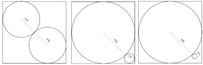
Figure 5. Partitions corresponding to $\Omega$ the unit cube in $\mathbb{R}^{2}$ for $t=1$, i.e., $r_{1}=r_{2}=\frac{\sqrt{2}}{2(1+\sqrt{2})}$ (left); $t=\frac{2\sqrt{2}}{1+\sqrt{2}}$, i.e., $r_{2}=\frac{1}{2}$, $r_{1}=\frac{\sqrt{2}}{1+\sqrt{2}}-\frac{1}{2}$ (middle) and $t=0.16$ with $r_{2}=\frac{2\sqrt{2}}{1+\sqrt{2}}$ and $r_{1}=0.08$ (right)

It is remarkable to see that for values of $t$ in the range $[0,\frac{2\sqrt{2}}{1+\sqrt{2}}-1]$, the curve $C_{2,\infty}$ is contained in the trivial lines, i.e., the first intersection among the second nontrivial curve and the trivial lines occurs at $(\tau_{0},2)$ and $(2,\tau_{0})$, where $\tau_{0}=\frac{2(\sqrt{2}+1)}{\sqrt{2}-1}$. See Figure 6.

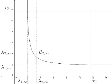
Figure 6. The curve $C_{2,\infty}$ for the unit cube in $\mathbb{R}^{2}$.

Acknowledgments This work has been partially supported by Consejo Nacional de Investigaciones Científicas y Técnicas (CONICET-Argentina). JVS would like to thank the Dept. of Math. FCEyN, Universidad de Buenos Aires for providing an excellent working environment and scientific atmosphere during his Postdoctoral program.

References

- [1] A. Anane, Simplicité et isolation de la première valeur propre du -laplacien avec poids, C. R. Acad. Sci. Paris Sér. I Math. 305 (1987), no. 16, 725–728.
- [2] M. Belloni and B. Kawohl, The pseudo--Laplace eigenvalue problem and viscosity solutions as , ESAIM Control Optim. Calc. Var. 10 (2004), no. 1, 28–52.
- [3] T. Bhattacharya, E. DiBenedetto, and J. Manfredi, Limits as of and related extremal problems, Rend. Sem. Mat. Univ. Politec. Torino (1989), no. Special Issue, 15–68 (1991), Some topics in nonlinear PDEs (Turin, 1989).
- [4] T. Champion, L. De Pascale, and C. Jimenez, The -eigenvalue problem and a problem of optimal transportation, Commun. Appl. Anal. 13 (2009), no. 4, 547–565
- [5] M. Conti, S. Terracini, and G. Verzini, On a class of optimal partition problems related to the Fučík spectrum and to the monotonicity formulae, Calc. Var. Partial Differential Equations 22 (2005), no. 1, 45–72.
- [6] M. G. Crandall, H. Ishii, and P.-L. Lions, User’s guide to viscosity solutions of second order partial differential equations, Bull. Amer. Math. Soc. (N.S.) 27 (1992), no. 1, 1–67.
- [7] G. Crasta and I. Fragalà, Rigidity results fro variational infinity ground states, Preprint arXiv:1702.01043v.
- [8] M. Cuesta, D. de Figueiredo, and J.-P. Gossez, The beginning of the Fučik spectrum for the -Laplacian, J. Differential Equations 159 (1999), no. 1, 212–238.
- [9] M. Cuesta, D. de Figueiredo, and J.-P. Gossez, Sur le spectre de Fučik du -Laplacien, C. R. Acad. Sci. Paris Sér. I Math. 326 (1998), no. 6, 681–684.
- [10] M. Cuesta and J.-P. Gossez, A variational approach to nonresonance with respect to the Fučik spectrum, Nonlinear Anal. 19 (1992), no. 5, 487–500.
- [11] E. N. Dancer, On the Dirichlet problem for weakly non-linear elliptic partial differential equations, Proc. Roy. Soc. Edinburgh Sect. A 76 (1976/77), no. 4, 283–300.
- [12] by same author, Generic domain dependence for nonsmooth equations and the open set problem for jumping nonlinearities, Topol. Methods Nonlinear Anal. 1 (1993), no. 1, 139–150.
- [13] D. de Figueiredo and J.-P. Gossez, On the first curve of the Fučik spectrum of an elliptic operator, Differential Integral Equations 7 (1994), no. 5-6, 1285–1302.
- [14] P. Drábek, Solvability and bifurcations of nonlinear equations, Pitman Research Notes in Mathematics Series, vol. 264, Longman Scientific & Technical, Harlow; copublished in the United States with John Wiley & Sons, Inc., New York, 1992.
- [15] G. Franzina and G. Palatucci, Fractional -eigenvalues, Riv. Math. Univ. Parma (N.S.) 5 (2014), no. 2, 373–386.
- [16] S. Fučík and A. Kufner, Nonlinear differential equations, Studies in Applied Mechanics, vol. 2, Elsevier Scientific Publishing Co., Amsterdam-New York, 1980.
- [17] S. Fucik, Solvability of nonlinear equations and boundary value problems, Mathematics and its Applications, vol. 4, D. Reidel Publishing Co., Dordrecht-Boston, Mass., 1980, With a foreword by Jean Mawhin.
- [18] J. P. García Azorero and I. Peral Alonso, Existence and nonuniqueness for the -Laplacian: nonlinear eigenvalues, Comm. Partial Differential Equations 12 (1987), no. 12, 1389–1430.
- [19] S. Goyal and K. Sreenadh, On the Fučik spectrum of non-local elliptic operators, NoDEA Nonlinear Differential Equations Appl. 21 (2014), no. 4, 567–588.
- [20] R. Hynd, C.K. Smart, and Y. Yu, Nonuniqueness of infinity ground states, Calc. Var. Partial Differential Equations 48 (2013), no. 3-4, 545–554.
- [21] P. Juutinen and P. Lindqvist, On the higher eigenvalues for the -eigenvalue problem, Calc. Var. Partial Differential Equations 23 (2005), no. 2, 169–192.
- [22] P. Juutinen, P. Lindqvist, and J. J. Manfredi, The -eigenvalue problem, Arch. Ration. Mech. Anal. 148 (1999), no. 2, 89–105.
- [23] E. Lindgren and P. Lindqvist, Fractional eigenvalues, Calc. Var. Partial Differential Equations 49 (2014), no. 1-2, 795–826.
- [24] A. M. Micheletti, A remark on the resonance set for a semilinear elliptic equation, Proc. Roy. Soc. Edinburgh Sect. A 124 (1994), no. 4, 803–809.
- [25] J. C. Navarro, J.D. Rossi, A. San Antolin, and N. Saintier, The dependence of the first eigenvalue of the infinity Laplacian with respect to the domain, Glasg. Math. J. 56 (2014), no. 2, 241–249.
- [26] K. Perera, On the Fučík spectrum of the -Laplacian, NoDEA Nonlinear Differential Equations Appl. 11 (2004), no. 2, 259–270.
- [27] K. Perera and M. Schechter, Type II regions between curves of the Fučík spectrum and critical groups, Topol. Methods Nonlinear Anal. 12 (1998), no. 2, 227–243.
- [28] by same author, The Fučík spectrum and critical groups, Proc. Amer. Math. Soc. 129 (2001), no. 8, 2301–2308.
- [29] K. Perera, M. Squassina and Y. Yang. A note on the Dancer-Fučík spectra of the fractional -Laplacian and Laplacian operators, Adv. Nonlinear Anal. 4(1) (2015) 13–23.
- [30] M. Schechter, The Fučík spectrum, Indiana Univ. Math. J. 43 (1994), no. 4, 1139–1157.
- [31] Y. Yu, Some properties of the ground states of the infinity Laplacian, Indiana Univ. Math. J. 56 (2007), 947–964.