Universal horizons and Hawking radiation in nonprojectable 2d Hořava gravity coupled with a non-relativistic scalar field

Abstract

In this paper, we study the non-projectable 2d Hořava gravity coupled with a non-relativistic scalar field, where the coupling is in general non-minimal and of the form $f(\phi)R$, where $f(\phi)$ is an arbitrary function of the scalar field $\phi$, and $R$ denotes the 2d Ricci scalar. In particular, we first investigate the Hamiltonian structure, and show that there are two-first and two-second class constraints, similar to the pure gravity case, but now the local degree of freedom is one, due to the presence of the scalar field. Then, we present various exact stationary solutions of this coupled system, and find that some of them represent black holes but now with universal horizons as their boundaries. At these horizons, the Hawking radiations are thermal with temperatures proportional to their surface gravities, which normally depend on the non-linear dispersion relations of the particles radiated, similar to the (3+1)-dimensional case.

I Introduction

Quantization of gravity is a subject of intense study over half a century QGs , and various candidates have been proposed, such as string/M-Theory strings , Loop Quantum Gravity (LQG) LQGs , Causal Dynamical Triangulation (CDT) CDTs , and Asymptotic Safety ASs , to name only a few of them. For more details, see Bojowald15 . However, our understanding on each of them is still highly limited. In particular, it is not clear how they are related (if there exists any), and which is the theory we have been looking for over these years. One of the main reasons is the absence of experimental evidences for quantum gravitational effects. In certain senses, this is understandable, considering the fact that quantum gravitational effects are normally expected to become important only at the Planck scale, which currently is well above the range of any man-made terrestrial experiments. However, the situation has been changing recently with the arrival of precision cosmology KWs . Particularly, it was shown lately that one of the approaches adopted in loop quantum cosmology already leads to inconsistency with current observations under certain circumstances Grain16 .

It is well known that general relativity is perturbatively not renormalizable, and its ultraviolet (UV) behavior can be dramatically changed by including high-order derivative operators, such as the term $R_{\mu\nu}R^{\mu\nu}$ Stelle , where $R_{\mu\nu}$ denotes the four-dimensional Ricci tensor. However, the inclusion of such terms inevitably leads to the presence of ghosts, which makes the theory not unitary Stelle . This problem has been plagued there since its discovery, and has not been resolved so far. The existence of the ghosts is closely related to the fact that the theory now contains time-derivatives with orders higher than two. As a matter of fact, there exists a powerful theorem due to Mikhail Vasilevich Ostrogradsky, who established it in 1850 Ostrogradsky . The theorem basically states that a system is not (kinematically) stable if it is described by a non-degenerate higher-order time-derivative Lagrangian. For a recent introduction of this theorem, we refer readers to Woodard15 .

To avoid the Ostrogradsky ghost problem, Hořava recently proposed a theory of gravity Horava , in which Lorentz invariance (LI) is broken in the UV but recovered (approximately) later in the infrared (IR). Once LI is broken, one can include only high-order spatial derivative operators into the Lagrangian, so the UV behavior can be dramatically improved, while the time derivative operators are still kept to the second-order, in order to evade Ostrogradsky’s ghosts and keep the theory unitary. There are many ways to break LI. But, Hořava chose to break it by considering anisotropic scaling between time and space,

$$t\rightarrow b^{-z}t,\;\;\;x^{i}\rightarrow b^{-1}{x}^{i},\;(i=1,2,...,d)$$ (1.1)

where $z$ denotes the dynamical critical exponent, and LI requires $z=1$, while power-counting renomalizibality requires $z\geq d$, where $d$ denotes the spatial dimension of the spacetime Horava ; Visser . Clearly, such a scaling breaks explicitly the LI and hence $4$-dimensional diffeomorphism invariance. Hořava assumed that it is broken only down to the level

$$t\to\xi_{0}(t),\quad{x}^{i}\to\xi^{i}\left(t,x^{k}\right),$$ (1.2)

so the spatial diffeomorphism still remains. The above symmetry is often referred to as the foliation-preserving diffeomorphism, denoted by Diff(M, ${\cal{F}}$). In the original incarnation of Hořava gravity Horava , the theory suffered several problems, including instability in the IR, strong coupling and inconsistency with observations LMP . Since then, various modifications have been proposed, and for a recently updated review we refer readers to Wang17 .

Among several important issues, quantization of Hořava gravity has been considered only in some particular cases, despite the vast literature on the theory. In particular, in (3+1)-dimensional spacetimes with the projectability and detailed balance conditions, the renormalizability of Hořava gravity was shown to reduce to the one of the corresponding (2+1)-dimensional topologically massive gravity OR09 . The latter is expected to be renormalizable DY90 , although a rigorous proof is still absent. Lately, it was shown that the theory is renormalizable even without the detailed balance condition, by properly choosing a gauge that ensures the correct anisotropic scaling of the propagators and their uniform falloff at large frequencies and momenta BBHSS .

Along a similar line, together with their collaborators, two of the current authors studied the quantization of Hořava gravity both with and without the projectability condition in (1+1)-dimensional (2D) spacetimes Li14 ; Li16 . Due to the foliation-preserving diffeomorphism, the theory is non-trivial even in 2d spacetimes, in contrast to the relativistic case Jackiw85 ; Brown88 ; GKV02 , although the total degree of freedom of the theory is still zero Li14 ; Li16 . In particular, in the projectable case, when only gravity is present, the system can be quantized by following the canonical Dirac quantization Dirac64 , and the corresponding wavefunction is normalizable Li14 . It is remarkable to note that in this case the corresponding Hamilton can be written in terms of a simple harmonic oscillator, whereby the quantization can be carried out quantum mechanically in the standard way. When minimally coupled to a scalar field, the momentum constraint can be solved explicitly in the case where the fundamental variables are functions of time only. In this case, the coupled system can also be quantized by following the Dirac process, and the corresponding wavefunction is also normalizable.

In the non-projectable case, the analysis of the 2D Hamiltonian structure shows that there are two first-class and two second-class constraints Li16 . Then, following Dirac one can quantize the theory by first requiring that the two second-class constraints be strongly equal to zero, which can be carried out by replacing the Poisson bracket by the Dirac bracket Dirac64 . The two first-class constraints give rise to the Wheeler-DeWitt equations. A remarkable feature is that orderings of the operators from a classical Hamilton to a quantum mechanical one play a fundamental role in order for the Wheeler-DeWitt equation to have nontrivial solutions. In addition, the space-time is well quantized, even when it is classically singular.

Moreover, it was also shown that the 2d projectable Hořava gravity is exactly equal to the 2d CDT AGSW . Such studies were further generalized to the case coupled with a scalar field AGJZ . In addition, the quantization of 2d Friedmann-Robertson-Walker universe was studied in VB16 ; Pitelli16 .

In this paper, we continue our investigations in 2d Hořava gravity with the non-projectable condition, but focus ourselves on two related issues: the existence of universal horizons and their Hawking radiations. The existence of black holes in gravitational theories with LI is closely related to the existence of light-cones HE73 . Then, in theories in which LI is broken, it was expected that black holes should not exist, as particles in such theories can have speeds larger than that of light, and such particles are always able to cross event horizons to escape to infinity, even they are trapped inside them initially. Therefore, it was very surprised to discover that black holes exist even in such theories, but now with universal horizons as the boundaries of black holes BS11 ; BJS , instead of Killing horizons HE73 .

Since then, universal horizons and their thermodynamics have been studied intensively (See, for example, Wang17 and references therein). In particular, it was showed that universal horizons exist in the three well-known black hole solutions: the Schwarzschild, Schwarzschild anti-de Sitter, and Reissner-Nordström LGSW , which are also solutions of Hořava gravity GLLSW . At the universal horizon, the first law of black hole mechanics exists for the neutral Einstein-aether black holes BBMa , provided that the surface gravity is defined by CLMV ,

$$\kappa_{UH}\equiv\frac{1}{2}u^{\alpha}D_{\alpha}\left(u_{\lambda}\zeta^{\lambda}\right),$$ (1.3)

which was obtained by considering the peering behavior of ray trajectories of constant khronon field $\phi$. However, for the charged Einstein-aether black holes, such a first law is still absent DWW . The universal horizon radiates as a blackbody at a fixed temperature BBMb . However, different species of particles, in general, experience different temperatures DWWZ ,

$$T_{UH}^{z\geq 2}=\frac{2(z-1)}{z}\left(\frac{\kappa_{UH}}{2\pi}\right),$$ (1.4)

where $\kappa_{UH}$ is the surface gravity calculated from Eq.(1.3) and $z$ is the exponent of the dominant term in the UV. When $z=2$ we have the standard result, $T_{UH}^{z=2}=\frac{\kappa_{UH}}{2\pi}$, which was first obtained in BBMb ; CLMV .

Recently, more careful studies of ray trajectories showed that the surface gravity for particles with a non-relativistic dispersion relation is indeed given by DL16 ,

$$\kappa_{UH}^{z\geq 2}=\frac{2(z-1)}{z}\kappa_{UH}.$$ (1.5)

The same results were also obtained in Cropp16 . It is remarkable to note that in terms of $\kappa_{UH}^{z\geq 2}$ and $T_{UH}^{z\geq 2}$, the standard relationship between the temperature and surface gravity of a black hole still holds here.

In this paper, we shall study universal horizons and their thermodynamics in 2d non-projectable Hořava gravity, coupled with a non-relativistic scalar field. Specifically, the paper is organized as follows: In Sec. II, we present the general action of the coupled system and derive the corresponding Hamiltonian structure and field equations. In Sec. III, we find various diagonal and non-diagonal stationary solutions of the coupled system, and correct some typos presented in BBC15 . In Sec. IV we first study the existence of universal horizons in a representative spacetime found in Sec. III, and then study its Hawking radiation by using the Hamilton-Jacobi method. To compare it with the relativistic case, Hawking radiation at Killing horizons is also studied in this section. The paper is ended in Sec. V, in which we present our main conclusions.

Before proceeding further, we would like to note that the existence of universal horizons is closely related to the existence of a globally defined time-like khronon field $\varphi$ Wang17 . Then, all the particles are assumed to move in the increasing direction of $\varphi$. At the beginning, universal horizons were studied in the framework of the Einstein-aether theory with spherical symmetry, in which the time-like aether naturally plays the role of the khronon field BS11 ; BJS . To generalize such conceptions to other theories, including Hořava gravity, in which the aether field is not part of the theory, one can consider the khronon field as a test field LACW , a role similar to a Killing vector field $\xi_{\mu}$, which satisfies the Killing equations, $\nabla_{(\nu}\xi_{\mu)}=0$, on a given spacetime background $g_{\mu\nu}$. In this paper, we shall adopt this generalization, and assume that the test khronon field satisfies the same equations as the aether field, the most general second-order partial differential equations in terms of the aether four-velocity JM01 . For more detail, we refer readers to Wang17 and references therein.

II 2d Hořava gravity coupled with a scalar field

The general gravitational action of Hořava gravity is given by,

$$S_{HL}=\zeta^{2}\int{dt\,dx\,N\sqrt{g}\left({\cal{L}}_{K}-{\cal{L}}_{V}\right)},$$ (2.1)

where $\zeta^{2}$ denotes the coupling constant of Hořava gravity, $N$ the lapse function in the Arnowitt-Deser-Misner (ADM) decomposition ADM , and $g\equiv{\mbox{det}}(g_{ij})$, here $g_{ij}$ is the spatial metric defined on the leaves $t=$ Constant. ${\cal{L}}_{K}$ is the kinetic part of the action, given by

$${\cal{L}}_{K}=K_{ij}K^{ij}-\lambda K^{2},$$ (2.2)

where $\lambda$ is a dimensionless constant, and $K_{ij}$ denotes the extrinsic curvature tensor of the leaves $t=$ constant, given by

$$K_{ij}=\frac{1}{2N}\left(-\dot{g}_{ij}+\nabla_{i}N_{j}+\nabla_{j}N_{i}\right),$$ (2.3)

and $K\equiv g^{ij}K_{ij}$. Here $\dot{g}_{ij}\equiv\partial{g}_{ij}/\partial t$, $\nabla_{i}$ denotes the covariant derivative of the metric $g_{ij}$, and $N^{i}$ the shift vector, with $N_{i}\equiv g_{ij}N^{j}$. ${\cal{L}}_{V}$ denotes the potential part of the action, and in 2d spacetimes, it takes the form Li16 ,

$${\cal{L}}_{V}=2\Lambda-\beta a_{i}a^{i},$$ (2.4)

where $\Lambda$ denotes the cosmological constant, and $\beta$ is another dimensionless coupling constant.

On the other hand, the action for a non-relativistic scalar field takes the form,

$$S_{\phi} = \int{dt\,dx\,N\sqrt{g}\Bigg{\{}\frac{1}{2}\left(\partial_{\perp}\phi\right)^{2}-\alpha_{0}\left(\nabla_{i}\phi\right)^{2}}$$ (2.5)

$$~{}~{}~{}~{}~{}~{}~{}~{}~{}~{}~{}~{}~{}~{}~{}~{}~{}~{}~{}~{}{-V(\phi)-f(\phi)R\Bigg{\}}},$$

where $\partial_{\perp}\equiv N^{-1}(\partial_{t}-N^{i}\nabla_{i})$, $\alpha_{0}$ is a dimensionless coupling constant. In the relativistic case, it is equal to $1/2$. The function $f(\phi)$ is arbitrary and depends on $\phi$ only, and $R$ denotes the Ricci scalar of the 2d spacetimes. The total action is

$$S=S_{HL}+S_{\phi}=\zeta^{2}\int{dt\,dx\,N\sqrt{g}{\cal{L}}}.$$ (2.6)

II.1 Hamiltonian Structure

The 2d spacetimes are described by the general metric,

$$ds^{2}=-N^{2}dt^{2}+\gamma^{2}\big{(}dx+N^{1}dt\big{)}^{2},$$ (2.7)

subjected to the gauge freedom (1.2), where $N,N^{1}$ and $\gamma$ are in general functions of $t$ and $x$. To be as much general as possible, we shall not impose any gauge conditions in this section. Then, the action (2.1) takes the form,

$$S_{HL}=\int{dtdxN\gamma\left[(1-\lambda)K^{2}-2{\Lambda}+\beta a_{1}a^{1}\right]}.$$ (2.8)

where $a_{1}=\left(\ln N\right)^{\prime}$, and

$$K=-\frac{1}{N}\left(\frac{\dot{\gamma}}{\gamma}-\frac{N^{\prime}_{1}}{\gamma^{2}}+\frac{N_{1}\gamma^{\prime}}{\gamma^{3}}\right),$$ (2.9)

with $\gamma^{\prime}\equiv\partial\gamma/\partial x$, etc. In terms of $N,N_{1}$ and $\gamma$, the matter action takes the form

$$S_{\phi} = \int dtdxN\gamma\left.\Big{\{}\frac{1}{2N^{2}}\left(\dot{\phi}-\frac{N_{1}\phi^{\prime}}{\gamma^{2}}\right)^{2}-\frac{\alpha_{0}}{\gamma^{2}}\phi^{\prime 2}\right.$$ (2.10)

$$\left.-V(\phi)-f(\phi)R\right.\Big{\}},$$

where

$$R=\frac{2}{N\gamma}\left[\partial_{\mu}(N\gamma n^{\mu}K)-\left(\frac{N^{\prime}}{\gamma}\right)^{\prime}\right].$$ (2.11)

Here $n^{\mu}\equiv N^{-1}(1,-N^{1})$ denotes the normal vector to the hypersurfaces $t=$ Constant. Then, we find

$$\pi_{N} \equiv \frac{\partial\mathcal{L}}{\partial\dot{N}}=0,\quad\pi_{N_{1}}\equiv\frac{\partial\mathcal{L}}{\partial\dot{N_{1}}}=0,$$

$$\pi = \frac{\partial\mathcal{L}}{\partial\dot{\gamma}}=2K(\lambda-1)-2f^{\prime}\frac{\dot{\phi}}{N}+2f^{\prime}\frac{\phi^{\prime}N_{1}}{N\gamma^{2}},$$

$$\pi_{\phi} = \frac{\partial\mathcal{L}}{\partial\dot{\phi}}=\frac{\gamma}{N}(\dot{\phi}-N_{1}\frac{\phi^{\prime}}{\gamma^{2}})+2f^{\prime}\gamma K.$$ (2.12)

After a Legendre transformation, it can be shown that the Hamiltonian can be cast in the form,

$$\mathcal{H}_{0}=N\mathcal{H}+N_{1}\mathcal{H}^{1}-2\beta\left(\frac{N^{\prime}}{\gamma}\right)^{\prime},$$ (2.13)

where

$$\mathcal{H}^{1} = -\frac{\pi^{\prime}}{\gamma}+\frac{\pi_{\phi}\phi^{\prime}}{\gamma^{2}},$$ (2.14)

$$\mathcal{H} = -\frac{\pi_{\phi}\pi}{2f^{\prime}}+\frac{(\lambda-1)\pi_{\phi}}{f^{\prime}}K+(1-\lambda)K^{2}\gamma$$ (2.15)

$$+2\Lambda\gamma+\alpha_{0}\frac{\phi^{\prime 2}}{\gamma}-\frac{\gamma}{2}\left(\frac{\pi_{\phi}}{\gamma}-2f^{\prime}K\right)^{2}$$

$$+\gamma V(\phi)-2\left(\frac{f^{\prime}\phi^{\prime}}{\gamma}\right)^{\prime}$$

$$+\beta\frac{N^{\prime 2}}{N\gamma}+2\beta\left(\frac{N^{\prime}}{N\gamma}\right)^{\prime}.$$

Here K can be expressed in terms of the canonical fields and their momenta,

$$K=\frac{\pi\gamma+2f^{\prime}\pi_{\phi}}{4\gamma f^{\prime 2}-2\gamma(1-\lambda)}.$$ (2.16)

A straightforward evaluation of poisson brackets between momentum constraints shows

$$\Big{\{}\mathcal{H}^{1}(x),\mathcal{H}^{1}(x^{\prime})\Big{\}}=\left(\frac{\mathcal{H}^{1}(x^{\prime})}{\gamma^{2}(x^{\prime})}+\frac{\mathcal{H}^{1}(x)}{\gamma^{2}(x)}\right)\partial_{x^{\prime}}\delta(x-x^{\prime}),$$ (2.17)

which is the same as in the pure gravity case Li16 . The poisson bracket between $\mathcal{H}$ and $\mathcal{H}^{1}$ will not vanish on the constraint surface because of the appearance of terms related to the lapse function $N$ in the Hamiltonian constraint $\mathcal{H}$. Therefore, we need to redefine the momentum constraint by adding a term proportional to the primary constraint $\pi_{N}$, which generates the diffeomorphisms of $N$,

$$\tilde{\mathcal{H}}^{1}=\mathcal{H}^{1}+\frac{N^{\prime}}{\gamma^{2}}\pi_{N}.$$ (2.18)

In principle, one can also add a term generating diffeomorphisms of $N_{1}$. However, in the present case, since the Hamiltonian constraint doesn’t depend on $N_{1}$, this term is not mandatory. In terms of $\tilde{\mathcal{H}}^{1}$, the structure of Eq.(2.17) will not change, while one can show that $\tilde{\mathcal{H}}^{1}$ now commutes with $\mathcal{H}$ on the constraint surface,

$$\Big{\{}\tilde{\mathcal{H}}^{1}(x),\mathcal{H}(x^{\prime})\Big{\}} = -\left(4\rm c\pi+\frac{2\rm{b}\pi_{\phi}}{\gamma}\right)\tilde{\mathcal{H}}^{1}(x)\delta(x-x^{\prime})$$ (2.19)

$$+\frac{\mathcal{H}(x)}{\gamma^{2}(x)}\partial_{x}\delta(x-x^{\prime}).$$

Here $\rm c\equiv-\alpha/2-2\xi^{2}\alpha^{2}$ and $\rm b\equiv\alpha\xi(2\beta-1)-\frac{1}{2\xi}[1+2\alpha(1-\lambda)]$, where $\alpha^{-1}\equiv 4\xi^{2}+2(\lambda-1)$. Note that in writing down the above expression, we had set $f(\phi)=\xi\phi$ for the sake of simplicity. Thus, the total Hamiltonian of the coupled system can be written as

$$\mathcal{H}_{t}=N\mathcal{H}+N_{1}\tilde{\mathcal{H}}^{1}+\sigma\pi_{N}+\sigma_{1}\pi_{N_{1}}.$$ (2.20)

For this coupled system, there are two first-class constraints $\tilde{\mathcal{H}}^{1}$ and $\pi_{N_{1}}$, and two second-class constraints $\mathcal{H}$ and $\pi_{N}$.

Note that no other constraints will be generated by the equations of motion (E.O.M.) of the said four constraints because the secondary constraint $\tilde{\mathcal{H}}^{1}$ will not give rise to any tertiary constraints due to Eqs.(2.17) and (2.19), while on the other hand the preservation of $\mathcal{H}$ will only produce two differential equations for lapse function $N$ and Lagrange multiplier $\sigma$ since $\mathcal{H}$ is a second-class constraint. Thus, the Dirac procedure of finding all the constraints in the Hamiltonian formulation terminates at the level of secondary constraints, and the physical degrees of freedom in the configuration space is one which is due to the introduction of the scalar field into the whole system, while in the pure gravity case it is zero Li16 .

II.2 Field Equations

The variations of the total action $S$ with respect to $N,N_{1},\gamma$ and $\phi$, yield, respectively,

$$(1-\lambda)\gamma K^{2}+2\beta\left(\frac{N^{\prime}}{N\gamma}\right)^{\prime}+\frac{\beta N^{\prime 2}}{N^{2}\gamma}+\gamma\left(2\Lambda+V\right)$$

$$~{}~{}~{}~{}~{}+\frac{\gamma}{2N^{2}}\left(\dot{\phi}-\frac{N_{1}\phi^{\prime}}{\gamma^{2}}\right)^{2}+\frac{\alpha_{0}\phi^{\prime 2}}{\gamma}$$

$$~{}~{}~{}~{}~{}+\frac{2K}{N}\left(f^{\prime}\dot{\phi}\gamma-\frac{f^{\prime}\phi^{\prime}N_{1}}{\gamma}\right)-\left(\frac{2f^{\prime}\phi^{\prime}}{\gamma}\right)^{\prime}=0,$$

$$\frac{2(1-\lambda)K^{\prime}}{\gamma}+\frac{\phi^{\prime}}{N\gamma}\left(\dot{\phi}-\frac{N_{1}\phi^{\prime}}{\gamma^{2}}\right)$$

$$~{}~{}~{}~{}~{}+\frac{2f^{\prime}\phi^{\prime}K}{\gamma}+\left(\frac{2f^{\prime}\dot{\phi}}{N\gamma}-\frac{2f^{\prime}\phi^{\prime}N_{1}}{N\gamma^{3}}\right)^{\prime}$$

$$~{}~{}~{}~{}~{}+\frac{2\gamma^{\prime}}{N\gamma^{3}}\left(f^{\prime}\dot{\phi}\gamma-\frac{f^{\prime}\phi^{\prime}N_{1}}{\gamma}\right)=0,$$ (2.22)

$$2(1-\lambda)\left(\dot{K}+\frac{N_{1}K^{\prime}}{\gamma^{2}}-\frac{NK^{2}}{2}\right)-\frac{\beta N^{\prime 2}}{N\gamma^{2}}$$

$$~{}~{}~{}~{}~{}+\frac{1}{2N}\left(\dot{\phi}-\frac{N_{1}\phi^{\prime}}{\gamma^{2}}\right)^{2}+\frac{2N_{1}\phi^{\prime}}{N\gamma^{2}}\left(\dot{\phi}-\frac{N_{1}\phi^{\prime}}{\gamma^{2}}\right)$$

$$~{}~{}~{}~{}~{}-N(2\Lambda+V)+2f^{\prime}\dot{\phi}K+2f^{\prime}\phi^{\prime}\frac{N_{1}K}{\gamma^{2}}$$

$$~{}~{}~{}~{}~{}+2f^{\prime}\phi^{\prime}\frac{N^{\prime}}{\gamma^{2}}+\alpha_{0}\phi^{\prime 2}\frac{N}{\gamma^{2}}-2K\left(f^{\prime}\dot{\phi}-\frac{f^{\prime}\phi^{\prime}N_{1}}{\gamma^{2}}\right)$$

$$~{}~{}~{}~{}~{}+\left(\frac{2f^{\prime}\dot{\phi}\gamma}{N\gamma}-\frac{2f^{\prime}\phi^{\prime}N_{1}}{N\gamma^{2}}\right)_{,t}$$

$$~{}~{}~{}~{}~{}-\frac{2N_{1}^{\prime}}{\gamma^{2}}\left(f^{\prime}\dot{\phi}\gamma-f^{\prime}\phi^{\prime}\frac{N_{1}}{\gamma}\right)$$

$$~{}~{}~{}~{}~{}+\frac{4N_{1}\gamma^{\prime}}{N\gamma^{4}}\left(f^{\prime}\dot{\phi}\gamma-f^{\prime}\phi^{\prime}\frac{N_{1}}{\gamma}\right)$$

$$~{}~{}~{}~{}~{}+\left(\frac{2N_{1}f^{\prime}\dot{\phi}}{N\gamma^{2}}-\frac{4f^{\prime}\phi^{\prime}N_{1}^{2}}{N\gamma^{4}}\right)^{\prime}=0,$$ (2.23)

$$\left(\frac{\gamma\dot{\phi}}{N}-\frac{N_{1}\phi^{\prime}}{N\gamma}\right)_{,t}-\left(\frac{N_{1}\dot{\phi}}{N\gamma}-\frac{N_{1}^{2}\phi^{\prime}}{N\gamma^{3}}\right)^{\prime}-2\alpha_{0}\left(\frac{N\phi^{\prime}}{\gamma}\right)^{\prime}$$

$$+N\gamma V^{\prime}-2f^{\prime\prime}\dot{\phi}\gamma K+2(f^{\prime}\gamma K)^{.}+2f^{\prime\prime}\phi^{\prime}\frac{N_{1}K}{\gamma}$$

$$-2\left(\frac{f^{\prime}N_{1}K}{\gamma}\right)^{\prime}+2f^{\prime\prime}\phi^{\prime}\frac{N^{\prime}}{\gamma}-2\left(\frac{f^{\prime}N^{\prime}}{\gamma}\right)^{\prime}=0.$$ (2.24)

Here $f^{\prime}(\phi)\equiv df(\phi)/d\phi$, etc. Note Eqs.(II.2)-(II.2) hold for any function $f(\phi)$.

III Stationary Spacetimes

In this section, we will study stationary spacetimes of the 2d Hořava gravity coupled with a non-relativistic scalar field, presented in the last section. Setting all the time derivative terms to zero in Eqs.(II.2)-(II.2), and

$$f(\phi)=\xi\phi,$$ (3.1)

where $\xi$ is a constant, we find that

$$(1-\lambda)\gamma K^{2}+2\beta\left(\frac{N^{\prime}}{N\gamma}\right)^{\prime}+\frac{\beta N^{\prime 2}}{N^{2}\gamma}+\frac{N_{1}^{2}\phi^{\prime 2}}{2N^{2}\gamma^{3}}$$

$$~{}~{}~{}~{}~{}~{}~{}~{}~{}~{}~{}~{}~{}~{}~{}+\frac{\alpha_{0}\phi^{\prime 2}}{\gamma}+\gamma(2\Lambda+V)-\frac{2K\xi\phi^{\prime}N_{1}}{N\gamma}$$

$$~{}~{}~{}~{}~{}~{}~{}~{}~{}~{}~{}~{}~{}~{}~{}-\left(\frac{2\xi\phi^{\prime}}{\gamma}\right)^{\prime}=0,$$ (3.2)

$$\frac{2(1-\lambda)K^{\prime}}{\gamma}-\frac{N_{1}\phi^{\prime 2}}{N\gamma^{3}}+\frac{2\xi\phi^{\prime}K}{\gamma}$$

$$~{}~{}~{}~{}~{}~{}~{}~{}~{}~{}~{}~{}~{}~{}~{}-\left(\frac{2\xi\phi^{\prime}N_{1}}{N\gamma^{3}}\right)^{\prime}-\frac{2\xi\phi^{\prime}\gamma^{\prime}N_{1}}{N\gamma^{4}}=0,$$ (3.3)

$$2(1-\lambda)\left(\frac{N_{1}K^{\prime}}{\gamma^{2}}-\frac{NK^{2}}{2}\right)-\frac{\beta N^{\prime 2}}{N\gamma^{2}}-\frac{3N_{1}^{2}\phi^{\prime 2}}{2N\gamma^{4}}$$

$$~{}~{}~{}~{}~{}~{}~{}~{}~{}~{}~{}~{}~{}~{}~{}+\alpha_{0}\phi^{\prime 2}\frac{N}{\gamma^{2}}+4\xi\phi^{\prime}\frac{N_{1}K}{\gamma^{2}}+2\xi\phi^{\prime}\frac{N^{\prime}}{\gamma^{2}}$$

$$~{}~{}~{}~{}~{}~{}~{}~{}~{}~{}~{}~{}~{}~{}~{}-N(2\Lambda+V)+\frac{2\xi N_{1}^{\prime}\phi^{\prime}N_{1}}{\gamma^{3}}$$

$$~{}~{}~{}~{}~{}~{}~{}~{}~{}~{}~{}~{}~{}~{}~{}-\frac{4\xi\gamma^{\prime}\phi^{\prime}N_{1}^{2}}{N\gamma^{5}}-\left(\frac{4\xi\phi^{\prime}N_{1}^{2}}{N\gamma^{4}}\right)^{\prime}=0,$$ (3.4)

$$\left(\frac{N_{1}^{2}\phi^{\prime}}{N\gamma^{3}}\right)^{\prime}-2\alpha_{0}\left(\frac{N\phi^{\prime}}{\gamma}\right)^{\prime}+N\gamma V^{\prime}$$

$$~{}~{}~{}~{}~{}~{}~{}~{}~{}~{}~{}~{}~{}~{}~{}-2\xi\left(\frac{N_{1}K}{\gamma}\right)^{\prime}-2\xi\left(\frac{N^{\prime}}{\gamma}\right)^{\prime}=0.$$ (3.5)

III.1 Diagonal Solutions

When the metric is diagonal, we have

$$N_{1}=0,$$ (3.6)

so the extrinsic curvature $K$ vanishes and Eq.(III) holds identically, while Eqs.(III), (III) and (III) reduce, respectively, to

$$2\beta\left(\nu^{\prime\prime}-\nu^{\prime}\mu^{\prime}\right)+{\beta}{\nu^{\prime}}^{2}-2\xi\left(\phi^{\prime\prime}-{\phi^{\prime}\mu^{\prime}}\right)+\alpha_{0}{\phi^{\prime}}^{2}$$

$$~{}~{}~{}~{}~{}~{}~{}~{}~{}~{}~{}~{}~{}~{}~{}~{}~{}~{}=-(V+2\Lambda)e^{2\mu},$$ (3.7)

$${\beta}{\nu^{\prime}}^{2}-2\xi{\phi^{\prime}\nu^{\prime}}-\alpha_{0}{\phi^{\prime}}^{2}=-(V+2\Lambda)e^{2\mu},$$ (3.8)

$$2\xi\left(\nu^{\prime\prime}+{\nu^{\prime}}^{2}-{\nu^{\prime}\mu^{\prime}}\right)+2\alpha_{0}\left(\phi^{\prime\prime}-{\phi^{\prime}\mu^{\prime}}+\nu^{\prime}\phi^{\prime}\right)$$

$$~{}~{}~{}~{}~{}~{}~{}~{}~{}~{}~{}~{}~{}~{}=e^{2\mu}V^{\prime},$$ (3.9)

where $\nu\equiv\ln N$ and $\mu\equiv\ln\gamma$.

It should be noted that static diagonal solutions were studied recently in BBC15 with $\Lambda=0=\xi$. However, comparing the above equation (III.1) with Eq.(12) given in BBC15 , it can be seen that the second-order derivative term $\nu^{\prime\prime}$ (or $N^{\prime\prime}$) is missing there. This is because, when taking the variation of the total action with respect to $N$, the authors of BBC15 incorrectly assumed that $a_{1}$ is independent of $N$. Unfortunately, as a result, all the solutions resulted from Eq.(12) given in BBC15 in general are not solutions of the field equations of the 2d Hořava gravity coupled with a non-relativistic scalar field.

Using the gauge freedom given by Eq.(1.2), without loss of the generality, we can always set $\mu=-\nu$, that is,

$$N=\frac{1}{\gamma}=e^{\nu}.$$ (3.10)

To solve Eqs.(III.1)-(III.1), let us further consider the case where $V=-2\Lambda$, so that Eqs.(III.1) - (III.1) reduce to,

$$2\beta\left(\nu^{\prime\prime}+{\nu^{\prime}}^{2}\right)+{\beta}{\nu^{\prime}}^{2}-2\xi\left(\phi^{\prime\prime}+{\phi^{\prime}\nu^{\prime}}\right)$$ (3.13)

$$~{}~{}~{}~{}~{}~{}~{}~{}~{}~{}~{}~{}~{}~{}~{}~{}~{}~{}+\alpha_{0}{\phi^{\prime}}^{2}=0,$$

$${\beta}{\nu^{\prime}}^{2}-2\xi{\phi^{\prime}\nu^{\prime}}-\alpha_{0}{\phi^{\prime}}^{2}=0,$$

$$\nu^{\prime\prime}+2{\nu^{\prime}}^{2}+\frac{\alpha_{0}}{\xi}\left(\phi^{\prime\prime}+2\nu^{\prime}\phi^{\prime}\right)=0.$$

Then, from Eqs.(3.13) and (3.13) we find that

$$\nu^{\prime\prime}+2{\nu^{\prime}}^{2}-\frac{\xi}{\beta}\left(\phi^{\prime\prime}+2\nu^{\prime}\phi^{\prime}\right)=0.$$ (3.14)

Thus, Eqs.(3.13) and (3.14) show that there are two possibilities,

$$(i)\;{\alpha_{0}}\beta+{\xi}^{2}\not=0;\quad(ii)\;{\alpha_{0}}\beta+{\xi}^{2}=0.$$ (3.15)

III.1.1 ${\alpha_{0}}\beta+{\xi}^{2}\not=0$

In this case we must have

$$\nu^{\prime\prime}+2{\nu^{\prime}}^{2}=0,$$ (3.16)

$$\phi^{\prime\prime}+2{\nu^{\prime}}\phi^{\prime}=0,$$ (3.17)

which have the solutions,

$$N = \sqrt{C_{0}x+C_{1}},$$

$$\phi = \phi_{0}\ln\left(C_{0}x+C_{1}\right)+\phi_{1},$$ (3.18)

where $C_{i}$ and $\phi_{i}$ are the integration constants. Without loss of the generality, we can always set $C_{0}=1$, so the metric and scalar field finally take the form,

$$ds^{2} = -\left(x-x_{0}\right)dt^{2}+\frac{dx^{2}}{x-x_{0}},$$

$$\phi = \phi_{0}\ln\left(x-x_{0}\right)+\phi_{1},$$ (3.19)

where $x_{0}\equiv-C_{1}$. Clearly, the scalar field is singular at $x=x_{0}$, so is the corresponding spacetime.

III.1.2 ${\alpha_{0}}\beta+{\xi}^{2}=0$

In this case, there are only two independent equations which are Eqs.(3.13) and (3.13). Now if substituting the relation $\alpha_{0}=-\xi^{2}/\beta$ into these equations and defining a new constant $\kappa=\xi/\beta$, one can easily arrive at,

$$\nu^{\prime 2}-2\kappa\phi^{\prime}\nu^{\prime}+\kappa^{2}\phi^{\prime 2} = 0,$$ (3.20)

$$\nu^{\prime\prime}+\nu^{\prime 2}-\kappa\phi^{\prime\prime}-\kappa^{2}\phi^{\prime 2} = 0.$$ (3.21)

The first equation tells us that $\nu^{\prime}$ and $\phi^{\prime}$ are linearly dependent, that is,

$$\nu=\frac{\xi}{\beta}\left(\phi-\phi_{0}\right),$$ (3.22)

which also makes the second equation hold identically, where $\phi_{0}$ is a constant. Therefore, in the current case for any chosen $\phi$, the solution (3.22) will satisfy the field equations (3.13)-(3.13). The corresponding metric takes the form,

$$ds^{2} = -e^{\frac{2\xi(\phi-\phi_{0})}{\beta}}dt^{2}+e^{-\frac{2\xi(\phi-\phi_{0})}{\beta}}dx^{2},$$ (3.23)

for ${\alpha_{0}}=-{\xi}^{2}/\beta$.

III.2 Non-diagonal Solutions

In this case, using the gauge transformations (1.2), without loss of generality, we can always set

$$\gamma=1,$$ (3.24)

so the metric takes the form,

$$ds^{2}=-N^{2}(x)dt^{2}+\big{(}dx+h(x)dt\big{)}^{2}.$$ (3.25)

Then, Eqs.(III)-(III) reduce to

$$(1-\lambda)K^{2}+2\beta\left(\frac{N^{\prime}}{N}\right)^{\prime}+\frac{\beta N^{\prime 2}}{N^{2}}+2\Lambda+V(\phi)+\frac{h^{2}\phi^{\prime 2}}{2N^{2}}$$

$$~{}~{}~{}~{}~{}~{}~{}~{}~{}+\alpha_{0}\phi^{\prime 2}-\frac{2K\xi\phi^{\prime}h}{N}-2\xi\phi^{\prime\prime}=0,$$ (3.26)

$$2(1-\lambda)K^{\prime}-\frac{h\phi^{\prime 2}}{N}+2\xi\phi^{\prime}K-\left(\frac{2\xi\phi^{\prime}h}{N}\right)^{\prime}=0,$$ (3.27)

$$2(1-\lambda)\left(hK^{\prime}-\frac{NK^{2}}{2}\right)-\frac{\beta N^{\prime 2}}{N}-\frac{3h^{2}\phi^{\prime 2}}{2N}$$

$$~{}~{}~{}~{}~{}~{}~{}~{}~{}-N(2\Lambda+V)+\alpha_{0}\phi^{\prime 2}N+4\xi\phi^{\prime}hK$$

$$~{}~{}~{}~{}~{}~{}~{}~{}~{}+2\xi\phi^{\prime}N^{\prime}+2\xi h^{\prime}\phi^{\prime}h-\left(\frac{4\xi\phi^{\prime}h^{2}}{N}\right)^{\prime}=0,$$ (3.28)

$$\left(\frac{h^{2}\phi^{\prime}}{N}\right)^{\prime}-2\alpha_{0}(N\phi^{\prime})^{\prime}+NV^{\prime}-2\xi(hK)^{\prime}-2\xi N^{\prime\prime}=0,$$

where

$$K=\frac{h^{\prime}}{N}.$$ (3.30)

To solve the above equations, in the following we shall consider some particular cases.

III.2.1 $N(x)=1$

In this case, let us first consider the solution with $\phi=\phi_{0}$, where $\phi_{0}$ is a constant. Then, from Eq.(III.2) we find that

$${h^{\prime}}^{2}=\frac{2\hat{\Lambda}}{\lambda-1},$$ (3.31)

where $\hat{\Lambda}\equiv\Lambda+V(\phi_{0})/2$. The above equation has the solution,

$$h(x)=\pm\sqrt{\frac{2\hat{\Lambda}}{\lambda-1}}\;x=\pm\eta x.$$ (3.32)

It can be shown that in this case a killing horizon exists, located at $x_{KH}=\pm\eta^{-1}$.

III.2.2 $\xi=0$

When $\xi=0$, Eqs.(III.2)-(III.2) reduces to

$$(1-\lambda)\left(\frac{h^{\prime}}{N}\right)^{2}+2\beta\left(\frac{N^{\prime}}{N}\right)^{\prime}+\frac{\beta N^{\prime 2}}{N^{2}}+\hat{V}$$

$$~{}~{}~{}~{}~{}~{}~{}~{}~{}+\alpha_{0}\phi^{\prime 2}+\frac{h^{2}\phi^{\prime 2}}{2N^{2}}=0,$$ (3.33)

$$2(1-\lambda)\left(\frac{h^{\prime\prime}}{N}-\frac{h^{\prime}N^{\prime}}{N^{2}}\right)-\frac{h\phi^{\prime 2}}{N}=0,$$ (3.34)

$$2(1-\lambda)\left(\frac{h^{\prime\prime}}{N}-\frac{h^{\prime}N^{\prime}}{N^{2}}-\frac{{h^{\prime}}^{2}}{2hN}\right)-\frac{\beta N^{\prime 2}}{hN}-\frac{3h\phi^{\prime 2}}{2N}$$

$$~{}~{}~{}~{}~{}~{}~{}~{}~{}+\frac{N}{h}\left(\alpha_{0}\phi^{\prime 2}-\hat{V}\right)=0,$$ (3.35)

$$\left(\frac{h^{2}\phi^{\prime}}{N}\right)^{\prime}-2\alpha_{0}(N\phi^{\prime})^{\prime}+N\hat{V}^{\prime}=0,$$ (3.36)

where $\hat{V}\equiv V+2\Lambda$. To solve the above equations, let us consider the case,

$$N=h,\quad\hat{V}=0,$$ (3.37)

for which the above equations reduce to

$$2\beta\nu^{\prime\prime}+(1-\lambda+\beta){\nu^{\prime}}^{2}=-\frac{1+2\alpha_{0}}{2}{\phi^{\prime}}^{2},$$ (3.38)

$$2(1-\lambda)\nu^{\prime\prime}={\phi^{\prime}}^{2},$$ (3.39)

$$2(1-\lambda)\nu^{\prime\prime}-(1-\lambda+\beta){\nu^{\prime}}^{2}=\frac{3-2\alpha_{0}}{2}{\phi^{\prime}}^{2},~{}~{}~{}~{}$$ (3.40)

$$(1-2\alpha_{0})\left(e^{\nu}\phi^{\prime}\right)^{\prime}=0,$$ (3.41)

where $\nu=\ln N$. To solve the above equations, let us consider the cases $\alpha_{0}=1/2$ and $\alpha_{0}\not=1/2$, separately.

Case B.2.1) $\alpha_{0}=1/2$: This is the relativistic case, and Eq.(3.41) is satisfied identically, while from Eqs.(3.38) and (3.40), we find

$$(1-\lambda+\beta)\nu^{\prime\prime}=0.$$ (3.42)

If $\lambda\not=\beta+1$, it can be shown that the above equations have only the trivial solution in which $\nu$ and $\phi$ are all constants. On the other hand, when $\lambda=\beta+1$, Eqs.(3.38)-(3.40) reduce to a single equation,

$$2\beta\nu^{\prime\prime}=-\phi^{\prime 2},\;(\beta=\lambda-1).$$ (3.43)

for the two arbitrary functions $\nu$ and $\phi$. Again, similar to Case A.2 considered in the last subsection, the solutions are not uniquely determined. In fact, for any given $\phi$, the solution,

$$\nu(x)=-\frac{1}{2\beta}\int^{x}{dx^{\prime}\int^{x^{\prime}}{{\phi^{\prime}}^{2}(x^{\prime\prime})dx^{\prime\prime}}}+C_{1}x+C_{0},$$ (3.44)

will satisfy the field equations (3.38) and (3.40), where $C_{1}$ and $C_{0}$ are two integration constants.

Case B.2.2) $\alpha_{0}\not=1/2$: In this case, from Eq.(3.41) we find

$$\phi^{\prime}=C_{0}e^{-\nu},$$ (3.45)

where $C_{0}$ is another constant. Substituting it into Eq.(3.39), we obtain

$$NN^{\prime\prime}-N^{\prime 2}+{\cal{D}}=0,$$ (3.46)

where ${\cal{D}}\equiv{C_{0}^{2}}/({2(\lambda-1)})$. The above equation has two particular solutions,

$$N_{A}(x) = \frac{1}{2C_{1}^{2}}e^{C_{1}(x+C_{2})}-\frac{{\cal{D}}}{2}e^{-C_{1}(x+C_{2})},$$ (3.47)

$$N_{B}(x) = \frac{1}{2C_{1}^{2}}e^{-C_{1}(x+C_{2})}-\frac{{\cal{D}}}{2}e^{C_{1}(x+C_{2})},$$ (3.48)

where $C_{1}$ and $C_{2}$ are two integration constants. Correspondingly, the scalar field $\phi$ is given, respectively, by,

$$\phi_{A}(x) = -\frac{2}{\sqrt{{\cal{D}}}}\tanh^{-1}\left(\frac{e^{C_{1}(C_{2}+x)}}{\sqrt{{\cal{D}}}C_{1}}\right),$$ (3.49)

$$\phi_{B}(x) = \frac{2}{\sqrt{{\cal{D}}}}\tanh^{-1}\left(C_{1}\sqrt{\cal{D}}e^{C_{1}(C_{2}+x)}\right).$$ (3.50)

IV Universal Horizons and Hawking Radiation

In this section, we shall consider two issues, universal horizons and the corresponding Hawking radiations. As a representative case, we shall focus on the solution given by Eqs.(3.25) and (3.32) with $N=1$. Without loss of the generality, we consider only the case with “-” sign, that is,

$$ds^{2} = -dt^{2}+\left(dx-\eta xdt\right)^{2}$$ (4.1)

$$= -\left(1-\eta^{2}x^{2}\right)dt^{2}-2\eta xdtdx+dx^{2},$$

where $-\infty<t,x<\infty$. The corresponding inverse metric is given by

$$g^{tt}=-1,\;\;\;g^{tx}=-\eta x,\;\;\;g^{xx}=1-\eta^{2}x^{2},$$ (4.2)

which is non-singular, except at the infinities $x=\pm\infty$. The latter are coordinate singularities, similar to the 4d de Sitter space. In fact, the extrinsic curvature and 2d Ricci scalar are all finite, and given by $-\eta$ and $2\eta^{2}$, respectively. However, there exist two cosmological Killing horizons, located, respectively, at $x_{KH}=\pm\eta^{-1}$. Similar to the 4d de Sitter space, the time-translation Killing vector, $\xi^{\mu}=\delta^{\mu}_{t}$, is time-like only in the region $x^{2}<x_{KH}^{2}$. In the regions $x^{2}>x_{KH}^{2}$, the Killing vector becomes spacelike, and only in these regions can the universal horizon exist, as the latter is defined by Wang17 ,

$$(\xi\cdot u)=0.$$ (4.3)

Since the four-velocity $u$ of the khronon field is always time-like, Eq.(4.3) has solutions only when $\xi$ becomes spacelike, which are the regions in which $x^{2}>x_{KH}^{2}$ holds.

To see the difference between the physics at Killing horizons and that at universal horizons, let us first consider Hawking radiation at the Killing horizon.

IV.1 Hawking radiation at the Killing horizon

As shown in DWWZ , at a Killing horizon only relativistic particles are radiated quantum mechanically. So, in this subsection we consider only the relativistic limit in which the dispersion relation of radiated massless scalar particles satisfies $k^{2}\equiv k_{\lambda}k^{\lambda}=0$. Considering only the positive outgoing particles, $k_{t}=-\omega<0$, we find

$$k_{x}^{\pm}=\frac{\omega(h\pm 1)}{1-h^{2}}\;,$$ (4.4)

which is singular for $k_{x}^{+}$ at the Killing horizon at which we have $h\left(x_{KH}\right)=1$. Then, from the following formula DWWZ ,

$$2\rm{Im}S=\rm{Im}\oint k^{+}_{x}dx=\frac{\omega}{T_{KH}},$$ (4.5)

we find that

$$T_{KH}=-\frac{h^{\prime}(x_{KH})}{2\pi}=\frac{\eta}{2\pi},$$ (4.6)

where $x_{KH}=-\eta^{-1}$. On the other hand, the surface gravity at the Killing horizon is given by HE73 ,

$$\kappa_{KH} \equiv \sqrt{-\frac{1}{2}\left(D_{\mu}\chi_{\nu}\right)\left(D^{\mu}\chi^{\nu}\right)}$$ (4.7)

$$= \eta,$$

where $D_{\mu}$ denotes the covariant derivative with respect to the 2d metric $g_{\mu\nu}$, and $\chi^{\mu}=\delta^{\mu}_{t}$ is the timelike Killing vector. Therefore, the standard form,

$$T_{KH}=\frac{\kappa_{KH}}{2\pi},$$ (4.8)

holds.

IV.2 Universal Horizons and Hawking Radiation

The existence of a universal horizon is closely related to the existence of a globally defined timelike scalar field $\varphi$ LACW ; Wang17 ,

$$u_{\mu}=\frac{\partial_{\mu}\varphi}{\sqrt{-g^{\alpha\beta}\partial_{\alpha}\varphi\partial_{\beta}\varphi}},\quad u_{\lambda}u^{\lambda}=-1,$$ (4.9)

where the equation of $\varphi$ is given by the action EJ ,

$$S_{u} = \int{dtdxN\gamma\Big{[}\frac{\kappa_{1}}{2}F^{\alpha\beta}F_{\alpha\beta}+\kappa_{2}(D_{\alpha}u^{\alpha})^{2}}$$ (4.10)

$$~{}~{}~{}~{}~{}~{}~{}~{}~{}~{}~{}~{}~{}~{}~{}{+\sigma(u^{\alpha}u_{\alpha}+1)\Big{]}},$$

where $F_{\alpha\beta}\equiv D_{\alpha}u_{\beta}-D_{\beta}u_{\alpha}$, $\sigma$ is a Lagrange multiplier, and $\kappa_{1,2}$ are two coupling constants. It should be noted that the action (4.10) remains unchanged under the transformations,

$${\varphi}={\cal{F}}(\tilde{\varphi}),$$ (4.11)

where ${\cal{F}}(\tilde{\varphi})$ is a monotonically increasing or decreasing function of $\tilde{\varphi}$ only. In the following, we shall use this property to choose ${\cal{F}}(\tilde{\varphi})$ so that $d\varphi$ is along the same direction as $dt$ in the regions we are interested in.

Under the background (4.1), we find that the equations of motion are given by,

$$\kappa_{1}(1-\eta^{2}x^{2})u_{0}^{\prime\prime}-\sigma u_{0} = 0,$$ (4.12)

$$\kappa_{1}\eta xu_{0}^{\prime\prime}+\kappa_{2}(u^{1})^{\prime\prime}-\sigma u_{1} = 0,$$ (4.13)

$$u_{0}^{2}+2\eta xu_{0}u_{1}-(1-\eta^{2}x^{2})u_{1}^{2}-1 = 0.$$ (4.14)

Generally, these coupled non-linear equations are difficult to solve. One simple solution can be obtained when $\kappa_{1}=0$, in which we find $\sigma u_{0}=0$. Since $u_{0}\not=0$ we must have $\sigma=0$, and Eqs.(4.12)-(4.14) have the solution ,

$$u^{0} = \frac{\eta xu^{1}-\sqrt{G(x)}}{\eta^{2}x^{2}-1},\;\;\;u^{1}=cx+d,$$

$$G(x) \equiv \left(c^{2}-\eta^{2}\right)x^{2}+2cdx+\left(d^{2}+1\right),$$ (4.15)

or inversely

$$u_{0} = -\sqrt{G(x)},$$

$$u_{1} = \frac{-(cx+d)+\eta x\sqrt{G(x)}}{\eta^{2}x^{2}-1},$$ (4.16)

where $c$ and $d$ are two integration constants. In asymptotically flat spacetimes, these two constants can be determined by requiring that BS11 ; LACW : (a) it be aligned asymptotically with the time translation Killing vector; and (b) the khronon have a regular future sound horizon. However, the spacetime we are studying is asymptotically de Sitter, and these conditions cannot be applied to the present case. Instead, we shall leave this possibility open, as long as it allows a globally defined khronon field $\varphi$. Since only the latter is essential for the existence of the universal horizon, as explained previously at the end of Introduction. Then, one may ask what is their physical meanings. To see these, let us first calculate the quantity,

$$\nabla_{\alpha}u_{\beta}=cs_{\alpha}s_{\beta}+\hat{c}u_{\alpha}s_{\beta},$$ (4.17)

where

$$\hat{c}\equiv\frac{x\eta^{2}-c(cx+d)}{\sqrt{1+(cx+d)^{2}-x^{2}\eta^{2}}}.$$ (4.18)

Thus, $c$ is directly related to the expansion of the aether. In fact, we have $\theta\equiv g^{\alpha\beta}\nabla_{\alpha}u_{\beta}=c$. On the other hand, assuming that the aether is moving alone the trajectory $x^{\mu}=x^{\mu}(\tau)$, where $\tau$ is the proper time measured by aether, from Eq.(IV.2) we find

$$\left.u^{1}\equiv\frac{dx(\tau)}{d\tau}\right|_{c=0}=d,$$ (4.19)

that is, the parameter $d$ is directly related to the constant part of the velocity of the aether.

In order to have the solution (IV.2) well-defined for all the values of $x\in(-\infty,\infty)$, we must assume that $G(x)\geq 0$, which yields

$$c^{2}\geq\left(1+d^{2}\right)\eta^{2}.$$ (4.20)

On the other hand, the universal horizon is located at Wang17 , $\left(u\cdot\xi\right)=-\sqrt{G(x)}=0$. Since $G(x)\geq 0$ for $x\in(-\infty,\infty)$, we must have LGSW ,

$$G\left(x_{UH}\right)=0,\;\;\;\;\left.\frac{dG(x)}{dx}\right|_{x=x_{UH}}=0,$$ (4.21)

at the universal horizon $x=x_{UH}$. Inserting Eq.(IV.2) into the above equations, we find that

$$c=\epsilon_{c}\eta\sqrt{1+d^{2}},\;\;\;x_{UH}=-\epsilon_{c}\frac{\sqrt{1+d^{2}}}{\eta d},$$ (4.22)

where $\epsilon_{c}={\mbox{Sign}}(c)$. It is interesting to note that the above solution for $c$ saturates the bound of Eq.(4.20). We also note that

$$x^{2}_{UH}-x^{2}_{KH}=\frac{1}{(\eta d)^{2}}>0,$$ (4.23)

as expected.

On the other hand, from Eqs.(4.9) and (4.11), we find that the khronon field takes the form,

$$\varphi=t+f(x),$$ (4.24)

where we had chosen ${\cal{F}}=-\tilde{\varphi}$, and dropped the tilde from $\tilde{\varphi}$ for the sake of simplicity, without causing any confusions. The function $f$ satisfies the differential equation,

$$f^{\prime}(x)=\frac{u^{1}-\eta x\sqrt{G(x)}}{(\eta^{2}x^{2}-1)\sqrt{G(x)}}.$$ (4.25)

In Fig. 1, we show the curves of Constant $\varphi$, from which it can be seen clearly the peeling behavior of the curves of constant $\varphi$ at the universal horizon, while these curves are well-behaved across the Killing horizon.

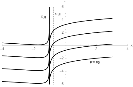
Figure 1: The curves of $\varphi=$ Constant. In this figure, we choose $\epsilon_{c}=1,\;d=1$, $\eta=\sqrt{2}$. The universal horizon (dotted vertical line) is located at $x_{UH}=-1$, and the black vertical line denotes the location of the cosmological Killing horizon located at $x_{KH}=-\frac{1}{\sqrt{2}}$.

From Eq.(IV.2), we can construct a spacelike unit vector $s_{\mu}=s_{0}\delta^{t}_{\mu}+s_{1}\delta^{x}_{\mu}$, which is orthogonal to $u^{\mu}$. It can be shown that $s_{\mu}$ has the non-vanishing components,

$$s_{0} = -(cx+d),$$

$$s_{1} = \frac{\eta xu^{1}-\sqrt{G(x)}}{\eta^{2}x^{2}-1}.$$ (4.26)

Then, we can project $k^{\mu}$ onto $u^{\alpha}$ and $s^{\alpha}$, and obtain,

$$k_{u}\equiv(k\cdot u)=-\omega u^{0}+k_{x}u^{1},$$

$$k_{s}\equiv(k\cdot s)=-\omega u_{1}-k_{x}u_{0}.$$ (4.27)

To proceed further, we need to consider the aether four-velocity $u_{\mu}$ in the regions $x>x_{UH}$ and $x<x_{UH}$, separately. In particular, $\epsilon_{c}$ is set to unity in Eq.(4.22) which leads to the solution,

$$u_{0} = -|d\eta x+\sqrt{d^{2}+1}|,$$

$$u_{1} = d,$$

$$u^{0} = \sqrt{d^{2}+1},$$

$$u^{1} = \eta\sqrt{d^{2}+1}x+d,$$

$$f^{\prime} = -\frac{d}{x\eta d+\sqrt{d^{2}+1}},$$

$$f = -\frac{1}{\eta}\ln\left(\eta xd+\sqrt{d^{2}+1}\right),$$ (4.28)

for $x\textgreater x_{UH}$. When $x\textless x_{UH}$, we find that $u_{0}$ and $u^{1}$ remain the same while $u^{0}$, $u_{1}$, $f^{\prime}$ and $f$ are changed to

$$u^{0} = \frac{\eta^{2}x^{2}\sqrt{d^{2}+1}+2d\eta x+\sqrt{d^{2}+1}}{\eta^{2}x^{2}-1},$$

$$u_{1} = -\frac{2\eta x\sqrt{d^{2}+1}+d\eta^{2}x^{2}+d}{\eta^{2}x^{2}-1},$$

$$f^{\prime} = \frac{d}{x\eta d+\sqrt{d^{2}+1}}+\frac{2\eta x}{1-x^{2}\eta^{2}},$$

$$f = \frac{1}{\eta}\ln\left(\frac{dx\eta+\sqrt{d^{2}+1}}{1-x^{2}\eta^{2}}\right),\;(x\textless x_{UH}).$$ (4.29)

At the universal horizon, similar to the (3+1)-dimensional case DWWZ , relativistic particles cannot be emitted in the form of Hawking radiation. Thus, in the following we consider only the particles with the following non-relativistic dispersion relation DWWZ ,

$$k_{u}^{2}=k_{s}^{2}+a_{2}\frac{k_{s}^{4}}{k_{0}^{2}},$$ (4.30)

where $a_{2}$ is a dimensionless constant of order one, and $k_{0}$ is the cutoff energy scale. For $k\ll k_{0}$, the particles become relativistic. Then, from Eq.(IV.2) we find

$$k_{u} = -\frac{1}{u_{0}}(k_{s}u^{1}-\omega),$$

$$k_{x} = -\frac{1}{u_{0}}(\omega u_{1}+k_{s}).$$ (4.31)

Combined with the dispersion relation (4.30), we find that $k_{s}$ has a simple pole at the universal horizon $x=x_{UH}$ with $u_{0}(x_{UH})=0$. Thus, we assume that near the universal horizon we have

$$k_{s}=-\frac{b(x)}{u_{0}},$$ (4.32)

where $b(x=x_{UH})\neq 0$. To calculate the temperature given by Eq.(4.5) but now at the universal horizon, in principle we only need the Laurent expansion of $k_{x}$ in the neighborhood of the universal horizon. Setting $\epsilon=x-x_{UH}$, for the special case given by Eq.(IV.2), we find

$$u_{0} = -d\eta\epsilon,$$

$$u^{1} = -\frac{1}{d}+\epsilon\eta\sqrt{d^{2}+1},$$

$$b(x) = b_{0}+b_{1}\epsilon+{\cal{O}}\left(\epsilon^{2}\right),$$

$$k_{x} = \frac{b_{0}}{\eta^{2}d^{2}\epsilon^{2}}+\frac{1}{\epsilon}\left(\frac{\rm\omega}{\eta}+\frac{b_{1}}{\eta^{2}d^{2}}\right)+{\cal{O}}\left(1\right),$$ (4.33)

for $x>x_{UH}$, where

$$b_{0} = \pm\frac{k_{0}}{\sqrt{a_{2}}d},$$

$$b_{1} = \eta d^{2}\rm\omega-\eta db_{0}\sqrt{d^{2}+1}.$$ (4.34)

When $x<x_{UH}$, the Taylor expansions of $u^{1}$ and $b(x)$ remain the same as in Eq.(IV.2) while $u_{0}$ and $k_{x}$ are changed to

$$u_{0} = d\eta\epsilon,$$

$$k_{x} = \frac{b_{0}}{\eta^{2}d^{2}\epsilon^{2}}+\frac{1}{\epsilon}\left(-\frac{\rm\omega}{\eta}+\frac{b_{1}}{\eta^{2}d^{2}}\right)+{\cal{O}}\left(1\right),$$ (4.35)

Correspondingly, with the help of dispersion relation Eq.(4.30), one can show

$$b_{0} = \pm\frac{k_{0}}{\sqrt{a_{2}}d},$$

$$b_{1} = -\eta d^{2}\rm\omega-\eta db_{0}\sqrt{d^{2}+1}.$$ (4.36)

In order to figure out the temperature at the universal horizon, one needs to analytically continue the radial momentum $k_{x}$ to the complex plane, combining Eqs.(IV.2) and (IV.2), it’s easy to conclude that, by setting $x=x_{UH}+\epsilon e^{i\theta}$, for $\theta\in(0,2\pi)$

$$k_{x}=\frac{b_{0}}{\eta^{2}d^{2}\epsilon^{2}e^{2i\theta}}+\frac{2\omega}{\eta\epsilon e^{i\theta}}-\frac{b_{0}\sqrt{d^{2}+1}}{\eta d\epsilon},$$ (4.37)

Then, using Eq.(4.5),

$$\frac{\omega}{T_{KH}}=\rm{Im}\oint k^{+}_{x}dx=\frac{4\pi\omega}{\eta},$$ (4.38)

from which we find that,

$$T_{UH}=\frac{\eta}{4\pi}.$$ (4.39)

The surface gravity at the universal horizon is given by Wang17 ,

$$\kappa_{UH}=\frac{1}{2}D_{u}(u\cdot\zeta)=\frac{\eta}{2},$$ (4.40)

from which we find that the standard relation

$$T_{UH}=\frac{\kappa_{UH}}{2\pi},$$ (4.41)

is satisfied at the universal horizon. This is similar to the (3+1)-dimensional case CLMV ; BBMb ; DWWZ . For more general case with the dispersion relation,

$$k_{u}^{2}=k_{s}^{2}\sum_{n=0}^{2z}{a_{n}\left(\frac{k_{s}}{k_{0}}\right)^{n}},$$ (4.42)

it can be shown that the (3+1)-dimensional results DWWZ ,

$$T^{z\geq 2}_{UH}=\frac{\kappa^{z\geq 2}_{UH}}{2\pi}=\left(\frac{2(z-1)}{z}\right)\left(\frac{\kappa_{UH}}{2\pi}\right),$$ (4.43)

can be also obtained.

V Conclusions

In this paper, we studied the non-projectable Hořava gravity coupled with a non-relativistic scalar field, in which the coupling is in general non-minimal through the interaction term $f(\phi)R$. The Hamiltonian structure of this coupled system is very similar to that of pure gravity case. There exist two first-class constraints and two second-class constraints (The combinations of two second-class constraints will generate two global first-class constraints which account for global time reparametrization symmetry of Hořava gravity as first pointed out in DJ ). Therefore, the local degrees of freedom is one due to the presence of the scalar field.

We also found diagonal static solutions for the couplings $f(\phi)=\xi\phi$, and showed that Killing horizons exist in such solutions, but the scalar field turns out to be singular at these Killing horizons. For the non-diagonal stationary solutions, when the lapse function and the spatial metric component $g_{11}$ are set to one, we found that the solutions represent black holes, in which both Killing and universal horizons exist. At the Killing horizon, the temperature of Hawking radiation is proportional to its surface gravity defined as in the relativistic case [cf. Eq.(4.7)] HE73 .

To study locations of the universal horizons, we first considered a test timelike scalar field in such a fixed background LACW , and found solutions of the test field, whereby the universal horizons located at $\chi\cdot u=0$ were found. By using the Hamilton-Jacobi method DWWZ , we calculated the temperature at the universal horizon, and found that it is proportional to the modified surface gravity defined by Eq.(4.40). For $z=2$ of the dispersion relation (4.42), the modified surface gravity given by Eq.(4.40) satisfies the standard relation with its temperature, $T_{UH}={\kappa_{UH}}/({2\pi})$, similar to the (3+1)-dimensional case BBMb ; CLMV . But, in more general cases, both of them will depend on $z$, as shown by Eq.(4.43), although the standard relation, $T^{z\geq 2}_{UH}={\kappa^{z\geq 2}_{UH}}/({2\pi})$, is still expected to hold DL16 ; Cropp16 .

The results presented in this paper show clearly that the existence of universal horizons and their thermodynamics are independent of dimensions of spacetimes concerned. Therefore, the 2d Hořava gravity provides an ideal place to address these important issues, which often technically become very complicated in higher dimensional spacetimes.

References

• (1) S. Carlip, Quantum Gravity in 2+1 Dimensions, Cambridge Monographs on Mathematical Physics (Cambridge University Press, Cambridge, 2003); C. Rovelli, Quantum Gravity, (Cambridge Monographs on Mathematical Physics (Cambridge University Press, Cambridge, 2010); C. Kiefer, Quantum Gravity, third edition (Oxford Science Publications, Oxford University Press, 2012).
• (2) M.B. Green, J.H. Schwarz and E. Witten, Superstring Theory: Vol.1 $\&$ 2, Cambridge Monographs on Mathematical Physics (Cambridge University Press, Cambridge, 1999); J. Polchinski, String Theory, Vol. 1 $\&$ 2 (Cambridge University Press, Cambridge, 2001); K. Becker, M. Becker, and J.H. Schwarz, String Theory and M-Theory (Cambridge University Press, Cambridge, 2007).
• (3) A. Ashtekar and J. Lewandowski, Background independent quantum gravity: A status report, Class. Quantum Grav. 21 (2004) R53 [arXiv:gr-qc/0404018]; M. Bojowald, Canonical Gravity and Applications: Cosmology, Black Holes, and Quantum Gravity (Cambridge University Press, Cambridge, 2011); R. Gambini and J. Pullin, A First Course in Loop Quantum Gravity (Oxford University Press, Oxford, 2011); C. Rovelli and F. Vidotto, Covariant Loop Quantum Gravity: An Elementary Introduction to Quantum Gravity and Spinfoam Theory (Cambridge Monographs on Mathematical Physics, Cambridge, 2015).
• (4) J. Ambjorn, D. Coumbe, J. Gizbert-Studnicki, J. Jurkiewicz, Recent results in CDT quantum gravity, arXiv:1509.08788.
• (5) S. Weinberg, in General Relativity, An Einstein Centenary Survey, edited by S.W. Hawking and W. Israel (Cambridge University Press, Cambridge, 1980); S. Nagy, Lectures on renormalization and asymptotic safety, Ann. Phys. (N.Y.) 350 (2014) 310 [arXiv:1211.4151].
• (6) M. Bojowald, Quantum Cosmology: a review, Rep. Prog. Phys. 78 (2015) 023901 [ arXiv:1501.04899].
• (7) C. Kiefer, and M. Kramer, Can effects of quantum gravity be observed in the cosmic microwave background?, Int. J. Mod. Phys. D21 (2012) 1241001 [arXiv:1205.5161]; L.M. Krauss and F. Wilczek, Using Cosmology to Establish the Quantization of Gravity, Phys. Rev. D89 (2014) 047501 [arXiv:1309.5343]; R.P. Woodard, Perturbative Quantum Gravity Comes of Age, arXiv:1407.4748; A. Ashoorioon, P. S. B. Dev, and A. MazumdarMod, Implications of purely classical gravity for inflationary tensor modes Phys. Lett. A29 (2014) 30; T. Zhu, A. Wang, G. Cleaver, K. Kirsten, Q. Sheng, and Q. Wu, Detecting quantum gravitational effects of loop quantum cosmology in the early universe?, Astrophys. J. Lett. 807 (2015) L17 [arXiv:1503.06761]; Universal features of quantum bounce in loop quantum cosmology, arXiv:1607.06329; T. Zhu, A. Wang, G. Cleaver, K. Kirsten, and Q. Sheng, High-order Primordial Perturbations with Quantum Gravitational Effects, Phys. Rev. D93 (2016) 123525 [arXiv:1604.05739]; D. Baumann and L. McAllister, Inflation and String Theory (Cambridge Monographs on Mathematical Physics, Cambridge University Press, 2015); E. Silverstein, TASI lectures on cosmological observables and string theory, arXiv:1606.03640.
• (8) B. Bolliet, A. Barrau, J. Grain and S. Schander, Observational exclusion of a consistent loop quantum cosmology scenario, Phys. Rev. D93 (2016) 124011; J. Grain, The perturbed universe in the deformed algebra approach of Loop Quantum Cosmology, Inter. J. Mod. Phys. D25 (2016) 1642003 [arXiv:1606.03271].
• (9) K. S. Stelle, Renormalization of higher-derivative quantum gravity, Phys. Rev. D16 (1977) 953.
• (10) M. Ostrogradsky, Mem. Ac. St. Petersbourg, VI4 (1850) 385.
• (11) R. P. Woodard, The Theorem of Ostrogradsky, arXiv:1506.02210.
• (12) P. Hořava, Phys. Rev. D79 (2009) 084008; J. High Energy Phys. 0903, 020 (2009); Phys. Rev. Lett. 102, 161301 (2009).
• (13) D. Anselmi and M. Halat, Renormalization of Lorentz violating theories, Phys. Rev. D76 (2007) 125011 [arXiv:0707.2480]; M. Visser, Lorentz symmetry breaking as a quantum field theory regulator, Phys. Rev. D80 (2009) 025011 [arXiv:0902.0590]; Power-counting renormalizability of generalized Horava gravity, arXiv:0912.4757; T. Fujimori, T. Inami, K. Izumi, and T. Kitamura, Power-counting and Renormalizability in Lifshitz Scalar Theory, Phys. Rev. D91 (2015) 125007 [arXiv:1502.01820]; Tree-Level Unitarity and Renormalizability in Lifshitz Scalar Theory, Prog. Theor. Exp. Phys. 2016 (2016) 013B08 [arXiv:1510.07237].
• (14) H. Lü, J. Mei, and C.N. Pope, Solutions to Horava Gravity, Phys. Rev. Lett. 103 (2009) 091301 [arXiv:0904.1595]; C. Charmousis, G. Niz, A. Padilla, and P.M. Saffin, Strong coupling in Horava gravity, JHEP 0908 (2009) 070 [arXiv:0905.2579]; D. Blas, O. Pujolas, and S. Sibiryakov, On the Extra Mode and Inconsistency of Horava Gravity, JHEP 0910 (2009) 029 [arXiv:0906.3046]; M. Li and Y. Pang, A Trouble with Hořava-Lifshitz Gravity, JHEP 0908 (2009) 015 [arXiv:0905.2751]; M. Henneaux, A. Kleinschmidt and G. Lucena Gómez, A dynamical inconsistency of Hořava gravity, Phys. Rev. D81 (2010) 064002 [arXiv:0912.0399].
• (15) A. Wang, Hořava Gravity at a Lifshitz Point: A Progress Report, Inter. J. Mod. Phys. D26 (2017) 1730014 [arXiv:1701.06087].
• (16) D. Orlando and S. Reffert, On the Renormalizability of Horava-Lifshitz-type Gravities, Class. Quantum Grav. 26 (2009) 155021 [arXiv:0905.0301].
• (17) S. Deser and Z. Yang, Is topologically massive gravity renormalizable? Class. Quantum Grav. 7 (1990) 1603.
• (18) A.O. Barvinsky, D. Blas, M. Herrero-Valea, S.M. Sibiryakov, and C.F. Steinwachs, Renormalization of Horava Gravity, Phys. Rev. D93 (2016) 064022 [arXiv:1512.02250].
• (19) B.-F. Li, A. Wang, Y. Wu, and Z.-C. Wu, Quantization of (1+1)-dimensional Hořava-Lifshitz theory of gravity, Phys. Rev. D90 (2014) 124076 [arXiv:1408.2345].
• (20) B.-F. Li, V. H. Satheeshkumar, and A. Wang, Quantization of 2D Hořava gravity: non-projectable case, Phys. Rev. D93 (2016) 064043 [arXiv:1511.06780].
• (21) R. Jackiw, Lower Dimensional Gravity, Nucl. Phys. B252 (1985) 343.
• (22) J. D. Brown, Lower Dimensional Gravity, (World Scientific Pub. Co. Inc., Singapore 1988).
• (23) D. Grumiller, W. Kummer, and D.V. Vassilevich, Dilaton Gravity in Two Dimensions, Phys. Rept. 369 (2002) 327 [arXiv:hep-th/0204253].
• (24) P.A.M. Dirac, Lectures on quantum mechanics (New York, Belfer Graduate School of Science, Yeshiva University, 1964).
• (25) J. Ambjorn, L. Glaser, Y. Sato, Y. Watabiki, 2d CDT is 2d Horava-Lifshitz quantum gravity, Phys. Lett. B722 (20123) 172 [arXiv:1302.6359].
• (26) J. Ambjorn, A. Gorlich, J. Jurkiewicz, and H.-G. Zhang, A c=1 phase transition in two-dimensional CDT/Horava-Lifshitz gravity? Phys. Lett. B743 (2015) 435 [arXiv:1412.3873].
• (27) H.S. Vieira and V.B. Bezerra, Class of solutions of the Wheeler-DeWitt equation in the Friedmann-Robertson-Walker universe, Phys. Rev. D94 (2016) 023511 [arXiv:1603.02236].
• (28) J.P.M. Pitelli, Quantum Cosmology in (1+1)-dimensional Ho?ava-Lifshitz theory of gravity, Phys. Rev. D93 (2016) 104024 [arXiv:1605.01979].
• (29) S.W. Hawking and G.F.R. Ellis, The large scale structure of space-time, Cambridge Monographs on Mathematical Physics, (Cambridge University Press, Cambridge, 1973).
• (30) D. Blas and S. Sibiryakov, Horava gravity vs. thermodynamics: the black hole case, Phys. Rev. D84, 124043 (2011) [arXiv:1110.2195].
• (31) E. Barausse, T. Jacobson, and T. Sotiriou, Black holes in Einstein-aether and Horava-Lifshitz gravity, Phys. Rev. D83 (2011) 124043 [arXiv:1104.2889].
• (32) K. Lin, O. Goldoni, M. F. da Silva, and A. Wang, New look at black holes: Existence of universal horizons, Phys. Rev. D91 (2015) 024047 [arXiv:1410.6678].
• (33) J. Greenwald, J. Lenells, J.X. Lu, V.H. Satheeshkumar, and A. Wang Black holes and global structures of spherical spacetimes in Horava-Lifshitz theory, Phys. Rev. D84 (2011) 084040 [arXiv:1105.4259].
• (34) P. Berglund, J. Bhattacharyya, and D. Mattingly, Mechanics of universal horizons, Phys. Rev. D85 (2012) 124019 [arXiv:1202.4497].
• (35) B. Cropp, S. Liberati, A. Mohd and M. Visser, Ray tracing Einstein- ther black holes: Universal versus Killing horizons, Phys. Rev. D89 (2014) 064061 [arXiv:1312.0405].
• (36) C. Ding, A. Wang and X. Wang, Charged Einstein-aether black holes and Smarr formula, Phys. Rev. D92 (2015) 084055 [arXiv:1507.06618].
• (37) P. Berglund, J. Bhattacharyya, and D. Mattingly, Towards Thermodynamics of Universal Horizons in Einstein-Eather Theory Phys. Rev. Lett. 110 (2013) 071301 [arXiv:1210.4940].
• (38) C. Ding, A. Wang, X. Wang and T. Zhu, Hawking radiation of charged Einstein-aether black holes at both Killing and universal horizons, Nucl. Phys. B913 (2016) 694 [arXiv:1512.01900].
• (39) C.-K. Ding and C.-Q. Liu, Dispersion relation and surface gravity of universal horizons, arXiv:1611.03153.
• (40) B. Cropp, Strange Horizons: Understanding Causal Barriers Beyond General Relativity, arXiv:1611.00208.
• (41) D. Bazeia, F.A. Brito, and F.G. Costa, Two-dimensional Horava-Lifshitz black hole solutions, Phys. Rev. D91 (2015) 044026 [arXiv:1409.0490].
• (42) K. Lin, E. Abdalla, R.-G. Cai, and A. Wang, Inter. J. Mod. Phys. D23, 1443004 (2014).
• (43) T. Jacobson and D. Mattingly, Phys. Rev. D63, 041502 (2001); T. Jacobson, Proc. Sci. QG-PH, 020 (2007).
• (44) R. Arnowitt, S. Deser, and C.W. Misner, Gen. Relativ. Gravit. 40, 1997 (2008); C.W. Misner, K.S. Thorne, and J.A. Wheeler, Gravitation (W.H. Freeman and Company, San Francisco, 1973), pp.484-528.
• (45) C. Eling and T. Jacobson, Phys. Rev. D74, 084027 (2006).
• (46) W. Donnelly and T. Jacobson, Phys. Rev. D84, 104019 (2011).
• (47) T. Jacobson, Phys. Rev. D89, 081501 (2014).