x-ray insights into the nature of quasars with redshifted broad absorption lines

Abstract

We present Chandra observations of seven broad absorption line (BAL) quasars at $z=0.863$–2.516 with redshifted BAL troughs (RSBALs). Five of our seven targets were detected by Chandra in 4–13 ks exposures with ACIS-S. The $\alpha_{\rm ox}$ values, $\Delta\alpha_{\rm ox}$ values, and spectral energy distributions of our targets demonstrate they are all X-ray weak relative to expectations for non-BAL quasars, and the degree of X-ray weakness is consistent with that of appropriately-matched BAL quasars generally. Furthermore, our five detected targets show evidence for hard X-ray spectral shapes with a stacked effective power-law photon index of $\Gamma_{\rm eff}=0.5^{+0.5}_{-0.4}$. These findings support the presence of heavy X-ray absorption ($N_{\rm H}\approx 2\times 10^{23}$ cm^-2) in RSBAL quasars, likely by the shielding gas found to be common in BAL quasars more generally. We use these X-ray measurements to assess models for the nature of RSBAL quasars, finding that a rotationally-dominated outflow model is favored while an infall model also remains plausible with some stipulations. The X-ray data disfavor a binary quasar model for RSBAL quasars in general.

1. INTRODUCTION

Broad Absorption Lines (BALs) are observed in $\approx 15$% of optically selected quasars within the redshift range of $1.5\leq z\leq 2.5$ (e.g., Hewett & Foltz, 2003; Gibson et al., 2009), defined by requiring the velocity width of the BAL absorption trough to be above 2000 km s^-1 (e.g., Weymann et al., 1991). The intrinsic fraction of BAL quasars, after correcting for observational selection effects, is even higher (e.g., Hewett & Foltz, 2003; Dai et al., 2008; Allen et al., 2011). The BAL troughs are almost always blueshifted relative to the corresponding emission lines in rest-frame ultraviolet (UV) spectra, implying the presence of fast outflowing winds. BAL troughs can extend to velocities of at least $\approx 60000$ km s^-1 (e.g., Rogerson et al., 2016). Outflowing quasar winds appear to be a key for understanding how supermassive black holes (SMBHs) may be agents of feedback to typical massive galaxies (e.g., Chartas et al., 2009; Fabian, 2012; Arav et al., 2013; King, 2014).

BAL quasars are commonly classified into one of three groups based on the ionization levels of the observed BALs. High-ionization BAL quasars (HiBALs) only contain high-ionization BALs such as C IV, N V, and O VI. Low-ionization BAL quasars (LoBALs) show, in addition to the high-ionization BALs, low-ionization BALs such as C II, Al III, and Mg II. Iron low-ionization BAL quasars (FeLoBALs) are LoBALs that also possess BALs from Fe II and/or Fe III.

BAL quasars usually have low soft X-ray fluxes compared to their optical/UV fluxes (e.g., Green & Mathur, 1996; Gallagher et al., 2006), and X-ray spectroscopy reveals that this behavior is often due to heavy and complex X-ray absorption of a nominal-strength underlying X-ray continuum (e.g., Gallagher et al., 2002, 2006; Fan et al., 2009). Thus, the level of X-ray continuum luminosity, evaluated using observed $\alpha_{\rm ox}$ and $\Delta\alpha_{\rm ox}$, is significantly different between BAL quasars and non-BAL quasars. Here $\alpha_{\rm ox}$ is defined as $0.3838\log(l_{\rm 2~{}keV}/l_{2500~{}\mathring{\rm{A}}})$, indicating the relationship between rest-frame X-ray (2 keV) and UV (2500 Å) luminosity. The quantity $\Delta\alpha_{\rm ox}$ is $\alpha_{\rm ox}({\rm Observed})-\alpha_{\rm ox}(l_{2500~{}\mathring{\rm{A}}})$, representing the observed $\alpha_{\rm ox}$ relative to that expected from the established $\alpha_{\rm ox}$-$l_{2500~{}\mathring{\rm{A}}}$ relation (e.g., Steffen et al., 2006).

Murray et al. (1995) proposed an influential accretion-disk wind model for BAL quasars, where an equatorial wind is launched from the disk at $\approx 10^{16}$–$10^{17}$ cm from the central SMBH ($\approx 10^{8}$–$10^{9}M_{\odot}$) and radiatively driven by UV-line pressure. To accelerate the observed gas to a high velocity efficiently, this model invokes a “failed wind” as shielding gas to prevent nuclear X-ray and extreme-UV (EUV) photons from over-ionizing the outflowing gas observed in the UV (e.g., Proga et al., 2000); X-ray absorption by such shielding gas can explain the observed X-ray weakness of many BAL quasars. While this model has had many successes, it also faces some challenges. For example, it has been argued that the observed level of X-ray shielding is insufficient to protect the wind from over-ionization, and that gas clumping may instead be responsible for maintaining the needed ionization level (e.g., Hamann et al., 2013; Baskin et al., 2014). Additionally, at least some absorbers are thought to be located at kpc-scale distances from the SMBH, leading to alternative suggestions about acceleration mechanisms (e.g., Arav et al., 2013; Borguet et al., 2013).

While, as noted above, almost all BALs are blueshifted relative to the corresponding emission lines, rare quasars with redshifted BALs (RSBALs) have now been identified in significant numbers. Some of these objects have both redshifted and blueshifted BALs, while others contain only RSBALs. In the large quasar spectroscopic databases of the Sloan Digital Sky Survey-I/II/III (SDSS-I/II/III; e.g., York et al., 2000; Eisenstein et al., 2011), Hall et al. (2013) found 17 BAL quasars with RSBALs in C IV and two with Mg II RSBALs. In this sample of quasars with RSBALs, the velocity widths of the RSBALs are above 3000 km s^-1, except for one case, and the RSBALs can extend to redshifted velocities up to about 15000 km s^-1. All of the three BAL-quasar ionization classes (HiBALs, LoBALs, and FeLoBALs) are found for quasars with RSBALs. Notably, the fraction of LoBAL quasars in the RSBAL quasar sample is much higher than that in the general population of BAL quasars; this result may be a clue to the nature of quasars with RSBALs. Among BAL quasars, the objects with RSBALs may provide novel broader insights about quasar inflows/outflows, and they may represent a new method for observing the fueling/feedback of SMBHs.

Hall et al. (2013) proposed three models that might explain the nature of quasars with RSBALs: a rotationally-dominated outflow model, an infall model, and a binary quasar model. These are briefly described below:

1. The rotationally-dominated outflow model predicts that redshifted absorption can arise when the accretion disk, an extended emission source, is seen through a rotating outflow launched from the disk. This scenario proposes that, at some locations, the outflow has a rotational velocity that dominates the component along our line of sight of its poloidal outflow velocity (e.g., see Figure 1 and Ganguly et al., 2001; Hall et al., 2002). Such a scenario can most likely occur when the accretion disk is viewed at high inclination. This model can naturally explain the presence of both redshifted and blueshifted absorption when both are present, and it can also produce only redshifted absorption if the outflow is azimuthally asymmetric (so that outflowing material is only present in regions where the rotational velocity dominates over the component along our line of sight of the poloidal outflow velocity).

   Figure 1.— Line-of-sight velocity field of the near side of a rotating, accelerating disk wind, seen at inclination $i=89\arcdeg$ in the top panel and as labelled in the other panels. The central black dot shows the black hole’s location. We see the wind from only one side of the optically thick accretion disk, and only the velocities from the near side of the funnel-shaped wind are plotted. The black ellipse shows the continuum emission region of the disk, against which the wind is silhouetted; the wind is launched from a narrow annulus just outside that region. Absorption would only be seen at the velocities found within the black ellipse. The ratio of redshifted to blueshifted absorption decreases with decreasing inclination angle. Different choices for the initial velocity, terminal velocity, acceleration profile, or launching radius of the wind would change its velocity field in detail but not qualitatively.

2. The infall model proposes that we are observing, via RSBALs, material infalling toward the SMBH along the line of sight. To generate redshifted absorption extending to the high velocities often observed, infall down to a few hundred Schwarzschild radii is required. A challenge for this model is that such infalling gas is generally expected to have higher ionization levels than observed (e.g., Proga & Kallman, 2004). However, infall and disruption of dense and initially opaque clumps, for which a quasar’s radiation pressure cannot overcome the pull of the SMBH’s gravity, might allow gas to reach the small required radii while maintaining a low ionization state.

3. The binary quasar model proposes that RSBALs are found in binary quasar systems with separations of hundreds of pc to a few kpc (the kpc-scale upper limit is imposed by current optical-imaging constraints). In this model, an outflow from the closer, fainter member of the binary is backlit by the more distant, brighter member (e.g., Civano et al., 2010; Hall et al., 2013). Hall et al. (2013) argued against the general applicability of the binary model, since basic estimates of the number of suitable binaries appeared too small compared with the observed number of quasars with RSBALs. However, further considerations of the timing of the quasar phase in merger models, sample-selection effects, and the final-pc problem indicate that binary quasars may indeed be sufficiently common that they could plausibly explain all quasars with RSBALs (E.S. Phinney and P.F. Hopkins 2013, private communication).

In this paper, we analyze and interpret exploratory Chandra X-ray observations of a sample of seven quasars with RSBALs. The observed targets were chosen from the catalog of Hall et al. (2013) to have RSBALs in either C IV or Mg II. All targets were selected to have bright optical fluxes, allowing sufficiently sensitive Chandra observations to be obtained economically. We also favored targeting objects with no or relatively weak (compared to the RSBAL strength) blueshifted BALs; this should help in isolating effects due to RSBALs from those due to blueshifted BALs. Aside from defining the basic X-ray properties of quasars with RSBALs for the first time, we also would like to utilize X-ray emission to clarify which of the three models above best explains the nature of RSBALs. For example, X-ray absorbing shielding gas along the line of sight is expected for the rotationally-dominated outflow model, since this model adopts the essentials of the standard accretion-disk wind scenario for BAL quasars. In contrast, X-ray absorption is not expected for the binary quasar model since, in this model, the background quasar producing most of the observed X-ray emission is not launching the wind that creates the RSBALs. For the infall model, X-ray absorption along the line of sight is not automatically expected but is perhaps possible.

We describe our sample selection, the utilized Chandra observations, and the X-ray data analysis in Section 2. To examine the physical characteristics of our sample, we present multiwavelength (radio, infrared, optical, and UV) data as well as the X-ray weakness parameter in Section 3. In Section 4, we discuss three possible explanations for the RSBAL quasars in light of our X-ray results. Our results are summarized in Section 5 where we also discuss future prospects. We adopt the cosmological parameters $H_{0}=67.8$ km s^-1 Mpc^-1, $\Omega_{\rm M}=0.308$, and $\Omega_{\Lambda}=0.692$ throughout the paper (Planck Collaboration et al., 2015).

2. Sample Selection, Sample Properties, and CHANDRA Analysis

2.1. Sample Selection and Properties

The redshift and absolute $i$-band magnitude of our targeted RSBAL quasar sample compared to the RSBAL quasars in Hall et al. (2013) are shown in Figure 2. Various properties of our targets are summarized in Table 1. The RSBAL quasars we targeted with Chandra have redshifts of 0.863–2.516. All seven objects in our X-ray sample were selected from a sample of RSBAL quasars in Hall et al. (2013). Among five targeted quasars with redshifted C IV BALs, we prioritized those with strong redshifted absorption and weak or absent blueshifted absorption (J0830+1654, J1724+3135, and J2157$-$0022); this should isolate effects due to redshifted vs. blueshifted absorption. For example, the C IV trough in J2157$-$0022 shows a sharp edge at small blueshifted velocities (1930 km s^-1) and smoothly extends to large redshifted velocities of 9050 km s^-1. In addition, two lower redshift objects, J1125+0029 and J1128+0113 from Hall et al. (2013), were selected based on confirmed Mg II redshifted absorption. Our targets were chosen to have bright optical fluxes, with $i$-band apparent magnitudes of 17.9–20.1, in order to enable suitably sensitive Chandra observation to be obtained efficiently. To avoid any complicating effects associated with jet-linked X-ray emission (e.g., Miller et al., 2011), we required all targets to be radio quiet with radio-loudness parameters of $R<10$, where $R=f_{5~{}{\rm GHz}}/f_{\rm 4400~{}{\textup{\AA}}}$ (Kellermann et al., 1989).

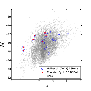
Figure 2.— The red stars indicate the redshift and SDSS absolute $i$-band magnitude of the seven RSBALs in our sample. The blue circles show the confirmed RSBALs from Hall et al. (2013). For comparision, the gray dots represent the 29580 BAL quasars from the SDSS DR12 quasar catalog. The vertical dashed line ($z=1.5$) marks the minimum redshift where the spectra of our sample objects start to have C IV coverage. The quasars J1125+0029 and J1128+0113 are the two RSBALs that lack C IV coverage in their observations.

Three BAL groups are included in our sample (see Table 1). Six of our targets are LoBALs, as low-ionization absorption is common among RSBALs. Two of these six are FeLoBALs. Only one of our targets is a HiBAL.

Four of our RSBAL quasars have two epochs of SDSS observations, and all four show variability of their redshifted C IV or Mg II absorption (Hall et al., 2013). Three quasars (J1034+0720, J1628+4744, and J1128+0112 ) only show significant variability of their RSBALs, while J1125+0029 shows variability of both its redshifted and blueshifted BALs.

Table 1RSBAL Quasar Properties

Object Name	Redshift	BAL	C IV	C IV	C IV	$M_{i}$	$N_{\rm H,Gal}$	$E(B-V)$
		type	AItot	AI-	AI+
(J2000)			(km s-1)	(km s-1)	(km s-1)		($10^{20}$cm-2)
(1)	(2)	(3)	(4)	(5)	(6)	(7)	(8)	(9)
$083030.26+165444.7$	$2.435$	Lo	2069$\pm$175	743$\pm$72	1326$\pm$102	$-27.17$	$3.8$	0.03
$103412.33+072003.6$	$1.689$	Lo	2116$\pm$22	2035$\pm$7	81$\pm$28	$-26.85$	$2.9$	0.03
$112526.12+002901.3$	$0.863$	FeLo	…	…	…	$-25.54$	$3.7$	0.03
$112828.31+011337.9$	$0.893$	FeLo	…	…	…	$-25.16$	$3.3$	0.03
$162805.80+474415.6$	$1.595$	Hi	3225$\pm$422	2058$\pm$141	1167$\pm$282	$-26.38$	$1.4$	0.02
$172404.44+313539.6$	$2.516$	Lo	3812$\pm$618	0	3812$\pm$618	$-26.86$	$3.3$	0.04
$215704.26-002217.7$	$2.240$	Lo	3956$\pm$221	1329$\pm$34	2627$\pm$187	$-26.18$	$5.4$	0.09

Note. — Cols. (1)–(3): Object name, redshift, and BAL type from Table 1 of Hall et al. (2013). Cols. (4)–(6): The absorption index in km s^-1 for C IV absorption at all velocities (AI^tot), C IV blueshifted absorption (AI^-), and C IV redshifted absorption (AI⁺) from Table 2 of Hall et al. (2013). Two optical spectroscopic observations were available for J1034+0720 and J1628+4744; we selected the one with lower uncertainties. An entry of “…” indicates that C IV is not covered in the optical spectra. Col. (7): Absolute $i$-band magnitude. Col. (8): Galactic neutral hydrogen column density in units of $10^{20}$cm^-2, computed using COLDEN. Col. (9): The standard Galactic extinction $E(B-V)$ values derived from SDSS extinction values.

2.2. Chandra Observations

Our Chandra observations of RSBAL quasars were performed between 2014 Dec 28 and 2016 April 22 using the Advanced CCD Imaging Spectrometer (ACIS; Garmire et al., 2003) spectroscopic array (ACIS-S). The details of the Chandra observations are summarized in Table 2. The targets were placed on the S3 CCD, as is standard. We used VFAINT mode to allow optimal background removal. The targets have exposure times of 3.8–13.1 ks. These exposures were set to obtain detections even if our targets are 6–20 times X-ray weaker than typical quasars, given their optical/UV luminosities (e.g., Steffen et al., 2006). This sensitivity level was required given that BAL quasars are commonly X-ray weak and/or absorbed (e.g., Gallagher et al., 2002, 2006; Luo et al., 2014).

2.3. X-ray Data Analysis

We processed the X-ray data using Chandra Interactive Analysis of Observations (CIAO) tools. For the data set of each source, we applied the chandra_repro script with VFAINT background cleaning. Background flares were removed with the deflare script using sigma clipping at the $3\sigma$ level (little background flaring was present). The final exposure times are listed in Table 2.

To identify our targets, we first ran the wavdetect script on the soft-band (0.5–2.0 keV), hard-band (2.0–8.0 keV), and full-band (0.5–8.0 keV) images using the standard wavelet scales (i.e., 1.0, 1.414, 2.0, 2.828, and 4.0 pixels) and a false-positive probability threshold of $10^{-5}$. Five of the seven targets are detected in at least one band within 1.5″ of their SDSS positions; the two sources not detected by this procedure are J0830+1654 and J1128+0113. Next, aperture photometry was performed for each target by extracting counts from a circular aperture of radius 1.5″; this aperture size provides a suitable balance between capturing source counts and minimizing background counts. Background was extracted from an annular region with inner radius 10″ and outer radius 40″; background point sources in this annulus were removed when measuring the background counts. We assessed the significance of the source signal by computing a binomial no-source probability, $P_{B}$ (e.g., Broos et al., 2007; Xue et al., 2011; Luo et al., 2013, 2015). The definition of $P_{B}$ is

$$P_{B}=\sum^{N}_{X=S}\frac{N!}{X!(N-X)!}p^{X}(1-p)^{N-X}.$$

In this equation, $S$ is the number of source counts; $N$ is the combined number of source and background counts; and $p=1$/(1+BACKSCALE), where BACKSCALE is the ratio of the areas between the background and the source. In agreement with the results from wavdetect, five of the seven targets were detected in at least one band with a $P_{B}$ value lower than 0.01 (i.e., a probability of detection above 99%); the sources not detected were again J0830+1654 and J1128+0113. The source counts were corrected using the enclosed-counts fractions of the Chandra point spread function (PSF) of 0.951, 0.892, and 0.922 for the soft, hard, and full bands, respectively. The net counts for each band, computed from the source and background counts, are listed in Table 2 (with $1\sigma$ uncertainties). For bands where a source is not detected, a 90% confidence-level upper limit is given on the counts following Kraft et al. (1991).

Table 2New Chandra Observations and X-ray Photometric Properties of RSBAL quasars

Object Name	Observation	Observation	Exposure	Counts	Counts	Counts	Hardness	$\Gamma_{\rm eff}$	$N_{\textrm{H}}$
	ID	Start Date	Time	(0.5–2 keV)	(2–8 keV)	(0.5–8 keV)	Ratio
(J2000)		(UT)	(ks)						($10^{23}$cm-2)
(1)	(2)	(3)	(4)	(5)	(6)	(7)	(8)	(9)	(10)
$083030.26+165444.7$	$17043$	2015-05-09	$5.8$	$<2.4$	$<2.6$	$<2.5$	…	…	…
$103412.33+072003.6$	$17045$	2015-06-29	$4.1$	$<2.4$	$2.2_{-1.4}^{+2.7}$	$2.1_{-1.4}^{+2.7}$	$>1.19$	$<0.8$	$>1.3$
$112526.12+002901.3$	$17042$	2015-07-03	$3.8$	$<2.4$	$2.2_{-1.4}^{+2.7}$	$2.1_{-1.4}^{+2.7}$	$>1.19$	$<0.8$	$>0.5$
$112828.31+011337.9$	$17046$	2016-04-22	$5.4$	$<2.4$	$<2.6$	$<2.5$	…	…	…
$162805.80+474415.6$	$17044$	2015-08-05	$4.9$	$2.1_{-1.3}^{+2.7}$	$<2.6$	$2.1_{-1.4}^{+2.7}$	$<1.0$	$>0.9$	$<0.9$
$172404.44+313539.6$	$17040$	2015-11-15	$9.9$	$2.1_{-1.3}^{+2.7}$	$3.3_{-1.7}^{+3.0}$	$5.3^{+3.5}_{-2.3}$	$1.54^{+2.12}_{-0.93}$	$0.5^{+0.9}_{-0.8}$	$4.3^{+5.0}_{-3.3}$
$215704.26-002217.7$	$17041$	2014-12-28	$13.1$	$5.2_{-2.2}^{+3.5}$	$6.6_{-2.5}^{+3.7}$	$11.8^{+4.6}_{-3.4}$	$1.28^{+0.95}_{-0.59}$	$0.7^{+0.6}_{-0.5}$	$2.6^{+2.1}_{-1.6}$

Note. — Cols. (1)–(4): Object name, Chandra observation ID, observation start date, and background-flare cleaned effective exposure time. Cols. (5)–(7): Aperture-corrected net counts in the soft (0.5–2 keV), hard (2–8 keV), and full (0.5–8 keV) observed-frame bands. An upper limit at a 90% confidence level is given if the source is not detected. Col. (8): Hardness ratio between the hard-band and soft-band counts within a 68% confidence interval calculated using the BEHR approach. An entry of “…” indicates that the source is undetected in both bands. Col. (9): 0.5–8 keV effective power-law photon index, derived from the hardness ratio assuming a power-law spectrum modified by Galactic absorption. An entry of “…” indicates that the index cannot be constrained. Col. (10): The estimated intrinsic neutral hydrogen column densities, derived from the hardness ratios assuming a standard X-ray power-law spectrum with a photon index of 2.0 (see §4.1 for further discussion of these quantities).

A hardness ratio between hard-band and soft-band counts, along with its $1\sigma$ error bar, was computed using the Bayesian Estimation of Hardness Ratios (BEHR) approach of Park et al. (2006) due to the failure of standard error propagation for X-ray sources with small numbers of counts (see Table 2). An effective power-law photon index, $\Gamma_{\rm eff}$, was derived from the hardness ratio of each source using the Portable, Interactive, Multi-Mission Simulator (PIMMS) assuming a power-law spectrum modified by Galactic absorption; as expected from the limited numbers of counts, these $\Gamma_{\rm eff}$ values for individual sources have significant uncertainties. Applying stacking of the source counts, we also derived a stacked $\Gamma_{\rm eff}$ for the five detected targets of $0.5^{+0.5}_{-0.4}$ and a stacked $\Gamma_{\rm eff}$ for the four detected LoBAL targets of $0.3^{+0.5}_{-0.4}$. We estimate the full-band X-ray fluxes of our targets from their full-band count rates with PIMMSv4.8d using a power-law spectrum and $\Gamma_{\rm eff}$ (see Table 2). When a source had a lower or upper limit for $\Gamma_{\rm eff}$, we used the limit value in this flux calculation. Furthermore, based on our stacking results, we adopted $\Gamma_{\rm eff}=0.3$ for our two X-ray undetected LoBAL quasars, J0830+1654 and J1128+0113, when deriving upper limits on their full-band fluxes. Our derived flux values are not strongly sensitive to the adopted $\Gamma_{\rm eff}$. The rest-frame 2–10 keV luminosities of our RSBAL quasars were computed from their full-band fluxes with the standard bandpass correction for redshift.

3. Multiwavelength Analysis

3.1. The X-ray-to-Optical Power-Law Slope

We list the X-ray-to-optical power-law slopes (i.e., $\alpha_{\rm ox}$ values) for our sample in Table 3. The observed flux densities at rest-frame 2500 Å for those RSBAL quasars (J1034+0720, J1125+0029, J1128+0113, and J1628+4744) having SDSS spectroscopic observations were estimated by normalizing a power-law model with a fixed spectral index of $-0.5$. To avoid strong absorption and emission lines, the initial fitting regions were chosen based on the spectral windows described in Gibson et al. (2009). For those targets (J0830+1654, J1724+3135, and J2157$-$0022) with only BOSS observations, we calculated their flux densities at rest-frame 2500 Å from the $i$-band apparent PSF magnitudes in the SDSS DR12 quasar catalog (Pâris et al., 2017) with a K-correction and a Galactic-absorption correction. The rest-frame 2 keV flux densities were calculated from the Galactic absorption-corrected full-band fluxes assuming a power-law spectrum with a photon index of $\Gamma_{\rm eff}$ (see §2.3 for further details). The X-ray weakness parameter, $f_{\rm weak}$, listed in Table 3 was derived from $\Delta\alpha_{\rm ox}$ as $f_{\rm weak}=403^{-\Delta\alpha_{\mbox{\tiny OX}}}$, and it represents the factor by which a quasar is X-ray weak relative to the average non-BAL quasar.

Table 3X-ray and Optical Photometric and SED Properties

Object Name	Count Rate	$F_{\rm 0.5-8keV}$	$f_{\rm 2~{}keV}$	$f_{\rm 2500~{}\textup{\AA}}$	$\log L_{\rm X}$	$\log$ $l_{\mbox{\scriptsize 2500 \AA}}$	$\alpha_{\rm OX}$	$\Delta\alpha_{\rm OX}(\sigma)$	$f_{\rm weak}$	$R$
(J2000)	(0.5–8 keV)	($10^{-14}$)	($10^{-33}$)	($10^{-27}$)	(2–10 keV)
	($10^{-3}$ s-1)	(erg cm-2 s-1)	(erg cm-2 s-1Hz-1)		(erg s-1)	(erg s-1Hz-1)
(1)	(2)	(3)	(4)	(5)	(6)	(7)	(8)	(9)	(10)	(11)
$083030.26+165444.7$	$<0.43$	$<0.84$	$<1.2$	$0.90$	$<43.84$	$31.11$	$<-2.26$	$<-0.61(3.58)$	$>37.8$	$<6.3$
$103412.33+072003.6$	$0.53^{+0.67}_{-0.33}$	$0.79$	$3.2$	$1.67$	$43.75$	$31.10$	$-2.20$	$-0.55(3.23)$	$26.8$	$<2.6$
$112526.12+002901.3$	$0.57^{+0.72}_{-0.36}$	$0.85$	$3.7$	$1.47$	$43.25$	$30.48$	$-2.15$	$-0.59(3.00)$	$34.1$	$<2.2$
$112828.31+011337.9$	$<0.46$	$<0.89$	$<1.9$	$1.02$	$<43.24$	$30.35$	$<-2.20$	$<-0.65(3.42)$	$>50.4$	$<3.1$
$162805.80+474415.6$	$0.44^{+0.56}_{-0.28}$	$0.61$	$2.9$	$1.13$	$43.62$	$30.88$	$-2.15$	$-0.53(2.93)$	$23.8$	$<4.1$
$172404.44+313539.6$	$0.54^{+0.35}_{-0.23}$	$0.95$	$2.0$	$0.62$	$43.99$	$30.97$	$-2.11$	$-0.48(2.71)$	$17.4$	$<8.4$
$215704.26-002217.7$	$0.90^{+0.35}_{-0.26}$	$1.44$	$4.6$	$0.42$	$44.18$	$30.72$	$-1.90$	$-0.31(1.63)$	$6.3$	$<10.0$

Note. — Col. (1): Object name. Col. (2): Observed 0.5–8 keV Chandra count rate in units of 10^-3 s^-1. Col. (3): Galactic absorption-corrected observed-frame 0.5–8 keV flux in units of $10^{-14}$ erg cm^-2 s^-1, computed using the PIMMSv4.8d with the power-law photon index in Table 2. When the power-law photon index is an upper or lower limit, we use the limit value for our calculation. We adopt $\Gamma=0.3$ for two undetected targets J0830+1654 and J1128+0113 (see §2.3 for details). Col. (4): Observed flux density at rest-frame 2 keV in units of $10^{-33}$ erg cm^-2 s^-1 Hz^-1, calculated from the unabsorbed 0.5–8 keV flux in the observed frame. Col. (5): Observed flux density at rest-frame 2500 Å in units of $10^{-27}$ erg cm^-2 s^-1 Hz^-1. Optical SDSS spectroscopic observations were available for J1034+0720, J1125+0029, J1128+0113, and J1628+4744. Based on fitting a power-law model with a fixed spectral index of $-0.5$, we calculated the flux density at rest-frame 2500 Å for each of these SDSS observations. The flux densities of targets (J0803+1654, J1724+3135, and J2157-0022) with only BOSS observations were extrapolated from the SDSS $i$-band apparent PSF magnitudes (see §3.1 for details). Col. (6): Logarithm of the rest-frame 2–10 keV luminosity in units of erg s^-1, derived from the observed 0.5–8 keV flux. Col. (7): Logarithm of the rest-frame 2500 Å monochromatic luminosity in units of erg s^-1 Hz^-1. Col. (8): Measured $\alpha_{\rm OX}$ parameter. Col. (9): Difference between the measured $\alpha_{\rm OX}$ and the expected $\alpha_{\rm OX}$ from the Just et al. (2007) $\alpha_{\rm OX}$–$l_{\mbox{\scriptsize 2500 \AA}}$ relation. The statistical significance of this difference, measured in units of the $\alpha_{\rm OX}$ rms scatter in Table 5 of Steffen et al. (2006), is given in the parentheses. Col. (10): Factor of X-ray weakness in accordance with $\Delta\alpha_{\rm OX}$. Col. (11): Radio-loudness parameter, defined as $R=f_{5~{}{\rm GHz}}/f_{\rm 4400~{}{\textup{\AA}}}$, where $f_{5~{}{\rm GHz}}$ and $f_{\rm 4400~{}{\textup{\AA}}}$ are the flux densities at rest-frame 5 GHz and 4400 Å, respectively.

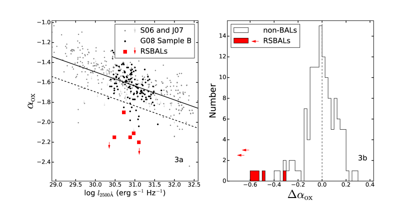
Figure 3.— Left panel: X-ray-to-optical power-law slope ($\alpha_{\rm ox}$) vs. monochromatic luminosity at rest-frame 2500 ${\rm\AA}$ ($l_{\mbox{\scriptsize 2500 \AA}}$) for our RSBAL sample (red squares). The RSBAL sample of seven targets was observed by Chandra and two upper limits (represented by arrows) are shown for J0830+1654 and J1128+0113. Other samples in the figure are non-BALs from G08 sample B (improved following Wu et al., 2011), shown as black dots, and a combination of AGN samples from S06 and J07 is indicated by gray dots and downward arrows. The solid line represents the best-fit relation between $\alpha_{\rm ox}$ and $l_{\mbox{\scriptsize 2500 \AA}}$ from Just et al. (2007); the dashed line ($\Delta\alpha_{\rm ox}=-0.2$) separates X-ray normal and X-ray weak quasars. All seven of our targets are located in the X-ray weak region. Right panel: distribution of $\Delta\alpha_{\rm ox}$ for our RSBAL sample (shaded histograms) compared with the 132 non-BALs from G08 sample B. The two leftward red arrows are the upper limits of J0830+1654 and J1128+0113. The vertical dashed line indicates $\Delta\alpha_{\rm ox}=0$. All of our targets are in the X-ray-weak wing of the distribution, with six being significantly X-ray weaker than any of the G08 Sample B quasars.

Figure 3a displays $\alpha_{\rm ox}$ vs. $l_{\mbox{\scriptsize 2500 \AA}}$ for RSBAL quasars. We also show, for comparison purposes, non-BAL quasars from Gibson et al. (2008; G08) sample B (improved following footnote 16 of Wu et al., 2011) and a combination of AGNs from Steffen et al. (2006; S06) and Just et al. (2007; J07). The solid line represents the best-fit relationship between $\alpha_{\rm ox}$ and $l_{\mbox{\scriptsize 2500 \AA}}$ from Steffen et al. (2006). Following Luo et al. (2015), we adopt $\Delta\alpha_{\rm ox}=-0.2$ (the dashed line in Figure 3a) as a reasonable division between X-ray weak and X-ray normal quasars. All of our targets are located in the X-ray weak region. In addition, in Figure 3b we compare the $\Delta\alpha_{\rm ox}$ distribution of our sample with that for non-BAL quasars from the improved sample B of G08. We adopt the log-rank test (e.g., Feigelson & Babu, 2012) to assess if our censored RSBAL sample follows the same distribution as the non-BAL sample. As clearly expected from the visual appearance, the resulting $p$-value of 0 demonstrates a significant difference between the $\Delta\alpha_{\rm ox}$ values of RSBAL quasars and non-BAL quasars.

We have also compared the $\Delta\alpha_{\rm ox}$ values of our RSBAL quasars to those for LoBAL and HiBAL quasars using the samples from Gibson et al. (G09; 2009) (see Figure 4). Comparing the $\Delta\alpha_{\rm ox}$ values of our low-ionization RSBAL quasars with those for LoBAL quasars from G09, we find they appear consistent; the $p$-value of 0.4 from the log-rank test indicates no statistically significant difference. Furthermore, our low-ionization RSBAL quasar sample does show a significant difference from the HiBAL quasar sample of G09 ($p$-value $\approx 2\times 10^{-5}$). This result demonstrates that the $\Delta\alpha_{\rm ox}$ values of low-ionization RSBAL quasars resemble those of typical LoBAL quasars more than those of typical HiBAL quasars. While we have only one high-ionization RSBAL quasar, its $\Delta\alpha_{\rm ox}$ value also appears consistent with those of HiBAL quasars from G09.

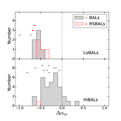
Figure 4.— Distribution of $\Delta\alpha_{\rm ox}$ for our RSBAL sample compared with LoBALs (upper panel) and HiBALs (lower panel) from the samples of G09. The two red leftward arrows represent upper limits for J0830+1654 and J1128+0113. The gray leftward arrows show upper limits for BAL quasars from the samples of G09. The vertical dashed line indicates $\Delta\alpha_{\rm ox}=0$. The upper panel shows the LoBAL quasars in our RSBAL sample resemble those of typical LoBAL quasars. In the lower panel, although we only have one HiBAL quasar in our RSBAL sample, its $\Delta\alpha_{\rm ox}$value is consistent with those HiBAL quasars from the samples of G09.

The $\alpha_{\rm ox}$ and $\Delta\alpha_{\rm ox}$ values of our RSBAL quasars do not seem to depend obviously upon the relative strengths of the redshifted vs. blueshifted UV absorption, although the sample size is too small for tight constraints in this respect.

Although reddening is commonly observed in the spectra of BAL quasars and especially in LoBAL quasars (e.g., Trump et al., 2006; Gibson et al., 2009), none of the SDSS spectra of our Chandra targets shows strong reddening such as exhibited by J0941$-$0229 and J1147$-$0250 in figures 2 and 4, respectively, of Hall et al. (2013). Thus, we do not expect that corrections for reddening would materially change our main results above regarding $\alpha_{\rm ox}$ and $\Delta\alpha_{\rm ox}$. Furthermore, any correction for UV reddening would shift the $\alpha_{\rm ox}$ values for RSBAL quasars toward the lower right in Figure 3a, where they would remain X-ray weak.

3.2. IR-to-X-ray Spectral Energy Distributions

Figure 5 presents the suitably normalized infrared-to-X-ray spectral energy distributions (SEDs) of our targets. The data were collected from the Wide-field Infrared Survey Explorer (WISE), Two Micron ALL Sky Survey (2MASS), Sloan Digital Sky Survey (SDSS), Galaxy Evolution Explorer (GALEX), and Chandra.

${\it WISE\/}$ observed our targets in four bands centered at wavelengths of 3.4, 4.6, 12, and 22 $\mu$m. The source flux densities were calculated from WISE Vega magnitudes with a color correction (Wright et al., 2010). Three high-redshift RSBAL quasars (J0830+1654, J1724+3135, and J2157$-$0022) were not detected at 12 and 22 $\mu$m; thus we estimated upper limits for these targets. Two of the seven targets, J1125+0029 and J1128+0113, were detected in two of three 2MASS near-infrared bands: $J$ (1.25 $\mu$m), $H$ (1.65 $\mu$m), and $K_{\rm s}$ (2.16 $\mu$m). The flux densities were calculated from the 2MASS magnitudes referring to the fluxes for zero-magnitude from Cohen et al. (2003). For the bands with no detection, the 97% confidence upper limits on flux densities were calculated from the 2MASS Atlas Image. For the targets without 2MASS detections, we utilized the 2MASS sensitivity (S/N = 10) to estimate the flux density limit in each band (Skrutskie et al., 2006). For redshifts above $\approx 1.4$, the Ly$\alpha$ forest covers the entire GALEX NUV (2315.7 Å) bandpass (e.g., Trammell et al., 2007), and thus we only display the GALEX NUV data for the two low-redshift targets not significantly affected by Ly$\alpha$ forest absorption. The optical and X-ray calibration were described in the previous section.

We overplot the mean SED of optically luminous SDSS quasars from Richards et al. (2006) on our data points in Figure 5. The SEDs of our targets were scaled to the Richards et al. (2006) mean SED at rest-frame 3000 Å (corresponding to a frequency of $10^{15}$ Hz). The infrared-to-UV SEDs of our targets are broadly consistent with the mean SED considering the known object-to-object SED scatter for quasars, although there may be a moderate deficit at short optical/UV wavelengths. There may also be a moderate excess at near-infrared wavelengths, but we do not consider this highly significant owing to the small number of detections and a couple tight upper limits. To compare with the typical SEDs of BAL quasars, we overplot the mean SED of BAL quasars from Gallagher et al. (2007). As expected from the discussion in §3.1, the X-ray flux densities at 2 keV are notably low relative to the mean SED of normal quasars and are consistent with the mean SED of BAL quasars.

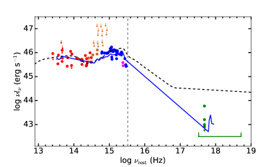
Figure 5.— Combined SEDs of the seven RSBALs. The IR-to-X-ray SED data are from WISE (red), 2MASS (brown), SDSS (blue), GALEX (magenta), and Chandra (green). The green segment represents the Chandra bandpass in the rest frame with an average redshift ($z$ = 1.747) of our targets. The Galactic extinction has been corrected for each band. All of our targets have been normalized to the composite SED (dashed line) of optically luminous quasars (Richards et al., 2006) at 3000 Å (corresponding to $10^{15}$ Hz). The data points from GALEX and SDSS u-band for quasars with redshifts above 0.9 and 2.2, respectively, are removed due to the possible presence of a Lyman break feature at rest-frame 912 Å (the vertical dashed line at $3.3\times 10^{15}$ Hz). The blue solid line represents the mean SED of BAL quasars from Gallagher et al. (2007). All of our RSBAL targets are significantly X-ray weak relative to the mean SED of normal quasars and are consistent with the mean SED of BAL quasars.

3.3. Radio Properties

The radio-loudness parameters ($R=f_{5~{}{\rm GHz}}$/$f_{\mbox{\scriptsize 4400 \AA}}$; Kellermann et al., 1989) of our seven targets are shown in Table 3. All of our targets are radio-quiet quasars with $R<10$. The flux densities at rest-frame 5 GHz were computed from the Faint Images of the Radio Sky at Twenty-centimeters (FIRST; Becker et al., 1995) survey at 1.4 GHz assuming a radio power-law index of $-0.5$ (Kellermann et al., 1989). Since our targets are not listed in the FIRST catalog, we estimate upper limits for their flux densities at 1.4 GHz as $0.25+3\sigma$ mJy, where $\sigma$ is the RMS noise and 0.25 mJy represents the CLEAN bias (White et al., 1997). The flux densities at rest-frame 4400 Å were converted from the flux densities at rest-frame of 2500 Å, using an assumed value of the optical power-law index of $-0.5$ (Schmidt & Green, 1983).

4. Discussion: X-RAY Assessment of Models For Redshifted BAL Quasars

Based upon the above multi-wavelength data analyses, all of our RSBAL quasars are significantly X-ray weak. In this section, we will utilize the X-ray results to assess the rotationally-dominated outflow model, the infall model, and the binary quasar model; see §1 for brief details of each model. As we will discuss in more detail below, the X-ray weakness of RSBAL quasars can be naturally explained by the rotationally-dominated outflow model, and it can also plausibly be described by the infall model with some additional constraints upon aspects of this model. However, the X-ray weakness cannot be easily explained by the binary quasar model.

4.1. Rotationally-Dominated Outflow Model

The rotationally-dominated outflow model adopts the standard accretion-disk wind structure commonly used to explain the properties of BAL quasars generally (e.g., Murray et al., 1995; Proga et al., 2000), preferring also a highly inclined system so that the rotational velocity can dominate the observed outflow dynamics (see §1). A key aspect of the standard model is the presence of X-ray absorbing shielding gas located at the base of the UV-absorbing wind, likely consisting of optically thick material that fails to reach escape velocity due to over-ionization. Our X-ray results provide evidence to support the existence of such shielding gas in RSBAL quasars.

First, the X-ray weakness of our RSBAL quasars suggests the existence of a heavy X-ray absorber lying along the line of sight to the small-scale X-ray emitting region; this X-ray weakness has been demonstrated using $\alpha_{\rm ox}$, $\Delta\alpha_{\rm ox}$, and examination of SEDs (see §3). Furthermore, although the number of sources is small, the quantitative level of X-ray weakness for our RSBAL quasars is consistent with that for appropriately matched BAL quasars generally (see Figure 4). This finding suggests that the X-ray absorption levels in our RSBAL quasars and BAL quasars generally are similar.

Although the numbers of X-ray counts for our targets are too limited for spectral analysis, we have made a basic assessment of likely X-ray absorption levels considering their hardness ratios. If we adopt a standard underlying X-ray power-law spectrum with a photon index of $\Gamma=2.0$ (and fixed Galactic absorption from Table 1), we can estimate the level of neutral intrinsic absorption required to produce the observed hardness ratios (we consider neutral absorption since this allows straightforward basic comparisons with most previous works, although the shielding gas may not be neutral). For our four LoBAL quasars with useful hardness-ratio constraints (i.e., measurements or lower limits; see Table 2), the estimated neutral hydrogen column densities range from $N_{\rm{H}}\gtrsim 5\times 10^{22}$ cm^-2 to $N_{\rm{H}}\approx 4\times 10^{23}$ cm^-2 (values for each target are listed in Table 2). This wide range is partly due to the redshifts spanned by our targets. Absorption in this range is consistent with that often seen for shielding gas in BAL quasars generally ($N_{\rm{H}}\approx 10^{22}$–$10^{23.5}$ cm^-2; e.g., Gallagher et al., 2002, 2006; Fan et al., 2009), again suggesting that typical shielding gas is a good candidate for the X-ray absorber in RSBAL quasars.

In the context of accretion-disk wind models, LoBALs are generally expected to be observed when our line of sight passes especially close to the accretion disk (e.g., Murray et al., 1995; Proga et al., 2000; Higginbottom et al., 2013). There is, moreover, some observational evidence that this basic idea is correct, at least for many BAL quasars, based upon correlated variations of ionization levels, kinematics, and column densities found across BAL-quasar samples (e.g., Voit et al., 1993; Filiz Ak et al., 2014). Our X-ray data are supportive of the rotationally-dominated outflow model for RSBAL quasars, and this model can explain the observed redshifted UV absorption best for large inclinations. It is exactly for such orientations that LoBALs are most likely to be observed, potentially explaining in a natural manner the predilection of RSBAL quasars to show LoBALs in their spectra.

4.2. Infall Model

The infall model discussed by Hall et al. (2013) suggests the RSBALs arise in gas infalling to a few hundred Schwarzschild radii. This gas would likely need to be in the form of dense clumps in order to maintain a sufficiently low ionization level to produce the observed UV absorption transitions. A high density might arise from compression during infall by both ram pressure and radiation pressure (e.g., Baskin et al., 2014). In the version of this model discussed by Hall et al. (2013), one would not necessarily expect shielding gas to lie along the line of sight to the X-ray emitting region. However, it could be present in some cases depending upon, e.g., system orientation.

All seven of our targets show evidence for X-ray absorption at the levels expected for appropriately matched BAL quasars generally (see §3 and §4.1). This finding indicates that, at the least, some additional stipulations upon the infall model are likely needed to make it agree well with the X-ray data. For example, one might reasonably propose that significant small-scale infall can be observed via UV absorption only in directions where the X-ray/EUV emission from the quasar is blocked by shielding gas and does not over-ionize the infalling gas. Gas infalling in other directions, or to smaller radii and greater redshifted velocities, could plausibly end up sufficiently highly ionized to be observable only at X-ray wavelengths. Such gas may have been seen to date in at least one AGN (e.g., Giustini et al., 2017). The observed line of sight in that object appears to show absorption from redshifted highly ionized iron lines (likely Fe XXV and Fe XXVI). Modeling of these roughly suggests an ionized absorber column density of $\sim 3\times 10^{23}$ cm^-2 and redshifted velocity of $\sim$ 36,000 km s^-1. Furthermore, the majority of RSBAL quasars also possess blueshifted BALs in their UV spectra (see Table 1 and Hall et al., 2013). Given this point, X-ray shielding gas might indeed be expected along the line of sight in the context of the accretion-disk wind model, since it is needed to prevent over-ionization of the wind producing the blueshifted UV absorption.

Another possibility is that the X-ray absorption might arise in the same infalling dense clump producing the redshifted UV absorption. It is difficult to constrain this model quantitatively at present, although it might require somewhat of a coincidence for the absorption levels in the infalling clump to match those expected for the shielding gas. Furthermore, if the X-ray absorption arose in the infalling clump, this configuration would not naturally explain why blueshifted UV absorption so commonly accompanies redshifted absorption.

4.3. Binary Quasar Model

In the binary quasar model, we observe a BAL outflow from a closer, fainter quasar in the binary that is backlit by a more distant, brighter quasar. Thus, the dominant radiation observed is that from the more distant member of the binary, and this member is not generally expected to be a BAL quasar (or otherwise heavily X-ray absorbed). The distance between the UV-absorbing material along the line of sight and the nucleus of the closer, fainter quasar is typically expected to be much larger than the scale of the X-ray/EUV absorbing shielding gas (see §1), which resides at $\lesssim$ 0.01 pc in the accretion-disk wind model. One would then not expect any substantial X-ray absorption commonly to be present. Thus, the binary quasar model does not provide any natural explanation of the X-ray weakness/absorption found for all seven of our RSBAL quasars, so it is disfavored by the X-ray measurements for the RSBAL quasar population in general.

5. Summary and Future Work

We have presented the X-ray properties of seven RSBAL quasars observed by Chandra, and we have used the results to assess the available models for these objects. Our main results are the following:

1. We have compared the X-ray to optical/UV spectral energy distributions of our RSBAL quasars with those of non-BAL quasars (from, e.g., S06, J07, G08) using $\alpha_{\rm ox}$ and $\Delta\alpha_{\rm ox}$ values as well as examination of their SEDs. We find that all of our RSBAL quasars are notably X-ray weak compared to non-BAL quasars. Furthermore, the quantitative level of X-ray weakness for RSBAL quasars, ranging from a factor of $\approx 6$ to $\lower 2.0pt\hbox{$\,\buildrel\scriptstyle>\over{\scriptstyle\sim}\,$}50$, appears similar to that for appropriately matched BAL quasars generally. See Sections 3.1 and 3.2.

2. The stacked effective power-law photon index derived using the counts from the five detected RSBAL quasars is $\Gamma_{\rm eff}=0.5^{+0.5}_{-0.4}$. This effective photon index is much smaller than that typically found for radio-quiet quasars ($\Gamma\approx 2$), suggesting the presence of heavy X-ray absorption of $N_{\rm H}\approx 2\times 10^{23}$ cm^-2 on average. This column density is larger than required by the observed UV absorption alone. However, it is consistent with expectations for the shielding gas of accretion-disk wind models as well as measurements of X-ray absorption in BAL quasars generally. See Sections 2.3 and 4.1.

3. We have used the X-ray measurements to assess the available models for RSBAL quasars. The X-ray weakness of RSBAL quasars can be naturally explained by the rotationally-dominated outflow model, and this is our generally favored model. The high system inclinations preferred in this model may also naturally explain the prevalence of LoBALs in the spectra of RSBAL quasars. However, the X-ray weakness can also plausibly be explained by the infall model provided one posits that X-ray shielding material always lies along the line of sight where infall observable in the UV occurs. The X-ray weakness cannot be easily explained by the binary quasar model. See Section 4.

These X-ray observations have made an important step toward understanding the nature of RSBAL quasars, mainly by demonstrating that they are generally X-ray weak due to absorption by shielding gas (or some other optically thick material much like it). However, further work is required to determine the precise nature of RSBAL quasars, e.g., by discriminating more strongly between the rotationally-dominated outflow and the infall models. One promising approach involves continued spectroscopic monitoring of the absorption troughs of RSBAL quasars. As discussed in §5.3 of Hall et al. (2013), the rotationally-dominated outflow model makes the testable prediction that both redshifted and blueshifted absorption troughs should migrate redward as the flow rotates. Such systematic migration would not obviously be seen in the infall model, where instead one might expect stronger absorption variability at larger redshifted velocities (see §6.1 of Hall et al., 2013). Results from such ongoing spectroscopic monitoring of RSBAL quasars will be presented in N. S. Ahmed et al., in preparation.

Furthermore, additional systematic searches for new RSBAL quasars should be performed, now that the sample of SDSS $z$ $>$ 1.5 quasars with high-quality spectroscopy has been substantially enlarged relative to what was searched in Hall et al. (2013); e.g., see Pâris et al. (2017). At least 30 new RSBAL quasars should be discovered in such searches, and some of these should be suitably bright for further efficient Chandra observations.

We thank the referee for helpful feedback. We also thank S. M. McGraw for calculating optical flux densities by fitting SDSS spectra. We thank C.-T. Chen, C.J. Grier, M. Eracleous, E.D. Feigelson, F. Vito, J. Wu, and G. Yang for helpful discussions. We acknowledge financial support from Chandra X-ray Center grant GO5-16092X, NSF grant AST-1516784, and the V.M. Willaman Endowment. N.S.A. and P.B.H. acknowledge support from NSERC. B.L. acknowledges support from the National Natural Science Foundation of China grant 11673010 and the Ministry of Science and Technology of China grant 2016YFA0400702. N.F.A. acknowledges financial support from TUBITAK (115F037). P.P. and R.S. acknowledge support from IFCPR under project NO. 5504-B. Y.S. acknowledges support from an Alfred P. Sloan Research Fellowship.

References

- Allen et al. (2011) Allen, J. T., Hewett, P. C., Maddox, N., Richards, G. T., & Belokurov, V. 2011, MNRAS, 410, 860
- Arav et al. (2013) Arav, N., Borguet, B., Chamberlain, C., Edmonds, D., & Danforth, C. 2013, MNRAS, 436, 3286
- Baskin et al. (2014) Baskin, A., Laor, A., & Stern, J. 2014, MNRAS, 445, 3025
- Becker et al. (1995) Becker, R. H., White, R. L., & Helfand, D. J. 1995, ApJ, 450, 559
- Borguet et al. (2013) Borguet, B. C. J., Arav, N., Edmonds, D., Chamberlain, C., & Benn, C. 2013, ApJ, 762, 49
- Broos et al. (2007) Broos, P. S., Feigelson, E. D., Townsley, L. K., et al. 2007, ApJS, 169, 353
- Chartas et al. (2009) Chartas, G., Saez, C., Brandt, W. N., Giustini, M., & Garmire, G. P. 2009, ApJ, 706, 644
- Civano et al. (2010) Civano, F., Elvis, M., Lanzuisi, G., et al. 2010, ApJ, 717, 209
- Cohen et al. (2003) Cohen, M., Wheaton, W. A., & Megeath, S. T. 2003, AJ, 126, 1090
- Dai et al. (2008) Dai, X., Shankar, F., & Sivakoff, G. R. 2008, ApJ, 672, 108
- Eisenstein et al. (2011) Eisenstein, D. J., Weinberg, D. H., Agol, E., et al. 2011, AJ, 142, 72
- Fabian (2012) Fabian, A. C. 2012, ARA&A, 50, 455
- Fan et al. (2009) Fan, L. L., Wang, H. Y., Wang, T., et al. 2009, ApJ, 690, 1006
- Feigelson & Babu (2012) Feigelson, E. D., & Babu, G. J. 2012, Modern Statistical Methods for Astronomy: With R Applications (Cambridge University Press)
- Filiz Ak et al. (2014) Filiz Ak, N., Brandt, W. N., Hall, P. B., et al. 2014, ApJ, 791, 88
- Gallagher et al. (2002) Gallagher, S. C., Brandt, W. N., Chartas, G., & Garmire, G. P. 2002, ApJ, 567, 37
- Gallagher et al. (2006) Gallagher, S. C., Brandt, W. N., Chartas, G., et al. 2006, ApJ, 644, 709
- Gallagher et al. (2007) Gallagher, S. C., Hines, D. C., Blaylock, M., et al. 2007, ApJ, 665, 157
- Ganguly et al. (2001) Ganguly, R., Bond, N. A., Charlton, J. C., et al. 2001, ApJ, 549, 133
- Garmire et al. (2003) Garmire, G. P., Bautz, M. W., Ford, P. G., Nousek, J. A., & Ricker, Jr., G. R. 2003, in Proc. SPIE, Vol. 4851, X-Ray and Gamma-Ray Telescopes and Instruments for Astronomy., ed. J. E. Truemper & H. D. Tananbaum, 28–44
- Gibson et al. (2008) Gibson, R. R., Brandt, W. N., & Schneider, D. P. 2008, ApJ, 685, 773 (G08)
- Gibson et al. (2009) Gibson, R. R., Jiang, L., Brandt, W. N., et al. 2009, ApJ, 692, 758 (G09)
- Giustini et al. (2017) Giustini, M., Costantini, E., De Marco, B., et al. 2017, A&A, 597, A66
- Green & Mathur (1996) Green, P. J., & Mathur, S. 1996, ApJ, 462, 637
- Hall et al. (2002) Hall, P. B., Anderson, S. F., Strauss, M. A., et al. 2002, ApJS, 141, 267
- Hall et al. (2013) Hall, P. B., Brandt, W. N., Petitjean, P., et al. 2013, MNRAS, 434, 222
- Hamann et al. (2013) Hamann, F., Chartas, G., McGraw, S., et al. 2013, MNRAS, 435, 133
- Hewett & Foltz (2003) Hewett, P. C., & Foltz, C. B. 2003, AJ, 125, 1784
- Higginbottom et al. (2013) Higginbottom, N., Knigge, C., Long, K. S., Sim, S. A., & Matthews, J. H. 2013, MNRAS, 436, 1390
- Just et al. (2007) Just, D. W., Brandt, W. N., Shemmer, O., et al. 2007, ApJ, 665, 1004 (J07)
- Kellermann et al. (1989) Kellermann, K. I., Sramek, R., Schmidt, M., Shaffer, D. B., & Green, R. 1989, AJ, 98, 1195
- King (2014) King, A. 2014, Space Sci. Rev., 183, 427
- Kraft et al. (1991) Kraft, R. P., Burrows, D. N., & Nousek, J. A. 1991, ApJ, 374, 344
- Luo et al. (2013) Luo, B., Brandt, W. N., Alexander, D. M., et al. 2013, ApJ, 772, 153
- Luo et al. (2014) —. 2014, ApJ, 794, 70
- Luo et al. (2015) Luo, B., Brandt, W. N., Hall, P. B., et al. 2015, ApJ, 805, 122
- Miller et al. (2011) Miller, B. P., Brandt, W. N., Schneider, D. P., et al. 2011, ApJ, 726, 20
- Murray et al. (1995) Murray, N., Chiang, J., Grossman, S. A., & Voit, G. M. 1995, ApJ, 451, 498
- Pâris et al. (2017) Pâris, I., Petitjean, P., Ross, N. P., et al. 2017, A&A, 597, A79
- Park et al. (2006) Park, T., Kashyap, V. L., Siemiginowska, A., et al. 2006, ApJ, 652, 610
- Planck Collaboration et al. (2015) Planck Collaboration, Ade, P. A. R., Aghanim, N., et al. 2015, ArXiv e-prints, arXiv:1502.01589
- Proga & Kallman (2004) Proga, D., & Kallman, T. R. 2004, ApJ, 616, 688
- Proga et al. (2000) Proga, D., Stone, J. M., & Kallman, T. R. 2000, ApJ, 543, 686
- Richards et al. (2006) Richards, G. T., Lacy, M., Storrie-Lombardi, L. J., et al. 2006, ApJS, 166, 470
- Rogerson et al. (2016) Rogerson, J. A., Hall, P. B., Rodríguez Hidalgo, P., et al. 2016, MNRAS, 457, 405
- Schmidt & Green (1983) Schmidt, M., & Green, R. F. 1983, ApJ, 269, 352
- Skrutskie et al. (2006) Skrutskie, M. F., Cutri, R. M., Stiening, R., et al. 2006, AJ, 131, 1163
- Steffen et al. (2006) Steffen, A. T., Strateva, I., Brandt, W. N., et al. 2006, AJ, 131, 2826 (S06)
- Trammell et al. (2007) Trammell, G. B., Vanden Berk, D. E., Schneider, D. P., et al. 2007, AJ, 133, 1780
- Trump et al. (2006) Trump, J. R., Hall, P. B., Reichard, T. A., et al. 2006, ApJS, 165, 1
- Voit et al. (1993) Voit, G. M., Weymann, R. J., & Korista, K. T. 1993, ApJ, 413, 95
- Weymann et al. (1991) Weymann, R. J., Morris, S. L., Foltz, C. B., & Hewett, P. C. 1991, ApJ, 373, 23
- White et al. (1997) White, R. L., Becker, R. H., Helfand, D. J., & Gregg, M. D. 1997, ApJ, 475, 479
- Wright et al. (2010) Wright, E. L., Eisenhardt, P. R. M., Mainzer, A. K., et al. 2010, AJ, 140, 1868
- Wu et al. (2011) Wu, J., Brandt, W. N., Hall, P. B., et al. 2011, ApJ, 736, 28
- Xue et al. (2011) Xue, Y. Q., Luo, B., Brandt, W. N., et al. 2011, ApJS, 195, 10
- York et al. (2000) York, D. G., Adelman, J., Anderson, Jr., J. E., et al. 2000, AJ, 120, 1579