Translation-invariant probability measures on entire functions

Abstract

We study non-trivial translation-invariant probability measures on the space of entire functions of one complex variable. The existence (and even an abundance) of such measures was proven by Benjamin Weiss. Answering Weiss’ question, we find a relatively sharp lower bound for the growth of entire functions in the support of such measures. The proof of this result consists of two independent parts: the proof of the lower bound and the construction, which yields its sharpness. Each of these parts combines various tools (both classical and new) from the theory of entire and subharmonic functions and from the ergodic theory.

We also prove several companion results, which concern the decay of the tails of non-trivial translation-invariant probability measures on the space of entire functions and the growth of locally uniformly recurrent entire and meromorphic functions.

1 Introduction and main results

Our starting point is Benjamin Weiss’ work [9] where he showed that there exist non-trivial translation-invariant probability measures on the space of entire functions of one complex variable (a formal definition of such measures will be given several lines below). Actually, Weiss showed that there is an abundance of such measures. Another approach to the construction of such measures was suggested by Tsirelson [8]. Tsirelson worked in a somewhat different and simpler context. The works of Weiss and Tsirelson raise a number of intriguing questions which lie at the crossroads of complex analysis and ergodic theory. Here, we address some of these questions.

1.1

Let $\mathcal{E}$ denote the space of entire functions with the topology generated by the semi-norms

$$\|F\|_{K}=\max_{K}|F|\,$$

where $K$ runs over all compact subsets of $\mathbb{C}$, and let $B$ be the Borel sigma-algebra generated by this topology. Then $\mathbb{C}$ acts on $(\mathcal{E},B)$ by translations:

$$(\tau_{w}F)(z)=F(z+w),\quad w\in\mathbb{C}\,.$$

The probability measure $\lambda$ on $(\mathcal{E},B)$ is called translation-invariant if it is invariant with respect to this action. The translation-invariant measure $\lambda$ is called non-trivial if the set of all constant functions in $\mathcal{E}$ has measure zero (the constant functions are fixed points of the action $\tau$). Due to [9], we know that non-trivial translation invariant probability measures on $(\mathcal{E},B)$ exist. In what follows, we retain the notation $\lambda$ for such measures.

After some reflection it becomes plausible that entire functions from the Borel support of $\lambda$ must grow sufficiently fast and that $\lambda$ must have heavy tails. The goal of this work is to justify these statements.

1.2

For an entire function $F$ we put

$$M_{F}(R)=\max_{R\,\overline{\mathbb{D}}}|F|\,,$$

where $R\,\overline{\mathbb{D}}=\{z\colon|z|\leqslant R\}$.

Theorem 1.

(A) Let $\lambda$ be a non-trivial translation-invariant probability measure on the space of entire functions. Then, for $\lambda$-a.e. function $F$ and for every $\varepsilon>0$,

$$\lim_{R\to\infty}\frac{\log\log M_{F}(R)}{\log^{2-\varepsilon}R}=+\infty\,.$$

(B) There exists a non-trivial translation-invariant probability measure on the space of entire functions such that, for $\lambda$-a.e. function $F$ and for every $\varepsilon>0$,

$$\lim_{R\to\infty}\frac{\log\log M_{F}(R)}{\log^{2+\varepsilon}R}=0\,.$$

1.2.1

The proof of the first part of Theorem 1 relies on a growth estimate of subharmonic functions, which might be of independent interest. To bring this estimate we introduce some notation.

• Till the end of Section 1.2.1, we assume that all squares denoted by $Q$ and $S$ have all four vertices with integer-valued coordinates.

Let $u$ be a non-negative subharmonic function on a neighbourhood of the square $Q\subset\mathbb{C}$ with side-length $L(Q)$. Let $M_{u}(Q)=\max_{\bar{Q}}u$ and $Z_{u}=\{u=0\}$. We denote by $A$ the area measure and by $|X|$ the cardinality of a finite set $X$.

Given $\gamma\in(0,1)$, we say that a unit square $S$ (i.e., the square with $L(S)=1$) is $\gamma$-good if (i) $A(S\cap Z_{u})\geqslant\gamma$ and (ii) $M_{u}(S)~{}\geqslant~{}1$. For any square $Q$, we put

$$\beta(Q)=\beta_{u,\gamma}(Q)=\frac{\bigl{|}\{S\subset Q\colon S\ {\rm is\ }\gamma{\rm-good\ unit\ square}\}\bigr{|}}{A(Q)}\,.$$

Lemma 1.

Given $\gamma,\beta\in(0,1)$ there exists $c=c(\gamma,\beta)>0$ such that for any square $Q$ with $L(Q)=L\geqslant 10$ and any non-negative subharmonic function $u$ on a neighbourhood of $Q$ with $\beta=\beta(Q)$,

$$M_{u}(Q)\geqslant e^{c\left(\frac{\log L}{\log\log L}\right)^{2}}\,.$$

It is instructive to juxtapose this estimate with a less restrictive one (which also will be used below), where we require that almost every unit square $S\subset Q$ contains a non-negligible piece of the set $Z_{u}$ and get a much faster growth of $u$.

Lemma 2.

Let $u$ be a non-negative subharmonic function on a neighbourhood of the square $Q$ with $L=L(Q)$ and let $\alpha>0$ be a positive parameter. Suppose that for some $\gamma\in(0,1)$ and for all, except of at most $\alpha L$ unit squares $S\subset Q$, we have $A(S\cap Z_{u})\geqslant\gamma$. Then,

$$M_{u}(Q)\geqslant e^{cL}M_{u}\bigl{(}[-\tfrac{1}{2},\tfrac{1}{2}]^{2}\bigr{)}$$

with some $c=c(\gamma,\alpha)>0$, provided that the size $L$ of the square $Q$ is sufficiently large.

Note that our reduction of the first part of Theorem 1 to Lemma 1 is based on the pointwise ergodic theorem, and that the proof of Lemma 1 makes use of Lemma 2.

1.2.2

A natural idea to construct a non-trivial translation-invariant probability measure on $\mathcal{E}$ (and, in particular, for the proof of the second part of Theorem 1) is to use the classical Krylov-Bogolyubov construction. We take a function $F\in\mathcal{E}$, denote by $\delta_{F}$ the point mass on $F$ (viewed as a probability measure on $\mathcal{E}$) and average it along the orbit of $\tau$ defining

$$\lambda_{R}=\frac{1}{\pi R^{2}}\,\int_{R\,\mathbb{D}}\delta_{\tau_{w}F}\,{\rm d}A(w)\,,\quad R\geqslant 1\,.$$

In other words, for any Borel set $B\subset\mathcal{E}$,

$$\lambda_{R}(B)=\frac{1}{\pi R^{2}}\,\int_{R\,\mathbb{D}}{1\hskip-2.5pt{\rm l}}_{B}(\tau_{w}F)\,{\rm d}A(w)\,.$$

Then, we let $R\to\infty$, and consider the limiting measure. The problem with this idea is that the space $\mathcal{E}$ is not compact; therefore, we need to ensure tightness of the family $(\lambda_{R})_{R\geqslant 1}$. In addition, we must ensure that (at least a part of) the limiting measure is not supported by the constant functions. Thus, the entire function $F$, which we start with, should be carefully chosen.

First, we construct a particular subharmonic function $u$ which can be thought as a certain approximation to $\log|F|$. We define a special unbounded closed set $E\subset\mathbb{C}$ which can be thought as a two-dimensional fat Cantor-type set viewed from the inside-out and a subharmonic function $u$ of a nearly minimal growth outside $E$ (Lemma 6). Then, using Hörmander’s classical estimates of solutions to $\bar{\partial}$-equations, we build an entire function $G$ of a nearly minimal growth outside $E$ with needed properties (Lemma 5). The functions $u$ and $G$ enjoy an interesting dynamical behaviour, and their construction is likely of independent interest.

1.3

We say that an entire function $F$ is locally uniformly recurrent if for every $\varepsilon>0$ and every compact set $K\subset\mathbb{C}$ the set $\bigl{\{}w\in\mathbb{C}\colon\max_{K}|\tau_{w}F-F|<\varepsilon\bigr{\}}$ is relatively dense in $\mathbb{C}$ (that is, any disk of sufficiently large radius contains at least one point of this set). This is a locally uniform counterpart of Bohr’s classical definition of almost-periodicity. In [9], Weiss gave a simple construction of functions of this class based on the Runge approximation theorem.

Locally uniformly recurrent entire functions can serve as a starting point for the Krylov-Bogolyubov-type construction described above. However, as the following theorem shows their growth is rather far from the minimal one.

Theorem 2.

(A) For any non-constant locally uniformly recurrent entire function $F$,

$$\liminf_{R\to\infty}\frac{\log\log M_{F}(R)}{R}>0\,.$$

(B) There exists a non-constant locally uniformly recurrent functions $F$ such that

$$\limsup_{R\to\infty}\frac{\log\log M_{F}(R)}{R}<\infty\,.$$

Note that the difference in the growth of entire functions in Theorems 1 and 2 and that of the corresponding subharmonic functions in Lemmas 1 and 2 are closely related.

1.4

As we have already mentioned, translation-invariant probability measures on the space of entire functions must have heavy tails.

Theorem 3.

(A) Let $\lambda$ be a non-trivial translation-invariant probability measure on the space of entire functions. Then, for every $\varepsilon>0$,

$$\mathbb{E}\bigl{[}(\log\log|F(0)|)^{1+\varepsilon}\bigr{]}=+\infty\,.$$

(B) There exists a non-trivial translation-invariant probability measure $\lambda$ on the space of entire functions such that, for every $t\geqslant 1$,

$$\lambda\bigl{\{}F\colon\log\log|F(0)|>t\bigr{\}}\lesssim\frac{1}{t}\,.$$

Here and elsewhere, the notation $X\lesssim Y$ means that there exists a positive numerical constant $C$ such that $X\leqslant CY$.

1.5

It is natural to look at the counterparts of Theorems 1 and 2 for meromorphic functions. We treat meromorphic functions as maps of the complex plane into the Riemann sphere endowed with the spherical metric $\rho$, and denote by $\mathcal{M}$ the space of meromorphic functions endowed with the topology of the locally uniform convergence in the spherical metric (as usual, we treat $\infty$ as a constant meromorphic function). By $B$ we denote the Borel sigma-algebra generated by this topology. Since $\mathcal{E}\subset\mathcal{M}$, it is worthwhile to note that these definitions are consistent with the ones we have used above.

To measure the growth of a meromorphic function $F$ we will use Nevanlinna’s characteristics $T_{F}(R)$. It will be convenient to use it in the Ahlfors-Shimizu geometric form:

$$T_{F}(R)=\int_{0}^{R}\Bigl{(}\frac{1}{\pi}\,\int_{r\,\mathbb{D}}F^{\#}(z)^{2}\,{\rm d}A(w)\Bigr{)}\,\frac{{\rm d}r}{r}\,,$$

where

$$F^{\#}(z)=\frac{|F^{\prime}(w)|}{1+|F(w)|^{2}}$$

is the spherical derivative of $F$. Then the inner integral in the definition of characteristics $T_{F}$ is the spherical area of the image of the disk $F(r\,\mathbb{D})$ considered with multiplicities of covering. The basic properties of the Nevanlinna’s characteristics can be found, for instance, in [6, Chapter 1]. Here, we will mention that if $F$ is an entire function then the growth of its Nevanlinna characteristics and of the logarithm of its maximum modulus are equivalent in the following sense:

$$T_{F}(R)<\log M_{F}(R)+O(1)\,,$$

and, for every $R_{1}>R$,

$$\log M_{F}(R)<\frac{R_{1}+R}{R_{1}-R}\,T_{F}(R_{1})+O(1)\,.$$

We also point out that it is easy to see that if $F$ is a non-constant doubly periodic meromorphic function, then the spherical area of the image $F(r\,\mathbb{D})$ counted with multiplicities has quadratic grows with $r$, and therefore, $T_{F}(R)$ has quadratic growth as well.

As above, $\mathbb{C}$ acts on $\mathcal{M}$ by translations. We call the probability measure $\lambda$ on $(\mathcal{M},B)$ translation-invariant if it is invariant with respect to this action. As above, we call a translation-invariant measure $\lambda$ non-trivial if the set of all non-constant functions has measure zero. Examples of non-trivial translation-invariant probability measures can be easily constructed by averaging the translations of a doubly periodic function. In these examples, for $\lambda$-a.e. function $F\in\mathcal{M}$, $T_{F}(R)=O(R^{2})$ as $R\to\infty$. The following theorem shows that one cannot do better:

Theorem 4.

Let $\lambda$ be a non-trivial translation-invariant probability measure on meromorphic functions. Then, for $\lambda$-a.e. function $F\in\mathcal{M}$,

$$\liminf_{R\to\infty}\frac{T_{F}(R)}{R^{2}}>0\,.$$

We call a meromorphic function $F$ locally uniformly recurrent if for every $\varepsilon>0$ and every compact set $K\subset\mathbb{C}$, the set $\bigl{\{}w\in\mathbb{C}\colon\max_{K}\rho(\tau_{w}f,f)<\varepsilon\bigr{\}}$ is relatively dense in $\mathbb{C}$. Here, as above, $\rho$ is the spherical distance. It is easy to see that doubly periodic meromorphic functions are locally uniformly recurrent. I.e., there are plenty of locally uniformly recurrent meromorphic functions $F$ with $T_{F}(R)=O(R^{2})$ as $R\to\infty$. As in the previous case, this estimate cannot be improved:

Theorem 5.

Let $F$ be a non-constant locally uniformly recurrent meromorphic function. Then

$$\liminf_{R\to\infty}\frac{T_{F}(R)}{R^{2}}>0\,.$$

Acknowledgments

The authors are grateful to Alexander Borichev, Gady Kozma, Fedor Nazarov and Benjy Weiss for several very helpful discussions. We thank Steven Britt for his assistance with language editing.

2 Proof of Lemmas 1 and 2

In this section the squares denoted by $Q$, $Q_{j}$, $\mathcal{Q}$, and $S$ have vertices with integer-valued coordinates, $Q$ is a square with large side-length $L=L(Q)$, and $u$ is a subharmonic function on a neighbourhood of $Q$. By $Z_{u}=\{u=0\}$ we denote the zero set of $u$.

2.1 Proof of Lemma 2

Assuming that for all but $\alpha L$ unit squares $S\subset Q$ we have $A(S\cap Z_{u})\geqslant\gamma$, we need to show that

$$\max_{Q}u\geqslant e^{c(\alpha,\gamma)L}\max_{[-1/2,1/2]^{2}}u\,.$$

First, we observe that if the disk $D_{z}\subset Q$ centered at $z$ contains a portion of the zero set $Z_{u}$ of area at least $\gamma$ (with $\gamma<A(D_{z})$), then

$$u(z)\leqslant\frac{1}{A(D_{z})}\,\int_{D_{z}}u\,{\rm d}A=\frac{1}{A(D_{z})}\,\int_{D_{z}\setminus Z_{u}}u\,{\rm d}A\leqslant\bigl{(}1-\frac{\gamma}{A(D_{z})}\bigr{)}\,\max_{\bar{D}_{z}}u\,,$$

whence,

$$\max_{\bar{D}_{z}}u\geqslant\Bigl{(}1-\frac{\gamma}{A(D_{z})}\Bigr{)}^{-1}u(z)\,.$$

Let $N$ be the integer part of $\tfrac{1}{2}L$. Put $M_{u}(r)\stackrel{{\scriptstyle\rm def}}{{=}}\max\bigl{\{}u(z)\colon|z|\leqslant r\bigr{\}}$, take the points $z_{0}=0$, $z_{1}$, …, $z_{N}$, with $|z_{j}|=j$, so that $u(z_{j})=M_{u}(j)$, $j=1,\ldots,N$, and consider the disks $D_{j}=D(z_{j},p)$ with sufficiently large integer $p\geqslant 2$. We call the index $j\leqslant N-p$ normal if the disk $D_{j}$ contains at least one non-exceptional unit square $S$. For normal indices $j$, we have

$$M_{u}(j+p)\geqslant\max_{\bar{D}_{j}}u\geqslant\Bigl{(}1-\frac{\gamma}{\pi p^{2}}\Bigr{)}^{-1}u(z_{j})=\Bigl{(}1-\frac{\gamma}{\pi p^{2}}\Bigr{)}^{-1}M_{u}(j)\,.$$ (1)

If the disks $D_{j_{1}}$, …, $D_{j_{\ell}}$ are not normal, then the number of different exceptional squares contained in their union $D_{j_{1}}\bigcup\ldots\bigcup D_{j_{\ell}}$ is $\gtrsim\ell p$. Since the total number of exceptional unit squares does not exceed $\alpha L$, we conclude that the number of not normal disks is $\lesssim\alpha p^{-1}L<\tfrac{1}{5}L$ provided that $p$ was chosen much larger than $\alpha$. We conclude that there are at least $\tfrac{1}{4}L$ indices $1\leqslant j\leqslant N-p$, for which estimate (1) holds. Hence, the lemma follows. $\Box$

2.2 Proof of Lemma 1

Recall that we say that a unit square $S\subset Q$ is $\gamma$-good if $A(S\cap Z_{u})\geqslant\gamma$ and $\max_{S}u\geqslant 1$, and that for any square $Q$, we put

$$\beta(Q)=\frac{\bigl{|}\{S\subset Q\colon S\ {\rm is\ }\gamma{\rm-good\ unit\ square}\}\bigr{|}}{A(Q)}\,.$$

Our aim is to show that

$$\log\max_{Q}u\geqslant c(\beta,\gamma)\Bigl{(}\frac{\log L}{\log\log L}\Bigr{)}^{2},\quad\beta=\beta(Q)\,.$$

With no loss of generality we assume that $L=k^{k}$ for an integer $k$ (then, $k\simeq\tfrac{\log L}{\log\log L}$). We construct a sequence of squares $Q_{0}=Q$, …, $Q_{k}$, with $L(Q_{j})=k^{k-j}$. First, we split the square $Q_{j-1}$ into $k^{2}$ squares $\mathcal{Q}$ with $L(\mathcal{Q})=k^{k-j}$. For these squares $\mathcal{Q}$ we write $\mathcal{Q}\prec Q_{j-1}$, and note that

$$\beta(Q_{j-1})=\frac{1}{k^{2}}\,\sum_{\mathcal{Q}\prec Q_{j-1}}\beta(\mathcal{Q})\,.$$ (2)

Then, according to certain rules described below, we choose one of the squares $\mathcal{Q}$, and call it $Q_{j}$.

Suppose that the squares $Q_{0}$, …, $Q_{j-1}$ have already been chosen. We will fix the parameters $B>1$ and $0<\theta<1$ to be chosen later, and consider three cases.

Case 1: there exist at least $Bk$ squares $\mathcal{Q}\prec Q_{j-1}$ such that $\beta(\mathcal{Q})<\tfrac{1}{2}\beta(Q_{j-1})$.

We claim that in this case there exists at least one square $\mathcal{Q}\prec Q_{j-1}$ with

$$\beta(\mathcal{Q})\geqslant\Bigl{(}1+\frac{B}{2k}\Bigr{)}\beta(Q_{j-1})\,.$$ (3)

Indeed, otherwise, (2) gives us

$$1\leqslant\frac{1}{k^{2}}\Bigl{(}Bk\cdot\frac{1}{2}+(k^{2}-Bk)\cdot\Bigl{(}1+\frac{B}{2k}\Bigr{)}\Bigr{)}=\frac{1}{k^{2}}\bigl{(}k^{2}-\tfrac{1}{2}B^{2}\bigr{)}<1\,,$$

arriving at a contradiction.

Then, we let $Q_{j}$ be one of the squares $\mathcal{Q}\prec Q_{j-1}$ such that (3) holds.

Case 2: for all squares $\mathcal{Q}\prec Q_{j-1}$ contained in the square $(1-\theta)Q_{j-1}$,

$$\beta(\mathcal{Q})<\bigl{(}1-\frac{1}{k}\bigr{)}\beta(Q_{j-1})\,.$$

Here, $(1-\theta)Q_{j-1}$ denotes the square with the same center as $Q_{j-1}$ and $L((1-\theta)Q_{j-1})=(1-\theta)L(Q_{j-1})$.

We claim that if $\theta$ is chosen sufficiently small, then (3) holds for at least one of the remaining squares. Otherwise,

$$1<\frac{1}{k^{2}}\Bigl{(}(1-\theta)^{2}k^{2}\cdot\Bigl{(}1-\frac{1}{k}\Bigr{)}+\bigl{(}1-(1-\theta)^{2}\bigr{)}k^{2}\cdot\Bigl{(}1+\frac{B}{2k}\Bigr{)}\Bigr{)}\\ =\frac{1}{k^{2}}\Bigl{(}k^{2}-k\bigl{(}(1-\theta)^{2}-\tfrac{1}{2}B(1-(1-\theta)^{2}\bigr{)}\Bigr{)}<1-\frac{1}{k}\bigl{(}(1-\theta)^{2}-B\theta\bigr{)}<1\,,$$

provided that $B\theta<\tfrac{1}{2}$.

As in the first case, we let $Q_{j}$ be one of the squares $\mathcal{Q}\prec Q_{j-1}$ such that (3) holds.

We now consider the remaining case, which is complementary to the cases 1 and 2:

Case 3: there exists at least one square $\mathcal{Q}\prec Q_{j-1}$ contained in $(1-\theta)Q_{j-1}$ such that $\beta(\mathcal{Q})\geqslant\bigl{(}1-\tfrac{1}{k}\bigr{)}\beta(Q_{j-1})$ (with $\theta=\theta(B)$ chosen above). At the same time, the number of squares $Q\prec Q_{j-1}$ with $\beta(Q)\geqslant\frac{1}{2}\beta(Q_{j-1})$ is not less than $k^{2}-Bk$.

Then we call one one these squares $Q_{j}$. We also know that for at most $Bk$ squares $Q\prec Q_{j-1}$, we have $\beta(Q)\leqslant\tfrac{1}{2}\beta(Q_{j-1})$.

Now, we are ready to prove Lemma 1. First, we note that on each step the value $\beta(Q_{j})$ either increases (cases 1 and 2), or decreases by a factor of at most $1-\tfrac{1}{k}$. Since the total number of steps is $k\geqslant 2$, we conclude that for each $j$, $\beta(Q_{j})\geqslant\tfrac{1}{3}\beta(Q_{0})=\tfrac{1}{3}\beta$.

Next, we observe that if on the $j$th step one of the cases 1 or 2 occurs, then by (3), $\beta(Q_{j})$ will increase by a factor of at least $1+(2k)^{-1}B$. Since on other steps $\beta(Q_{j})$ decreases not more than a factor of $1-\tfrac{1}{k}$, choosing $B=B(\beta)$ sufficiently large, ensures us that out of the $k$ steps at least $k/2$ steps result in case $3$.

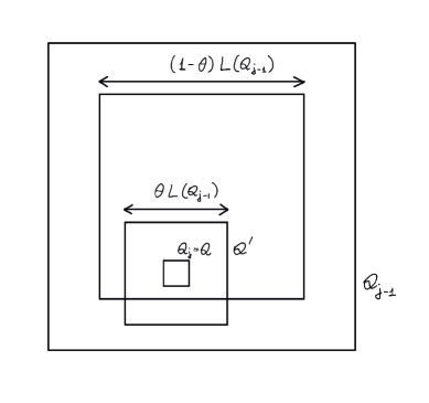
Figure 1:

The squares $Q_{j-1}$ and $Q_{j}$ in the 3rd case.

Assume that on the $j$th step the 3rd case happens. Then, applying Lemma 2 (with an appropriate scaling) to the square $Q^{\prime}$ with $L(Q^{\prime})=\theta L(Q_{j-1})$ centered at the same point as $Q_{j}$ (and therefore, contained in $Q_{j-1}$), we obtain

$$M_{u}(Q_{j-1})\geqslant M_{u}(Q^{\prime})\geqslant e^{ck}M_{u}(Q_{j})$$

with some $c=c(\gamma,\beta)$. Since this happens for at least $k/2$ indices $j$, we conclude that

$$M_{u}(Q_{0})\geqslant e^{ck^{2}}M_{u}(Q_{k})\,.$$

It remains to recall that $k\simeq\tfrac{\log L}{\log\log L}$ and that, since $Q$ was a good square, $M_{u}(Q_{k})\geqslant 1$. $\Box$

3 Proof of Theorems 1A and 2A

In this section, $S_{\rho}(z)$ denotes the square of side-length $\rho$ centered at $z$, and we let $S_{\rho}=S_{\rho}(0)$.

3.1 An integral-geometric lemma

We will be using a simple and known fact from the integral geometry:

Lemma 3.

For any measurable set $X\subset\mathbb{C}$ and any $0<\rho<R$,

$$\Bigl{|}\,\frac{A(S_{R}\cap X)}{A(S_{R})}-\frac{1}{A(S_{R})}\,\int_{S_{R}}\frac{A(S_{\rho}(z)\cap X)}{A(S_{\rho})}\,{\rm d}A(z)\,\Bigr{|}\lesssim\frac{\rho}{R}\,.$$

3.2 Proof of Theorem 1A

3.2.1

Applying the ergodic decomposition theorem (see, for instance, [5, Sections 6.1 and 8.6]), we can find a Borel probabity space $(\Omega,\mathcal{F},\nu)$ and a measurable map $\omega\mapsto\lambda_{\omega}$ for which

(i) for $\nu$-a.e. $\omega$, $\lambda_{\omega}$ is a probability measure on $(\mathcal{E},B)$, which is invariant and ergodic with respect to the action of $\mathbb{C}$ on $(\mathcal{E},B)$ by translations $\tau$;

(ii) for every Borel set $\mathcal{X}\in B$,

$$\lambda(\mathcal{X})=\int_{\Omega}\lambda_{\omega}(\mathcal{X})\,{\rm d}\nu(\omega)\,.$$

It is not difficult to see that the set of entire functions $F$ such that, for every $\varepsilon>0$,

$$\lim_{R\to 0}\,\frac{\log\log M_{F}(R)}{\log^{2-\varepsilon}R}=+\infty$$

is a Borel set. Hence, proving Theorem 1A, it suffices to assume that the measure $\lambda$ is ergodic with respect to translations $\tau$.

3.2.2

Put $X(F)=\{z\in\mathbb{C}\colon|F(z)|\leqslant 1\}$. Given $\rho>1$, consider the Borel sets

$$\mathcal{E}_{1}(\rho)=\{F\in\mathcal{E}\colon A(S_{\rho}\cap X(F))\geqslant 1\}\,,\quad\mathcal{E}_{2}(\rho)=\{F\in\mathcal{E}\colon\max_{\bar{S}_{\rho}}|F|\geqslant e\}\,.$$

For $\rho<\rho^{\prime}$, we have $\mathcal{E}_{i}(\rho)\subset\mathcal{E}_{i}(\rho^{\prime})$, $i=1,2$. We denote by $\mathcal{E}_{i}(\infty)$, $i=1,2$, the corresponding limiting sets as $\rho\to\infty$. Since the complement $\mathcal{E}\setminus\mathcal{E}_{2}(\infty)$ consists of constant functions and the measure $\lambda$ does not charge constants, $\lambda(\mathcal{E}_{2}(\infty))=1$.

3.2.3

We claim that $\lambda(\mathcal{E}_{1}(\infty))=1$ as well. Otherwise, by translation-invariance of the set $\mathcal{E}_{1}(\infty)$ and by ergodicity of $\lambda$, we have $\lambda(\mathcal{E}_{1}(\infty))=0$. Applying Lemma 3, we conclude that for $\lambda$-a.e. $F$ and for every $\rho>0$,

$$\lim_{R\to\infty}\frac{1}{A(S_{R})}\,\int_{S_{R}}\frac{A(S_{\rho}(z)\cap X(F))}{A(S_{\rho})}\,{\rm d}A(z)=0\,.$$

Then, by the Wiener version of the pointwise ergodic theorem (see for instance, [1]) for every $\rho>1$,

$$\int_{\mathcal{E}}A(S_{\rho}\cap X(F))\,{\rm d}\lambda(F)=0\,,$$

i.e., for $\lambda$-a.e. $F\in\mathcal{E}$, $X(F)=\emptyset$, which means that $|F|\geqslant 1$ everywhere in $\mathbb{C}$. That is, $F$ a constant function, which is a contradiction.

3.2.4

Now, we fix $\rho>1$ so that $\lambda\bigl{(}\mathcal{E}_{1}(\rho)\cap\mathcal{E}_{2}(\rho)\bigr{)}\geqslant\frac{9}{10}$, and let

$$X(F,\rho)=\{z\in\mathbb{C}\colon A(S_{\rho}(z)\cap X(F))\geqslant 1,\,\max_{S_{\rho}(z)}|F|\geqslant e\}\,.$$

We claim that for $\lambda$-a.e. $F\in\mathcal{E}$, the limit

$$\lim_{R\to\infty}\frac{A(S_{R}\cap X(F,\rho))}{A(S_{R})}$$

exists and is $\geqslant\frac{9}{10}$. Indeed, for any $F\in\mathcal{E}$ and any $r>1$, by Lemma 3, we have

$$\frac{A(S_{R}\cap X(F,\rho))}{A(S_{R})}=\frac{1}{A(S_{R})}\,\int_{S_{R}}\frac{A(S_{r}(z)\cap X(F,\rho))}{A(S_{r})}\,{\rm d}A(z)+O\bigl{(}\frac{r}{R}\bigr{)}\,,$$

and by the pointwise ergodic theorem, for $\lambda$-a.e. $F$, the $R\to\infty$ limit of the RHS exists and equals

$$\int_{\mathcal{E}}\frac{A(S_{r}\cap X(F,\rho))}{A(S_{r})}\,{\rm d}\lambda(F)\,.$$

Applying Fubini’s theorem and then using the translation-invariance of the measure $\lambda$, we can rewrite this expression as

$$\frac{1}{A(S_{r})}\,\int_{S_{r}}\Bigl{[}\,\int_{\mathcal{E}}{1\hskip-2.5pt{\rm l}}_{X(F,\rho)}(z)\,{\rm d}\lambda(F)\,\Bigr{]}\,{\rm d}A(z)$$

$$\qquad=\frac{1}{A(S_{r})}\,\int_{S_{r}}\Bigl{[}\,\int_{\mathcal{E}}{1\hskip-2.5pt{\rm l}}_{X(\tau_{z}F,\rho)}(0)\,{\rm d}\lambda(F)\,\Bigr{]}\,{\rm d}A(z)$$

$$\qquad=\lambda\bigl{\{}F\in\mathcal{E}\colon 0\in X(F,\rho)\bigr{\}}$$

$$\qquad=\lambda\bigl{(}\mathcal{E}_{1}(\rho)\cap\mathcal{E}_{2}(\rho)\bigr{)}\geqslant\frac{9}{10}\,,$$

proving the claim.

3.2.5

It remains to show that if $F$ is a non-constant entire function such that for some $\rho>1$,

$$\liminf_{R\to\infty}\frac{A(S_{R}\cap X(F,\rho))}{A(S_{R})}\geqslant\frac{9}{10}\,,$$

then, for every $\varepsilon>0$,

$$\lim_{R\to\infty}\frac{\log\log M_{F}(R)}{\log^{2-\varepsilon}R}=+\infty\,.$$ (4)

First, we note that it suffices to show that (4) holds for the sequence $R_{n}=(2\rho)^{n}$; then the general case follows.

Then, we take $R=(2\rho)^{n}$ with sufficiently large $n$, split the square $S_{R}$ into $R^{2}/(2\rho)^{2}$ squares $S$ squares $\mathcal{S}$ with side-length $2\rho$, and consider the subharmonic function $u=\log_{+}|F|$. By the last claim, for at least half of the squares $\mathcal{S}$, $A(\mathcal{S}\cap Z_{u})\geqslant 1$ and $\max_{\bar{\mathcal{S}}}u\geqslant 1$. Applying Lemma 1, we complete the proof. $\Box$

3.2.6 Remark

Note that with a little effort one can extract from Lemma 1 slightly more than Theorem 1A asserts, namely, that for $\lambda$-a.e. $F\in\mathcal{E}$,

$$\liminf_{R\to\infty}\,\log\log M_{F}(R)\cdot\Bigl{(}\frac{\log\log R}{\log R}\Bigr{)}^{2}>0\,.$$

Likely, this estimate can be somewhat improved.

3.3 Proof of Theorem 2A

The proof is straightforward. Let $F$ be a non-constant locally uniformly recurrent function, and let $M=\max_{[0,1]^{2}}|F|$. Applying the definition of locally uniform recurrency with $K=[0,1]^{2}$ and $\varepsilon=1$, we see that there exists $L=L(M)$ such that for every square $Q$ with the side-length $L$, $A\bigl{(}Q\cap\{|F|\leqslant M+1\}\bigr{)}\geqslant 1$. Then, Lemma 2 does the job. $\Box$

4 Proof of Theorem 3A

4.1 A loglog-lemma that yields Theorem 3A

We will use a version of the classical Carleman-Levinson-Sjöberg loglog-theorem, cf. [2, 3, 4]. Likely, this lemma can be deduced from at least one of many known versions of the loglog-theorem. Since its proof is quite simple, for the reader’s convenience, we will supply it.

Lemma 4.

Suppose $u$ is a non-constant subharmonic function in $\mathbb{C}$. Then, for every $\varepsilon>0$,

$$\lim_{R\to\infty}\frac{1}{A(R\,\mathbb{D})}\,\int_{R\,\mathbb{D}}\bigl{(}\log_{+}u\bigr{)}^{1+\varepsilon}\,{\rm d}A=\infty\,.\\$$

This lemma immediately yields Theorem 3A: applying, as above, the ergodic decomposition theorem, we may assume that the measure $\lambda$ is ergodic. Then, by the pointwise ergodic theorem, for $\lambda$-a.e. entire function $F$ we have

$$\lim_{R\to\infty}\frac{1}{R^{2}}\,\int_{R\mathbb{D}}\bigl{(}\log_{+}\log_{+}|F(z)|\bigr{)}^{1+\varepsilon}\,{\rm d}A(z)=\mathbb{E}\bigl{[}(\log_{+}\log_{+}|F(0)|)^{1+\varepsilon}\bigr{]}\,,$$

and since the measure $\lambda$ does not charge constant functions, by Lemma 4, the limit on the RHS is infinite. $\Box$

4.2 Proof of Lemma 4

We let $M_{u}(R)=\max_{R\,\bar{\mathbb{D}}}u$ and choose $N$ so that $b^{N}<R\leqslant b^{N+1}$, with some $b>1$ to be chosen. For $1\leqslant j\leqslant N$, we take $z_{j}$, $|z_{j}|=R_{j}$, so that

$$u(z_{j})=M_{u}(R_{j})=b^{j},\quad j\in\mathbb{N}\,,$$

and let $R_{N+1}=R$. Then, we put $\rho_{j}=R_{j+1}-R_{j}$, $1\leqslant j\leqslant N$, let $D_{j}$ be the disks centered at $z_{j}$ of radius $\tfrac{1}{2}\rho_{j}$, and let $D_{j}^{+}=D_{j}\bigcap\{R_{j}\leqslant|z|\leqslant R_{j+1}\}$. Note that the sets $D_{j}^{+}$ are disjoint and that $A(D_{j}^{+})\geqslant\tfrac{1}{2}A(D_{j})$. We claim that

• If $b$ is chosen sufficiently close to $1$ and $c$ is sufficiently small, then for every $1\leqslant j\leqslant N$, $u(z)\geqslant cu(z_{j})$ on a subset $D_{j}^{\prime}\subset D_{j}^{+}$ with $A(D_{j}^{\prime})\geqslant\tfrac{1}{4}A(D_{j})$.

Indeed, let $D_{j}^{*}=\{z\in D_{j}\colon u(z)\geqslant cu(z_{j})\}$. Then,

$$b^{j}=u(z_{j}) \leqslant\frac{1}{A(D_{j})}\,\int_{D_{j}}u\,{\rm d}A$$

$$\leqslant\frac{1}{A(D_{j})}\,\bigl{(}cb^{j}(A(D_{j})-A(D_{j}^{*}))+b^{j+1}A(D_{j}^{*})\bigr{)}$$

$$=(b^{j+1}-cb^{j})\,\frac{A(D_{j}^{*})}{A(D_{j})}+cb^{j}\,,$$

whence

$$\frac{A(D_{j}^{*})}{A(D_{j})}\geqslant\frac{1-c}{b-c}>\frac{3}{4}$$

provided that $b>c$ and $3b+c<4$. It remains to put $D_{j}^{\prime}=D_{j}^{*}\bigcap D_{j}^{+}$.

Now,

$$\int_{R\mathbb{D}}(\log_{+}u)^{1+\varepsilon}\,{\rm d}A \geqslant\sum_{j=1}^{N}\int_{D_{j}^{\prime}}(\log_{+}u)^{1+\varepsilon}\,{\rm d}A$$

$$\gtrsim\sum_{j=1}^{N}j^{1+\varepsilon}A(D_{j}^{\prime})$$

$$\gtrsim\sum_{j=1}^{N}j^{1+\varepsilon}\rho_{j}^{2}\,.$$

Let $N_{0}\gg 1$. Then, for $N\gg N_{0}$,

$$\Bigl{(}\sum_{j=N_{0}}^{N}\rho_{j}\Bigr{)}^{2} <\sum_{j\geqslant N_{0}}\frac{1}{j^{1+\varepsilon}}\cdot\sum_{j=N_{0}}^{N}j^{1+\varepsilon}\rho_{j}^{2}$$

$$\lesssim N_{0}^{-\varepsilon}\,\sum_{j=N_{0}}^{N}j^{1+\varepsilon}\rho_{j}^{2}\,.$$

Letting $N\to\infty$, we get

$$\liminf_{R\to\infty}\frac{1}{A(R\mathbb{D})}\int_{R\mathbb{D}}(\log_{+}u)^{1+\varepsilon}\,{\rm d}A\gtrsim N_{0}^{\varepsilon}\,.$$

Then, letting $N_{0}\to\infty$, we conclude the proof. $\Box$

5 Proof of Theorems 4 and 5

Both proofs are quite straightforward.

5.1 Proof of Theorem 4

As in the previous proofs we may assume that the measure $\lambda$ is ergodic. Then, by the pointwise ergodic theorem, for $\lambda$-a.e. meromorphic function $F$,

$$\lim_{R\to\infty}\frac{1}{A(R\,\mathbb{D})}\,\int_{R\mathbb{D}}F^{\#}(z)^{2}\,{\rm d}A(z)=\mathbb{E}\bigl{[}F^{\#}(0)^{2}\bigr{]}\,.$$

Since $\lambda$-a.s., the function $F$ is not a constant (and the distribution of $\lambda$ is translation invariant), the RHS is positive (may be infinite). Thus, for sufficiently large $R$s,

$$\int_{R\mathbb{D}}F^{\#}(z)^{2}\,{\rm d}A(z)\gtrsim R^{2}\,,$$

and therefore, $T_{F}(R)\gtrsim R^{2}$. $\Box$

5.2 Proof of Theorem 5

Let $F$ be a non-constant locally uniformly recurrent meromorphic function. We fix a disk $D$ such that $F$ is analytic on $\bar{D}$, take the closed spherical disk $\bar{\mathfrak{D}}\subset F(D)$ such that $\bar{\mathfrak{D}}\cap F(\partial D)=\emptyset$, and denote by $\delta$ the spherical distance between $\bar{\mathfrak{D}}$ and the curve $F(\partial D)$.

By the definition of local uniform recurrency, each square $Q$ with sufficiently large length-side $L(Q)$ contains a point $w$ such that $\max_{\bar{D}}\rho(F,\tau_{w}F)<\tfrac{1}{2}\,\delta$, where $\rho$ is the spherical metric. Denote by $D_{w}$ the disk centered at $w$ of the same radius as $D$. We claim that $\mathfrak{D}\subset F(D_{w})$. To show this, fix a point $\zeta\in\mathfrak{D}\subset F(D)$. Then, by the argument principle, the index of the curve $F(\partial D)$ with respect to the point $\zeta$ is positive. Furthermore, when the point $z$ traverses the circumference $\partial D$, $F(z)$ traverses the curve $F(\partial D)$, $F(z+w)$ traverses the curve $F(\partial D_{w})$, and the spherical distance between $F(z)$ and $F(z+w)$ remains less than $\frac{1}{2}\,\delta$, while $\rho(\zeta,F(\partial D))\geqslant\delta$. Hence, the index of the curve $F(\partial D_{w})$ with respect to $\zeta$ coincides with that of $F(\partial D)$, and therefore, is positive as well. Thus, $\zeta\in F(D_{w})$ proving the claim.

Denote by $Q^{*}$ the square having the same center as $Q$ and with the length-side $L(Q^{*})=L(Q)+\operatorname{radius}(D)$. Since $D_{w}\subset Q^{*}$, we conclude that $\mathfrak{D}\subset F(Q^{*})$. Hence, the spherical area of $F(Q^{*})$ is not less than that of $\mathfrak{D}$. Packing the disk $R\mathbb{D}=\{|z|<R\}$ with sufficiently large $R$ by about $cR^{2}$ disjoint translations of the square $Q^{*}$, we see that the spherical area of $F(R\mathbb{D})$ is $\gtrsim R^{2}$, which yields the theorem. $\Box$

6 Entire functions of almost minimal growth outside a ternary system of squares

6.1 Ternary system of squares

We will construct the closed set $E\subset\mathbb{C}$ which we will call the ternary systems of squares. It will be defined as the limit of the increasing sequence $(E_{n})$ of compact sets such that $E_{n}$ consists of $E_{n-1}$ and its eight disjoint translations. One can think about the limiting set $E$ as a two-dimensional ternary Cantor-type set viewed from the inside-out.

6.1.1 Notation

For $X\subset\mathbb{C}$ and $\eta>0$, we put

$$X^{+\eta}=\bigl{\{}z\in\mathbb{C}\colon d_{\infty}(z,X)\leqslant\eta\bigr{\}},\quad X^{-\eta}=\bigl{\{}z\in\mathbb{C}\colon d_{\infty}(z,X^{c})\geqslant\eta\bigr{\}}\,.$$

Here and elsewhere, $d_{\infty}$ denotes the $\ell^{\infty}$-distance on $\mathbb{R}^{2}$.

For $X\subset\mathbb{C}$, we put $\tau_{w}X=\bigl{\{}z-w\colon z\in X\bigr{\}}$. That is, if the function $f$ is defined on $X$, then $\tau_{w}f$ is defined on $\tau_{w}X$.

6.1.2 Squares and corridors

We fix a sequence $(\varepsilon_{n})\downarrow 0$ and define:

• the increasing sequence $(a_{n})$ by $a_{0}=1$, $a_{n}=3a_{n-1}(1+\varepsilon_{n})$;

• the squares $S_{n}=[-a_{n},a_{n}]^{2}$;

• the translates $w_{j}(n)=a_{n-1}(2+3\varepsilon_{n})\omega_{j}$, where $\{\omega_{j}\}_{0\leqslant j\leqslant 8}=\{0,\pm 1,\pm{\rm i},\pm 1\pm{\rm i}\}$;

see Figure 2.

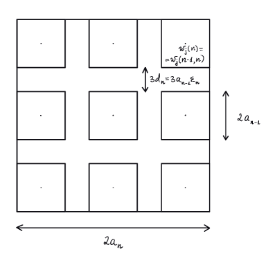
Figure 2:

The square $S_{n}$ with 9 copies of the square $S_{n-1}$.

Then, $E_{0}=S_{0}$, $E_{n}=\bigcup_{j=0}^{8}\tau_{w_{j}(n)}E_{n-1}$, and finally, $E=\bigcup_{n}E_{n}$.

For every $k<n$, the set $E_{n}$ consists of $9^{n-k}$ disjoint copies of $E_{k}$. We denote by $w_{j}(k,n)$, $0\leqslant j\leqslant 9^{n-k}-1$, the centers of these copies. That is, there exist indices $j_{1},\ldots,j_{n-k}\in\{0,1,\ldots,8\}$ such that

$$w_{j}(k,n)=w_{j_{1}}(k+1)+\ldots+w_{j_{n-k}}(n)$$

(in particular, $w_{j}(n-1,n)=w_{j}(n)$), and

$$E_{n}=\bigcup_{j_{n}=0}^{8}\ldots\bigcup_{j_{1}=0}^{8}\tau_{w_{j_{n}}(n)+\ldots+w_{j_{1}}(1)}E_{0}=\bigcup_{j=0}^{9^{n-k}-1}\tau_{w_{j}(k,n)}E_{k}\,.$$

Next, we denote by $K_{n}$ the union of the corridors left on the $n$th step of the construction and the outer perimeter corridor that goes along the boundary $\partial S_{n}$ (see Figure 3).

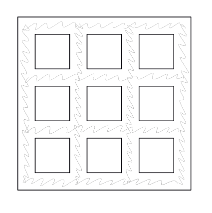
Figure 3:

The corridors $K_{n}$.

The width of these corridors is $3d_{n}$, where $d_{n}=a_{n-1}\varepsilon_{n}$. That is,

$$K_{n}=S_{n}^{+3d_{n}}\setminus\bigcup_{j=0}^{8}\tau_{w_{j}(n)}S_{n-1}\,.$$

To simplify computations, in what follows, we always assume that $\varepsilon_{1}<1$ and that $\varepsilon_{n}\geqslant\varepsilon_{n+1}\geqslant\frac{1}{3}\varepsilon_{n}$. Since

$$\frac{d_{n+1}}{d_{n}}=\frac{3(1+\varepsilon_{n})\varepsilon_{n+1}}{\varepsilon_{n}}\,,$$

these assumptions yield that

$$1<\frac{d_{n+1}}{d_{n}}<6\,.$$

In particular, the sequence $(d_{n})$ is increasing.

6.1.3 Fat systems of squares

We will call the set $E$ fat if $\sum_{n\geqslant 1}\varepsilon_{n}<\infty$. In this case,

$$a_{n}=3^{n}\prod_{j=1}^{n}(1+\varepsilon_{j})=(a+o(1))3^{n}$$

with $a>0$.

Note that since $E_{n}$ consists of $9^{n}$ disjoint translations of the square $S_{0}$, $A(E_{n})=4\cdot 9^{n}$. If the set $E$ is fat then $A(S_{n})=(a^{2}+o(1))9^{n}$, and $A(E_{n})/A(S_{n})=b+o(1)$ with some $b>0$. In particular, fat sets $E$ (and only they) have positive relative area.

6.1.4 Concordance and $\delta$-concordane

Given a ternary system of squares $E$, we call the function $\Phi\colon\mathbb{C}\to\mathbb{C}$ concordant with $E$ if for every $n>k\geqslant 1$ and $0\leqslant j\leqslant 9^{n-k}-1$,

$$\tau_{w_{j}(k,n)}\Phi=\Phi\quad{\rm everywhere\ on\ }S_{k}.$$

Given a sequence $\delta=(\delta_{k})\downarrow 0$, we say that the function $\Phi$ is $\delta$-concordant with $E$ if for every $n>k\geqslant 1$ and $0\leqslant j\leqslant 9^{n-k}-1$,

$$\max_{S_{k}}\bigl{|}\tau_{w_{j}(k,n)}\Phi-\Phi\bigr{|}<\delta_{k}\,.$$

6.2 Main Lemma

For a continuous function $\Phi$ and a compact set $K$, we put

$$M_{\Phi}(K)=\max_{K}|\Phi|,\quad m_{\Phi}(K)=\min_{K}|\Phi|\,.$$

Define the majorant

$$\mathcal{M}_{B}(n)=\exp\Bigl{(}Bn+\pi\sum_{j=1}^{n}\tfrac{1}{\varepsilon_{j}}\Bigr{)},\quad n\geqslant 1$$

with sufficiently large positive $B$ and put $\mathcal{M}_{B}(0)=1$. Then, define the sequence $\Delta$ by

$$\Delta_{n}=\exp\Bigl{(}-\frac{1}{10}\mathcal{M}_{B}(n-1)\Bigr{)},\qquad n\geqslant 1\,.$$

Lemma 5.

For any sufficiently large positive $B$, there exists a non-constant entire function $G$ which is $\Delta$-concordant with $E$, satisfies

$$\log M_{G}\bigl{(}S_{n}\bigr{)}\lesssim e^{-B}\mathcal{M}_{B}(n)\,,$$

and

$$\max_{S_{0}}|G(z)-z|\leqslant\frac{1}{3}\,.$$

We start with the subharmonic counterpart of this lemma.

6.3 Subharmonic construction

Lemma 6.

For any $B\geqslant 20$, there exists a sequence of non-negative subharmonic functions $u_{n}$ in $\mathbb{C}$ with the following properties:

(i) for each $j\in\{0,1,\ldots,8\}$,

$$\tau_{w_{j}(n-1,n)}u_{n-1}=u_{n}\quad\text{on}\ S_{n-1};$$

(ii) $M_{u_{n}}(S_{n}^{+d_{n+1}})<e^{-B+10}\mathcal{M}_{B}(n)$;

(iii) $m_{u_{n}}(K_{n}^{-\frac{1}{2}d_{n}})>\tfrac{1}{2}\,\mathcal{M}_{B}(n-1)$.

Note that by property (i), for every $m>n$, $u_{m}=u_{n}$ everywhere on the square $S_{n}$. Hence, the sequence $(u_{n})$ converges to the limiting subharmonic function $u$. By property (i), the limiting function is concordant with $E$. By (ii), we have $M_{u}(S_{n})\leqslant e^{-B+10}\mathcal{M}_{B}(n)$, $n\geqslant 0$, and by (iii), $m_{u}(K_{n}^{-\frac{1}{2}d_{n}}\bigcap S_{n})\leqslant\tfrac{1}{2}\,\mathcal{M}_{B}(n-1)$, $n\geqslant 1$.

Proof of Lemma 6: Take the subharmonic function

$$h(z)=\begin{cases}\cosh x\cos y\,\ &|y|<\tfrac{\pi}{2},\\ 0\ &\text{otherwise}\,,\end{cases}$$

scale it

$$h_{n}(z)=h\Bigl{(}\frac{\pi}{3d_{n}}z\Bigr{)}\,,$$

$$\xi_{n}=a_{n-1}+\frac{3}{2}d_{n}=a_{n-1}\Bigl{(}1+\frac{3}{2}\varepsilon_{n}\Bigr{)}\,,$$

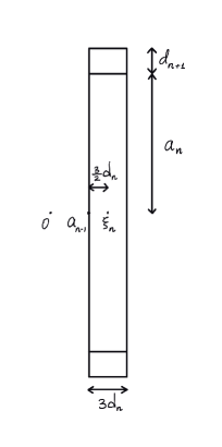
Figure 4:

Scaling, shifting and rotating the function $h$.

and take the upper envelope of $8$ shifted and rotated copies of $h_{n}$:

$$v_{n}(z)=\max\bigl{\{} h_{n}(z+{\rm i}\xi_{n}),h_{n}(z-{\rm i}\xi_{n}),h_{n}({\rm i}(z+\xi_{n})),h_{n}({\rm i}(z-\xi_{n})),$$

$$h_{n}(z+3{\rm i}\xi_{n}),h_{n}(z-3{\rm i}\xi_{n}),h_{n}({\rm i}(z+3\xi_{n})),h_{n}({\rm i}(z-3\xi_{n}))\bigr{\}}\,.$$ (5)

We will need two estimates:

$$m_{v_{n}}\bigl{(}K_{n}^{-\frac{1}{2}d_{n}}\bigr{)}=\cos\Bigl{(}\frac{\pi}{3d_{n}}\cdot d_{n}\Bigr{)}=\frac{1}{2}\,,$$ (6)

and

$$M_{v_{n}}\bigl{(}S_{n}^{+d_{n+1}}\bigr{)} \leqslant\exp\Bigl{(}\frac{\pi}{3d_{n}}\,\bigl{(}a_{n}+d_{n+1}\bigr{)}\Bigr{)}\stackrel{{\scriptstyle d_{n+1}<6d_{n}}}{{<}}\exp\Bigl{(}\frac{\pi}{\varepsilon_{n}}\,\frac{a_{n}}{3a_{n-1}}+2\pi\Bigr{)}$$

$$=\exp\Bigl{(}\frac{\pi}{\varepsilon_{n}}\,(1+\varepsilon_{n})+2\pi\Bigr{)}=\exp\Bigl{(}\frac{\pi}{\varepsilon_{n}}\,+3\pi\Bigr{)}\,.$$ (7)

We put $u_{0}=\tfrac{1}{3}$. Assuming that the subharmonic functions $u_{0},\ldots,u_{n-1}$ have been already defined, we glue together the functions $\tau_{w_{j}(n-1,n)}u_{n-1}$, putting

$$u_{n}=\begin{cases}\max\bigl{\{}\mathcal{M}_{B}(n-1)v_{n},\tau_{w_{j}(n-1,n)}u_{n-1}\bigr{\}}\ &\text{on\ }\tau_{w_{j}(n-1,n)}S_{n-1}^{+\frac{1}{2}d_{n}},\ 0\leqslant j\leqslant 8\,,\\ \mathcal{M}_{B}(n-1)v_{n}\ &\text{otherwise}\,,\end{cases}$$

where $v_{n}$ is the subharmonic function defined in (6.3). Note that this definition ensures property (i) in the statement of the lemma, as

$$v_{n}=0\quad\text{on}\ \bigcup_{j=0}^{8}\tau_{w_{j}(n-1,n)}S_{n-1}\,.$$

We claim that, for $B\geqslant 20$ and $n\geqslant 1$,

$$\max_{\partial(S_{n-1}^{+\frac{1}{2}d_{n}})}u_{n-1}<\mathcal{M}_{B}(n-1)\min_{\partial(S_{n-1}^{+\frac{1}{2}d_{n}})}v_{n}$$

(with $\mathcal{M}_{B}(0)=1$). This claim yields that

$$\tau_{w_{j}(n-1,n)}u_{n-1}<\mathcal{M}_{B}(n-1)v_{n}\quad{\rm on\ }\partial\bigl{(}\tau_{w_{j}(n-1,n)}S_{n-1}^{+\frac{1}{2}d_{n}}\bigr{)},$$

and therefore, the functions $u_{n}$, $n\geqslant 1$, are subharmonic in $\mathbb{C}$.

The case $n=1$ of our claim follows from the lower bound $v_{1}\geqslant\tfrac{1}{2}$ on $\partial(S_{0}^{+\frac{1}{2}d_{1}})$. Now, let $n\geqslant 2$. We know that $u_{n-1}=\mathcal{M}_{B}(n-2)v_{n-1}$ outside the set $\bigcup_{j=0}^{8}\tau_{w_{j}(n-2,n-1)}S_{n-2}^{+\frac{1}{2}d_{n-1}}$. Note that

$$\bigcup_{j=0}^{8}\tau_{w_{j}(n-2,n-1)}S_{n-2}^{+\frac{1}{2}d_{n-1}}\ \subset\ S_{n-1}^{+\frac{1}{2}d_{n-1}}\ \stackrel{{\scriptstyle d_{n-1}<d_{n}}}{{\subset}}\ {\rm interior}\bigl{(}S_{n-1}^{+\frac{1}{2}d_{n}}\bigr{)}.$$

Hence, $u_{n-1}=\mathcal{M}_{B}(n-2)v_{n-1}$ on $\partial\bigl{(}S_{n-1}^{+\frac{1}{2}d_{n}}\bigr{)}$. Furthermore, by the bound (6.3), on $\partial\bigl{(}S_{n-1}^{+\frac{1}{2}d_{n}}\bigr{)}$ we have $\mathcal{M}_{B}(n-2)v_{n-1}<\mathcal{M}_{B}(n-2)\cdot e^{\pi/\varepsilon_{n-1}+3\pi}=e^{-B+3\pi}\mathcal{M}_{B}(n-1)$. For $B\geqslant 20>3\pi+\log 2$, we have $e^{-B+3\pi}<\tfrac{1}{2}$, whence $u_{n-1}<\frac{1}{2}\mathcal{M}_{B}(n-1)$ on $\partial\bigl{(}S_{n-1}^{+\frac{1}{2}d_{n}}\bigr{)}$. On the other hand, $\partial\bigl{(}S_{n-1}^{+\frac{1}{2}d_{n}}\bigr{)}\subset K_{n}^{-\frac{1}{2}d_{n}}$, so applying the lower bound (6) for $v_{n}$, we get the claim.

Note that $u_{n}=\mathcal{M}_{B}(n-1)v_{n}$ on $\partial\bigl{(}S_{n}^{+d_{n+1}}\bigr{)}$, and by (6.3),

$$\mathcal{M}_{B}(n-1)v_{n}<e^{-B+3\pi}\mathcal{M}_{B}(n)$$

therein. This proves (ii). At last, on $K_{n}^{-\frac{1}{2}d_{n}}$, we have

$$u_{n}=\mathcal{M}_{B}(n-1)v_{n}>\tfrac{1}{2}\,\mathcal{M}_{B}(n-1)\,,$$

proving (iii). $\Box$

6.4 Proof of Lemma 5

6.4.1 Beginning the proof

We put $G_{1}(z)=z$ and construct a sequence $(G_{n})$ of entire functions with the following properties:

(i) for $n\geqslant 2$ and $j\in\{0,1,\ldots,8\}$,

$$\max_{S_{n-1}}\bigl{|}G_{n-1}-\tau_{w_{j}(n-1,n)}G_{n}\bigr{|}<\frac{1}{10}\,\Delta_{n}\,,$$

(ii) for $n\geqslant 2$,

$$\log M_{G_{n}}\bigl{(}S_{n}^{+\frac{9}{10}\,d_{n+1}}\bigr{)}<e^{-B+10}\mathcal{M}_{B}(n)\,.$$

Then, the existence of the function $G$ will follow from the following claim.

Claim 1.

For every $1\leqslant k<n$,

$$\max_{S_{k}}\bigl{|}G_{k}-\tau_{w_{j}(k,n)}G_{n}\bigr{|}<\frac{1}{10}\,\sum_{i=k+1}^{n}\Delta_{i}\,.$$

First, assuming that estimates (i) and (ii) and the claim hold, we complete the proof of Lemma 5. On the second step, we prove the claim assuming that the property (i) holds. On the last step, we construct the sequence $(G_{n})$ having properties (i) and (ii).

We put

$$G=G_{1}+\sum_{i\geqslant 2}(G_{i}-G_{i-1})\,.$$

By (i), the series converges locally uniformly in $\mathbb{C}$. Moreover,

$$\max_{S_{k}}|G_{k}-G|\leqslant\frac{1}{10}\,\sum_{i=k+1}\Delta_{i}$$

and then, for $n\geqslant k$,

$$\max_{S_{k}}|G_{n}-G|\leqslant\max_{S_{n}}|G_{n}-G|\leqslant\frac{1}{10}\,\sum_{i=n+1}\Delta_{i}\,.$$

Combining these inequalities with the claim, we conclude that, for every $n>k\geqslant 1$,

$$\max_{S_{k}}|G-\tau_{w_{j}(k,n)}G| \leqslant\Bigl{(}\frac{1}{10}\,\sum_{i=k+1}\Delta_{i}\Bigr{)}+\Bigl{(}\frac{1}{10}\,\sum_{i=n+1}\Delta_{i}\Bigr{)}+\Bigl{(}\frac{1}{10}\,\sum_{i=k+1}\Delta_{i}\Bigr{)}$$

$$<\sum_{j=k+1}\Delta_{i}<\Delta_{k}$$

provided that the parameter $B$ is large enough. That is, the limiting entire function $G$ is $\Delta$-concordant with $E$.

Furthermore, by properties (i) and (ii), the function $G$ satisfies $\log M_{G}(S_{n})\lesssim e^{-B}\mathcal{M}_{B}(n)$ and

$$\max_{S_{0}}|G(z)-z|\leqslant\max_{S_{1}}|G(z)-G_{1}(z)|\leqslant\frac{1}{10}\,\sum_{i\geqslant 2}\Delta_{i}<\frac{1}{3}\,,$$

provided that $B$ is sufficiently large.

6.4.2 Proof of Claim 1

We use induction on $n-k$. The base of induction $n-k=1$ is exactly property (i).

Now, assuming that the claim holds for the pair $(k,n-1)$, we will prove it for $(k,n)$. For every $0\leqslant j\leqslant 9^{n-k}$, we write

$$j=\sum_{\ell=1}^{n-k}j_{\ell}\,9^{\ell-1}\,,$$

and put

$$j^{\prime}=\sum_{\ell=1}^{n-k-1}j_{\ell}\,9^{\ell-1}=j-j_{n-k}\,9^{n-k-1}\,.$$

Then we have

$$\max_{S_{k}}|G_{k}-\tau_{w_{j^{\prime}}(k,n-1)}G_{n-1}|\leqslant\frac{1}{10}\,\sum_{i=k+1}^{n-1}\Delta_{i}\quad(\text{induction\ hypothesis})$$

and

$$\max_{S_{n-1}}|G_{n-1}-\tau_{w_{j_{n-k}}(n-1,n)}G_{n}|\leqslant\frac{1}{10}\,\Delta_{n}\quad(\text{property\ (i)})$$

Then, taking into account that $\tau_{-w_{j^{\prime}}(k,n-1)}S_{k}\subset S_{n-1}$ and using (b), we get

$$\max_{S_{k}}|\tau_{w_{j^{\prime}}(k,n-1)}G_{n-1}-\tau_{w_{j}(k,n)}G_{n}|\,=\,\max_{\tau_{-w_{j^{\prime}}(k,n-1)}S_{k}}|G_{n-1}-\tau_{w_{j_{n-k}}(n-1,n)}G_{n}|$$

$$\leqslant\max_{S_{n-1}}|G_{n-1}-\tau_{w_{j_{n-k}}(n-1,n)}G_{n}|\leqslant\frac{1}{10}\,\Delta_{n}\,.$$

Now, adding (a) and (c), we conclude proof of the claim. $\Box$

Thus, it remains to construct a sequence of entire functions $(G_{n})$ satisfying conditions (i) and (ii).

6.4.3 Constructing the sequence $(G_{n})$

We fix a sequence of smooth cut-off functions $\chi_{n}$, $0\leqslant\chi_{n}\leqslant 1$, so that

$$\chi_{n}=\begin{cases}1\ &\text{on\ }S_{n-1}^{+\frac{3}{5}\,d_{n}}\\ 0\ &\text{on\ }\mathbb{C}\setminus S_{n-1}^{+\frac{4}{5}\,d_{n}}\,.\end{cases}$$

and $\sup_{n}\|\nabla\chi_{n}\|_{\infty}<\infty$ (such a sequence exists since $d_{n}\geqslant d_{1}>0$).

We put $G_{1}(z)=z$ and suppose that the functions $G_{1}$, …, $G_{n-1}$ have already been constructed. We put

$$g_{n}=\sum_{j=0}^{8}\tau_{w_{j}(n-1,n)}\bigl{(}\chi_{n}G_{n-1}\bigr{)}\,,$$

and note that

$$\bar{\partial}g_{n}=\sum_{j=0}^{8}\tau_{w_{j}(n-1,n)}\beta_{n}\,,$$

with $\beta_{n}=G_{n-1}\bar{\partial}\chi_{n}$. Then, we define the function $G_{n}$ by $G_{n}=g_{n}-\alpha_{n}$, where $\alpha_{n}$ is Hörmander’s solution [7, Theorem 4.2.1] to the $\bar{\partial}$-equation $\bar{\partial}\alpha_{n}=\bar{\partial}g_{n}$ satisfying

$$\int_{\mathbb{C}}|\alpha_{n}|^{2}e^{-u_{n}}\,\frac{{\rm d}A}{(1+|z|^{2})^{2}}<\frac{1}{2}\,\int_{\mathbb{C}}|\bar{\partial}g_{n}|^{2}e^{-u_{n}}\,{\rm d}A\,,$$ (8)

where $u_{n}$ are the subharmonic functions constructed in Lemma 6.

6.4.4 Estimating the integral on the RHS of (8)

Note that

$$\operatorname{spt}(\bar{\partial}g_{n}) =\bigcup_{j=0}^{8}\tau_{w_{j}(n-1,n)}\operatorname{spt}(\bar{\partial}\chi_{n})$$

$$\subset\bigcup_{j=0}^{8}\tau_{w_{j}(n-1,n)}\bigl{(}S_{n-1}^{+\frac{4}{5}\,d_{n}}\setminus\text{interior}(S_{n-1}^{+\frac{3}{5}\,d_{n}})\bigr{)}\subset K_{n}^{-\frac{1}{2}d_{n}}\,,$$

and therefore, $u_{n}>\tfrac{1}{2}\,\mathcal{M}_{B}(n-1)$ on $\operatorname{spt}(\bar{\partial}g_{n})$. Furthermore, since $\operatorname{spt}(\bar{\partial}\chi_{n})\subset S_{n-1}^{+\frac{4}{5}d_{n}}$, we have

$$|\bar{\partial}g_{n}|\leqslant C_{\chi}M_{G_{n-1}}(S_{n-1}^{+\frac{9}{10}d_{n}})<C_{\chi}\exp\Bigl{(}e^{-B+10}\mathcal{M}_{B}(n-1)\Bigr{)}$$

with $C_{\chi}=\sup_{n}\|\nabla\chi_{n}\|_{\infty}$ (in the second inequality we have used the inductive assumption). Taking into account that the area of $\operatorname{spt}(\bar{\partial}g_{n})$ is less than $(a_{n}+d_{n})^{2}<(6^{n}+6^{n})^{2}$ and recalling that $u_{n}\geqslant\frac{1}{2}\mathcal{M}_{B}(n-1)$ on $K^{-\frac{1}{2}d_{n}}$, we conclude that the integral on the RHS of (8) does not exceed

$$4\cdot 6^{2n}C_{\chi}^{2}\exp\Bigl{(}\bigl{(}2e^{-B+10}-\frac{1}{2}\bigr{)}\mathcal{M}_{B}(n-1)\Bigr{)}<\exp\Bigl{(}-\frac{2}{5}\mathcal{M}_{B}(n-1)\Bigr{)}\,,$$

provided that the constant $B$ is sufficiently large.

Therefore, by Hörmander’s theorem,

$$\int_{\mathbb{C}}|\alpha_{n}|^{2}e^{-u_{n}}\,\frac{{\rm d}A}{(1+|z|^{2})^{2}}<\frac{1}{2}\,\exp\Bigl{(}-\frac{2}{5}\mathcal{M}_{B}(n-1)\Bigr{)}\,.$$ (9)

6.4.5 Proving property (ii) for the sequence $G_{n}$

Here, we aim to show that

$$\log M_{G_{n}}\bigl{(}S_{n}^{+\frac{9}{10}d_{n+1}}\bigr{)}<e^{-B+10}\,\mathcal{M}_{B}(n)\,.$$

Let $c_{0}<\frac{1}{10}d_{1}$ be a positive constant. Then, for $z\in S_{n}^{+\frac{9}{10}d_{n+1}}$, we have

$$|G_{n}(z)|^{2}\leqslant\frac{1}{\pi c_{0}^{2}}\,\int_{\tau_{z}(c_{0}\mathbb{D})}|G_{n}|^{2}\leqslant\frac{2}{\pi c_{0}^{2}}\,\int_{\tau_{z}(c_{0}\mathbb{D})}(|g_{n}|^{2}+|\alpha_{n}|^{2})\,.$$

To estimate the first integral, we observe that

$$\|g_{n}\|_{\infty}\leqslant\max_{S_{n-1}^{+\frac{4}{5}\,d_{n}}}|G_{n-1}|<\exp\Bigl{(}e^{-B+10}\mathcal{M}_{B}(n-1)\Bigr{)}$$

(in the second inequality we have used the induction assumption). Thus,

$$\frac{2}{\pi c_{0}^{2}}\,\int_{\tau_{z}(c_{0}\mathbb{D})}|g_{n}|^{2}<\frac{1}{2}\,\exp\Bigl{(}2e^{-B+10}\mathcal{M}_{B}(n)\Bigr{)}\,,$$

provided that the constant $B$ is sufficiently large.

To estimate the second integral, using the fact that $z\in S_{n}^{+\frac{9}{10}d_{n+1}}$, we write

$$\int_{\tau_{z}(c_{0}\mathbb{D})}|\alpha_{n}|^{2} <\int_{\mathbb{C}}|\alpha_{n}|^{2}e^{-u_{n}}\,\frac{{\rm d}A}{(1+|z|^{2})^{2}}\cdot C(a_{n}+d_{n+1})^{4}\,\exp\Bigl{(}\max_{S_{n}^{+d_{n+1}}}u_{n}\Bigr{)}$$

$$<C_{1}6^{4n}\,\exp\Bigl{(}-\frac{2}{5}\mathcal{M}_{B}(n-1)+e^{-B+20}\mathcal{M}_{B}(n)\Bigr{)}\,,$$

whence,

$$\frac{2}{\pi c_{0}^{2}}\,\int_{\tau_{z}(c_{0}\mathbb{D})}|\alpha_{n}|^{2}<\frac{1}{2}\exp\Bigl{(}2e^{-B+10}\mathcal{M}_{B}(n)\Bigr{)}\,,$$

again, provided that the constant $B$ is large enough. Thus,

$$|G_{n}|<\exp\Bigl{(}e^{-B+10}\mathcal{M}_{B}(n)\Bigr{)}$$

everywhere on $S_{n}^{+\frac{9}{10}d_{n+1}}$, as we have claimed.

6.4.6 Proving property (i) for the sequence $G_{n}$

First, we note that

$$\max_{S_{n-1}}|G_{n-1}-\tau_{-w_{j}(n-1,n)}G_{n}|=\max_{\tau_{w_{j}(n-1,n)}S_{n-1}}|\alpha_{n}|\,,$$

and that $\alpha_{n}$ is analytic in the $c_{0}$-neighbourhood of each of the sets $\tau_{w_{j}(n-1,n)}S_{n-1}$. Then, for every $j\in\{0,1,\ldots,8\}$ and every $z\in\tau_{w_{j}(n-1,n)}S_{n-1}$, we have

$$|\alpha_{n}(z)|^{2} \leqslant\frac{1}{\pi c_{0}^{2}}\int_{\tau_{z}(c_{0}\mathbb{D})}|\alpha_{n}|^{2}$$

$$<\int_{\mathbb{C}}|\alpha_{n}|^{2}e^{-u_{n}}\,\frac{{\rm d}A}{(1+|z|^{2})^{2}}\cdot C(a_{n}+c_{0})^{4}\exp\Bigl{(}\max_{\tau_{w_{j}(n-1,n)}S_{n-1}^{+c_{0}}}u_{n}\Bigr{)}$$

$$\stackrel{{\scriptstyle\eqref{eq-norm-alpha}}}{{<}}C^{\prime}(a_{n}+c_{0})^{4}\exp\Bigl{(}\,\max_{\tau_{w_{j}(n-1,n)}S_{n-1}^{+c_{0}}}\,u_{n}-\frac{2}{5}\mathcal{M}_{B}(n-1)\Bigr{)}\,.$$

Recall that $u_{n}=\tau_{w_{j}(n-1,n)}u_{n-1}$ on each square $\tau_{w_{j}(n-1,n)}S_{n-1}$. Then, recalling that $d_{n}>1$ and choosing $c_{0}<1$, we see that

$$\max_{\tau_{w_{j}(n-1,n)}S_{n-1}^{+c_{0}}}u_{n}=\max_{S_{n-1}^{+c_{0}}}u_{n-1}\leqslant\max_{S_{n-1}^{+d_{n}}}u_{n-1}<e^{-B+10}\mathcal{M}_{B}(n-1)\,.$$

Therefore,

$$|\alpha_{n}(z)|^{2}\leqslant C_{1}6^{4n}\exp\Bigl{(}-\frac{2}{5}\mathcal{M}_{B}(n-1)+e^{-B+10}\mathcal{M}_{B}(n-1)\Bigr{)}<\frac{1}{100}\,e^{-\frac{1}{5}\,\mathcal{M}_{B}(n-1)}\,,$$

provided that $B$ is sufficiently large, and finally,

$$\max_{\tau_{w_{j}(n-1,n)}S_{n-1}}|\alpha_{n}|<\frac{1}{10}\,e^{-\frac{1}{10}\,\mathcal{M}_{B}(n-1)}=\frac{1}{10}\,\Delta_{n}\,,$$

again, provided that $B$ is sufficiently large. This completes the (somewhat long) proof of Lemma 5. $\Box$

7 A version of the Krylov-Bogolyubov construction

7.1 Some notation

In this section, we denote by $(S_{n})$ any increasing sequence of squares centered at the origin with the side-lengths tending to infinity.

If $S\subset\mathbb{C}$ is a square and $X\subset\mathbb{C}$ is a Borel set, then we denote the relative area of $X$ in $S$ by

$$A_{S}(X)=\frac{A(X\bigcap S)}{A(S)}\,.$$

For an entire function $G\in\mathcal{E}$, let $\mathcal{O}_{G}=\{\tau_{w}G\}_{w\in\mathbb{C}}$ denote its orbit and $\bar{\mathcal{O}}_{G}$ denote the closure of $\mathcal{O}_{G}$ in $\mathcal{E}$.

For a compact set $K\subset\mathbb{C}$ and a continuous function $f\colon K\to\mathbb{R}$, we denote by $\operatorname{osc}_{K}f=\max_{K}f-\min_{K}f$, the oscillation of $f$ on $K$.

7.2 The Lemma

Lemma 7.

Let $G\in\mathcal{E}$.

(i) Suppose that there exists an increasing sequence $(M_{k})\uparrow+\infty$ such that

$$\lim_{k\to\infty}\,\liminf_{n\to\infty}\,A_{S_{n}}\bigl{\{}w\colon\max_{\tau_{w}S_{k}}|G|\leqslant M_{k}\bigr{\}}=1\,,$$ (10)

and there exists a square $S$ and a constant $c>0$ such that

$$\limsup_{n\to\infty}A_{S_{n}}\bigl{\{}w\colon\operatorname{osc}_{\tau_{w}S}|G|\geqslant c\bigr{\}}>0\,.$$ (11)

Then there exists a translation-invariant probability measure $\lambda$ supported by $\bar{\mathcal{O}}_{G}$ which does not charge the constant functions.

(ii) Furthermore, suppose that condition (10) is replaced by a stronger one:

$$\sum_{k\geqslant 1}\Bigl{(}1-\liminf_{n\to\infty}\,A_{S_{n}}\bigl{\{}w\colon\max_{\tau_{w}S_{k}}|G|\leqslant M_{k}\bigr{\}}\Bigr{)}<\infty$$ (12)

and that condition (11) continues to hold. Then, for $\lambda$-a.e. $F\in\mathcal{E}$,

$$\limsup_{k\to\infty}\bigl{(}\max_{S_{k}}|F|-M_{k}\bigr{)}\leqslant 0\,.$$

It is worth mentioning that condition (i) already yields the upper bound though only on a subsequence of the squares $S_{k}$: for $\lambda$-a.e. $F\in\mathcal{E}$,

$$\liminf_{k\to\infty}\bigl{(}\max_{S_{k}}|F|-M_{k}\bigr{)}\leqslant 0\,.$$

7.3 Proof of part (i) of Lemma 7

Consider the sequence of probability measures on $\mathcal{E}$:

$$\lambda_{n}=\frac{1}{A(S_{n})}\,\int_{S_{n}}\delta_{\tau_{w}G}\,{\rm d}A(w)\,.$$

In other words, for any Borel set $\mathcal{X}\subset\mathcal{E}$,

$$\lambda_{n}(\mathcal{X})=\frac{1}{A(S_{n})}\,\int_{S_{n}}{1\hskip-2.5pt{\rm l}}_{\mathcal{X}}(\tau_{w}G)\,{\rm d}A(w)=A_{S_{n}}\bigl{\{}w\colon\tau_{w}G\in\mathcal{X}\bigr{\}}.$$

7.3.1 Tightness of the sequence $(\lambda_{n})$

We claim that $(\lambda_{n})$ is a tight sequence of probability measures, that is, for every $\delta>0$, there exists a compact set $\mathcal{K}\subset\mathcal{E}$ such that, for every $n\geqslant 1$, $\lambda_{n}(\mathcal{K})>1-\delta$.

To see this, given $k\geqslant 2$, we choose $n_{k}>k$ so that for $n\geqslant n_{k}$,

$$A_{S_{n}}\bigl{\{}w\colon\max_{\tau_{w}S_{k}}|G|>M_{n_{k}}\bigr{\}}<\frac{1}{k^{2}}\,,$$

and let

$$\mu_{k}=\max_{2S_{n_{k}-1}}|G|+M_{n_{k}}\,,$$

where $2S_{n_{k}-1}$ is the square concentric with $S_{n_{k}-1}$ and having double the side-length. The sets

$$\mathcal{K}_{\ell}=\bigl{\{}F\in\mathcal{E}\colon\max_{S_{k}}|F|\leqslant\mu_{k}\ {\rm for\ }k\geqslant\ell\bigr{\}}$$

are compact subsets of $\mathcal{E}$. We will show that for any $n\geqslant 1$ and any $\ell\geqslant 2$,

$$\lambda_{n}(\mathcal{K}_{\ell})\geqslant 1-\frac{1}{\ell-1}\,,$$

which yields the tightness of $(\lambda_{n})$. Indeed,

$$\mathcal{E}\setminus\mathcal{K}_{\ell}=\bigcup_{k\geqslant\ell}\mathcal{X}_{k}\,,$$

where $\mathcal{X}_{k}=\bigl{\{}F\in\mathcal{E}\colon\max_{S_{k}}|F|>\mu_{k}\bigr{\}}$, and $\lambda_{n}(\mathcal{X}_{k})=A_{S_{n}}\bigl{\{}w\colon\max_{\tau_{-w}S_{k}}|G|>\mu_{k}\bigr{\}}$. For $1\leqslant n\leqslant n_{k}-1$ and $w\in S_{n}$, we have

$$\max_{\tau_{w}S_{k}}|G|\leqslant\max_{S_{n}+S_{k}}|G|\leqslant\max_{2S_{n_{k}-1}}|G|<\mu_{k}$$

(recall that $k\leqslant n_{k}-1$), whence, for these $n$s, $\bigl{\{}w\colon\max_{\tau_{w}S_{k}}|G|>\mu_{k}\bigr{\}}\bigcap S_{n}=\emptyset$. On the other hand, for $n\geqslant n_{k}$, we have

$$\lambda_{n}(\mathcal{X}_{k})=A_{S_{n}}\bigl{\{}w\colon\max_{\tau_{w}S_{k}}|G|>\mu_{k}\bigr{\}}\leqslant A_{S_{n}}\bigl{\{}w\colon\max_{\tau_{w}S_{k}}|G|>M_{n_{k}}\bigr{\}}<\frac{1}{k^{2}}\,.$$

Thus,

$$\lambda_{n}(\mathcal{E}\setminus\mathcal{K}_{l})\leqslant\sum_{k\geqslant\ell}\lambda_{n}(\mathcal{X}_{\ell})<\sum_{k\geqslant\ell}\frac{1}{k^{2}}<\frac{1}{\ell-1}\,,$$

proving the tightness of $(\lambda_{n})$.

7.3.2 Translation-invariance of the limiting measure

Now, let $\lambda$ be any limiting probability measure for the sequence $(\lambda_{n})$. Since each measure $\lambda_{n}$ is supported by the orbit $\mathcal{O}_{G}$, clearly, $\lambda$ is supported by the closure of the orbit $\bar{\mathcal{O}}_{G}$.

The measure $\lambda$ is translation-invariant. This follows from the fact that for any $n\geqslant 1$, any $\zeta\in\mathbb{C}$, and any Borel set $\mathcal{X}\subset\mathcal{E}$,

$$\bigl{|}\lambda_{n}(\tau_{\zeta}\mathcal{X})-\lambda_{n}(\mathcal{X})\bigr{|}\leqslant\frac{A(S_{n}\triangle\tau_{\zeta}S_{n})}{A(S_{n})}\leqslant\frac{O(|\zeta|)}{L(S_{n})}\,,$$

where $\triangle$ denotes the symmetric difference of sets, and $L(S_{n})$ is the side-length of $S_{n}$.

7.3.3 A modification of the limiting measure does not charge the constant functions

At last, we can specify the measure $\lambda$ such that it will not charge the set $\{\rm const\}$ of constant functions. Indeed, following our assumption (11) and passing if necessary to some subsequence, we may assume that a positive limit exists

$$\lim_{n\to\infty}A_{S_{n}}\bigl{\{}w\colon\operatorname{osc}_{\tau_{w}S}|G|>c\bigr{\}}=\alpha>0\,.$$

This yields that $\lambda(\mathcal{E}\setminus\{{\rm const}\})\geqslant\alpha>0$. To see this, let $U=\{F\in\mathcal{E}\colon\operatorname{osc}_{S}|F|<\frac{1}{2}\,c\}$. Then $U$ is an open set and $U\supset\{\text{const}\}$. Hence, it is enough to show that, for each $n$, $\lambda_{n}(U)\leqslant 1-\alpha$. This holds since

$$\lambda_{n}(U)=A_{S_{n}}\bigl{(}\bigl{\{}w\colon\tau_{w}G\in U\bigr{\}}\bigl{)}=A_{S_{n}}\bigl{(}\bigl{\{}w\colon\operatorname{osc}_{S}\tau_{w}G<\frac{c}{2}\bigr{\}}\bigr{)}\\ =A_{S_{n}}\bigl{(}\bigl{\{}w\colon\operatorname{osc}_{\tau_{w}S}G<\frac{c}{2}\bigr{\}}\bigr{)}\leqslant 1-\alpha\,.$$

Then, if needed, we replace $\lambda$ by its restriction on $\mathcal{E}\setminus\{{\rm const}\}$ and normalize it to make $\lambda$ the probability measure. This completes the proof of part (i). $\Box$

7.4 Proof of part (ii) of Lemma 7

Now, we suppose that condition (12) holds, and assume that the probability measures $(\lambda_{n})$ and $\lambda$ are the same as in the proof of part (i). Consider the open set

$$\mathcal{X}_{k}=\bigl{\{}F\in\mathcal{E}\colon\max_{S_{k}}|F|>M_{k}\bigr{\}}\,.$$

We have

$$\lambda_{n}(\mathcal{X}_{k})=A_{S_{n}}\bigl{(}\bigl{\{}w\colon\max_{\tau_{w}S_{k}}|G|>M_{k}\bigr{\}}\bigr{)}\,,$$

whence, by (12),

$$\sum_{k\geqslant 1}\Bigl{(}\limsup_{n\to\infty}\lambda_{n}(\mathcal{X}_{k})\Bigr{)}<\infty\,.$$

Furthermore, since the sets $\mathcal{X}_{k}$ are open,

$$\lambda(\mathcal{X}_{k})\leqslant\limsup_{n\to\infty}\lambda_{n}(\mathcal{X}_{k})\,,$$

so

$$\sum_{k\geqslant 1}\lambda(\mathcal{X}_{k})<\infty\,.$$

Hence, applying the Borel-Cantelli lemma, we conclude that

$$\lambda\Bigl{(}\bigcap_{\ell\geqslant 1}\bigcup_{k\geqslant\ell}\mathcal{X}_{k}\Bigr{)}=0\,,$$

which means that $\lambda$-a.e. $F\in\mathcal{E}$ does not belong to any $\mathcal{X}_{k}$ with $k\geqslant k_{0}(F)$, i.e.,

$$\limsup_{k\to\infty}\bigl{(}\max_{S_{k}}|F|-M_{k}\bigr{)}\leqslant 0\,.$$

This proves part (ii) and finishes off the proof of Lemma 7. $\Box$

8 Proof of Theorems 1B, 2B, and 3B

After the work we have done in Lemmas 5 and 7, the proofs of these theorems is rather straightforward.

8.1 Proof of Theorem 1B

We take the sequence

$$\varepsilon_{j}=\frac{1}{(j+10)\log^{3}(j+10)},\quad j\geqslant 1\,,$$

put $a_{0}=1$ and $a_{n}=3(1+\varepsilon_{j})a_{n-1}$ for $n\geqslant 1$, and (with some conflict of notation used in Lemma 6) $S_{n}^{\prime}=[-a_{n},a_{n}]^{2}$. By $G$ we denote the corresponding entire function with properties as in Lemma 5. We fix a sufficiently large value of the parameter $B$ as in Lemma 5 and then will drop dependence on $B$ from our notation. We claim that

• conditions (12) and (11) of Lemma 7 (part (ii)) are hold for the sequences $S_{n}=S_{2^{n}}^{\prime}$ and $M_{n}=\exp\mathcal{M}(2^{n+1})+1$.

8.1.1

First, we verify convergence of the series

$$\sum_{k\geqslant 1}\Bigl{(}\limsup_{n\to\infty}A_{S_{n}}\bigl{\{}w\colon\max_{\tau_{w}S_{k}}|G|>M_{k}\bigr{\}}\Bigr{)}<\infty\,.$$

For this, we need to bound the relative area

$$A_{S_{2^{n}}^{\prime}}\bigl{(}\bigl{\{}w\colon\max_{\tau_{w}S_{2^{k}}^{\prime}}|G|>\exp\mathcal{M}(2^{k+1})+1\bigr{\}}\bigr{)}\,.$$

We note that for $\zeta\in[-a_{2^{k+1}}+a_{2^{k}},a_{2^{k+1}}-a_{2^{k}}]^{2}$, the translations $\tau_{\zeta}S_{2^{k}}^{\prime}$ belong to $S_{2^{k+1}}^{\prime}$. Thus, for $w=w_{j}(2^{k+1},2^{n})+\zeta$, $0\leqslant j\leqslant 9^{2^{n}-2^{k+1}}-1$, we have

$$\max_{\tau_{w}S_{2^{k}}^{\prime}}|G| =\max_{\tau_{\zeta}S_{2^{k}}^{\prime}}|\tau_{-w_{j}(2^{k+1},2^{n})}G|$$

$$\leqslant\max_{S_{2^{k+1}}^{\prime}}|\tau_{-w_{j}(2^{k+1},2^{n})}G|$$

$$<\max_{S_{2^{k+1}}^{\prime}}|G|+\Delta_{2^{k+1}}$$

$$<M_{k}\,.$$

The relative area of the set of these $w$s in $S_{2^{n}}^{\prime}$ is

$$\frac{9^{2^{n}-2^{k+1}}(a_{2^{k+1}}-a_{2^{k}})^{2}}{a_{2^{n}}^{2}} =\frac{9^{2^{n}-2^{k+1}}(a_{2^{k+1}}-a_{2^{k}})^{2}}{9^{2^{n}-2^{k+1}}a_{2^{k+1}}^{2}\prod_{j=2^{k+1}}^{2^{n}}(1+\varepsilon_{j})^{2}}\qquad({\rm since\ }a_{n}=3a_{n-1}(1+\varepsilon_{n}))$$

$$=\Bigl{(}1-\frac{a_{2^{k}}}{a_{2^{k+1}}}\Bigr{)}^{2}\cdot\Bigl{(}1-(2+o(1))\sum_{j=2^{k+1}}^{2^{n}}\varepsilon_{j}\Bigr{)}$$

$$\geqslant 1-2\,\frac{a_{2^{k}}}{a_{2^{k+1}}}-(2+o(1))\sum_{j\geqslant 2^{k+1}}\varepsilon_{j}\,,\qquad k\to\infty\,.$$

Hence,

$$\limsup_{n\to\infty}A_{S_{n}}\bigl{\{}w\colon\max_{\tau_{w}S_{k}}|G|>M_{k}\bigr{\}}\leqslant 2\,\frac{a_{2^{k}}}{a_{2^{k+1}}}+(2+o(1))\sum_{j\geqslant 2^{k+1}}\varepsilon_{j}\,.$$ (13)

At last, for $\ell\to\infty$, $a_{\ell}=(a+o(1))3^{\ell}$ with some $a>0$, and

$$\sum_{j\geqslant\ell}\varepsilon_{j}=\frac{1+o(1)}{2\log^{2}\ell}\qquad(\,{\rm since\ }\varepsilon_{j}=\frac{1}{(j+10)\log^{3}(j+10)}\,)\,.$$

Therefore, the RHS of (13) is

$$\lesssim 3^{-2^{k}}+\frac{1}{k^{2}}\,,$$

which is what we need for condition (12).

8.1.2

To verify condition (11), we take $S=[-a_{1},a_{1}]^{2}$, $\delta<a_{1}-1$, and note that for $w=w_{j}(1,2^{n})+\zeta$ with $0\leqslant j\leqslant 9^{2^{n}-1}-1$, $|\zeta|<\delta$, we have $\tau_{w}S\supset\tau_{w_{j}(1,2^{n})}[-1,1]^{2}$. Therefore,

$$\operatorname{osc}_{\tau_{w}S}|G| \geqslant\operatorname{osc}_{\tau_{w_{j}(1,2^{n})}[-1,1]^{2}}|G|$$

$$\geqslant\operatorname{osc}_{[-1,1]^{2}}|G|-\Delta_{1}$$

$$\geqslant\operatorname{osc}_{[-1,1]^{2}}|z|-\frac{1}{3}-\Delta_{1}$$

$$\geqslant c>0$$

since $\frac{1}{3}+\Delta_{1}<\frac{1}{3}+1<\sqrt{2}=\operatorname{osc}_{[-1,1]^{2}}|z|$. Thus, the set $\bigl{\{}w\colon\operatorname{osc}_{\tau_{w}S}|G|>c\bigr{\}}$ contains the $\delta$-neighbourhood of the set $\bigl{\{}w_{j}(1,2^{n})\colon 0\leqslant j\leqslant 9^{2^{n}-1}-1\bigr{\}}$. Hence, the relative area of this set in $S_{n}=S_{2^{n}}^{\prime}$ is bounded from below by

$$\frac{9^{2^{n}}\pi\delta^{2}}{a_{2^{n}}^{2}}\gtrsim\delta^{2}>0\,,$$

which yields condition (11).

8.1.3

At last, applying Lemma 7, we see that for $\lambda$-a.e. $F\in\mathcal{E}$,

$$\limsup_{[-a_{2^{n}},a_{2^{n}}]^{2}}\bigl{(}|F|-\exp\mathcal{M}(2^{n+1})\bigr{)}\leqslant 1\,.$$

In our case $\mathcal{M}(m)\lesssim\exp(Cm^{2}\log^{3}m)$, whence $\mathcal{M}(2^{n+1})\leqslant\exp(C2^{2n}n^{3})$. Then, given $R\geqslant 10$, we choose $n$ such that $a_{2^{n-1}}<R\leqslant a_{2^{n}}$ and get

$$\log M_{F}(R)=\max_{R\,\mathbb{D}}\log|F|\leqslant\max_{[-a_{2^{n}},a_{2^{n}}]^{2}}\log|F|\leqslant\exp(C2^{2n}n^{3})\,.$$

Furthermore, recalling that $a_{m}=(a+o(1))3^{m}$, we see that $2^{n}\lesssim\log a_{2^{n-1}}$, whence $2^{2n}n^{3}\lesssim(\log R)^{2}(\log\log R)^{3}$, proving Theorem 1B. $\Box$

8.2 Proof of Theorem 2B

Here, we take $\varepsilon_{j}=3^{-j}$, and let $G$ be the entire function constructed by using Lemma 5. Note that in this case

$$\mathcal{M}(n)\leqslant\exp\bigl{(}C3^{n}\bigr{)}\leqslant\exp\bigl{(}Ca_{n}\bigr{)}\,.$$

Given $R\geqslant 10$ we choose $n$ so that $a_{n-1}<R\leqslant a_{n}$ and get

$$\log M_{G}(R)\leqslant e^{CR}\,.$$

Furthermore, given a square $S_{k}$, for any $n>k$ and any $j\in\bigl{\{}0,1,\ldots,9^{n-k}-1\bigr{\}}$, we have

$$\max_{S_{k}}\bigl{|}\tau_{w_{j}(k,n)}G-G\bigr{|}<\Delta_{k}\,.$$

Given $\varepsilon>0$ and a compact set $K\subset\mathbb{C}$, we choose $k$ so large that $K\subset S_{k}$ and

$$\max_{S_{k}}\bigl{|}\tau_{w_{j}(k,n)}G-G\bigr{|}<\varepsilon\qquad{\rm for\ any\ }n>k\,.$$

Observing that each square $S\subset\mathbb{C}$ with the side length $C3^{k+1}$ contains at least one point of the set

$$\bigl{\{}w_{j}(k,n)\colon 0\leqslant j\leqslant 9^{n-k}-1,n\geqslant k+1\bigr{\}}\,,$$

we complete the proof of Theorem 2B. $\Box$

8.3 Proof of Theorem 3B

As in the proof of Theorem 2B, we take $\varepsilon_{j}=3^{-j}$. We denote by $(S_{n})$ the corresponding ternary system of squares and let $G$ be the entire function as in Lemma 5. We fix $B$ so large that

$$\max_{S_{k}}|G|+\sum_{j\geqslant 1}\Delta_{j}<e^{\mathcal{M}_{B}(k)}\,,$$

and drop the parameter $B$ in our notation. As in the proof of Theorem 1B, a straightforward verification, which we skip, shows that conditions (10) and (11) of Lemma 7 are satisfied.

As before, we put

$$\lambda_{n}=\frac{1}{A(S_{n})}\,\int_{S_{n}}\delta_{\tau_{w}G}\,{\rm d}A(w)\,,$$

denote by $\lambda$ any limiting measure and by $(n_{i})$ the sequence of indices such that $\lambda_{n_{i}}\to\lambda$ weakly.

We fix $t$ sufficiently large and choose $k$ so that $e^{\mathcal{M}(k-1)}<t\leqslant e^{\mathcal{M}(k)}$. Then for all $t$’s (except maybe a countable set of values which we may neglect),

$$\lambda\bigl{\{}F\in\mathcal{E}\colon|F(0)|>t\bigr{\}} =\lim_{i\to\infty}\lambda_{n_{i}}\bigl{\{}F\in\mathcal{E}\colon|F(0)|>t\bigr{\}}$$

$$=\lim_{i\to\infty}A_{S_{n_{i}}}\bigl{\{}w\colon|G(w)|>t\bigr{\}}\,.$$

Since $t>e^{\mathcal{M}(k-1)}$, we have $|G|<t$ on $S_{k-1}$, as well as on all translations $\tau_{w_{j}(k-1,n)}S_{k-1}$. Thus,

$$A_{S_{n}}\bigl{\{}w\colon|G(w)|>t\bigr{\}} \leqslant A_{S_{n}}\Bigl{(}\bigl{(}\bigcup_{j=0}^{9^{n-k}-1}\tau_{w_{j}(k-1,n)}S_{k-1}\bigr{)}^{c}\Bigr{)}$$

$$=1-\frac{9^{n-k}(2a_{k-1})^{2}}{(2a_{n})^{2}}$$

$$=1-\prod_{j=k}^{n}(1+2\varepsilon_{j})^{-2}$$

$$=(2+o(1))\,\sum_{j=k}^{n}\varepsilon_{j}$$

$$\lesssim 3^{-k}\,.$$

On the other hand, we have

$$\log t\leqslant\mathcal{M}(k)\leqslant e^{C3^{k}}\,,$$

whence

$$3^{-k}\lesssim\frac{1}{\log\log t}\,,$$

completing the proof of Theorem 3B. $\Box$

L.B.: School of Mathematics, Tel Aviv University, Tel Aviv, 69978 Israel,
levbuh@post.tau.ac.il

A.G.: School of Mathematics, Tel Aviv University, Tel Aviv, 69978 Israel,
adiglucksam@gmail.com

A.L.: School of Mathematics, Tel Aviv University, Tel Aviv, 69978 Israel,
& Chebyshev Laboratory, St. Petersburg State University, 14th Line V.O., 29B,
Saint Petersburg 199178 Russia, log239@yandex.ru

M.S.: School of Mathematics, Tel Aviv University, Tel Aviv, 69978 Israel,
sodin@post.tau.ac.il

References

- [1] M. E. Becker, Multiparameter groups of measure-preserving tranformations: a simple proof of Wiener’s ergodic theorem. Ann. Prob. 9 (1981), 504–509.
- [2] T. Carleman, Extension d’un théorème de Liouville, Acta Math. 48 (1926), 363–366.
- [3] Y. Domar, On the existence of a largest subharmonic minorant of a given function. Ark. Mat. 3 (1957), 429–440.
- [4] Y. Domar, Uniform boundedness in families related to subharmonic functions. J. London Math. Soc. (2) 38 (1988), 485–491.
- [5] M. Einsiedler, Th. Ward, Ergodic theory with a view towards number theory. Graduate Texts in Mathematics, 259. Springer-Verlag, London, 2011.
- [6] A. A. Goldberg, I. V. Ostrovskii, Value distribution of meromorphic functions. With an appendix by A. Eremenko and J. K. Langley. American Mathematical Society, Providence, RI, 2008.
- [7] L. Hormander, Notions of convexity. Birkhäuser, Boston, MA, 2007.
- [8] B. Tsirelson, Divergence of a stationary random vector field can be always positive (a Weiss’ phenomenon), arXiv:0709.1270
- [9] B. Weiss, Measurable entire functions. The heritage of P. L. Chebyshev: a Festschrift in honor of the 70th birthday of T. J. Rivlin. Ann. Numer. Math. 4 (1997), 599–605.
L.B.:
School of Mathematics, Tel Aviv University, Tel Aviv, 69978 Israel,