Universality in numerical computation with random data. Case studies, analytic results and some speculations.

Percy Deift
Courant Institute
The work in this paper was supported in part by DMS Grant #13000965 (P.D.) and DMS Grant #1303018 (T.T.). Thomas Trogdon^∗
University of California, Irvine

Abstract

We discuss various universality aspects of numerical computations using standard algorithms. These aspects include empirical observations and rigorous results. We also make various speculations about computation in a broader sense.

Acknowledgements.

One of the authors (P.D.) would like to thank the organizers for the invitation to participate in the Abel Symposium 2016 “Computation and Combinatorics in Dynamics, Stochastics and Control”. During the symposium he gave a talk on a condensed version of the paper below.

There are two natural “integrabilities” associated with matrices $M$ . The first concerns random matrix theory where key statistics, such as the distribution of the largest eigenvalue of $M$ , or the gap probability, i.e., the probability that the spectrum of $M$ contains a prescribed gap, are described in an appropriate scaling limit as $N=\dim M\to\infty$ , by the solution of completely integrable Hamiltonian systems, viz., Painlevé equations (see e.g. [Meh]). The second concerns the numerical computation of the eigenvalues of a matrix. Standard eigenvalue algorithms work in the following way. Let $\Sigma_{N}$ denote the set of real $N\times N$ symmetric matrices and let $M\in\Sigma_{N}$ be a given matrix whose eigenvalues one wants to compute. Associated with each algorithm $\mathcal{A}$ , there is, in the discrete case, a map $\varphi=\varphi_{\mathcal{A}}:\Sigma_{N}\to\Sigma_{N}$ , with the properties

•

(isospectral) $\text{spec}\left(\varphi_{\mathcal{A}}(H)\right)=\text{spec}\;(H),\qquad H\in\Sigma_{N}$ ,
•

(convergence) the iterates $X_{k+1}=\varphi_{\mathcal{A}}(X_{k}),\quad k\geq 0,\qquad X_{0}=M$ , converge to a diagonal matrix $X_{\infty},\quad X_{k}\to X_{\infty}$ , as $k\to\infty$ ,

and in the continuum case, there is a flow $t\to X(t)\in\Sigma_{N}$ with the properties

•

(isospectral) $\quad\text{spec}\left(X(t)\right)=\text{spec}\,\left(X(0)\right)$ ,
•

(convergence) the flow $X(t)$ , $t\geq 0$ , $X(0)=M$ , converges to a diagonal matrix $X_{\infty}$ , $X(t)\to X_{\infty}$ as $t\to\infty$ .

In both case, necessarily the (diagonal) entries of $X_{\infty}$ are the eigenvalues of the given matrix $M$ . Now the fact of the matter is that, in most cases of interest, the flow $t\to X(t)$ is Hamiltonian and completely integrable in the sense of Liouville, and in the discrete case we have a “stroboscope theorem”, i.e. there exists a completely integrable Hamiltonian flow $t\to\tilde{X}(t)$ which coincides with the above iterates $X_{k}$ at integer times, $\tilde{X}(k)=X_{k},\;\;k\geq 0$ (see, in particular, [Sym], [DNT], [DLNT]). The abstract QR algorithm is a prime example of such a discrete algorithm, while the Toda algorithm is an example of the continuous case.

Question: What happens if one tries to “marry” these two integrabilities? In particular, what happens when one computes the eigenvalues of a random matrix? In response to this question, the authors in [PDM] initiated a statistical study of the performance of various standard algorithms to compute the eigenvalues of random matrices $M$ from $\Sigma_{N}$ .

Given $\epsilon>0$ , it follows, in the discrete case, that for some $m$ the off-diagonal entries of $X_{m}$ are $O(\epsilon)$ and hence the diagonal entries of $X_{m}$ give the eigenvalues of $X_{0}=M$ to $O(\epsilon)$ . The situation is similar for continuous algorithms $t\to X(t)$ . Rather than running the algorithm until all the off-diagonal entries are $O(\epsilon)$ , it is customary to run the algorithm with deflations as follows. For an $N\times N$ matrix $Y$ in block from

Y=\left[\begin{matrix}Y_{11}&Y_{12}\\ Y_{21}&Y_{22}\end{matrix}\right]

with $Y_{11}$ of size $k\times k$ and $Y_{22}$ of size $(N-k)\times(N-k)$ for some $k\in\left\{1,2,\dots,N-1\right\}$ , the process of projecting $Y\to\text{diag}\;\left(Y_{11},Y_{22}\right)$ is called deflation. For a given $\epsilon>0$ , algorithm $\mathcal{A}$ and matrix $M\in\Sigma_{N}$ , define the $k$ -deflation time $T^{(k)}(M)=T^{(k)}_{\epsilon,\mathcal{A}}(M),\quad 1\leq k\leq N-1$ , to be the smallest value of $m$ such that $X_{m}$ , the $m^{th}$ iterate of algorithm $\mathcal{A}$ with $X_{0}=M$ , has block form

X_{m}=\left[\begin{matrix}X^{(k)}_{11}&X^{(k)}_{12}\\ X^{(k)}_{21}&X^{(k)}_{22}\end{matrix}\right]

with $X^{(k)}_{11}$ of size $k\times k$ and $X^{(k)}_{22}$ of size $(N-k)\times(N-k)$ and $\|X^{(k)}_{12}\|=\|X^{(k)}_{21}\|\leq\epsilon$ . The deflation time $T(M)$ is then defined as

T(M)=T_{\epsilon,\mathcal{A}}(M)=\min_{1\leq k\leq N-1}\quad T^{(k)}_{\epsilon,\mathcal{A}}(M).

If $\hat{k}\in\left\{1,\dots,N-1\right\}$ is such that $T(M)=T^{(\hat{k})}_{\epsilon,\mathcal{A}}(M)$ , it follows that the eigenvalues of $M=X_{0}$ are given by the eigenvalues of the block-diagonal matrix $\text{diag}\left(X^{(\hat{k})}_{11},X^{(\hat{k})}_{22}\right)$ to $O(\epsilon)$ . After running the algorithm to time $T_{\epsilon,\mathcal{A}}(M)$ , the algorithm restarts by applying the basic algorithm $\mathcal{A}$ separately to the smaller matrices $X^{(\hat{k})}_{11}$ and $X^{(\hat{k})}_{22}$ until the next deflation time, and so on. There are again similar considerations for continuous algorithms.

As the algorithm proceeds, the number of matrices after each deflation doubles. This is counterbalanced by the fact that the matrices are smaller and smaller in size, and the calculations are clearly parallelizable. Allowing for parallel computation, the number of deflations to compute all the eigenvalues of a given matrix $M$ to an accuracy $\epsilon$ , will vary from $O(\log N)$ to $O(N)$ .

In [PDM] the authors considered the deflation time $T=T_{\epsilon,\mathcal{A}}=T_{\epsilon,\mathcal{A},\mathcal{E}}$ for $N\times N$ matrices chosen from an ensemble $\mathcal{E}$ . For a given $\epsilon>0$ , algorithm $\mathcal{A}$ and ensemble $\mathcal{E}$ , the authors computed $T(M)$ for 5,000–10,000 samples of matrices $M$ chosen from $\mathcal{E}$ , and recorded the normalized deflation time

(1)

\tilde{T}(M)\equiv\frac{T(M)-\langle T\rangle}{\sigma}

where $\langle T\rangle$ and $\sigma^{2}=\left\langle\left(T-\langle T\rangle\right)^{2}\right\rangle$ are the sample average and sample variance of $T(M)$ , respectively. What the authors found, surprisingly, was that for the given algorithm $\mathcal{A}$ , and $\epsilon$ and $N$ in a suitable scaling range with $N\to\infty$ , the histogram of $\tilde{T}$ was universal, independent of the ensemble $\mathcal{E}$ . In other words, the fluctuations in the deflation time $\tilde{T}$ , suitably scaled, were universal, independent of $\mathcal{E}$ . Figure 1 displays some of the numerical results from [PDM].

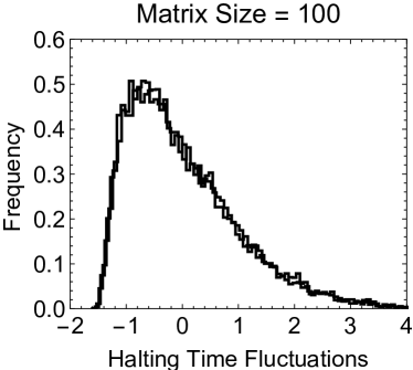
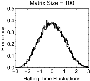
Refer to caption — Figure 1: Universality for $\tilde{T}$ when (a) $\mathcal{A}$ is the QR eigenvalue algorithm and when (b) $\mathcal{A}$ is the Toda algorithm. Panel (a) displays the overlay of two histograms for $\tilde{T}$ in the case of QR, one for each of the two ensembles $\mathcal{E}=\mathrm{BE}$ , consisting of iid mean-zero Bernoulli random variables and $\mathcal{E}=\mathrm{GOE}$ , consisting of iid mean-zero normal random variables. Here $\epsilon=10^{-10}$ and $N=100$ . Panel (b) displays the overlay of two histograms for $\tilde{T}$ in the case of the Toda algorithm, and again $\mathcal{E}=\mathrm{BE}$ or $\mathrm{GOE}$ . And here $\epsilon=10^{-8}$ and $N=100$ .

Figure 1(a) displays data for the QR algorithm, which is discrete, and Figure 1(b) displays data for the Toda algorithm, which is continuous. Note that the histograms in Figures 1(a) and 1(b) are very different: Universality is observed with respect to the ensembles $\mathcal{E}$ —not with respect to the algorithms $\mathcal{A}$ .

Subsequently in [DMOT] the authors raised the question of whether the universality results in [PDM] were limited to eigenvalue algorithms for real symmetric matrices, or whether they were present more generally in numerical computation. And indeed the authors in [DMOT] found similar universality results for a wide variety of numerical algorithms, including

(a)

other algorithms such as the QR algorithm with shifts¹¹1The QR algorithm with shifts is the accelerated version of the QR algorithm that is used in practice., the Jacobi eigenvalue algorithm, and also algorithms applied to complex Hermitian ensembles
(b)

the conjugate gradient and GMRES algorithms to solve linear $N\times N$ systems $Hx=b$ with $H$ and $b$ random
(c)

an iterative algorithm to solve the Dirichlet problem $\Delta u=0$ in a random star-shaped region $\Omega\subset\mathbb{R}^{2}$ with random boundary data $f$ on $\partial\Omega$
(d)

a genetic algorithm to compute the equilibrium measure for orthogonal polynomials on the line.

In [DMOT] the authors also discuss similar universality results obtained by Bakhtin and Correll [BC] in a series of experiments with live participants recording

(e)

decision making times for a specified task.

Whereas (a) and (b) concern finite dimensional problems, (c) shows that universality is also present in problems that are genuinely infinite dimensional. And whereas (a), (b) and (c) concern, in effect, deterministic dynamical systems acting on random initial data, problem (d) shows that universality is also present in genuinely stochastic algorithms.

The demonstration of universality in problems (a)–(d) raises the following issue: Given the common view of neuroscientists that the brain is just a big computer with hardware and software, one should be able to find evidence of universality in some neural computations. It is this issue that led the authors in [DMOT] to the work of Bakhtin and Correll. In [BC] each of the participants is shown a large number $k$ of diagrams and then asked to make a decision about a particular geometric feature of each diagram. What is then recorded is the time it takes for the participant to reach his’r decision. Thus each participant produces $k$ decision times $t$ which are then centered and scaled as in (1) to obtain a normalized decision time

(2)

\tilde{t}=\frac{t-\langle t\rangle}{\sigma}.

The distribution of $\tilde{t}$ is then recorded in a histogram. Each of the participants produces such a histogram, and what is remarkable is that the histograms are, with a few exceptions, (essentially) the same. Furthermore, in [BC], Bakhtin and Correll developed a Curie-Weiss-type statistical mechanical model for the decision process, and obtained a distribution function $f_{BC}$ which agrees remarkably well with the (common) histogram obtained by the participants. We note that the model of Bakhtin and Correll involves a particular parameter, the spin flip intensity $c_{i}$ . In [BC] the authors made one particular choice for $c_{i}$ . However, as shown in [DMOT], if one makes various other choices for $c_{i}$ , then one still obtains the same distribution $f_{BC}$ . In other words, the Bakhtin-Correll model itself has an intrinsic universality. In an independent development Sagun, Trogdon and LeCun [STL] considered, amongst other things, search times on Google^TM for a large number of words in English and in Turkish. They then centered and scaled these times as in (1), (2) to obtain two histograms for normalized search times, one for English words and one for Turkish words. To their great surprise, both histograms were the same and, moreover, extremely well described by $f_{BC}$ . So we are left to ponder the following puzzlement: Whatever the neural stochastics of the participants in the study in [BC], and whatever the stochastics in the Curie-Weiss model, and whatever the mechanism in Google^TM’s search engine, a commonality is present in all three cases expressed through the single distribution function $f_{BC}$ .

All of the above results are numerical. In order to establish universality as a bona fide phenomenon in numerical analysis, and not just an artifact, suggested, however strongly, by certain computations as above, P. Deift and T. Trogdon in [DT1] considered the Toda eigenvalue algorithm mentioned above. In place of the deflation time $T(M)=\min_{1\leq k\leq N-1}\;\;T^{(k)}_{\epsilon\,\mathcal{A}}(M)$ , $\mathcal{A}=\text{Toda algorithm}$ , Deift and Trogdon used the 1-deflation time $T^{(1)}(M)=T^{(1)}_{\epsilon,\mathcal{A}}(M)$ as the stopping time for the algorithm. In other words, given $\epsilon>0$ and an ensemble $\mathcal{E}$ , they ran the Toda algorithm $t\to X(t)$ with $X(0)=M\in\mathcal{E}$ , until a time $t$ where

t=T^{(1)}(M)=\inf\left\{s\geq 0:\sum^{N}_{j=2}\left(X_{1j}(s)\right)^{2}\leq\epsilon^{2}\right\}.

It follows by perturbation theory that $\left|X_{11}\left(T^{(1)}(M)\right)-\lambda_{j^{\ast}}(M)\right|\leq\epsilon$ for some eigenvalue $\lambda_{j^{\ast}}(M)$ of $M$ . But the Toda algorithm is known to be ordering, i.e. $X(t)\to X_{\infty}=\text{diag}\left(\lambda_{1}(M),\lambda_{2}(M),\dots\lambda_{N}(M)\right)$ , where the eigenvalues of $M$ are ordered, $\lambda_{1}(M)\geq\lambda_{2}(M)\geq\dots\geq\lambda_{N}(M)$ . It follows then that (for $\epsilon$ sufficiently small and $T^{(0)}_{\epsilon,\mathcal{A}}$ correspondingly large) $j^{\ast}=1$ so that the Toda algorithm with stopping time $T^{(1)}=T^{(1)}_{\epsilon,\mathcal{A}}$ computes the largest eigenvalue of $M$ to accuracy $\epsilon$ with high probability.

The main result in [DT1] is the following. For invariant and generalized Wigner random matrix ensembles²²2See Appendix A in [DT1] for a precise description of the matrix ensembles considered in Theorem 1. there is an ensemble dependent constant $c_{\mathcal{E}}$ such that the following limit exists (see [PS] and [WBF])

(3)

F^{\text{gap}}_{\beta}(t)=\lim_{N\to\infty}\operatorname{Prob}\left(\frac{1}{c^{2/3}_{\mathcal{E}}\;2^{-2/3}\;N^{2/3}\left(\lambda_{1}-\lambda_{2}\right)}\leq t\right),\qquad t\geq 0.

Here $\beta=1$ for the real symmetric case, $\beta=2$ for the complex Hermitian case. Thus $F^{\text{gap}}_{\beta}(t)$ is the distribution function for the (inverse of the) gap $\lambda_{1}-\lambda_{2}$ between the largest two eigenvalues of $M$ , on the appropriate scale as $N\to\infty$ .

Theorem 1 (Universality for $T^{(1)}$ ).

Let $0<\sigma<1$ be fixed and let $(\epsilon,N)$ be in the scaling region

(4)

\frac{\log\epsilon^{-1}}{\log N}\geq\frac{5}{3}+\frac{\sigma}{2}\ .

Then if $M$ is distributed according to any real $(\beta=1$ ) or complex $(\beta=2)$ invariant or Wigner ensemble, we have

(5)

\lim_{N\to\infty}\operatorname{Prob}\left(\frac{T^{(1)}}{c^{2/3}_{\mathcal{E}}\;2^{-2/3}\;N^{2/3}\left(\log\epsilon^{-1}-\frac{2}{3}\;\log N\right)}\leq t\right)=F^{\text{gap}}_{\beta}.

Here $c_{\mathcal{E}}$ is the same constant as in (3).

This result establishes universality rigorously for a numerical algorithm of interest, viz., the Toda algorithm with stopping time $T^{(1)}$ to compute the largest eigenvalue of a random matrix. We see, in particular, that $T^{(1)}$ behaves statistically as the inverse of the top gap $\lambda_{1}-\lambda_{2}$ , on the appropriate scale as $N\to\infty$ . Similar results have now been obtained for the QR algorithm and related algorithms acting on ensembles of strictly positive definite matrices (see [DT2]).

The proof of Theorem 1 depends critically on the integrability of the Toda flow $t\to X(t),\;\;X(0)=M$ . The evolution of $X(t)$ is governed by the Lax-pair equation

\frac{dX}{dt}=\left[X,\,B(X)\right]=X\,B(X)-B(X)\,X

where $B(X)=X_{-}-X^{T}_{-}$ and $X_{-}$ is the strictly lower triangular part of $X$ . Using results of J. Moser [Mos] one finds that

(6)		$\displaystyle E(t)\equiv\sum^{N}_{k=2}\left\|X_{1\,k}(t)\right\|^{2}=\sum^{N}_{j=1}\left(\lambda_{j}-X_{11}(t)\right)^{2}\left\|u_{1j}(t)\right\|^{2}$
(7)		$\displaystyle\hskip 7.22743ptX_{11}(t)=\sum^{N}_{j=1}\lambda_{j}\left\|u_{1j}(t)\right\|^{2}$
(8)		$\displaystyle u_{1j}(t)=\frac{u_{1j}(0)\,e^{\lambda_{j}\,t}}{\left(\displaystyle{\sum^{N}_{k=1}}\left\|u_{1k}(0)\right\|^{2}\,e^{2\lambda_{k}\,t}\right)^{\frac{1}{2}}},\qquad 1\leq j\leq N,$

where $u_{1j}(t)$ is the first component of the normalized eigenvector $u_{j}(t)$ for $X(t)$ corresponding to the eigenvalue $\lambda_{j}(t)=\lambda_{j}(0)$ of $X(t)$ , $\left(X(t)-\lambda_{j}(t)\right)u_{j}(t)=0$ . (Note that $t\to X(t)$ is isospectral, so $\text{spec}(X(t))=\text{spec}(X(0))=\text{spec}(M)$ .) The stopping time $T^{(1)}$ is obtained by solving the equation

(9)

E(t)=\epsilon^{2}

for $t$ . Substituting (7) and (8) into (6) we obtain an formula for $E(t)$ involving only the eigenvalues and (the moduli of) the first components of the normalized eigenvectors for $X(0)=M$ . It is this explicit formula that the Toda algorithm brings as a gift to the marriage announced earlier of eigenvalue algorithms and random matrices. What random matrix theory brings to the marriage is an impressive collection of very detailed estimates on the statistics of the $\lambda_{j}$ ’s and the $u_{1j}(0)$ ’s obtained in recent years by a veritable army of researchers including P. Bourgade, L. Erdős, A. Knowles, J. A. Ramírez, B. Rider, B. Viŕag, T. Tao, V. Vu, J. Yin and H. T. Yau, amongst many others (see [DT1] and the references therein for more details).

Theorem 1 is a first step towards proving universality for the Toda algorithm with full deflation stopping time $T=T_{\epsilon,\mathcal{A}}$ . The analysis of $T_{\epsilon,\mathcal{A}}$ involves very detailed information about the joint statistics of the eigenvalues $\lambda_{j}$ and all the components $u_{ij}$ of the normalized eigenvectors of $X(0)=M$ , as $N\to\infty$ . Such information is not yet known and the analysis of $T_{\epsilon,\mathcal{A}}$ is currently out of reach.

Speculations.

How should one view the various two-component universality results described in this paper? “Two-components” refers to the fact for a random system of size $S$ , say, and halting time $T$ , once the average $\langle T\rangle$ and variance $\sigma^{2}=\left\langle\left(T-\langle T\rangle\right)^{2}\right\rangle$ are known, the normalized time $\tau=\left(T-\langle T\rangle\right)/\sigma$ is, in the large $S$ limit, universal, independent of the ensemble, i.e. as $S\to\infty$ , $T\sim\langle T\rangle+\sigma\,\chi$ , where $\chi$ is universal. The best known two-component universality theorem is certainly the classical Central Limit Theorem: Suppose $Y_{1},Y_{2},\dots$ are independent, identically distributed variables with mean $\mu$ and variance $\sigma^{2}$ . Set $W_{n}\equiv\sum^{n}_{i=1}\,Y_{i}$ . Then as $n\to\infty$ , $\left(W_{n}-\langle W_{n}\rangle\right)/\sigma_{n}$ converges in distribution to a standard normal $N(0,1)$ , where $\langle W_{n}\rangle=\mathbb{E}\left(\sum_{i=1}^{n}Y_{i}\right)=n\mu$ and $\sigma_{n}^{2}=\mathbb{E}\left(\left(W_{n}-\langle W_{n}\rangle\right)^{2}\right)=n\sigma^{2}$ . In words: As $n\to\infty$ , the only specific information about the initial distribution of the $Y_{i}$ ’s that remains, is the mean $\mu$ and the variance $\sigma$ .

Now imagine you are walking on the boardwalk in some seaside town. Along the way you pass many palm trees. But what do you mean by a “palm tree”? Some are taller, some are shorter, some are bushier, some are less bushy. Nevertheless you recognize them all as “palm trees”: Somehow you adjust for the height and you adjust for the bushiness (two components!), and then draw on some internal data base to determine, with high certainty, that the object one is looking at is a “palm tree”. The database itself catalogs/summarizes your learning experience with palm trees over many years. It is tempting to speculate that the data base has the form of a histogram. We have in our brains one histogram for palm trees, and another for olive trees, and so on. Then just as we may use a $t$ -test, for example, to test the statistical properties of some sample, so too one speculates that there is a mechanism in one’s mind that tests against the “palm tree histogram” and evaluates the likelihood that the object at hand is a palm tree. So in this way of thinking, there is no ideal Platonic object that is a “palm tree”: Rather, a palm tree is a histogram.

One may speculate further in the following way. Just imagine if we perceived every palm tree as a distinct species, and then every olive tree as a distinct species, and so on. Working with such a plethora of data, would require access to an enormous bandwidth. From this point of view, the histogram provides a form of “stochastic data reduction”, and the fortunate fact is that we have evolved to the point that we have just enough bandwidth to accommodate and evaluate the information “zipped” into the histogram. On the other hand, fortunately, the information in the histogram is sufficiently detailed that we can make meaningful distinctions, and one may speculate that it is precisely this balance between data reduction and bandwidth that is the key to our ability to function successfully in the macroscopic world.

We note finally that there are many similarities between the above speculations and machine learning. In both processes there is a learning phase followed by a recognition phase. Also, in both cases, there is a balance between data reduction and bandwidth. In the case of the palm trees, etc., however we make the additional assertion/speculation that the stored data is in the form of a histogram, similar in origin to the universal histograms observed in numerical computations.

We may summarize the above discussion and speculations in the following way. The brain is a computer, with software and hardware, which makes calculations and runs algorithms which reduce data on an appropriate scale—the macroscopic scale on which we live—to a manageable and useful form, viz., a histogram, which is universal³³3A priori the histogram for a palm tree in one person’s mind may be very different from that in another person’s mind. Yet the results of Bakhtin and Correll in [BC], where the participants produce the same decision time distributions, indicate that this is not so. And indeed, if there was a way to show that the histograms individuals form to catalog a palm tree, say, were all the same, this would have the following implication: The palm tree has an objective existence, and not a subjective one, which varies from person to person. for all palm trees, or all olive trees, etc. With this in mind, it is tempting to suggest that whenever we run an algorithm with random data on a “computer”, two-component universal features will emerge on some appropriate scale. This “computer” could be the electronic machine on our desk, or it could be the device in our mind that runs algorithms to classify random visual objects or to make timed decisions about geometric shapes, or it could be in any of the myriad of ways in which computations are made. Perhaps this is how one should view the various universality results described in this paper.

References

- [BC] Y. Bakhtin and J. Correll, A neural computation model for decision-making times. J. Math. Psychol. 56, 2012, 333-340.
- [DLNT] P. Deift, L, C. Li, T. Nanda and C. Tomei. The Toda flow on a generic orbit is integrable. Comm. Pure Appl. Math. 39(2), 1986, 183–232.
- [DMOT] P. Deift, G. Menon, S. Olver and T. Trogdon. Universality in numerical computations with random data. Proc. Natl. Acad. Sci. USA, 111(42):14973–8.
- [DNT] P. Deift, T. Nanda and C. Tomei, Ordinary differential equations and the symmetric eigenvalue problem. SIAM J. Num. Anal. 20, 1983, 1–22.
- [DT1] P. Deift and T. Trogdon. Universality for the Toda algorithm to compute the largest eigenvalue of a random matrix. ArXiv 1604.07384. To appear in Comm. Pure Appl. Math.
- [DT2] P. Deift and T. Trogdon. Universality for eigenvalue algorithms on sample covariance matrices. ArXiv 1701.01896.
- [Meh] M. L. Mehta, Random matrices, 3rd edition, Elsevier, Amsterdam, 2004.
- [Mos] J. Moser, Three integrable Hamiltonian systems connected with isospectral deformations. Adv. Math. (N. Y)., 16(2), 1975, 197–220.
- [PS] A. Perret and G. Schehr. Near-Extreme Eigenvalues and the First Gap of Hermitian Random Matrices. J. Stat. Phys., 156(5), 2014, 843–876.
- [PDM] C. W. Pfrang, P. Deift and G. Menon. How long does it take to compute the eigenvalues of a random symmetric matrix? Random Matrix Theory, Interact. Part. Syst. Integr. Syst. MSRI Publ. 65, 2014, 411–442.
- [STL] L. Sagun, T. Trogdon, and Y. LeCun. Universal halting times in optimization and machine learning. arXiv 1511.06444.
- [Sym] W. W. Symes. The QR algorithm and scattering for the finite nonperiodic Toda lattice. Phys. D Nonlinear Phenom. 4(2), 1982, 275–280.
- [WBF] N. S. Witte, F. Bornemann, and P. J. Forrester, P. J. Joint distribution of the first and second eigenvalues at the soft edge of unitary ensembles. Nonlinearity, 26(6), 2013, 1799–1822.