A Bag-of-Words Equivalent Recurrent Neural Network for Action Recognition

Abstract

The traditional bag-of-words approach has found a wide range of applications in computer vision. The standard pipeline consists of a generation of a visual vocabulary, a quantization of the features into histograms of visual words, and a classification step for which usually a support vector machine in combination with a non-linear kernel is used. Given large amounts of data, however, the model suffers from a lack of discriminative power. This applies particularly for action recognition, where the vast amount of video features needs to be subsampled for unsupervised visual vocabulary generation. Moreover, the kernel computation can be very expensive on large datasets. In this work, we propose a recurrent neural network that is equivalent to the traditional bag-of-words approach but enables for the application of discriminative training. The model further allows to incorporate the kernel computation into the neural network directly, solving the complexity issue and allowing to represent the complete classification system within a single network. We evaluate our method on four recent action recognition benchmarks and show that the conventional model as well as sparse coding methods are outperformed.

1 Introduction

The traditional bag-of-words or bag-of-features model has been of interest for numerous computer vision tasks ranging from object classification [1] and discovery [2] to texture classification [3] and object retrieval [4]. Although recently other approaches like convolutional neural networks [5] or Fisher vectors [6] show better classification results, bag-of-words models still experience great popularity due to their simplicity and computational efficiency. Particularly for the task of action recognition, where state-of-the-art feature extraction approaches lead to a vast amount of features even for comparably small datasets [7, 8], compact and efficient feature representations like bag-of-words are widely used [9, 7, 10, 11, 12].

For most classification tasks, the application of a bag-of-words model can be subdivided into three major steps. First, a visual vocabulary is created by clustering the features, usually using kMeans or a Gaussian mixture model. In a second step, the input data is quantized and eventually represented by a histogram of the previously obtained visual words. Finally, the data is classified using a support vector machine.

However, there are some significant drawbacks in this pipeline. Clustering algorithms like kMeans and Gaussian mixture models require the computation of distances of all input features to all cluster centers in each iteration. Due to the extensive amount of features generated by state-of-the-art feature extraction algorithms for videos such as improved dense trajectories [8], it is infeasible to run the algorithms on the complete data and a subset has to be sparsely sampled. Although the authors of [7] propose to run kMeans several times and select the most compact clustering to ensure a good subsampling, kMeans is usually not sensitive to the subsampling of local descriptors. However, the visual vocabulary is created without supervision and optimized to be a good representation of the overall data, whereas for classification, the visual vocabulary should ideally be optimized to best separate the classes. In the actual classification step, a non-linear kernel can be applied to the data to increase the accuracy. While this is not critical for small datasets, it can become infeasible for large scale tasks since the kernel computation is quadratic in the amount of training instances.

In this work, we present a novel approach to model a visual vocabulary and the actual classifier directly within a recurrent neural network that can be shown to be equivalent to the bag-of-words model. The work is based on the preliminary work [13], where we already showed how to build a bag-of-words equivalent recurrent neural network and learn a visual vocabulary by optimizing the class posterior probabilities directly rather than optimizing the sum of squared distances as in kMeans. This way, we compensate for the lack of discriminative power in traditionally learned vocabularies. We extend our proposed model from [13] such that the kernel computation can be included as a neural network layer. This resolves the complexity issues for large scale tasks and allows to use the neural network posteriors for classification instead of an externally trained support vector machine.

For evaluation, we use the recognition framework proposed in [7, 8] and replace the kMeans-based bag-of-words model by our recurrent neural network. We analyze our method on four recent action recognition benchmarks and show that our model constantly outperforms the traditional bag-of-words approach. Particularly on large datasets, we show an improvement by two to five percentage points while it is possible to reduce the number of extracted features considerably. We further compare our method to state-of-the-art feature encodings that are widely used in action recognition and image classification.

2 Related work

In recent years, many approaches have been developed to improve the traditional bag-of-words model. In [14], class-dependent and universal visual vocabularies are computed. Histograms based on both vocabularies are then merged and used to train a support vector machine for each class. Perronnin et al. argue that additional discriminativity is added to the model via the class-dependent vocabularies. In [15], a weighted codebook is generated using metric learning. The weights are learned such that the similarity between instances of the same class is larger than between instances of different classes. Lian et al. [16] combine an unsupervised generated vocabulary with a supervised logistic regression model and outperform traditional models. Sparse coding has successfully been applied in [17] and [18]. The first extends spatial pyramid matching by a sparse coding step, while the latter, termed locality constrained linear coding, projects a descriptor into a space defined by its $K$ nearest codewords.

Goh et al. [19] use a restricted Boltzman machine in order to learn a sparsely coded dictionary. Moreover, they show that the obtained dictionary can be further refined with supervised fine-tuning. To this end, each descriptor is assigned the label of the corresponding image. Note that our approach, in contrast, allows for supervised training beyond descriptor level and on video level directly. Similar to our method, the authors of [20] also apply supervised dictionary learning on video level and show that it can improve sparse coding methods. However, while their approach is limited to optimizing a dictionary in combination with a linear classifier and logistic loss, our method allows for the direct application of neural network optimization methods, and allows to include feature mappings that correspond to the application of various non-linear kernels. Yet, neither of the approaches has been applied to action recognition.

Recently, in action recognition, more sophisticated feature encodings such as VLAD [21] or improved Fisher vectors [6] gained attention. Particularly Fisher vectors are used in most action recognition systems [8, 22, 23]. They usually outperform standard bag-of-words models but have higher computation and memory requirements. In [24], Fisher vectors are stacked in multiple layers and for each layer, discriminative training is applied to learn a dimension reduction, whereas the authors of [25] develop a hierarchical system of motion atoms and motion phrases based on Fisher vectors amongst other motion features. Ni et al. [26] showed that clustering dense trajectories into motion parts and generating discriminative weighted Fisher vectors can further improve action recognition. In order to boost the performance of VLAD, Peng et al. apply supervised dictionary learning [27]. They propose an iterative optimization scheme that alters between optimizing the dictionary while keeping the classifier weights fixed and optimizing the classifier weights while keeping the dictionary fixed, respectively. Investigating structural similarities of neural networks and Fisher vectors, Sydorov et al. [28] propose a similarly alternating optimization scheme in order to train a classifier and the parameters of a Gaussian mixture model used for the Fisher vectors. While both of these methods greedily optimize the non-fixed part of the respective model in each step, our approach avoids such an alternating greedy scheme and allows for unconstrained optimization of all model parameters at once.

Due to the remarkable success of convolutional neural networks (CNNs) for image classification [5], neural networks recently also experience a great popularity in action recognition. On a set of over one million Youtube videos with weakly annotated class labels, Karpathy et al. [29] successfully trained a CNN and showed that the obtained features also perform reasonably well on other action recognition benchmarks. Considering the difficulty of modeling movements in a simple CNN, the authors of [30] introduced a two-stream CNN processing not only single video frames but also the optical flow as additional input. Their results outperform preceding CNN based approaches, underlining the importance of motion features for action recognition. In [31] and [32], CNN features are used in LSTM networks in order to explore temporal information. These approaches, however, are not yet competitive to state-of-the-art action recognition systems such as [30] or [8]. Although improved dense trajectories [8] are still the de-facto state-of-the-art for action recognition, Jain et al. recently showed that they can be complemented by CNN features [33]. In another approach, the authors of [34] propose a combination of dense trajectories with the two-stream CNN [30] in order to obtain trajectory pooled descriptors.

Our model aims at closing the gap between the two coexisting approaches of traditional models like bag-of-words on the one hand and deep learning on the other hand. Designing a neural network that can be proven equivalent to the traditional bag-of-words pipeline including a non-linear kernel and support vector machine, we provide insight into relations between both approaches. Moreover, our framework can easily be extended to other tasks by exchanging or adding specific layers to the proposed neural network. For better reproducibility, we made our source code available.

3 Bag-of-Words Model as Neural Network

In this section, we first define the standard bag-of-words model and propose a neural network representation. We then discuss the equivalence of both models.

3.1 Bag-of-Words Model

Let $\mathbf{x}=(x_{1},\dots,x_{T})$ be a sequence of $D$-dimensional feature vectors $x_{i}\in\mathbb{R}^{D}$ extracted from some video and $\mathcal{C}=\{1,\dots,C\}$ the set of classes. Further, assume the training data is given as $\{(\mathbf{x}_{1},c_{1}),\dots,(\mathbf{x}_{N},c_{N})\}$. In the case of action recognition, for example, each observation $\mathbf{x}_{i}$ is a sequence of feature vectors extracted from a video and $c_{i}$ is the action class of the video. Note that the sequences usually have different lengths, i.e. for two different observations $\mathbf{x}_{i}$ and $\mathbf{x}_{j}$, usually $T_{i}\neq T_{j}$.

The objective of a bag-of-words model is to quantize each observation $\mathbf{x}$ using a fixed vocabulary of $M$ visual words, $\mathcal{V}=\{v_{1},\dots,v_{M}\}\subset\mathbb{R}^{D}$. To this end, each sequence is represented as a histogram of posterior probabilities $p(v|x)$,

$$\mathcal{H}(\mathbf{x})=\frac{1}{T}\sum_{t=1}^{T}h(x_{t}),\quad h(x_{t})=\left(\begin{array}[]{c}p(v_{1}|x_{t})\\ \vdots\\ p(v_{M}|x_{t})\end{array}\right).$$ (4)

Frequently, kMeans is used to generate the visual vocabulary. In this case, $h(x_{t})$ is a unit vector, i.e. the closest visual word has probability one and all other visual words have probability zero. Based on the histograms, a probability distribution $p(c|\mathcal{H}(\mathbf{x}))$ can be modeled. Typically, a support vector machine in combination with a non-linear kernel is used for classification.

3.2 Conversion into a Neural Network

The result of kMeans can be seen as a mixture distribution describing the structure of the input space. Such distributions can also be modeled with neural networks. In the following, we propose a transformation of the bag-of-words model into a neural network.

The nearest visual word $\hat{v}=\operatornamewithlimits{arg\,min}_{m}\|x-v_{m}\|^{2}$ for a feature vector $x$ can be seen as the maximizing argument of the posterior form of a Gaussian distribution,

$$p_{\mathrm{KM}}(v_{m}|x) =\frac{p(v_{m})p(x|v_{m})}{\sum_{\tilde{m}}p(v_{\tilde{m}})p(x|v_{\tilde{m}})}$$ (5)

$$=\frac{\exp{\big{(}-\frac{1}{2}(x-v_{m})^{\intercal}(x-v_{m})\big{)}}}{\sum_{\tilde{m}}\exp{\big{(}-\frac{1}{2}(x-v_{\tilde{m}})^{\intercal}(x-v_{\tilde{m}})\big{)}}},$$ (6)

assuming a uniform prior $p(v_{m})$ and a normal distribution $p(x|v_{m})=\mathcal{N}(x|v_{m},\mathbf{I})$ with mean $v_{m}$ and unit variance. Using maximum approximation, i.e. shifting all probability mass to the most likely visual word, a probabilistic interpretation for kMeans can be obtained:

$$\hat{p}_{\mathrm{KM}}(v_{m}|x)=\left\{\begin{array}[]{rl}1,&\text{ if }v_{m}=\operatornamewithlimits{arg\,max}_{\tilde{m}}p_{\mathrm{KM}}(v_{\tilde{m}}|x),\\ 0,&\text{ otherwise.}\end{array}\right.$$ (9)

Inserting $\hat{p}_{\mathrm{KM}}(v_{m}|x)$ into the histogram equation (4) is equivalent to counting how often each visual word $v_{m}$ is the nearest representative for the feature vectors $x_{1},\dots,x_{T}$ of a sequence $\mathbf{x}$.

Now, consider a single-layer neural network with input $x\in\mathbb{R}^{D}$ and $M$-dimensional $\mathrm{softmax}$ output that defines the posterior distribution

$$p_{\mathrm{NN}}(v_{m}|x):= \ \mathrm{softmax}_{m}(\mathbf{W}^{\intercal}x+b)$$ (10)

$$= \ \frac{\exp{\big{(}\sum_{d}w_{d,m}x_{d}+b_{m}\big{)}}}{\sum_{\tilde{m}}\exp{\big{(}\sum_{d}w_{d,\tilde{m}}x_{d}+b_{\tilde{m}}\big{)}}},$$ (11)

where $\mathbf{W}\in\mathbb{R}^{D\times M}$ is a weight matrix and $b\in\mathbb{R}^{M}$ the bias. With the definition

$$\mathbf{W} =(v_{1}\dots v_{M}),$$ (12)

$$b =-\frac{1}{2}(v_{1}^{\intercal}v_{1}\dots v_{M}^{\intercal}v_{M})^{\intercal},$$ (13)

an expansion of Equation (6) reveals that

$$p_{\mathrm{NN}}(v_{m}|x)=\frac{\exp{\big{(}-\frac{1}{2}v_{m}^{\intercal}v_{m}+v_{m}^{\intercal}x\big{)}}}{\sum_{\tilde{m}}\exp{\big{(}-\frac{1}{2}v_{\tilde{m}}^{\intercal}v_{\tilde{m}}+v_{\tilde{m}}^{\intercal}x}\big{)}}=p_{\mathrm{KM}}(v_{m}|x).$$ (14)

A recurrent layer without bias and with unit matrix as weights for both the incoming and recurrent connection is added to realize the summation over the posteriors $p_{\mathrm{NN}}(v_{m}|x)$ for the histogram computation, cf. Equation (4). The histogram normalization is achieved using the activation function

$$\sigma_{t}(z)=\left\{\begin{array}[]{rl}z&\text{ if }t<T,\\ \frac{1}{T}z&\text{ if }t=T.\end{array}\right.$$ (17)

Given an input sequence $\mathbf{x}$ of length $T$, the output of the recurrent layer is

$$\sigma_{T}\Big{(}h(x_{T})+\sigma_{T-1}\big{(}h(x_{T-1})+\sigma_{T-2}(h(x_{T-2})+\dots)\big{)}\Big{)}$$

$$= \frac{1}{T}\sum_{t=1}^{T}h(x_{t})=\mathcal{H}(\mathbf{x}).$$ (18)

So far, the neural network computes the histograms $\mathcal{H}(\mathbf{x})$ for given visual words $v_{1},\dots,v_{M}$. In order to train the visual words discriminatively and from scratch, an additional $\mathrm{softmax}$ layer with $C$ output units is added to model the class posterior distribution

$$p(c|\mathcal{H}(\mathbf{x}))=\mathrm{softmax}_{c}(\mathbf{\widetilde{W}}^{\intercal}\mathcal{H}(\mathbf{x})+\widetilde{b}).$$ (19)

It acts as a linear classifier on the histograms and allows for the application of standard neural network optimization methods for the joint estimation of the visual words and classifier weights. Once the network is trained, the $\mathrm{softmax}$ output layer can be discarded and the output of the recurrent layer is used as histogram representation. The complete neural network is depicted in Figure 1.

Note the difference of our method to other supervised learning methods like the restricted Boltzman machine of [19]. Usually, each feature vector $x_{t}$ extracted from a video gets assigned the class of the respective video. Then, the codebook is optimized to distinguish the classes based on the representations $h(x_{t})$. For the actual classification, however, a global video representation $\mathcal{H}(\mathbf{x})$ is used. In our approach, on the contrary, the codebook is optimized to distinguish the classes based on the final representation $\mathcal{H}(\mathbf{x})$ directly rather than on an intermediate quantity $h(x_{t})$.

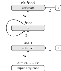
Figure 1: Neural network encoding the bag-of-words model. The output layer is discarded after training and the histograms from the recurrent layer are used for classification in combination with a support vector machine.

3.3 Equivalence Results

There is a close relation between single-layer neural networks and Gaussian models [35, 36]. We consider the special case of kMeans here. Following the derivation in the previous section, the kMeans model can be transformed into a single-layer neural network. For the other direction, however, the constraint that the bias components are inner products of the weight matrix rows (see Equations (12) and (13)) is not met when optimizing the neural network parameters. In fact, the single-layer neural network is equivalent to a kMeans model with non-uniform visual word priors $p(v_{m})$. While the transformation from a kMeans model to a neural network is defined by Equations (12) and (13), the transformation from the neural network model to a kMeans model is given by

$$v_{m} =(\mathbf{W}_{1,m}\dots\mathbf{W}_{D,m})^{\intercal},$$ (20)

$$p_{\mathrm{NN}}(v_{m}) =\frac{\exp{(b_{m}+\frac{1}{2}v_{m}^{\intercal}v_{m})}}{\sum_{\tilde{m}}\exp{(b_{\tilde{m}}+\frac{1}{2}v_{\tilde{m}}^{\intercal}v_{\tilde{m}})}}.$$ (21)

3.4 Encoding Kernels in the Neural Network

So far, the recurrent neural network is capable of computing bag-of-words like histograms that are then used in a support vector machine in combination with a kernel. In this section, we show how to incorporate the kernel itself into the neural network.

Consider the histograms $h_{1}$ and $h_{2}$ of two input sequences $\mathbf{x}$ and $\mathbf{y}$,

$$h_{1}=\mathcal{H}(\mathbf{x}),\quad h_{2}=\mathcal{H}(\mathbf{y})\in\mathbb{R}^{M}.$$ (22)

A kernel $\mathcal{K}(h_{1},h_{2})$ is defined as the inner product

$$\mathcal{K}(h_{1},h_{2})=\langle\Psi(h_{1}),\Psi(h_{2})\rangle,$$ (23)

where $\Psi$ is the feature map inducing the kernel. In general, it is difficult to find an explicit formulation of $\Psi$. In [37], Vedaldi and Zisserman provide an explicit (approximate) representation for additive homogeneous kernels. A kernel is called additive if

$$\mathcal{K}(h_{1},h_{2})=\sum_{m=1}^{M}k(h_{1,m},h_{2,m}),$$ (24)

where $k:\mathbb{R}_{0}^{+}\times\mathbb{R}_{0}^{+}\mapsto\mathbb{R}_{0}^{+}$ is a kernel induced by a feature map $\psi$. $k$ is homogeneous if

$$k(\alpha h_{1,m},\alpha h_{2,m})=\alpha k(h_{1,m},h_{2,m}).$$ (25)

According to [37], the feature map $\psi$ for such kernels is approximated by

$$[\psi(x)]_{j}=\begin{cases}\sqrt{\kappa(0)xL}&j=0,\\ \sqrt{2\kappa(\frac{j+1}{2}L)xL}\cos(\frac{j+1}{2}L\log x)&j\text{ odd},\\ \sqrt{2\kappa(\frac{j}{2}L)xL}\sin(\frac{j}{2}L\log x)&j\text{ even},\end{cases}$$ (26)

where $\kappa$ is a function dependent on the kernel, $L$ is a sampling period, and $0\leq j\leq 2n$ defines the number of samples, see [37] for details.

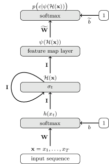
Figure 2: Neural network encoding the bag-of-words model and a kernel via its feature map.

The function $[\psi(x)]_{j}$ is continuously differentiable on the non-negative real numbers and the derivative is given by

$$\frac{\partial[\psi(x)]_{j}}{\partial x}=\begin{cases}[\psi(x)]_{0}\gamma(x)&j=0,\\ ([\psi(x)]_{j+1}(j+1)L+[\psi(x)]_{j})\gamma(x)&j\text{ odd},\\ ([\psi(x)]_{j-1}jL+[\psi(x)]_{j})\gamma(x)&j\text{ even},\end{cases}$$ (27)

where

$$\gamma(x)=\frac{\kappa(0)L}{2[\psi(x)]_{0}^{2}}.$$ (28)

Since we apply kernels to histograms, the input to a feature map is always non-negative in our case. Hence, Equation (26) can be implemented as a layer in a neural network. Adding such a feature map layer between the recurrent layer and the softmax output allows to represent the bag-of-words pipeline including support vector machine and kernel computations completely in a single neural network, cf. Figure 2.

To illustrate that this modification of the neural network is in fact sufficient to model a support vector machine with a non-linear kernel, consider a simple two class problem. The classification rule for the support vector machine is then

$$r_{\text{SVM}}(\mathcal{H}(\mathbf{x}))=\mathrm{sgn}\Big{(}\sum_{i=1}^{I}\alpha_{i}y_{i}\mathcal{K}(\mathcal{H}(\mathbf{x}_{i}),\mathcal{H}(\mathbf{x}))+b\Big{)}$$ (29)

with $I$ support vectors and coefficients $\alpha_{i}$ as well as labels $y_{i}\in\{-1,1\}$. Defining

$$\mathbf{w}_{c}=\sum_{i=1}^{I}\alpha_{i}y_{i}\Psi(\mathcal{H}(\mathbf{x}_{i}))$$ (30)

allows to simplify the decision rule to

$$r_{\text{SVM}}(\mathcal{H}(\mathbf{x}))=\mathrm{sgn}\big{(}\langle\mathbf{w}_{c},\Psi(\mathcal{H}(\mathbf{x}))\rangle+b\big{)}.$$ (31)

As can be seen from this equation, the decision rule is an inner product of a weight vector and the feature map $\psi(\mathcal{H}(\mathbf{x}))$. This is the same operation that is performed in the neural network, apart from the $\mathrm{softmax}$ output layer. This, however, does not affect the maximizing argument, so the decision of the support vector machine and the decision of the neural network are the same if the same weights and bias are used. Still, in contrast to the support vector machine, the neural network is trained according to the cross-entropy criterion using unconstrained optimization. So in practice, the neural network model usually differs from the model obtained with a support vector machine.

Note that the approximate feature map increases the dimension and, thus, also the number of parameters, depending on the number of samples. If the histograms are of dimension $M$, the output of the feature map layer is of dimension $M\cdot(2n+1)$. In practice, however, $n=2$ already works well [37].

3.5 Implementation Details

Neural networks are usually optimized using gradient based methods such as stochastic gradient descent (SGD) or Resilient Propagation (RProp; [38]). The gradient of a recurrent neural network can be efficiently computed using backpropagation through time (BPTT; [39]). In a forward pass, the activation $y_{l,t}$ of each layer $l$ is computed for all timeframes $t$. The corresponding error signals $e_{l,t}$ are then computed in a backward pass through all layers and timeframes. Thereby, it is necessary to keep all $y_{l,t}$ in memory during backpropagation. For long input sequences, this may be prohibitive since neural networks are usually optimized on a GPU that has only a few GB of memory.

Our model is a specific kind of neural network with only a single recurrent connection that has the unit matrix as weights. Two special properties emerge from this structure. First, the order in which the input sequence $x_{1},\dots,x_{T}$ is presented to the network does not affect the output. Second, the error signals of the recurrent layer are the same for each timeframe, i.e.

$$e_{\mathrm{rec},T}=e_{\mathrm{rec},t}\quad\text{ for }t=1,\dots,T.$$ (32)

Thus, it is sufficient to store $e_{\mathrm{rec},T}$ once and then process each feature vector in another pass through the network using standard error backpropagation [40], which requires much less memory. The training process is illustrated in Algorithm 1. We indicate the first $\mathrm{softmax}$ layer, the recurrent layer, the feature map, and the output layer as sft, rec, map, and out, respectively. Further, $\mathbb{I}_{c}$ is used to indicate the unit vector with a one in its $c$-th component and $\mathbf{J}_{f}(a)$ is the Jacobi matrix of a function $f$ at $a$. Given an input sequence $\mathbf{x}$, the activations of the output layer are computed in a forward pass. In the following backward pass, the error signals for each timeframe are used to accumulate the gradients. Note that the algorithm is a special case of BPTT. Due to the trivial recurrent connection, the activations and error signals at times $t<T$ do not need to be stored once the error signal $e_{\mathrm{rec},T}$ is computed.

Algorithm 1 Memory efficient gradient computation

1:input: feature sequence $\mathbf{x}$

2:initialize $\Delta\mathbf{W},\Delta\mathbf{\widetilde{W}},\Delta b,\Delta\tilde{b}$ with zero

3:procedure forward-pass

4:     for $t=1,\dots,T$ do

5:         $y_{\mathrm{sft},t}\leftarrow\mathrm{softmax}(\mathbf{W}^{\intercal}x_{t}+b)$

6:         $y_{\mathrm{rec},t}\leftarrow\sigma_{t}(y_{\mathrm{sft},t}+y_{\mathrm{rec},t-1})$

7:         delete $y_{\mathrm{sft},t}$ and $y_{\mathrm{rec},t-1}$      

8:     $y_{\mathrm{map},T}\leftarrow\psi(y_{\mathrm{rec},T})$

9:     $y_{\mathrm{out},T}\leftarrow\mathrm{softmax}(\mathbf{\widetilde{W}}^{\intercal}y_{\mathrm{map},T}+\tilde{b})$

10:procedure backward-pass

11:     $e_{\mathrm{out},T}\leftarrow y_{\mathrm{out},T}-\mathbb{I}_{c}$

12:     $e_{\mathrm{map},T}\leftarrow\mathbf{J}_{\psi}(y_{\mathrm{rec},T})\cdot\mathbf{\widetilde{W}}\cdot e_{\mathrm{out},T}$

13:     $e_{\mathrm{rec},T}\leftarrow\mathbf{J}_{\sigma_{T}}(y_{\mathrm{sft},T})\cdot e_{\mathrm{map},T}$

14:     for $t=1,\dots,T$ do

15:         $e_{\mathrm{sft},t}\leftarrow\mathbf{J}_{\mathrm{softmax}}(\mathbf{W}^{\intercal}x_{t}+b)\cdot e_{\mathrm{rec},T}$

16:         $\Delta\mathbf{W}\leftarrow\Delta\mathbf{W}+x_{t}\cdot e_{\mathrm{sft},t}^{\intercal}$

17:         $\Delta b\leftarrow\Delta b+e_{\mathrm{sft},t}$      

18:     $\Delta\mathbf{\widetilde{W}}\leftarrow y_{\mathrm{map},T}\cdot e_{\mathrm{out},T}^{\intercal}$

19:     $\Delta\tilde{b}\leftarrow e_{\mathrm{out},T}^{\intercal}$ return $\Delta\mathbf{W},\Delta\mathbf{\widetilde{W}},\Delta b,\Delta\tilde{b}$

4 Experimental Setup

4.1 Feature Extraction

We extract improved dense trajectories as described in [8], resulting in five descriptors with an overall number of 426 features per trajectory, and apply z-score normalization to the data. We distinguish between two kinds of features: concatenated and separated descriptors. For the first, all $426$ components of a trajectory are treated as one feature vector. For the latter, the dense trajectories are split into their five feature types Traj, HOG, HOF, and two motion boundary histograms MBHX and MHBY in $x$- and $y$-direction.

4.2 kMeans Baseline

For the baseline, we follow the approach of [7]: kMeans is run eight times on a randomly sampled subset of $100,000$ trajectories. The result with lowest sum of squared distances is used as visual vocabulary. For concatenated descriptors, a histogram of $4,000$ visual words is created based on the $426$-dimensional dense trajectories. In case of separate descriptors, a visual vocabulary with $4,000$ visual words is computed for each descriptor type separately. The resulting five histograms are combined with a multichannel RBF-$\chi^{2}$ kernel as proposed in [7],

$$\mathcal{K}(i,j)=\exp{\bigg{(}-\frac{1}{5}\sum_{c=1}^{5}\frac{D(\mathcal{H}(\mathbf{x}_{i}^{c}),\mathcal{H}(\mathbf{x}_{j}^{c}))}{A_{c}}\bigg{)}},$$ (33)

where $\mathbf{x}_{i}^{c}$ is the $c$-th descriptor type of the $i$-th video, $D(\cdot,\cdot)$ is the $\chi^{2}$-distance between two histograms, and $A_{c}$ is the mean distance between all histograms for descriptor $c$ in the training set. For concatenated features, the kernel is used with a single channel only. As classifier, we train a one-against-rest support vector machine using LIBSVM [41].

4.3 Neural Network Setup

When training neural networks, the trajectories of each video are uniformly subsampled to reduce the total amount of trajectories. The network is trained according to the cross-entropy criterion, which maximizes the likelihood of the posterior probabilities. We use RProp as optimization algorithm and iterate until the objective function does not improve further. If the neural network output is not directly used for classification, i.e. if a support vector machine is used to classify the histograms generated by the neural network, overfitting is not a critical issue. Thus, strategies like regularization or dropout do not need to be applied. Furthermore, we could not investigate any advantages when initializing with a kMeans model. Normalization, in contrast, is crucial. If the network input is not normalized, the training of the neural network is highly sensitive to the learning rate and RProp even fails to converge. For consistency with the kMeans baseline, the number of units in the first $\mathrm{softmax}$ layer and the recurrent layer that computes the histograms is also set to $4,000$.

4.4 Datasets

For the evaluation of our method, we use four action recognition benchmarks, two of which are of medium and two of large scale.

With $783$ action clips from $16$ classes, the Olympic Sports dataset [42] is the smallest among the four benchmarks. The videos show athletes performing Olympic disciplines and are several seconds long. We use the train/test split suggested in [42], which partitions the dataset into $649$ training videos and $134$ test instances. After extracting improved dense trajectories, the training set comprises about $40$ million trajectories and the test set $7.8$ million. For evaluation, mean average precision is reported.

HMDB-51 [43] is a large scale action recognition benchmark containing $6,849$ clips of $51$ different classes. The clips are collected from public databases and movies. In contrast to Olympic Sports, the clips in HMDB-51 are usually only a few seconds long. The dataset provides at least $101$ instances of each action class and the authors propose a three-fold cross validation. All splits are of comparable size and after feature extraction, there are $42$ million trajectories in the training set and $18$ million in the test set. We report average accuracy over the splits.

In order to validate the applicability of our method to datasets of different sizes, we also conduct experiments on a subset of HMDB-51. J-HMDB [11] comprises a subset of $928$ videos from $21$ action classes. With a range from $15$ to $40$ frames, the clips are rather short. We follow the protocol of [11] and use three splits. Each split partitions the videos into training and test set with an approximate ratio of $70:30$. For the training set, about two million trajectories are extracted for each split. For the test set, the amount of extracted trajectories ranges between $700,000$ and $800,000$ depending on the split. Even though the number of clips in the dataset is in the same order as for Olympic Sports, it is clearly the smallest dataset in our evaluation in terms of extracted trajectories. As for HMDB-51, average accuracy over the three splits is reported.

The largest benchmark we use is the UCF101 dataset [44]. Comprising $13,320$ video clips from a set of $101$ different action classes, it is about twice as large as HMDB-51. The dataset contains videos from five major categories (sports, human-human-interaction, playing musical instruments, body-motion only, and human-object interaction) and has been collected from Youtube. Again, we follow the protocol of [44] and use the suggested three splits. Each split partitions the data in roughly $9,500$ training clips and $3,700$ test clips, corresponding to $230$ million improved trajectories for the training set and $90$ million for the test set, respectively. Again, we report average accuracy over the three splits.

For Olympic Sports and HMDB-51, we use the human bounding boxes provided by Wang and Schmid. For the other datasets, improved dense trajectories are extracted without human bounding boxes.

5 Experimental Results

In this section, we evaluate our method empirically. In a first step, the impact of the prior and the difference in the histograms generated by a standard kMeans model and our neural network are analyzed. Then, the effect of subsampling the dense trajectories is investigated. We show that even with a small number of trajectories, satisfying results can be obtained while accelerating the training time by up to two orders of magnitude. Moreover, we compare our model to the standard pipeline for action recognition from [7, 8] and show that the method is not only bound to action recognition but is also competitive to some well known sparse coding methods in image classification. We also evaluate the effect approximating the kernel directly within the neural network as proposed in Section 3.4, followed by a comparison to the current state-of-the-art in action recognition.

5.1 Evaluation of the Neural Network Model

(a) kMeans prior $p_{\mathrm{KM}}(v_{m})$

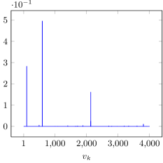
(b) neural network prior $p_{\mathrm{NN}}(v_{m})$

Figure 3: Comparison of the visual word prior induced by kMeans and the prior obtained with the neural network on the Olympic Sports dataset. Note the different scales on the $y$-axes.

           

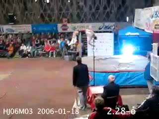
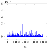
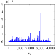
(a) Example frame (left), kMeans histogram (middle), and neural network histogram (right) for the video high_jump/010.avi.

           

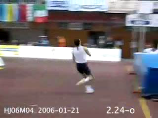
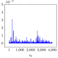
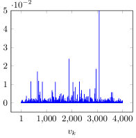
(b) Example frame (left), kMeans histogram (middle), and neural network histogram (right) for the video high_jump/011.avi.

           

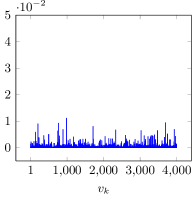
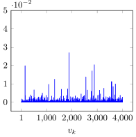
(c) Example frame (left), kMeans histogram (middle), and neural network histogram (right) for the video pole_vault/001.avi.

           

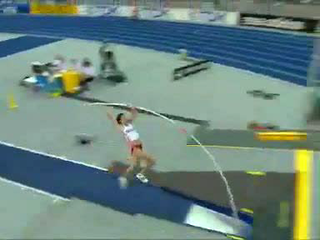
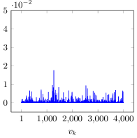
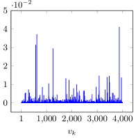
(d) Example frame (left), kMeans histogram (middle), and neural network histogram (right) for the video pole_vault/005.avi.

Figure 4: Comparison of the histograms generated by the kMeans model and the neural network model for four videos of two different classes from Olympic Sports.

We evaluate the neural network model by comparing its performance on Olympic Sports to the performance of the kMeans based bag-of-words model. Moreover, we analyze the difference between the histograms generated by the neural network and those generated by the kMeans approach. For neural network training, the number of trajectories per video is limited to $5,000$ using uniform subsampling.

As mentioned in Section 3, the neural network implicitly models a visual word prior $p_{\mathrm{NN}}(v_{m})$. Hence, we compare to an additional version of kMeans in which we compute the posterior distribution $p_{\mathrm{KM}}(v_{m}|x)$ with a non-uniform prior $p_{\mathrm{KM}}(v_{m})$. The prior is modeled as relative frequencies of the visual words. Note that the resulting model is equivalent to the neural network model and only differs in the way the parameters are estimated.

		assignment
		soft		hard
kMeans		$84.1\%$		$84.0\%$
kMeans + prior		$83.7\%$		$84.0\%$
neural network		$86.7\%$		$86.3\%$

Table 1: Comparison of three bag-of-words models: kMeans, kMeans with prior, and the neural network (Figure 1). For each model, the histograms are once computed using soft assignment, i.e. the posterior distribution $p(v_{m}|x)$ is used directly, and once using hard assignment, i.e. shifting all probability mass to the most likely visual word.

When computing histograms of visual words, usually hard assignment is used as in $\hat{p}_{\mathrm{KM}}(v_{m}|x)$ in Equation (9). This may be natural for kMeans since during the generation of the visual vocabulary, each observation only contributes to its nearest visual word. For the neural network model, on the contrary, hard assignment can not be used during training since differentiability is required. Thus, it is natural to use the posterior distribution $p_{\mathrm{NN}}(v_{m}|x)$ directly for the histogram computation. However, in Table 1 it can be seen that there is no significant difference between soft and hard assignment for either of the three methods.

Furthermore, Table 1 reveals that the neural network is more than $2\%$ better than the kMeans model. However, the improvement can not be explained by the additional degrees of freedom, as the kMeans model with non-uniform prior does not improve compared to the original kMeans model. Discriminative training allows the neural network to generate visual words that discriminate well between the classes. KMeans, in contrast, only generates visual words that represent the observation space well regardless of the class labels. We validate this major difference between both methods by a comparison of the visual word priors. In Figure 3a, the prior induced by kMeans, $p_{\mathrm{KM}}(v_{m})$, is illustrated. The probability for all visual words is within the same order of magnitude. The neural network prior $p_{\mathrm{NN}}(v_{m})$ is computed by means of Equation (21) and depicted in Figure 3b. Almost all probability mass is distributed over three visual words. All other visual words are extremely rare, making their occurrence in a histogram a very discriminative feature.

In Figure 4, the histograms generated by kMeans and the neural network are compared for four videos from two different classes, high_jump and pole_vault. The first column shows an example frame of the video. The second and third column show the histograms generated by the kMeans model and by the neural network, respectively. The histograms generated by the neural network are sharper than those generated by the kMeans model. The two peaks in the neural network histograms of the high_jump videos at visual word index $3,000$ are a pattern that occurs in multiple histograms of this class. Similar patterns can also be observed for neural network histograms of other classes but usually not for kMeans based histograms, although the example videos from high_jump are very similar in appearance. If the appearance of the videos undergoes stronger variations as in the pole_vault class, these reoccurring patterns are neither observable for the kMeans based histograms nor for the neural network histograms. Still, the latter have clearer peaks that lead to larger differences between histograms of different videos, raising potential for a better discrimination. This confirms the preceding evaluation of the results in Table 1.

During training of the neural network, a class posterior distribution $p(c|\mathcal{H}(\mathbf{x}))$ is modeled. Using this model instead of the SVM with RBF-$\chi^{2}$ kernel for classification is worse than the baseline. For concatenated descriptors, the result on Olympic Sports is $82.3\%$. Regularization, dropout, and adding additional layers did not yield any improvement. However, considering that the model for $p(c|\mathcal{H}(\mathbf{x}))$ is only a linear classifier on the histograms (cf. Section 3), the result is remarkable as the kMeans baseline with a linear support vector machine reaches only $69.6\%$.

5.2 Effect of Feature Subsampling

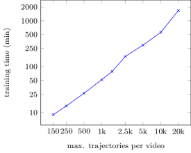
(a)

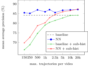
(b)

Figure 5: Effect of feature subsampling on the training time and the performance evaluated on Olympic Sports. Left: Time required to train the neural network. Right: Performance of the neural network (NN) based bag-of-words. For the blue curve, the number of trajectories has only been limited for neural network training. For the red and green curve, it has also been limited for the histogram computation on the training and test set (sub-hist).

We evaluate the runtime and accuracy of our method when reducing the number of trajectories per video on Olympic Sports. The networks are trained on a GeForce GTX $780$ with $3$GB memory. We limit the number of trajectories per video to values from $150$ to $20,000$ via uniform subsampling. This corresponds to an overall number of trajectories between $100,000$ and $12$ million. In Figure 5 (left), the runtime is shown. When sampling $150$ trajectories per video, which corresponds to $100,000$ dense trajectories overall, both, our GPU implementation of kMeans and the neural network training, run for nine minutes. The training times scales linearly with the number of trajectories per video. In Figure 5 (right), the performance of the system with limited number of trajectories is illustrated. For the blue curve, the number of trajectories has only been limited for neural network training, but the histograms are computed on all extracted trajectories. The performance of the neural network models is always above the baseline (dashed line). The curve stabilizes around $5,000$ trajectories per video, suggesting that this number is sufficient for the neural network based bag-of-words. Note that for kMeans, we observed only small fluctuations around one percent when changing the number of clustered trajectories, the subsampling strategy, or the initialization.

If the histograms for the training and test set are also computed on the limited set of trajectories (red and green curve), the performance of the systems is much more sensitive to the number of subsampled trajectories. However, when more than $5,000$ trajectories per video (overall $3.2$ million trajectories) are used for the neural network histogram computation, the difference to taking all extracted trajectories is small. Hence, it is possible to achieve satisfying results with only $8\%$ of the originally extracted trajectories, allowing to accelerate both, the histogram computation and the feature extraction itself. A similar reduction is also possible with kMeans, but the loss in accuracy is higher, cf. Figure 5.

5.3 Comparison to Other Neural Network Architectures

Method		mAP
Training on frame-level
(a)	ours w/o recurrency	$62.3\%$
(b)	fine-tuned ImageNet CNN	$76.6\%$
Training on video-level
(c)	simple RNN	$18.3\%$
(d)	RNN with GRUs	$13.3\%$
(e)	attention-based RNN	$28.8\%$
(f)	ours	$86.7\%$

Table 2: Comparison of different neural network architectures on Olympic Sports. Results are reported as mean average precision.

In this section, we compare our proposed model to other neural network architectures. Our analysis is twofold: firstly, we show the importance of video-level training, secondly, we prove that the bag-of-words equivalent architecture is crucial and other recurrent neural networks fail to obtain good results.

Addressing the first point, we remove the recurrent connection from our model. The result is a standard feed-forward network. For training, we assign to each input frame the class label of the respective video. For inference, we cut off the last softmax layer and compute a video representation by average pooling over the network output of each frame. Following the same protocol as for our recurrent network, the resulting representation is transformed with a multi-channel $\chi^{2}$ kernel and classified using a support vector machine. In this setup, each input frame is treated separately and temporal context is not considered during codebook training. The resulting loss of accuracy is significant: the performance drops from $86.7\%$ to $62.3\%$, cf. Table 2 (a) and (f). As another example for frame-level training, we fine-tuned the $51$-layer deep residual CNN of the $2015$ ImageNet challenge winning submission [45] on Olympic Sports. In order to get class posterior probabilities for a complete video, we applied average pooling to the framewise posteriors. Still, this state-of-the-art CNN architecture struggles to achieve competitive results.

Addressing the second point, we replace the bag-of-words equivalent architecture by other recurrent network architectures. Simple RNN (c) is a neural network with a single recurrent hidden layer and sigmoid activations. RNN with GRUs (d) has the same structure but the sigmoid units are replaced by gated recurrent units [46]. Those units allow the network to decide when to discard past frames and when to update the recurrent activations based on forget and update gates. Not surprisingly, the performance of both recurrent architectures is poor. Recurrent neural networks tend to forget about past inputs exponentially fast, so particularly for long sequences as we have in our setup, only the end of the video is actually observed and the crucial parts at the beginning and in the middle of the video are not considered. Attention-based RNNs [47] aim to solve this problem. An attention layer learns weights for each timeframe of a recurrent layer and accumulates the recurrent layer activations according to this weighting. This way, information is captured along the complete sequence. Unfortunately, these models have a large number of parameters and are highly sensitive to overfitting, especially in case of the huge intra-class variations in video data. Consequently, the classification result is better than for traditional recurrent neural networks but still not competitive to state-of-the-art methods, cf. Table 2 (e).

Summarizing, the results in Table 2 show that both the specific architecture and the joint training of classifier and vocabulary on video-level are crucial.

5.4 Evaluation on Various Datasets

Descriptors:		concatenated			separate
		baseline	neural network		baseline	neural network
Olympic Sports		$84.1\%$	$\mathbf{86.7\%}$		$84.4\%$	$\mathbf{85.9\%}$
J-HMDB		$56.6\%$	$\mathbf{57.6\%}$		$59.1\%$	$\mathbf{61.9\%}$
HMDB-51		$45.8\%$	$\mathbf{50.6\%}$		$52.2\%$	$\mathbf{54.0\%}$
UCF101		$67.8\%$	$\mathbf{73.3\%}$		$73.3\%$	$\mathbf{76.9\%}$

Table 3: Comparison of the kMeans baseline with the neural network model for concatenated and separate descriptors on four different datasets.

We evaluate our method on the four action recognition datasets Olympic Sports, J-HMDB, HMDB-51, and UCF101. On J-HMDB, all extracted trajectories are used for neural network training. On HMDB-51 and Olympic Sports, we limit the number of trajectories per video to $5,000$ as proposed in Section 5.2. For terms of efficiency, we further reduce this number to $2,500$ for the largest dataset UCF101. We conduct the experiments for concatenated descriptors, i.e. we directly use a $426$ dimensional feature vector for each trajectory, and for separate descriptors as originally proposed in [7]. The results are shown in Table 3.

The neural network outperforms the baseline on all datasets. For the smaller datasets J-HMDB and Olympic Sports that have only few classes, the improvement is between $1\%$ and $2.6\%$ in case of concatenated descriptors. For the large datasets, however, the baseline is outperformed by around $5\%$. In case of separate descriptors, the improvement is smaller but still ranges from $1.5\%$ to $3.6\%$.

Comparing the neural network with concatenated descriptors (second column of Table 3) and the baseline with separate descriptors (third column of Table 3) reveals that both systems achieve similar accuracies. However, for the baseline with separate descriptors, visual vocabularies and histograms have to be computed for each of the five descriptors separately. For the neural network with concatenated descriptors, in contrast, it is sufficient to train a single system.

5.5 Application to Image Classification

Method	Codebook Size	Caltech-101	15-Scenes
Hard assignment [48]	$200$	$64.6\%$	$81.1\%$
Kernel Codebooks [49]	$200$	$64.1\%$	$76.7\%$
Soft assignment [50]	$1000$	$74.2\%$	$82.7\%$
ScSPM [17]	$1024$	$73.2\%$	$80.3\%$
LLC [18]	$2048$	$73.4\%$	-
Multi-way local pooling [51]	$1024\times 65$	$77.8\%$	$83.1\%$
Unsupervised SS-RBM [19]	$1024$	$75.1\%$	$84.1\%$
Ours	$\mathbf{1024}$	$\mathbf{74.5\%}$	$\mathbf{83.5\%}$

Table 4: Comparison of our method to other coding methods on Caltech-101 and 15-scenes.

Although designed to meet some specific problems in action recognition, our method is applicable to image datasets, too. We compare to existing sparse coding methods on two small image datasets, Caltech-101 [52] and 15-scenes [53]. Following the setup of [19], we densely extract SIFT features, compute spatial pyramids, and use a linear support vector machine for classification. Note that our method is not particularly designed for such a setting since we do not train our encoding directly on the spatial pyramid features that are finally used for classification. In contrast to the methods [17, 18, 51, 19], we do not introduce any sparsity constraints. Still, our method shows competitive results compared to several other coding methods, see Table 4.

5.6 Using Explicit Feature Maps

In this section, we analyze the effect of explicit feature maps that allow to train the complete system in a single network. We use the network architecture from Figure 2. Since the multichannel RBF-$\chi^{2}$ kernel from Equation (33) is not an additive homogeneous kernel, we evaluate three different additive homogeneous kernels here: Hellinger’s kernel is defined as

$$k(h_{1,i},h_{2,i})=\sqrt{h_{1,i}h_{2,i}}$$ (34)

and its underlying feature map has an exact closed form solution, $\psi(x)=\sqrt{x}$. It is notable that due to the non-negativity of the histograms that are fed into the function, Hellinger’s kernel is equivalent to the application of power normalization that has been proposed for Fisher vectors in [6].

Moreover, we examine an additive homogeneous version of the $\chi^{2}$ kernel,

$$k(h_{1,i},h_{2,i})=2\frac{h_{1,i}h_{2,i}}{h_{1,i}+h_{2,i}}.$$ (35)

In combination with a support vector machine, the kernel can be applied directly. When incorporating it into the neural network, we use the approximation from Equation (26) with $\kappa(\lambda)=\mathrm{sech}(\pi\lambda)$. Finally, the histogram intersection kernel

$$k(h_{1,i},h_{2,i})=\min(h_{1,i},h_{2,i})$$ (36)

is approximated similarly with

$$\kappa(\lambda)=\frac{2}{\pi(1+4\lambda^{2})}.$$ (37)

Detailed derivations for the $\kappa$ functions can be found in [37]. As proposed in [37], we use $n=2$ and $L=0.5$ for both the $\chi^{2}$ kernel and the histogram intersection kernel. In case of concatenated descriptors, this increases the amount of units from $4,000$ in the histogram layer to $20,000$ in the feature map layer.

In order to be able to train a single neural network not only for concatenated descriptors but also for separate descriptors, each of the five descriptors is handled in an independent channel within the neural network allowing to train five independent visual vocabularies. After application of the feature map, the five channels are concatenated to a single channel five times the size of each feature map. A $\mathrm{softmax}$ layer is used for classification on top of the concatenated channel. As a consequence, the number of units after application of the feature map is five times larger than for concatenated descriptors, finally ending up with $100,000$ units. This affects the runtime for both, training and recognition, and can be particularly important for larger datasets.

The application of Hellinger’s kernel, the $\chi^{2}$ kernel, and the histogram intersection kernel in combination with a support vector machine for concatenated descriptors is straightforward. In case of separate descriptors, we combine the five histograms by concatenation.

		concatenated				separate
feature map:		Hellinger	$\chi^{2}$	hist. int.		Hellinger	$\chi^{2}$	hist. int.
Olympic Sports
from scratch		$75.5$	$84.1$	$82.9$		$84.3$	$81.4$	$80.4$
init linear		$81.3$	$85.0$	$83.8$		$83.7$	$83.0$	$83.0$
retrain top		$86.4$	$85.8$	$85.8$		$78.5$	$83.5$	$84.1$
J-HMDB
from scratch		$53.2$	$52.8$	$52.4$		$56.9$	$45.9$	$46.2$
init linear		$50.6$	$55.1$	$53.6$		$57.9$	$57.2$	$61.4$
retrain top		$57.5$	$56.6$	$56.7$		$56.9$	$60.9$	$60.5$

Table 5: Different training strategies when using a feature map layer.

We start with an evaluation of three different neural network training approaches on the two smaller datasets J-HMDB and Olympic Sports. Training from scratch starts with a random initialization of all parameters, init linear initializes the weights $\mathbf{W}$ and bias $\mathbf{b}$ with those obtained from the network from Figure 1 which is trained with a linear $\mathrm{softmax}$ classifier on top of the histogram layer. For retrain top we took the same initialization but kept it fixed during training and only optimized the parameters of the softmax output layer.

The results are shown in Table 5. For concatenated descriptors, retraining only the top layer leads to the best results for each feature map on both datasets and training from scratch performs worst in most cases. For separate descriptors, however, retrain top is not always best. Particularly on Olympic Sports, Hellinger’s kernel fails to achieve competitive results. Still, for all other cases retrain top is either best or at least close to the best training strategy. Since it is the fastest among the three strategies, we find it beneficial particularly for larger datasets.

Based on these results, we stick to the retrain top strategy for large datasets and compare the results to the traditional bag-of-words model and the neural network plus support vector machine model from Section 3.2. Table 6 shows the results of each of the three approaches for three different kernels and both concatenated and separate descriptors. The fourth and eighth column contain the numbers from Table 3 in order to provide a comparison to the originally used multichannel RBF-$\chi^{2}$ kernel. Recall that this kernel is not homogeneous and additive, so it can not be modeled as a neural network layer.

For concatenated descriptors, both neural network approaches usually outperform the kMeans baseline. While the difference between the kMeans baseline (kMeans + SVM) and the neural network including the feature map layer (retrain top) is rather small, a huge improvement can be observed for the neural network based visual words in combination with a support vector machine (neural network + SVM). Especially on the larger datasets HMDB-51 and UCF101, about $6\%$ improvement is achieved. This is particularly remarkable as the performance of a traditional bag-of-words model with separate descriptors is almost reached although the model with concatenated descriptors is much simpler: Only a single visual vocabulary with $4,000$ visual words is computed, while separate descriptors have an own visual vocabulary for each descriptor type, resulting in a five times larger representation.

Analyzing the results for separate descriptors, the neural network with a feature map corresponding to Hellinger’s kernel shows surprisingly bad results on all datasets. One explanation is that the feature map is simply the square root of each histogram entry, while for all other kernels the approximate feature map from Equation (26) has to be used. The number of units in the feature map layer is increased in the latter case, raising potential for a better discrimination.

Similar to the results of concatenated descriptors, the neural network combined with a support vector machine achieves the best results, whereas the neural network with a feature map layer yields results comparable to the traditional bag-of-words model. On all datasets, the best results have been obtained with separate descriptors and a neural network plus support vector machine using a $\chi^{2}$ kernel, see second row, sixth column for each dataset. Still, including a feature map layer also shows competitive results in most cases while considerably reducing the runtime. Especially on UCF101, the largest of the datasets, computation of a non-linear kernel and training a support vector machine takes $3.9$ hours, which is about six times longer than the time needed to retrain the neural network with the feature map layer ($40$ minutes).

A comparison of the results in Table 6 reveals that the multichannel RBF-$\chi^{2}$ kernel as used in [7] does not achieve as good results as a simple $\chi^{2}$ kernel with feature concatenation.

		concatenated					separate
				hist.	RBF-$\chi^{2}$				hist.	RBF-$\chi^{2}$
feature map:		Hellinger	$\chi^{2}$	int.	Eq. (33)		Hellinger	$\chi^{2}$	int.	Eq. (33)
Olympic Sports
kMeans + SVM		$83.7$	$84.2$	$85.5$	$84.1$		$85.9$	$87.1$	$86.6$	$84.4$
neural network + SVM		$85.0$	$83.0$	$86.6$	$86.7$		$86.4$	$\mathbf{88.1}$	$87.5$	$85.9$
neural network (retrain top)		$86.6$	$85.8$	$85.8$	-		$78.5$	$83.5$	$84.1$	-
J-HMDB
kMeans + SVM		$57.1$	$56.0$	$56.8$	$56.6$		$60.9$	$60.0$	$59.8$	$59.1$
neural network + SVM		$59.4$	$58.5$	$58.3$	$57.6$		$\mathbf{62.8}$	$62.2$	$61.9$	$61.9$
neural network (retrain top)		$57.5$	$56.6$	$56.7$	-		$56.9$	$60.9$	$60.5$	-
HMDB-51
kMeans + SVM		$42.1$	$43.9$	$44.0$	$45.8$		$51.4$	$52.4$	$51.5$	$52.2$
neural network + SVM		$48.0$	$49.3$	$50.0$	$50.6$		$53.6$	$\mathbf{54.9}$	$54.3$	$54.0$
neural network (retrain top)		$44.0$	$47.3$	$47.4$	-		$47.9$	$50.2$	$50.0$	-
UCF101
kMeans + SVM		$72.2$	$73.1$	$72.2$	$67.8$		$79.2$	$79.5$	$78.7$	$73.3$
neural network + SVM		$78.8$	$78.6$	$77.7$	$73.3$		$81.7$	$\mathbf{81.9}$	$81.1$	$76.9$
neural network (retrain top)		$72.7$	$73.5$	$73.3$	-		$73.5$	$75.7$	$75.7$	-

Table 6: Evaluation of different kernels for the kMeans baseline, the neural network approach with support vector machine classification, and the neural network including a feature map layer. For the latter, we use the retrain top strategy.

5.7 Comparison to State of the Art

Method	HMDB-51		UCF101
Traditional models
Improved DT + bag of words	$52.2\%$		$73.3\%$
Improved DT + Fisher vectors [8, 54] (*)	$57.2\%$		$85.9\%$
Improved DT + LLC	$50.8\%$		$71.9\%$
Stacked Fisher vectors [22] (*)	$66.8\%$		-
Multi-skip feature stacking [55] (*)	$65.4\%$		$89.1\%$
Super-sparse coding vector [56]	$53.9\%$		-
Motion-part regularization [26] (*)	$65.5\%$		-
MoFap [25] (*)	$61.7\%$		$88.3\%$
Neural networks
Two-stream CNN [30] (**)	$59.4\%$		$88.0\%$
Slow-fusion spatio-temporal CNN [29] (**)	-		$65.4\%$
Composite LSTM [32]	$44.0\%$		$75.8\%$
TDD + improved DT with Fisher vectors [57] (*)	$65.9\%$		$91.5\%$
factorized spatio-temporal CNN [58]	$59.1\%$		$88.1\%$
Ours	$\mathbf{54.9\%}$		$\mathbf{81.9\%}$

Table 7: Comparison of our model to published results on HMDB-51 and UCF101. We also provide results with bag-of-words and LLC encoding as a direct comparison to our method. Methods marked with (*) use Fisher vectors, those marked with (**) use additional training data.

In Table 7, our best results - a neural network without feature map layer and a non-multichannel $\chi^{2}$ kernel - are compared to the state-of-the-art on HMDB-51 and UCF101. Our approach outperforms other approaches based on bag-of-words, sparse coding [56], locality constrained linear coding (LLC) [18], or neural networks [29, 32]. Particularly on UCF101, the improvement of $8\%$ compared to the original bag-of-words based pipeline is remarkable. The approach [30] is not directly comparable since the accuracy is mainly boosted by the use of additional training data. The approach of [58] outperforms our method. This method uses a large convolutional neural network consisting of multiple spatial convolution layers and a temporal convolution to enable modeling actions of different speeds. Apart from that method, only the methods that use Fisher vectors achieve a better accuracy than our method. However, extracting Fisher vectors is more expensive in terms of memory than a bag-of-words model. If Fisher vectors are extracted per frame, the storage of the features would require around 1 TB for the $2.4$ million frames of UCF101 compared to 35 GB for our method. For applications with memory and runtime constraints, our approach is a very useful alternative.

6 Conclusion

In this work, we have proposed a recurrent neural network that allows for discriminative and supervised visual vocabulary generation. In contrast to many existing coding and CNN based methods, our method can be applied on video level directly. Apart from kernel approximations via explicit feature maps, the network is equivalent to the traditional bag-of-words approach and differs only in the way it is trained. Although the best results could be obtained using the neural network for visual vocabulary generation and a support vector machine for classification, we have shown that it is possible to also include the kernel and classification steps into the network while retaining the performance of the original bag-of-words model. Our model has been particularly beneficial for large scale datasets. Moreover, it allows for a significant reduction in the amount of extracted features, speeding up training time and inference without a considerable loss in performance. Finally, our model can also be applied to other tasks like image classification. The neural network proves to be competitive with other methods that introduce additional constraints like sparsity.

Acknowledgments

Authors acknowledge financial support by the ERC starting grant ARCA (677650).

References

References

- [1] G. Csurka, C. Dance, L. Fan, J. Willamowski, C. Bray, Visual categorization with bags of keypoints, in: ECCV Workshop on statistical learning in computer vision, 2004.
- [2] J. Sivic, B. C. Russell, A. A. Efros, A. Zisserman, W. T. Freeman, Discovering object categories in image collections, Tech. rep., Massachusetts Institute of Technology (2005).
- [3] J. Zhang, M. Marszałek, S. Lazebnik, C. Schmid, Local features and kernels for classification of texture and object categories: A comprehensive study, International Journal on Computer Vision 73 (2007) 213–238.
- [4] J. Sivic, A. Zisserman, Video google: a text retrieval approach to object matching in videos, in: Int. Conf. on Computer Vision, 2003, pp. 1470–1477.
- [5] A. Krizhevsky, I. Sutskever, G. E. Hinton, Imagenet classification with deep convolutional neural networks, in: Advances in Neural Information Processing Systems, 2012, pp. 1097–1105.
- [6] F. Perronnin, J. Sánchez, T. Mensink, Improving the Fisher kernel for large-scale image classification, in: European Conf. on Computer Vision, 2010, pp. 143–156.
- [7] H. Wang, A. Kläser, C. Schmid, C.-L. Liu, Dense trajectories and motion boundary descriptors for action recognition, International Journal on Computer Vision 103 (2013) 60–79.
- [8] H. Wang, C. Schmid, Action recognition with improved trajectories, in: Int. Conf. on Computer Vision, 2013, pp. 3551–3558.
- [9] E. H. Taralova, F. De la Torre, M. Hebert, Motion words for videos, in: European Conf. on Computer Vision, 2014, pp. 725–740.
- [10] K. K. Reddy, M. Shah, Recognizing 50 human action categories of web videos, Machine Vision and Applications 24 (2013) 971–981.
- [11] H. Jhuang, J. Gall, S. Zuffi, C. Schmid, M. J. Black, Towards understanding action recognition, in: Int. Conf. on Computer Vision, 2013, pp. 3192–3199.
- [12] X. Peng, L. Wang, X. Wang, Y. Qiao, Bag of visual words and fusion methods for action recognition: Comprehensive study and good practice, Computer Vision and Image Understanding.
- [13] A. Richard, J. Gall, A bow-equivalent recurrent neural network for action recognition, in: British Machine Vision Conference, 2015.
- [14] F. Perronnin, C. Dance, G. Csurka, M. Bressan, Adapted vocabularies for generic visual categorization, in: European Conf. on Computer Vision, 2006, pp. 464–475.
- [15] H. Cai, F. Yan, K. Mikolajczyk, Learning weights for codebook in image classification and retrieval, in: IEEE Conf. on Computer Vision and Pattern Recognition, 2010, pp. 2320–2327.
- [16] X.-C. Lian, Z. Li, C. Wang, B.-L. Lu, L. Zhang, Probabilistic models for supervised dictionary learning, in: IEEE Conf. on Computer Vision and Pattern Recognition, 2010, pp. 2305–2312.
- [17] J. Yang, K. Yu, Y. Gong, T. Huang, Linear spatial pyramid matching using sparse coding for image classification, in: IEEE Conf. on Computer Vision and Pattern Recognition, 2009, pp. 1794–1801.
- [18] J. Wang, J. Yang, K. Yu, F. Lv, T. Huang, Y. Gong, Locality-constrained linear coding for image classification, in: IEEE Conf. on Computer Vision and Pattern Recognition, 2010, pp. 3360–3367.
- [19] H. Goh, N. Thome, M. Cord, J.-H. Lim, Unsupervised and supervised visual codes with restricted boltzmann machines, in: European Conf. on Computer Vision, 2012, pp. 298–311.
- [20] Y.-L. Boureau, F. Bach, Y. LeCun, J. Ponce, Learning mid-level features for recognition, in: IEEE Conf. on Computer Vision and Pattern Recognition, 2010, pp. 2559–2566.
- [21] H. Jégou, F. Perronnin, M. Douze, J. Sanchez, P. Perez, C. Schmid, Aggregating local image descriptors into compact codes, IEEE Transactions on Pattern Analysis and Machine Intelligence 34 (2012) 1704–1716.
- [22] X. Peng, C. Zou, Y. Qiao, Q. Peng, Action recognition with stacked Fisher vectors, in: European Conf. on Computer Vision, 2014, pp. 581–595.
- [23] D. Oneata, J. Verbeek, C. Schmid, Action and event recognition with Fisher vectors on a compact feature set, in: Int. Conf. on Computer Vision, 2013, pp. 1817–1824.
- [24] K. Simonyan, A. Vedaldi, A. Zisserman, Deep Fisher networks for large-scale image classification, in: Advances in Neural Information Processing Systems, 2013, pp. 163–171.
- [25] L. Wang, Y. Qiao, X. Tang, Mofap: A multi-level representation for action recognition, International Journal on Computer Vision 119 (3) (2016) 254–271.
- [26] B. Ni, P. Moulin, X. Yang, S. Yan, Motion part regularization: Improving action recognition via trajectory selection, in: IEEE Conf. on Computer Vision and Pattern Recognition, 2015, pp. 3698–3706.
- [27] X. Peng, L. Wang, Y. Qiao, Q. Peng, Boosting vlad with supervised dictionary learning and high-order statistics, in: European Conf. on Computer Vision, 2014, pp. 660–674.
- [28] V. Sydorov, M. Sakurada, C. H. Lampert, Deep Fisher kernels–end to end learning of the Fisher kernel Gmm parameters, in: IEEE Conf. on Computer Vision and Pattern Recognition, 2014, pp. 1402–1409.
- [29] A. Karpathy, G. Toderici, S. Shetty, T. Leung, R. Sukthankar, L. Fei-Fei, Large-scale video classification with convolutional neural networks, in: IEEE Conf. on Computer Vision and Pattern Recognition, 2014, pp. 1725–1732.
- [30] K. Simonyan, A. Zisserman, Two-stream convolutional networks for action recognition in videos, in: Advances in Neural Information Processing Systems, 2014, pp. 568–576.
- [31] J. Donahue, L. A. Hendricks, S. Guadarrama, M. Rohrbach, S. Venugopalan, K. Saenko, T. Darrell, Long-term recurrent convolutional networks for visual recognition and description, in: IEEE Conf. on Computer Vision and Pattern Recognition, 2015, pp. 2625–2634.
- [32] N. Srivastava, E. Mansimov, R. Salakhutdinov, Unsupervised learning of video representations using LSTMs, in: Int. Conf. on Machine Learning, 2015.
- [33] M. Jain, J. C. van Gemert, C. G. M. Snoek, What do 15,000 object categories tell us about classifying and localizing actions?, in: IEEE Conf. on Computer Vision and Pattern Recognition, 2015, pp. 46–55.
- [34] L. Wang, Y. Qiao, X. Tang, Action recognition with trajectory-pooled deep-convolutional descriptors, in: IEEE Conf. on Computer Vision and Pattern Recognition, 2015, pp. 4305–4314.
- [35] W. Macherey, H. Ney, A comparative study on maximum entropy and discriminative training for acoustic modeling in automatic speech recognition., in: Interspeech, 2003.
- [36] G. Heigold, R. Schlüter, H. Ney, On the equivalence of Gaussian HMM and Gaussian HMM-like hidden conditional random fields., in: Interspeech, 2007, pp. 1721–1724.
- [37] A. Vedaldi, A. Zisserman, Efficient additive kernels via explicit feature maps, IEEE Transactions on Pattern Analysis and Machine Intelligence (2012) 480–492.
- [38] M. Riedmiller, H. Braun, A direct adaptive method for faster backpropagation learning: The rprop algorithm, in: IEEE Int. Conf. on Neural Networks, 1993, pp. 586–591.
- [39] P. J. Werbos, Backpropagation through time: what it does and how to do it, Proceedings of the IEEE 78 (1990) 1550–1560.
- [40] D. E. Rumelhart, G. E. Hinton, R. J. Williams, Learning representations by back-propagating errors, Nature 323 (1986) 533–536.
- [41] C.-C. Chang, C.-J. Lin, Libsvm: a library for support vector machines, ACM Transactions on Intelligent Systems and Technology 2 (2011) 1–27.
- [42] J. C. Niebles, C.-W. Chen, L. Fei-Fei, Modeling temporal structure of decomposable motion segments for activity classification, in: European Conf. on Computer Vision, 2010, pp. 392–405.
- [43] H. Kuehne, H. Jhuang, E. Garrote, T. Poggio, T. Serre, HMDB: a large video database for human motion recognition, in: Int. Conf. on Computer Vision, 2011, pp. 2556–2563.
- [44] K. Soomro, A. R. Zamir, M. Shah, Ucf101: A dataset of 101 human actions classes from videos in the wild, arXiv preprint arXiv:1212.0402.
- [45] K. He, X. Zhang, S. Ren, J. Sun, Deep residual learning for image recognition, arXiv preprint arXiv:1512.03385.
- [46] K. Cho, B. Van Merriënboer, Ç. Gülçehre, D. Bahdanau, F. Bougares, H. Schwenk, Y. Bengio, Learning phrase representations using rnn encoder–decoder for statistical machine translation, in: Conf. on Empirical Methods in Natural Language Processing, 2014, pp. 1724–1734.
- [47] D. Bahdanau, K. Cho, Y. Bengio, Neural machine translation by jointly learning to align and translate, in: Int. Conf. on Learning Representations, 2015.
- [48] S. Lazebnik, C. Schmid, J. Ponce, Beyond bags of features: Spatial pyramid matching for recognizing natural scene categories, in: IEEE Conf. on Computer Vision and Pattern Recognition, 2006, pp. 2169–2178.
- [49] J. van Gemert, C. Veenman, A. Smeulders, J.-M. Geusebroek, Visual word ambiguity, IEEE Transactions on Pattern Analysis and Machine Intelligence 32 (2010) 1271–1283.
- [50] L. Liu, L. Wang, X. Liu, In defense of soft-assignment coding, in: Int. Conf. on Computer Vision, 2011, pp. 2486–2493.
- [51] Y.-L. Boureau, N. Le Roux, F. Bach, J. Ponce, Y. LeCun, Ask the locals: multi-way local pooling for image recognition, in: Int. Conf. on Computer Vision, 2011, pp. 2651–2658.
- [52] L. Fei-Fei, R. Fergus, P. Perona, Learning generative visual models from few training examples: An incremental bayesian approach tested on 101 object categories, Computer Vision and Image Understanding (2007) 59–70.
- [53] L. Fei-Fei, P. Perona, A bayesian hierarchical model for learning natural scene categories, in: IEEE Conf. on Computer Vision and Pattern Recognition, 2005, pp. 524–531.
- [54] H. Wang, C. Schmid, LEAR-INRIA submission for the thumos workshop, in: ICCV Workshop on Action Recognition with a Large Number of Classes, 2013.
- [55] Z. Lan, M. Lin, X. Li, A. G. Hauptmann, B. Raj, Beyond Gaussian pyramid: Multi-skip feature stacking for action recognition, in: IEEE Conf. on Computer Vision and Pattern Recognition, 2015, pp. 204–212.
- [56] X. Yang, Y. Tian, Action recognition using super sparse coding vector with spatio-temporal awareness, in: European Conf. on Computer Vision, 2014.
- [57] L. Wang, Y. Qiao, X. Tang, Action recognition with trajectory-pooled deep-convolutional descriptors, in: IEEE Conf. on Computer Vision and Pattern Recognition, 2015, pp. 4305–4314.
- [58] L. Sun, K. Jia, D.-Y. Yeung, B. Shi, Human action recognition using factorized spatio-temporal convolutional networks, in: Int. Conf. on Computer Vision, 2015.