Multimodal Compact Bilinear Pooling for Multimodal Neural Machine Translation

Abstract

In state-of-the-art Neural Machine Translation, an attention mechanism is used during decoding to enhance the translation. At every step, the decoder uses this mechanism to focus on different parts of the source sentence to gather the most useful information before outputting its target word. Recently, the effectiveness of the attention mechanism has also been explored for multimodal tasks, where it becomes possible to focus both on sentence parts and image regions. Approaches to pool two modalities usually include element-wise product, sum or concatenation. In this paper, we evaluate the more advanced Multimodal Compact Bilinear pooling method, which takes the outer product of two vectors to combine the attention features for the two modalities. This has been previously investigated for visual question answering. We try out this approach for multimodal image caption translation and show improvements compared to basic combination methods.

1 Introduction

In machine translation, neural networks have attracted a lot of research attention. Recently, the attention-based encoder-decoder framework  (Sutskever et al., 2014; Bahdanau et al., 2014) has been largely adopted. In this approach, Recurrent Neural Networks (RNNs) map source sequences of words to target sequences. The attention mechanism is learned to focus on different parts of the input sentence while decoding. Attention mechanisms have been shown to work with other modalities too, like images, where their are able to learn to attend to salient parts of an image, for instance when generating text captions (Xu et al., 2015). For such applications, Convolutional neural networks (CNNs) have shown to work best to represent images (He et al., 2016).

Multimodal models of texts and images enable applications such as visual question answering or multimodal caption translation. Also, the grounding of multiple modalities against each other may enable the model to have a better understanding of each modality individually, such as in natural language understanding applications.

The efficient integration of multimodal information still remains a challenging task though. Both Huang et al. (2016) and Caglayan et al. (2016) made a first attempt in multimodal neural machine translation. Recently, Calixto et al. (2017) showed an improved architecture that significantly surpassed the monomodal baseline. Multimodal tasks require combining diverse modality vector representations with each other. Bilinear pooling models Tenenbaum & Freeman (1997), which computes the outer product of two vectors (such as the visual and textual representations), may be more expressive than basic combination methods such as element-wise sum or product. Because of its high and intractable dimensionality ($n^{2}$), Gao et al. (2016) proposed a method that relies on Multimodal Compact Bilinear pooling (MCB) to efficiently compute a joint and expressive representation combining both modalities, in a visual question answering tasks. This approach has not been investigated previously for multimodal caption translation, which is what we focus on in this paper.

Algorithm 1 Multimodal CBP

1:input: $v_{1}\in\mathbb{R}^{n_{1}},v_{2}\in\mathbb{R}^{n_{2}}$

2:output: $\Phi(v_{1},v_{2})\in\mathbb{R}^{d}$

3:for $k\leftarrow 1\ldots 2$ do

4:  for $i\leftarrow 1\ldots n_{k}$ do

5:    sample $h_{k}[i]$ from $\{1,\ldots,d\}$

6:    sample $s_{k}[i]$ from $\{-1,1\}$

7:  $v^{\prime}_{k}=\Psi(v_{k},h_{k},s_{k},n_{k})$

8:return $\Phi=\text{FFT}^{-1}(\text{FFT}(v^{\prime}_{1})\odot\text{FFT}(v^{\prime}_{2}))$

9:procedure $\Psi(v,h,s,n)$

10:  for $i\ldots n$ do

11:    $y[h[i]]=y[h[i]]+s[i]\cdot v[i]$

12:  return $y$

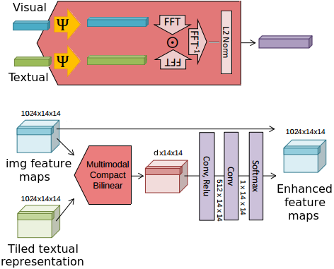
Figure 1: Left: Tensor Sketch algorithm - Right: Compact Bilinear Pooling for two modality vectors (top) and ”MM pre-attention” model (bottom) ; Note that the textual representation vector is tiled (copied) to match the dimension of the image feature maps

2 Model

We detail our model build from the attention-based encoder-decoder neural network described by Sutskever et al. (2014) and Bahdanau et al. (2014) implemented in TensorFlow (Abadi et al., 2016). Textual encoder  Given an input sentence $X=(x_{1},x_{2},...,x_{T}),x_{i}\in\mathbb{R}^{E}$ where $T$ is the sentence length and $E$ is the dimension of the word embedding space, a bi-directional LSTM encoder of layer size $L$ produces a set of textual annotation $A^{T}=\{h^{t}_{1},h^{t}_{2},...,h^{t}_{T}\}$ where $h_{i}$ is obtained by concatenating the forward and backward hidden states of the encoder: $h^{t}_{i}=[\overrightarrow{h_{i}};\overleftarrow{h_{i}}],h^{t}_{i}\in\mathbb{R}^{2L}$.
Visual encoder  An image associated to this sentence is fed to a deep residual network, computing convolutional feature maps of dimension $14\times 14\times 1024$. We obtain a set of visual annotations $A^{V}=\{h^{v}_{1},h^{v}_{2},...,h^{v}_{196}\}$ where $h^{v}_{i}\in{R}^{1024}$.

Decoder  The decoder produces an output sentence $Y=(y_{1},y_{2},...,y_{T^{\prime}}),y_{i}\in\mathbb{R}^{E}$ and is initialized by $s_{0}=tanh(W_{init}h^{t}_{T}+b_{init})$ where $h^{t}_{T}$ is the textual encoder’s last state. The next decoder states are obtained as follows:

$$s_{t},o_{t}=LSTM(s_{t-1},W_{in}[y_{t-1};c_{t-1}]),y_{t-1}\in\mathbb{R}^{E}$$ (1)

During training, $y_{t-1}$ is the ground truth symbol in the sentence whilst $c_{t-1}$ is the previous attention vector computed by the attention model. The current attention vector $c_{t}$, concatenated with the LSTM output $o_{t}$, is used to compute a new vector $\tilde{o_{t}}=W_{proj}[o_{t};c_{t}]+b_{proj}$. The probability distribution over the target vocabulary is computed by the equation :

$$p(y_{t}|y_{t-1},s_{t-1},c_{t-1},A^{T},A^{V})=softmax(W_{out}\tilde{o_{t}}+b_{out})$$ (2)

Attention  At every time-step, the attention mechanism computes two modality specific context vectors $\{c^{t}_{t},c^{v}_{t}\}$ given the current decoder state $s_{t}$ and the two annotation sets $\{A^{T},A^{V}\}$. We use the same attention model for both modalities described by Vinyals et al. (2015). We first compute modality specific attention weights $\alpha^{mod}_{t}=softmax(v^{T}tanh(W_{1}A^{mod}+W_{2}s_{t}+b))$. The context vector is then obtained with the following weighted sum : $c_{t}^{mod}=\sum\limits_{i=1}^{\lvert A^{mod}\rvert}\alpha_{ti}^{mod}h_{i}^{mod}$
Both $v^{T}$ and $W_{1}$ are considered modalities dependent and thus aren’t shared by both modalities. The projection layer $W_{2}$ is applied to the decoder state $s_{t}$ and is thus shared (Caglayan et al., 2016). Vectors $\{c^{t}_{t},c^{v}_{t}\}$ are then combined to produce $c_{t}$ with an element-wise (e-w) sum / product or concatenation layer.

Multimodal Compact Bilinear (MCB) pooling  Bilinear models (Tenenbaum & Freeman, 1997) can be applied as vectors combination. We take the outer product of our two context vectors $c^{t}$ and $c^{v}\in\mathbb{R}^{2L}$ then learn a linear model $W$ i.e. $c_{t}=W[c^{t}_{t}\otimes c^{t}_{v}]$, where $\otimes$ denotes the outer product and $[$ $]$ denotes linearizing the matrix in a vector. Bilinear pooling allows all elements of both vectors to interact with each other in a multiplicative way but leads to a high dimensional representation and an infeasible number of parameters to learn in $W$. For two modality context vectors of size $2L=1024$ and an attention size of $d=512$ ($c_{t}\in\mathbb{R}^{512}$), $W$ would have $\approx$ 537 million parameters. We use the compact method proposed by Gao et al. (2016), based on the tensor sketch algorithm (see Algorithm 1), to make bilinear models feasible. This model, referred as the ”MM Attention” in the results section, is illustrated in Figure 1 (top right)

We try a second model inspired by the work of (Fukui et al., 2016). For each spatial grid location in the visual representation, we use MCB pooling to merge the slice of the visual feature with the language representation. As shown at the bottom right of Figure 1, after the pooling we use two convolutional layers to predict attention weights for each grid location. We then apply softmax to produce a new normalized soft attention map. This method can be seen as the removal of unnecessary information in the feature maps according to the source sentence. Note that we still use the ”MM attention” during decoding. We refer this model as the ”MM pre-attention”.

3 Settings

We use the Adam optimizer (Kingma & Ba, 2014) with a l.r. of $\alpha=0.0007$ and L2 regularization of $\delta=10^{-5}$. Layer size $L$ and word embeddings size $E$ is 512. Embeddings are trained along with the model. We use mini-batch size of 32 and Xavier weight initialization (Glorot & Bengio, 2010). For this experiments, we used the Multi30K dataset (Elliott et al., 2016) which is an extended version of the Flickr30K Entities. For each image, one of the English descriptions was selected and manually translated into German by a professional translator (Task 1). As training and development data, 29,000 and 1,014 triples are used respectively. A test set of size 1000 is used for BLEU and METEOR evaluation. Vocabulary sizes are 11,180 (en) and 19,154 (de). We lowercase and tokenize all the text data with the Moses tokenizer. We extract feature maps from the images with a ResNet-50 at its $res4f\_relu$ layer. We use early-stopping if no improvement is observed after 10,000 steps.

4 Results

Table 1: The BLEU and METEOR results on the test split containing 1000 triples. All scores are the average of two runs.

Method	Validation Scores
	BLEU	METEOR
Monomodal Text	29.24	48.32
MM attention
Concatenation	26.12	44.14
Element-wise Sum	27.48	45.79
Element-wise Product	28.62	47.99
MCB 1024	28.48	47.57
MM pre-attention*
Element-wise sum	28.57	46.40
Element-wise Product	29.14	46.71
MCB 4096	29.75	48.80
*with Prod as MM att.

Compact Bilinear $d$	BLEU
Multimodal attention
512	27.78
1024	28.48
2048	28.12
Multimodal pre-attention
1024	28.71
2048	29.19
4096	29.75
8192	29.39
16000	27.98

To our knowledge, there is currently no multimodal translation architecture that convincingly surpass a monomodal NMT baseline. Our work nevertheless shows a small but encouraging improvement. In the ”MM attention” model, where both attention context vectors are merged, we notice no improvement using MCB over an element-wise product. We suppose the reason is that the merged attention vector $c_{t}$ has to be concatenated with the cell output and then gets linearly transformed by the proj layer to a vector of size 512. This heavy dimensionality reduction undergone by the vector may have lead to a consequent loss of information, thus the poor results. This motivated us to implement the second attention mechanism, ”MM pre-attention”. Here, the attention model can enjoy the full use of the combined vectors dimension, varying from 1024 to 16000. We show here an improvement of +0.62 BLEU over e-w multiplication and +1.18 BLEU over e-w sum. We believe a step further could be to investigate different experimental settings or layer architectures as we felt MCB could perform much better as seen in similar previous work (Fukui et al., 2016).

5 Acknowledgements

This work was partly supported by the Chist-Era project IGLU with contribution from the Belgian Fonds de la Recherche Scientique (FNRS), contract no. R.50.11.15.F, and by the FSO project VCYCLE with contribution from the Belgian Waloon Region, contract no. 1510501.

References

- Abadi et al. (2016) Martín Abadi, Ashish Agarwal, Paul Barham, Eugene Brevdo, Zhifeng Chen, Craig Citro, Greg S Corrado, Andy Davis, Jeffrey Dean, Matthieu Devin, et al. Tensorflow: Large-scale machine learning on heterogeneous distributed systems. arXiv preprint arXiv:1603.04467, 2016.
- Bahdanau et al. (2014) Dzmitry Bahdanau, Kyunghyun Cho, and Yoshua Bengio. Neural machine translation by jointly learning to align and translate. arXiv preprint arXiv:1409.0473, 2014.
- Caglayan et al. (2016) Ozan Caglayan, Walid Aransa, Yaxing Wang, Marc Masana, Mercedes García-Martínez, Fethi Bougares, Loïc Barrault, and Joost van de Weijer. Does multimodality help human and machine for translation and image captioning? arXiv preprint arXiv:1605.09186, 2016.
- Calixto et al. (2017) Iacer Calixto, Qun Liu, and Nick Campbell. Doubly-attentive decoder for multi-modal neural machine translation. arXiv preprint arXiv:1702.01287, 2017.
- Elliott et al. (2016) D. Elliott, S. Frank, K. Sima’an, and L. Specia. Multi30k: Multilingual english-german image descriptions. pp. 70–74, 2016.
- Fukui et al. (2016) Akira Fukui, Dong Huk Park, Daylen Yang, Anna Rohrbach, Trevor Darrell, and Marcus Rohrbach. Multimodal compact bilinear pooling for visual question answering and visual grounding. arXiv preprint arXiv:1606.01847, 2016.
- Gao et al. (2016) Yang Gao, Oscar Beijbom, Ning Zhang, and Trevor Darrell. Compact bilinear pooling. In Proceedings of the IEEE Conference on Computer Vision and Pattern Recognition, pp. 317–326, 2016.
- Glorot & Bengio (2010) Xavier Glorot and Yoshua Bengio. Understanding the difficulty of training deep feedforward neural networks. In Aistats, volume 9, pp. 249–256, 2010.
- He et al. (2016) Kaiming He, Xiangyu Zhang, Shaoqing Ren, and Jian Sun. Deep residual learning for image recognition. In The IEEE Conference on Computer Vision and Pattern Recognition (CVPR), June 2016.
- Huang et al. (2016) Po-Yao Huang, Frederick Liu, Sz-Rung Shiang, Jean Oh, and Chris Dyer. Attention-based multimodal neural machine translation. In Proceedings of the First Conference on Machine Translation, Berlin, Germany, 2016.
- Kingma & Ba (2014) Diederik Kingma and Jimmy Ba. Adam: A method for stochastic optimization. arXiv preprint arXiv:1412.6980, 2014.
- Sutskever et al. (2014) Ilya Sutskever, Oriol Vinyals, and Quoc V Le. Sequence to sequence learning with neural networks. In Advances in neural information processing systems, pp. 3104–3112, 2014.
- Tenenbaum & Freeman (1997) Joshua B Tenenbaum and William T Freeman. Separating style and content. Advances in neural information processing systems, pp. 662–668, 1997.
- Vinyals et al. (2015) Oriol Vinyals, Łukasz Kaiser, Terry Koo, Slav Petrov, Ilya Sutskever, and Geoffrey Hinton. Grammar as a foreign language. In Advances in Neural Information Processing Systems, pp. 2773–2781, 2015.
- Xu et al. (2015) Kelvin Xu, Jimmy Ba, Ryan Kiros, Kyunghyun Cho, Aaron C Courville, Ruslan Salakhutdinov, Richard S Zemel, and Yoshua Bengio. Show, attend and tell: Neural image caption generation with visual attention. In ICML, volume 14, pp. 77–81, 2015.