Variational Principles and Applications of Local Topological Constants of Motion for Non-Barotropic Magnetohydrodynamics

Abstract

Variational principles for magnetohydrodynamics (MHD) were introduced by previous authors both in Lagrangian and Eulerian form. In this paper we introduce simpler Eulerian variational principles from which all the relevant equations of non-barotropic MHD can be derived for certain field topologies. The variational principle is given in terms of five independent functions for non-stationary non-barotropic flows. This is less then the eight variables which appear in the standard equations of barotropic MHD which are the magnetic field $\vec{B}$ the velocity field $\vec{v}$, the entropy $s$ and the density $\rho$.

The case of non-barotropic MHD in which the internal energy is a function of both entropy and density was not discussed in previous works which were concerned with the simplistic barotropic case. It is important to understand the rule of entropy and temperature for the variational analysis of MHD. Thus we introduce a variational principle of non-barotropic MHD and show that five functions will suffice to describe this physical system.

We will also discuss the implications of the above analysis for topological constants. It will be shown that while cross helicity is not conserved for non-barotropic MHD a variant of this quantity is. The implications of this to non-barotropic MHD stability is discussed.

Keywords: Magnetohydrodynamics, Variational principles, Topological conservation laws

PACS number(s): 47.65.+a

• December 2016

1 Introduction

Cross Helicity was first described by Woltjer [2, 3] and is give by:

$$H_{C}\equiv\int\vec{B}\cdot\vec{v}d^{3}x,$$ (1)

in which $\vec{B}$ is the magnetic field, $\vec{v}$ is the velocity field and the integral is taken over the entire flow domain. $H_{C}$ is conserved for barotropic or incompressible MHD and is given a topological interpretation in terms of the knottiness of magnetic and flow field lines. An analogous conserved helicity for fluid dynamics was obtained by Moffatt [16]. A generalization of barotropic fluid dynamics conserved quantities including helicity to non barotropic flows including topological constants of motion is given by Mobbs [4]. However, Mobbs did not discuss the MHD case.

Both conservation laws for the helicity in the fluid dynamics case and the barotropic MHD case were shown to originate from a relabelling symmetry through the Noether theorem [6, 7, 8, 9]. Webb et al. [11] have generalized the idea of relabelling symmetry to non-barotropic MHD and derived their generalized cross helicity conservation law by using Noether s theorem. The conservation law deduction involves a divergence symmetry of the action. These conservation laws were written as Eulerian conservation laws of the form $D_{t}+\vec{\nabla}\cdot\vec{F}=0$ where D is the conserved density and F is the conserved flux. Webb et al. [13] discuss the cross helicity conservation law for non-barotropic MHD in a multi-symplectic formulation of MHD. Webb et al. [10, 11] emphasize that the generalized cross helicity conservation law, in MHD and the generalized helicity conservation law in non-barotropic fluids are non-local in the sense that they depend on the auxiliary nonlocal variable $\sigma$, which depends on the Lagrangian time integral of the temperature $T(x,t)$. Notice that a potential vorticity conservation equation for non-barotropic MHD is derived by Webb, G. M. and Mace, R.L. [14] by using Noether s second theorem.

It should be mentioned that Mobbs [4] derived a helicity conservation law for ideal, non-barotropic fluid dynamics, which is of the same form as the cross helicity conservation law for non-barotropic MHD, except that the magnetic field induction is replaced by the generalized fluid helicity $\vec{\Omega}=\vec{\nabla}\times(\vec{v}-\sigma\vec{\nabla}s)$. Webb et al. [10, 11] also derive the Eulerian, differential form of Mobbs [4] conservation law (although they did not reference Mobbs [4]). Webb and Anco [12] show how Mobbs conservation law arises in multi-symplectic, Lagrangian fluid mechanics.

Variational principles for MHD were introduced by previous authors both in Lagrangian and Eulerian form. Sturrock [15] has discussed in his book a Lagrangian variational formalism for MHD. Vladimirov and Moffatt [16] in a series of papers have discussed an Eulerian variational principle for incompressible MHD. However, their variational principle contained three more functions in addition to the seven variables which appear in the standard equations of incompressible MHD which are the magnetic field $\vec{B}$ the velocity field $\vec{v}$ and the pressure $P$. Kats [17] has generalized Moffatt’s work for compressible non barotropic flows but without reducing the number of functions and the computational load. Moreover, Kats has shown that the variables he suggested can be utilized to describe the motion of arbitrary discontinuity surfaces [18, 19]. Sakurai [20] has introduced a two function Eulerian variational principle for force-free MHD and used it as a basis of a numerical scheme, his method is discussed in a book by Sturrock [15]. A method of solving the equations for those two variables was introduced by Yang, Sturrock & Antiochos [22]. Yahalom & Lynden-Bell [9] combined the Lagrangian of Sturrock [15] with the Lagrangian of Sakurai [20] to obtain an Eulerian Lagrangian principle for barotropic MHD which will depend on only six functions. The variational derivative of this Lagrangian produced all the equations needed to describe barotropic MHD without any additional constraints. The equations obtained resembled the equations of Frenkel, Levich & Stilman [29] (see also [30]). Yahalom [23] have shown that for the barotropic case four functions will suffice. Moreover, it was shown that the cuts of some of those functions [24] are topological local conserved quantities.

Variational principles of non barotropic MHD can be found in the work of Bekenstein & Oron [31] in terms of 15 functions and V.A. Kats [17] in terms of 20 functions. The author of this paper suspect that this number can be somewhat reduced. Moreover, A. V. Kats in a remarkable paper [32] (section IV,E) has shown that there is a large symmetry group (gauge freedom) associated with the choice of those functions, this implies that the number of degrees of freedom can be reduced. Here we will show that only five functions will suffice to describe non barotropic MHD in the case that we enforce a Sakurai [20] representation for the magnetic field. Morrison [21] has suggested a Hamiltonian approach but this also depends on 8 canonical variables (see table 2 [21]). In a series of papers Yahalom has suggest a five function variational principle for non-barotropic MHD [25, 26, 27, 28]

The plan of this paper is as follows: First we introduce the standard notations and equations of non-barotropic MHD. Next we introduce a generalization of the barotropic variational principle suitable for the non-barotropic case. Later we simplify the Eulerian variational principle and formulate it in terms of eight functions. Next we show how three variational variables can be integrated algebraically thus reducing the variational principle to five functions. Then we discuss the Aharanov-Bohm effect and analogous phenomena in non-barotropic MHD which are related to the topological conservation laws of magnetic helicity and non-barotropic cross helicity. Finally we discuss the application of those to the stability of MHD flows.

2 Standard formulation of non-barotropic magnetohydrodynamics

The standard set of equations solved for non-barotropic MHD are given below:

$$\frac{\partial{\vec{B}}}{\partial t}=\vec{\nabla}\times(\vec{v}\times\vec{B}),$$ (2)

$$\vec{\nabla}\cdot\vec{B}=0,$$ (3)

$$\frac{\partial{\rho}}{\partial t}+\vec{\nabla}\cdot(\rho\vec{v})=0,$$ (4)

$$\rho\frac{d\vec{v}}{dt}=\rho(\frac{\partial\vec{v}}{\partial t}+(\vec{v}\cdot\vec{\nabla})\vec{v})=-\vec{\nabla}p(\rho,s)+\frac{(\vec{\nabla}\times\vec{B})\times\vec{B}}{4\pi}.$$ (5)

$$\frac{ds}{dt}=0.$$ (6)

The following notations are utilized: $\frac{\partial}{\partial t}$ is the temporal derivative, $\frac{d}{dt}$ is the temporal material derivative and $\vec{\nabla}$ has its standard meaning in vector calculus. $\vec{B}$ is the magnetic field vector, $\vec{v}$ is the velocity field vector, $\rho$ is the fluid density and $s$ is the specific entropy. Finally $p(\rho,s)$ is the pressure which depends on the density and entropy (the non-barotropic case).

The justification for those equations and the conditions under which they apply can be found in standard books on MHD (see for example [15]). The above applies to a collision-dominated plasma in local thermodynamic equilibrium. Such conditions are seldom satisfied by physical plasmas, certainly not in astrophysics or in fusion-relevant magnetic confinement experiments. Never the less it is believed that the fastest macroscopic instabilities in those systems obey the above equations [24], while instabilities associated with viscous or finite conductivity terms are slower. It should be noted that due to a theorem by Bateman [34] every physical system can be described by a variational principle (including viscous plasma) the trick is to find an elegant variational principle usually depending on a small amount of variational variables. The current work will discuss only ideal MHD while viscous MHD will be left for future endeavors.

Equation (2) describes the fact that the magnetic field lines are moving with the fluid elements (”frozen” magnetic field lines), equation (3) describes the fact that the magnetic field is solenoidal, equation (4) describes the conservation of mass and equation (5) is the Euler equation for a fluid in which both pressure and Lorentz magnetic forces apply. The term:

$$\vec{J}=\frac{\vec{\nabla}\times\vec{B}}{4\pi},$$ (7)

is the electric current density which is not connected to any mass flow. Equation (6) describes the fact that heat is not created (zero viscosity, zero resistivity) in ideal non-barotropic MHD and is not conducted, thus only convection occurs. The number of independent variables for which one needs to solve is eight ($\vec{v},\vec{B},\rho,s$) and the number of equations (2,4,5,6) is also eight. Notice that equation (3) is a condition on the initial $\vec{B}$ field and is satisfied automatically for any other time due to equation (2).

3 Variational principle of non-barotropic magnetohydrodynamics

In the following section we will generalize the approach of [9] for the non-barotropic case. Consider the action:

$$A \equiv \int{\cal L}d^{3}xdt,$$

$${\cal L} \equiv {\cal L}_{1}+{\cal L}_{2},$$

$${\cal L}_{1} \equiv \rho(\frac{1}{2}\vec{v}^{2}-\varepsilon(\rho,s))+\frac{\vec{B}^{2}}{8\pi},$$

$${\cal L}_{2} \equiv \nu[\frac{\partial{\rho}}{\partial t}+\vec{\nabla}\cdot(\rho\vec{v})]-\rho\alpha\frac{d\chi}{dt}-\rho\beta\frac{d\eta}{dt}-\rho\sigma\frac{ds}{dt}-\frac{\vec{B}}{4\pi}\cdot\vec{\nabla}\chi\times\vec{\nabla}\eta.$$ (8)

In the above $\varepsilon$ is the specific internal energy (internal energy per unit of mass). The reader is reminded of the following thermodynamic relations which will become useful later:

$$d\varepsilon = Tds-Pd\frac{1}{\rho}=Tds+\frac{P}{\rho^{2}}d\rho$$

$$\frac{\partial\varepsilon}{\partial s}=T,\qquad\frac{\partial\varepsilon}{\partial\rho}=\frac{P}{\rho^{2}}$$

$$w = \varepsilon+\frac{P}{\rho}=\varepsilon+\frac{\partial\varepsilon}{\partial\rho}\rho=\frac{\partial(\rho\varepsilon)}{\partial\rho}$$

$$dw = d\varepsilon+d(\frac{P}{\rho})=Tds+\frac{1}{\rho}dP$$ (9)

in the above $T$ is the temperature and $w$ is the specific enthalpy. Obviously $\nu,\alpha,\beta,\sigma$ are Lagrange multipliers which were inserted in such a way that the variational principle will yield the following equations:

$$\frac{\partial{\rho}}{\partial t}+\vec{\nabla}\cdot(\rho\vec{v})=0,$$

$$\rho\frac{d\chi}{dt}=0,$$

$$\rho\frac{d\eta}{dt}=0.$$

$$\rho\frac{ds}{dt}=0.$$ (10)

It is not assumed that $\nu,\alpha,\beta,\sigma$ are single valued. Provided $\rho$ is not null those are just the continuity equation (4), entropy conservation and the conditions that Sakurai’s functions are comoving. Taking the variational derivative with respect to $\vec{B}$ we see that

$$\vec{B}=\hat{\vec{B}}\equiv\vec{\nabla}\chi\times\vec{\nabla}\eta.$$ (11)

Hence $\vec{B}$ is in Sakurai’s form and satisfies equation (3). It can be easily shown that provided that $\vec{B}$ is in the form given in equation (11), and equations (10) are satisfied, then also equation (2) is satisfied.

For the time being we have showed that all the equations of non-barotropic MHD can be obtained from the above variational principle except Euler’s equations. We will now show that Euler’s equations can be derived from the above variational principle as well. Let us take an arbitrary variational derivative of the above action with respect to $\vec{v}$, this will result in:

$$\delta_{\vec{v}}A=\int dt\{\int d^{3}xdt\rho\delta\vec{v}\cdot[\vec{v}-\vec{\nabla}\nu-\alpha\vec{\nabla}\chi-\beta\vec{\nabla}\eta-\sigma\vec{\nabla}s]+\oint d\vec{S}\cdot\delta\vec{v}\rho\nu+\int d\vec{\Sigma}\cdot\delta\vec{v}\rho[\nu]\}.$$ (12)

The integral $\oint d\vec{S}\cdot\delta\vec{v}\rho\nu$ vanishes in many physical scenarios. In the case of astrophysical flows this integral will vanish since $\rho=0$ on the flow boundary, in the case of a fluid contained in a vessel no flux boundary conditions $\delta\vec{v}\cdot\hat{n}=0$ are induced ($\hat{n}$ is a unit vector normal to the boundary). The surface integral $\int d\vec{\Sigma}$ on the cut of $\nu$ vanishes in the case that $\nu$ is single valued and $[\nu]=0$ as is the case for some flow topologies. In the case that $\nu$ is not single valued only a Kutta type velocity perturbation [33] in which the velocity perturbation is parallel to the cut will cause the cut integral to vanish. An arbitrary velocity perturbation on the cut will indicate that $\rho=0$ on this surface which is contradictory to the fact that a cut surface is to some degree arbitrary as is the case for the zero line of an azimuthal angle. We will show later that the ”cut” surface is co-moving with the flow hence it may become quite complicated. This uneasy situation may be somewhat be less restrictive when the flow has some symmetry properties.

Provided that the surface integrals do vanish and that $\delta_{\vec{v}}A=0$ for an arbitrary velocity perturbation we see that $\vec{v}$ must have the following form:

$$\vec{v}=\hat{\vec{v}}\equiv\vec{\nabla}\nu+\alpha\vec{\nabla}\chi+\beta\vec{\nabla}\eta+\sigma\vec{\nabla}s.$$ (13)

The above equation is reminiscent of Clebsch representation in non magnetic fluids [35, 36]. Let us now take the variational derivative with respect to the density $\rho$ we obtain:

$$\delta_{\rho}A = \int d^{3}xdt\delta\rho[\frac{1}{2}\vec{v}^{2}-w-\frac{\partial{\nu}}{\partial t}-\vec{v}\cdot\vec{\nabla}\nu]$$ (14)

$$+ \int dt\oint d\vec{S}\cdot\vec{v}\delta\rho\nu+\int dt\int d\vec{\Sigma}\cdot\vec{v}\delta\rho[\nu]+\int d^{3}x\nu\delta\rho|^{t_{1}}_{t_{0}}.$$

In which $w=\frac{\partial(\varepsilon\rho)}{\partial\rho}$ is the specific enthalpy. Hence provided that $\oint d\vec{S}\cdot\vec{v}\delta\rho\nu$ vanishes on the boundary of the domain and $\int d\vec{\Sigma}\cdot\vec{v}\delta\rho[\nu]$ vanishes on the cut of $\nu$ in the case that $\nu$ is not single valued and in initial and final times the following equation must be satisfied:

$$\frac{d\nu}{dt}=\frac{1}{2}\vec{v}^{2}-w,\qquad$$ (15)

Since the right hand side of the above equation is single valued as it is made of physical quantities, we conclude that:

$$\frac{d[\nu]}{dt}=0.$$ (16)

Hence the cut value is co-moving with the flow and thus the cut surface may become arbitrary complicated. This uneasy situation may be somewhat be less restrictive when the flow has some symmetry properties.

Finally we have to calculate the variation with respect to both $\chi$ and $\eta$ this will lead us to the following results:

$$\delta_{\chi}A = \int d^{3}xdt\delta\chi[\frac{\partial{(\rho\alpha)}}{\partial t}+\vec{\nabla}\cdot(\rho\alpha\vec{v})-\vec{\nabla}\eta\cdot\vec{J}]+\int dt\oint d\vec{S}\cdot[\frac{\vec{B}}{4\pi}\times\vec{\nabla}\eta-\vec{v}\rho\alpha]\delta\chi$$ (17)

$$+ \int dt\int d\vec{\Sigma}\cdot[\frac{\vec{B}}{4\pi}\times\vec{\nabla}\eta-\vec{v}\rho\alpha][\delta\chi]-\int d^{3}x\rho\alpha\delta\chi|^{t_{1}}_{t_{0}},$$

$$\delta_{\eta}A = \int d^{3}xdt\delta\eta[\frac{\partial{(\rho\beta)}}{\partial t}+\vec{\nabla}\cdot(\rho\beta\vec{v})+\vec{\nabla}\chi\cdot\vec{J}]+\int dt\oint d\vec{S}\cdot[\vec{\nabla}\chi\times\frac{\vec{B}}{4\pi}-\vec{v}\rho\beta]\delta\eta$$ (18)

$$+ \int dt\int d\vec{\Sigma}\cdot[\vec{\nabla}\chi\times\frac{\vec{B}}{4\pi}-\vec{v}\rho\beta][\delta\eta]-\int d^{3}x\rho\beta\delta\eta|^{t_{1}}_{t_{0}}.$$

Provided that the correct temporal and boundary conditions are met with respect to the variations $\delta\chi$ and $\delta\eta$ on the domain boundary and on the cuts in the case that some (or all) of the relevant functions are non single valued. we obtain the following set of equations:

$$\frac{d\alpha}{dt}=\frac{\vec{\nabla}\eta\cdot\vec{J}}{\rho},\qquad\frac{d\beta}{dt}=-\frac{\vec{\nabla}\chi\cdot\vec{J}}{\rho},$$ (19)

in which the continuity equation (4) was taken into account. By correct temporal conditions we mean that both $\delta\eta$ and $\delta\chi$ vanish at initial and final times. As for boundary conditions which are sufficient to make the boundary term vanish on can consider the case that the boundary is at infinity and both $\vec{B}$ and $\rho$ vanish. Another possibility is that the boundary is impermeable and perfectly conducting. A sufficient condition for the integral over the ”cuts” to vanish is to use variations $\delta\eta$ and $\delta\chi$ which are single valued. It can be shown that $\chi$ can always be taken to be single valued, hence taking $\delta\chi$ to be single valued is no restriction at all. In some topologies $\eta$ is not single valued and in those cases a single valued restriction on $\delta\eta$ is sufficient to make the cut term null.

Finally we take a variational derivative with respect to the entropy $s$:

$$\delta_{s}A = \int d^{3}xdt\delta s[\frac{\partial{(\rho\sigma)}}{\partial t}+\vec{\nabla}\cdot(\rho\sigma\vec{v})-\rho T]+\int dt\oint d\vec{S}\cdot\rho\sigma\vec{v}\delta s$$ (20)

$$- \int d^{3}x\rho\sigma\delta s|^{t_{1}}_{t_{0}},$$

in which the temperature is $T=\frac{\partial\varepsilon}{\partial s}$. We notice that according to equation (13) $\sigma$ is single valued and hence no cuts are needed. Taking into account the continuity equation (4) we obtain for locations in which the density $\rho$ is not null the result:

$$\frac{d\sigma}{dt}=T,$$ (21)

provided that $\delta_{s}A$ vanished for an arbitrary $\delta s$.

4 Euler’s equations

We shall now show that a velocity field given by equation (13), such that the equations for $\alpha,\beta,\chi,\eta,\nu,\sigma,s$ satisfy the corresponding equations (10,15,19,21) must satisfy Euler’s equations. Let us calculate the material derivative of $\vec{v}$:

$$\frac{d\vec{v}}{dt}=\frac{d\vec{\nabla}\nu}{dt}+\frac{d\alpha}{dt}\vec{\nabla}\chi+\alpha\frac{d\vec{\nabla}\chi}{dt}+\frac{d\beta}{dt}\vec{\nabla}\eta+\beta\frac{d\vec{\nabla}\eta}{dt}+\frac{d\sigma}{dt}\vec{\nabla}s+\sigma\frac{d\vec{\nabla}s}{dt}.$$ (22)

It can be easily shown that:

$$\frac{d\vec{\nabla}\nu}{dt} = \vec{\nabla}\frac{d\nu}{dt}-\vec{\nabla}v_{k}\frac{\partial\nu}{\partial x_{k}}=\vec{\nabla}(\frac{1}{2}\vec{v}^{2}-w)-\vec{\nabla}v_{k}\frac{\partial\nu}{\partial x_{k}},$$

$$\frac{d\vec{\nabla}\eta}{dt} = \vec{\nabla}\frac{d\eta}{dt}-\vec{\nabla}v_{k}\frac{\partial\eta}{\partial x_{k}}=-\vec{\nabla}v_{k}\frac{\partial\eta}{\partial x_{k}},$$

$$\frac{d\vec{\nabla}\chi}{dt} = \vec{\nabla}\frac{d\chi}{dt}-\vec{\nabla}v_{k}\frac{\partial\chi}{\partial x_{k}}=-\vec{\nabla}v_{k}\frac{\partial\chi}{\partial x_{k}},$$

$$\frac{d\vec{\nabla}s}{dt} = \vec{\nabla}\frac{ds}{dt}-\vec{\nabla}v_{k}\frac{\partial s}{\partial x_{k}}=-\vec{\nabla}v_{k}\frac{\partial s}{\partial x_{k}}.$$ (23)

In which $x_{k}$ is a Cartesian coordinate and a summation convention is assumed. Inserting the result from equations (23,10) into equation (22) yields:

$$\frac{d\vec{v}}{dt} = -\vec{\nabla}v_{k}(\frac{\partial\nu}{\partial x_{k}}+\alpha\frac{\partial\chi}{\partial x_{k}}+\beta\frac{\partial\eta}{\partial x_{k}}+\sigma\frac{\partial s}{\partial x_{k}})+\vec{\nabla}(\frac{1}{2}\vec{v}^{2}-w)+T\vec{\nabla}s$$ (24)

$$+ \frac{1}{\rho}((\vec{\nabla}\eta\cdot\vec{J})\vec{\nabla}\chi-(\vec{\nabla}\chi\cdot\vec{J})\vec{\nabla}\eta)$$

$$= -\vec{\nabla}v_{k}v_{k}+\vec{\nabla}(\frac{1}{2}\vec{v}^{2}-w)+T\vec{\nabla}s+\frac{1}{\rho}\vec{J}\times(\vec{\nabla}\chi\times\vec{\nabla}\eta)$$

$$= -\frac{\vec{\nabla}p}{\rho}+\frac{1}{\rho}\vec{J}\times\vec{B}.$$

In which we have used both equation (13) and equation (11) in the above derivation. This of course proves that the non-barotropic Euler equations can be derived from the action given in equation (8) and hence all the equations of non-barotropic MHD can be derived from the above action without restricting the variations in any way except on the relevant boundaries and cuts.

5 Simplified action

The reader of this paper might argue here that the paper is misleading. The author has declared that he is going to present a simplified action for non-barotropic MHD instead he added six more functions $\alpha,\beta,\chi,\-\eta,\nu,\sigma$ to the standard set $\vec{B},\vec{v},\rho,s$. In the following I will show that this is not so and the action given in equation (8) in a form suitable for a pedagogic presentation can indeed be simplified. It is easy to show that the Lagrangian density appearing in equation (8) can be written in the form:

$${\cal L} = -\rho[\frac{\partial{\nu}}{\partial t}+\alpha\frac{\partial{\chi}}{\partial t}+\beta\frac{\partial{\eta}}{\partial t}+\sigma\frac{\partial{s}}{\partial t}+\varepsilon(\rho,s)]+\frac{1}{2}\rho[(\vec{v}-\hat{\vec{v}})^{2}-(\hat{\vec{v}})^{2}]$$ (25)

$$+ \frac{1}{8\pi}[(\vec{B}-\hat{\vec{B}})^{2}-(\hat{\vec{B}})^{2}]+\frac{\partial{(\nu\rho)}}{\partial t}+\vec{\nabla}\cdot(\nu\rho\vec{v}).$$

In which $\hat{\vec{v}}$ is a shorthand notation for $\vec{\nabla}\nu+\alpha\vec{\nabla}\chi+\beta\vec{\nabla}\eta+\sigma\vec{\nabla}s$ (see equation (13)) and $\hat{\vec{B}}$ is a shorthand notation for $\vec{\nabla}\chi\times\vec{\nabla}\eta$ (see equation (11)). Thus ${\cal L}$ has four contributions:

$${\cal L} = \hat{\cal L}+{\cal L}_{\vec{v}}+{\cal L}_{\vec{B}}+{\cal L}_{boundary},$$

$$\hat{\cal L} \equiv -\rho\left[\frac{\partial{\nu}}{\partial t}+\alpha\frac{\partial{\chi}}{\partial t}+\beta\frac{\partial{\eta}}{\partial t}+\sigma\frac{\partial{s}}{\partial t}+\varepsilon(\rho,s)+\frac{1}{2}(\vec{\nabla}\nu+\alpha\vec{\nabla}\chi+\beta\vec{\nabla}\eta+\sigma\vec{\nabla}s)^{2}\right]$$

$$- \frac{1}{8\pi}(\vec{\nabla}\chi\times\vec{\nabla}\eta)^{2}$$

$${\cal L}_{\vec{v}} \equiv \frac{1}{2}\rho(\vec{v}-\hat{\vec{v}})^{2},$$

$${\cal L}_{\vec{B}} \equiv \frac{1}{8\pi}(\vec{B}-\hat{\vec{B}})^{2},$$

$${\cal L}_{boundary} \equiv \frac{\partial{(\nu\rho)}}{\partial t}+\vec{\nabla}\cdot(\nu\rho\vec{v}).$$ (26)

The only term containing $\vec{v}$ is ${\cal L}_{\vec{v}}$, it can easily be seen that this term will lead, after we nullify the variational derivative with respect to $\vec{v}$, to equation (13) but will otherwise have no contribution to other variational derivatives. Similarly the only term containing $\vec{B}$ is ${\cal L}_{\vec{B}}$ and it can easily be seen that this term will lead, after we nullify the variational derivative, to equation (11) but will have no contribution to other variational derivatives. Also notice that the term ${\cal L}_{boundary}$ contains only complete partial derivatives and thus can not contribute to the equations although it can change the boundary conditions. Hence we see that equations (10), equation (15), equations (19) and equation (21) can be derived using the Lagrangian density:

$$\hat{\cal L}[\alpha,\beta,\chi,\eta,\nu,\rho,\sigma,s]=-\rho[\frac{\partial{\nu}}{\partial t}+\alpha\frac{\partial{\chi}}{\partial t}+\beta\frac{\partial{\eta}}{\partial t}+\sigma\frac{\partial{s}}{\partial t}$$

$$+\ \varepsilon(\rho,s)+\frac{1}{2}(\vec{\nabla}\nu+\alpha\vec{\nabla}\chi+\beta\vec{\nabla}\eta+\sigma\vec{\nabla}s)^{2}]-\frac{1}{8\pi}(\vec{\nabla}\chi\times\vec{\nabla}\eta)^{2}$$ (27)

in which $\hat{\vec{v}}$ replaces $\vec{v}$ and $\hat{\vec{B}}$ replaces $\vec{B}$ in the relevant equations. Furthermore, after integrating the eight equations (10,15,19,21) we can insert the potentials $\alpha,\beta,\chi,\eta,\nu,\sigma,s$ into equations (13) and (11) to obtain the physical quantities $\vec{v}$ and $\vec{B}$. Hence, the general non-barotropic MHD problem is reduced from eight equations (2,4,5,6) and the additional constraint (3) to a problem of eight first order (in the temporal derivative) unconstrained equations. Moreover, the entire set of equations can be derived from the Lagrangian density $\hat{\cal L}$.

6 Further Simplification

6.1 Elimination of Variables

Let us now look at the three last three equations of (10). Those describe three comoving quantities which can be written in terms of the generalized Clebsch form given in equation (13) as follows:

$$\frac{\partial\chi}{\partial t}+(\vec{\nabla}\nu+\alpha\vec{\nabla}\chi+\beta\vec{\nabla}\eta+\sigma\vec{\nabla}s)\cdot\vec{\nabla}\chi=0$$

$$\frac{\partial\eta}{\partial t}+(\vec{\nabla}\nu+\alpha\vec{\nabla}\chi+\beta\vec{\nabla}\eta+\sigma\vec{\nabla}s)\cdot\vec{\nabla}\eta=0$$

$$\frac{\partial s}{\partial t}+(\vec{\nabla}\nu+\alpha\vec{\nabla}\chi+\beta\vec{\nabla}\eta+\sigma\vec{\nabla}s)\cdot\vec{\nabla}s=0$$ (28)

Those are algebraic equations for $\alpha,\beta,\sigma$. Which can be solved such that $\alpha,\beta,\sigma$ can be written as functionals of $\chi,\eta,\nu,s$, resulting eventually in the description of non-barotropic MHD in terms of five functions: $\nu,\rho,\chi,\eta,s$. Let us introduce the notation:

$$\alpha_{i}\equiv(\alpha,\beta,\sigma),\quad\chi_{i}\equiv(\chi,\eta,s),\quad k_{i}\equiv-\frac{\partial\chi_{i}}{\partial t}-\vec{\nabla}\nu\cdot\vec{\nabla}\chi_{i},\qquad i\in(1,2,3)$$ (29)

In terms of the above notation equation (28) takes the form:

$$k_{i}=\alpha_{j}\vec{\nabla}\chi_{i}\cdot\vec{\nabla}\chi_{j},\qquad j\in(1,2,3)$$ (30)

in which the Einstein summation convention is assumed. Let us define the matrix:

$$A_{ij}\equiv\vec{\nabla}\chi_{i}\cdot\vec{\nabla}\chi_{j}$$ (31)

obviously this matrix is symmetric since $A_{ij}=A_{ji}$. Hence equation (30) takes the form:

$$k_{i}=A_{ij}\alpha_{j},\qquad j\in(1,2,3)$$ (32)

Provided that the matrix $A_{ij}$ is not singular it has an inverse $A^{-1}_{ij}$ which can be written as:

$$A^{-1}_{ij}=\left|A\right|^{-1}\left(\begin{array}[]{ccc}A_{22}A_{33}-A_{23}^{2}&A_{13}A_{23}-A_{12}A_{33}&A_{12}A_{23}-A_{13}A_{22}\\ A_{13}A_{23}-A_{12}A_{33}&A_{11}A_{33}-A_{13}^{2}&A_{12}A_{13}-A_{11}A_{23}\\ A_{12}A_{23}-A_{13}A_{22}&A_{12}A_{13}-A_{11}A_{23}&A_{11}A_{22}-A_{12}^{2}\end{array}\right)$$ (33)

In which the determinant $\left|A\right|$ is given by the following equation:

$$\left|A\right|=A_{11}A_{22}A_{33}-A_{11}A_{23}^{2}-A_{22}A_{13}^{2}-A_{33}A_{12}^{2}+2A_{12}A_{13}A_{23}$$ (34)

In terms of the above equations the $\alpha_{i}$’s can be calculated as functionals of $\chi_{i},\nu$ as follows:

$$\alpha_{i}[\chi_{i},\nu]=A^{-1}_{ij}k_{j}.$$ (35)

The velocity equation (13) can now be written as:

$$\vec{v}=\vec{\nabla}\nu+\alpha_{i}\vec{\nabla}\chi_{i}=\vec{\nabla}\nu+A^{-1}_{ij}k_{j}\vec{\nabla}\chi_{i}=\vec{\nabla}\nu-A^{-1}_{ij}\vec{\nabla}\chi_{i}(\frac{\partial\chi_{j}}{\partial t}+\vec{\nabla}\nu\cdot\vec{\nabla}\chi_{j}).$$ (36)

Provided that the $\chi_{i}$ is a coordinate basis in three dimensions, we may write:

$$\vec{\nabla}\nu=\vec{\nabla}\chi_{n}\frac{\partial\nu}{\partial\chi_{n}},\qquad n\in(1,2,3).$$ (37)

Inserting equation (37) into equation (36) we obtain:

$$\vec{v} = -A^{-1}_{ij}\vec{\nabla}\chi_{i}\frac{\partial\chi_{j}}{\partial t}+\vec{\nabla}\nu-A^{-1}_{ij}\vec{\nabla}\chi_{i}\frac{\partial\nu}{\partial\chi_{n}}\vec{\nabla}\chi_{n}\cdot\vec{\nabla}\chi_{j}$$ (38)

$$= -A^{-1}_{ij}\vec{\nabla}\chi_{i}\frac{\partial\chi_{j}}{\partial t}+\vec{\nabla}\nu-A^{-1}_{ij}A_{jn}\vec{\nabla}\chi_{i}\frac{\partial\nu}{\partial\chi_{n}}$$

$$= -A^{-1}_{ij}\vec{\nabla}\chi_{i}\frac{\partial\chi_{j}}{\partial t}+\vec{\nabla}\nu-\delta_{in}\vec{\nabla}\chi_{i}\frac{\partial\nu}{\partial\chi_{n}}$$

$$= -A^{-1}_{ij}\vec{\nabla}\chi_{i}\frac{\partial\chi_{j}}{\partial t}+\vec{\nabla}\nu-\vec{\nabla}\chi_{n}\frac{\partial\nu}{\partial\chi_{n}}$$

$$= -A^{-1}_{ij}\vec{\nabla}\chi_{i}\frac{\partial\chi_{j}}{\partial t}$$

in the above $\delta_{in}$ is a Kronecker delta. Thus the velocity $\vec{v}[\chi_{i}]$ is a functional of $\chi_{i}$ only and is independent of $\nu$.

6.2 Lagrangian Density and Variational Analysis

Let us now rewrite the Lagrangian density $\hat{\cal L}[\chi_{i},\nu,\rho]$ given in equation (27) in terms of the new variables:

$$\hat{\cal L}[\chi_{i},\nu,\rho]=-\rho[\frac{\partial{\nu}}{\partial t}+\alpha_{k}[\chi_{i},\nu]\frac{\partial{\chi_{k}}}{\partial t}+\ \varepsilon(\rho,\chi_{3})+\frac{1}{2}\vec{v}[\chi_{i}]^{2}]-\frac{1}{8\pi}(\vec{\nabla}\chi_{1}\times\vec{\nabla}\chi_{2})^{2}$$ (39)

Let us calculate the variational derivative of $\hat{\cal L}[\chi_{i},\nu,\rho]$ with respect to $\chi_{i}$ this will result in:

$$\delta_{\chi_{i}}\hat{\cal L}=-\rho[\delta_{\chi_{i}}\alpha_{k}\frac{\partial{\chi_{k}}}{\partial t}+\alpha_{\underline{i}}\frac{\partial\delta\chi_{\underline{i}}}{\partial t}+\ \delta_{\chi_{i}}\varepsilon(\rho,\chi_{3})+\delta_{\chi_{i}}\vec{v}\cdot\vec{v}]-\frac{\vec{B}}{4\pi}\cdot\delta_{\chi_{i}}(\vec{\nabla}\chi_{1}\times\vec{\nabla}\chi_{2})$$ (40)

in which the summation convention is not applied if the index is underlined. However, due to equation (36) we may write:

$$\delta_{\chi_{i}}\vec{v}=\delta_{\chi_{i}}\alpha_{k}\vec{\nabla}\chi_{k}+\alpha_{\underline{i}}\vec{\nabla}\delta\chi_{\underline{i}}.$$ (41)

Inserting equation (41) into equation (40) and rearranging the terms we obtain:

$$\delta_{\chi_{i}}\hat{\cal L} = -\rho[\delta_{\chi_{i}}\alpha_{k}(\frac{\partial{\chi_{k}}}{\partial t}+\vec{v}\cdot\vec{\nabla}\chi_{k})+\alpha_{\underline{i}}(\frac{\partial\delta\chi_{\underline{i}}}{\partial t}+\vec{v}\cdot\vec{\nabla}\delta\chi_{\underline{i}})+\ \delta_{\chi_{i}}\varepsilon(\rho,\chi_{3})]$$ (42)

$$- \frac{\vec{B}}{4\pi}\cdot\delta_{\chi_{i}}(\vec{\nabla}\chi_{1}\times\vec{\nabla}\chi_{2}).$$

Now by construction $\vec{v}$ satisfies equation (28) and hence $\frac{\partial{\chi_{k}}}{\partial t}+\vec{v}\cdot\vec{\nabla}\chi_{k}=0$, this leads to:

$$\delta_{\chi_{i}}\hat{\cal L}=-\rho\left[\alpha_{\underline{i}}\frac{d\delta\chi_{\underline{i}}}{dt}+\delta_{\chi_{i}}\varepsilon(\rho,\chi_{3})\right]-\frac{\vec{B}}{4\pi}\cdot\delta_{\chi_{i}}(\vec{\nabla}\chi_{1}\times\vec{\nabla}\chi_{2}).$$ (43)

From now on the derivation proceeds as in equations (17,18,20) resulting in equations (19,21) and will not be repeated. The difference is that now $\alpha,\beta$ and $\sigma$ are not independent quantities, rather they depend through equation (35) on the derivatives of $\chi_{i},\nu$. Thus, equations (17,18,20) are not first order equations in time but are second order equations. Now let us calculate the variational derivative with respect to $\nu$ this will result in the expression:

$$\delta_{\nu}\hat{\cal L}=-\rho[\frac{\partial{\delta\nu}}{\partial t}+\delta_{\nu}\alpha_{n}\frac{\partial{\chi_{n}}}{\partial t}]$$ (44)

However, $\delta_{\nu}\alpha_{k}$ can be calculated from equation (35):

$$\delta_{\nu}\alpha_{n}=A^{-1}_{nj}\delta_{\nu}k_{j}=-A^{-1}_{nj}\vec{\nabla}\delta\nu\cdot\vec{\nabla}\chi_{j}$$ (45)

Inserting the above equation into equation (44):

$$\delta_{\nu}\hat{\cal L}=-\rho[\frac{\partial{\delta\nu}}{\partial t}-A^{-1}_{nj}\vec{\nabla}\chi_{j}\frac{\partial{\chi_{n}}}{\partial t}\cdot\vec{\nabla}\delta\nu]=-\rho[\frac{\partial{\delta\nu}}{\partial t}+\vec{v}\cdot\vec{\nabla}\delta\nu]=-\rho\frac{d{\delta\nu}}{dt}$$ (46)

The above equation can be put to the form:

$$\delta_{\nu}\hat{\cal L}=\delta\nu[\frac{\partial{\rho}}{\partial t}+\vec{\nabla}\cdot(\rho\vec{v})]-\frac{\partial{(\rho\delta\nu)}}{\partial t}-\vec{\nabla}\cdot(\rho\vec{v}\delta\nu)$$ (47)

This obviously leads to the continuity equation (4) and some boundary terms in space and time. The variational derivative with respect to $\rho$ is trivial and the analysis is identical to the one in equation (14) leading to equation (15). To conclude this subsection let us summarize the equations of non-barotropic MHD:

$$\frac{d\nu}{dt} = \frac{1}{2}\vec{v}^{2}-w,$$

$$\frac{\partial{\rho}}{\partial t} + \vec{\nabla}\cdot(\rho\vec{v})=0$$

$$\frac{d\sigma}{dt} = T,$$

$$\frac{d\alpha}{dt} = \frac{\vec{\nabla}\eta\cdot\vec{J}}{\rho},$$

$$\frac{d\beta}{dt} = -\frac{\vec{\nabla}\chi\cdot\vec{J}}{\rho},$$ (48)

in which $\alpha,\beta,\sigma,\vec{v}$ are functionals of $\chi,\eta,s,\nu$ as described above. It is easy to show as in equation (24) that those variational equations are equivalent to the physical equations.

It is shown in [25] tha the Lagrangian density can be written standard quadratic form:

$$\hat{\cal L}[\chi_{i},\nu,\rho]=\rho[\frac{1}{2}A^{-1}_{jn}\frac{\partial\chi_{j}}{\partial t}\frac{\partial\chi_{n}}{\partial t}+\frac{\partial\nu}{\partial\chi_{m}}\frac{\partial{\chi_{m}}}{\partial t}-\frac{\partial{\nu}}{\partial t}-\ \varepsilon(\rho,\chi_{3})]-\frac{1}{8\pi}(\vec{\nabla}\chi_{1}\times\vec{\nabla}\chi_{2})^{2}.$$ (49)

In which $A^{-1}_{jn}$ plays the rule of a ”metric”. The Lagrangian is thus composed of a kinetic terms which is quadratic in the temporal derivatives, a ”gyroscopic” terms which is linear in the temporal derivative and a potential term which is independent of the temporal derivative.

7 The Aharonov-Bohm Effect

Consider an electron moving from A to B (figure 1) in the middle we have a magnetic field $\vec{B}$ going into the plane through which the electron is forbidden to pass, hence for the electron the magnetic field is zero. However, the vector potential $\vec{A}$ is not zero, in fact:

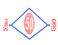
Figure 1: An electron is moving from point A to point B. In the middle of the figure we have a confined magnetic field of 50 Tesla.

$$\vec{B}=\vec{\nabla}\times\vec{A}=0\Rightarrow\vec{A}=\vec{\nabla}\bar{S}$$ (50)

$\vec{\nabla}$ has its standard meaning in vector calculus, $\bar{S}$ is a non single valued function and its discontinuous variation in value (which we shall call discontinuity in the following) $[\bar{S}]$ can be calculated immediately using Stokes theorem:

$$\Phi=\int\vec{B}\cdot d\vec{S}=\int\vec{\nabla}\times\vec{A}\cdot d\vec{S}=\oint\vec{A}\cdot d\vec{l}=\oint\vec{\nabla}\bar{S}\cdot d\vec{l}=[\bar{S}]$$ (51)

Here $\Phi$ is the magnetic flux, the first integral is an area integral and the third is a line integral in which the trajectory goes around the confined magnetic field. Aharonov and Bohm [38] have shown that $\bar{S}$ is proportional to the phase of the electron wave function. Thus its discontinuity will cause interference at point B. If the magnetic field is uniform in a cylinder and zero outside the cylinder, the vector potential can be calculated to be:

$$\vec{A}=A_{\theta}\hat{\theta}=\frac{\Phi}{2\pi\,r}\hat{\theta}\,=\vec{\nabla}\bar{S}\Rightarrow\bar{S}=\frac{\Phi}{2\pi\,}\theta+\bar{S}_{0}.$$ (52)

Where $\theta$ is the azimuthal angle.

Figure 2: The azimuth-radius coordinate system, used to calculate the vector potential. The magnetic field vanishes except at the gray area.

The main features of the Aharonov - Bohm effect are:

1. A domain that is not simply connected due to the presence of a magnetic field, but can be made simply connected by introducing a cut. Mathematically speaking the domain has a non-trivial fundamental Homotopy group. Two classes of loops exist in the plane; loops that can be contracted to a point without intersecting the magnetic region and loops that can not.

2. The electron (or its wave function) do not feel directly the magnetic field – non locality.

3. The potential vector field is a gradient of a non-single valued function.

4. Gauge freedom is not gone but only limited to single-valued gauges.

The discontinuity $[\bar{S}]$ causes a phase difference of the form $2\pi\frac{e}{ch}[\bar{S}]$ between the electron’s ”trajectories”. It will be shown later that the analogous quantity in MHD do not cause such an effect. However, it will lead to a new constant of motion of MHD which is the cross helicity per unit of magnetic flux. It should also be mentioned that according to Bohm’s causal interpretation of quantum mechanics there is a quantum - classical correspondence. According to Bohm [44, 45] the phase of a wave function $S$ should be interpreted as a potential of the velocity field $\vec{v}$:

$$\vec{v}=\frac{1}{m}\vec{\nabla}S$$ (53)

$m$ is the mass of the particle. However, this correspondence can go the other way around! If the velocity field has a potential part it can be interpreted as a phase of a wave function. It will be shown that this potential function has the topological properties somewhat analogous to a phase even if the wave function does not exist in the theory under study.

Earlier classical analogues to the Aharonov - Bohm effect were discussed by Berry et al. [41] which describes a classical analogue to the AB effect in surface waves of swirling water. Never the less I would like to highlight the major differences between the approach of Berry et al. and the approach to be described below. First in the current paper the classical analogue is related to magnetohydrodynamics while in Berry et al. it is related to non magnetic fluids. Second, in the current work one does not assume small perturbations (”waves”) but rather to results that are valid for any ideal MHD flow. Third one does not assume a ”slow change” as in Berry et al. paper in which the velocity field is assumed small with respect to the group velocity; in the current work the results are correct for any rate of change. Fourth the classical analogue of Berry et al. is not related to any vector potential or magnetic flux but they show that a velocity field can play the same rule of a vector potential for surface waves interacting with such a velocity field. Fifth, the current AB effects are related to topological conservation laws in MHD, while there is no such a relation in [41].

8 Topological Constants of Motion

Magnetohydrodynamics is known to have the following two topological constants of motion; one is the magnetic helicity:

$$H_{M}\equiv\int\vec{B}\cdot\vec{A}d^{3}x,$$ (54)

which is known to measure the degree of knottiness of lines of the magnetic field $\vec{B}$ [2, 3]. The domain of integration in equation (54) is the entire space, obviously regions containing a null magnetic field will have a null contribution to the integral. In the above equation $\vec{A}$ is the vector potential defined implicitly by equation (50). The other topological constant is the magnetic cross helicity:

$$H_{C}\equiv\int\vec{B}\cdot\vec{v}d^{3}x,$$ (55)

characterizing the degree of cross knottiness of the magnetic field and vortex lines. The domain of integration in equation (1) is the magnetohydrodynamic flow domain. As noticed before this second topological constant of motion is only constant for barotropic or incompressible MHD. Notice that in non-barotropic MHD:

$$\frac{dH_{C}}{dt}=\int T\vec{\nabla}S\cdot\vec{B}d^{3}x,$$ (56)

hence generally speaking cross helicity is not conserved.

9 Non-Barotropic Cross Helicity

A clue on how to define cross helicity for non-barotropic MHD can be obtained from the variational analysis described in the previous sections.

Let us now write the cross helicity given in equation (1) in terms of equation (11) and equation (13), this will take the form:

$$H_{C}=\int d\Phi[\nu]+\int d\Phi\oint\sigma ds$$ (57)

in which: $d\Phi=\vec{B}\cdot d\vec{S}=\vec{\nabla}\chi\times\vec{\nabla}\eta\cdot d\vec{S}=d\chi\,d\eta$ and the closed line integral is taken along a magnetic field line. $d\Phi$ is a magnetic flux element which is comoving according to equation (2) and $d\vec{S}$ is an infinitesimal area element. Although the cross helicity is not conserved for non-barotropic flows, looking at the right hand side we see that it is made of a sum of two terms. One which is conserved as both $d\Phi$ and $[\nu]$ are comoving (see equation (16)) and one which is not. This suggests the following definition for the non barotropic cross helicity $H_{CNB}$:

$$H_{CNB}\equiv\int d\Phi[\nu]=H_{C}-\int d\Phi\oint\sigma ds$$ (58)

Which can be written in a more conventional form:

$$H_{CNB}=\int\vec{B}\cdot\vec{v}_{t}d^{3}x$$ (59)

where the topological velocity field is defined as follows:

$$\vec{v}_{t}\equiv\vec{v}-\sigma\vec{\nabla}s$$ (60)

It should be noticed that $H_{CNB}$ is conserved even for an MHD not satisfying the Sakurai topological constraint given in equation (11), provided that we have a field $\sigma$ satisfying the equation $\frac{d\sigma}{dt}=T$. Thus the non barotropic cross helicity conservation law:

$$\frac{dH_{CNB}}{dt}=0,$$ (61)

is more general than the variational principle described by equation (49) as follows from a direct computation using equations (2,4,5,6). Also notice that for a constant specific entropy $S$ we obtain $H_{CNB}=H_{C}$ and the non-barotropic cross helicity reduces to the standard barotropic cross helicity. To conclude we introduce also a local topological conservation law in the spirit of [24] which is the non barotropic cross helicity per unit of magnetic flux. This quantity which is equal to the discontinuity of $\nu$ is conserved and can be written as a sum of the barotropic cross helicity per unit flux and the closed line integral of $sd\sigma$ along a magnetic field line:

$$[\nu]=\frac{dH_{CNB}}{d\Phi}=\frac{dH_{C}}{d\Phi}+\oint sd\sigma.$$ (62)

10 Local Cross Helicities

Let us write the topological constants given in equation (54) and equation (1) in terms of the magnetohydrodynamic potentials $\chi,\eta,\nu,\rho$ introduced in previous sections. First let us combine equation (50) with equation (11) to obtain the equation:

$$\vec{\nabla}\times(\vec{A}-\chi\vec{\nabla}\eta)=0,$$ (63)

this leads immediately to the result:

$$\vec{A}=\chi\vec{\nabla}\eta+\vec{\nabla}\zeta,$$ (64)

in which $\zeta$ is some function. Let us now calculate the scalar product $\vec{B}\cdot\vec{A}$:

$$\vec{B}\cdot\vec{A}=(\vec{\nabla}\chi\times\vec{\nabla}\eta)\cdot\vec{\nabla}\zeta.$$ (65)

We can define a local vector basis: $(\vec{\nabla}\chi,\vec{\nabla}\eta,\vec{\nabla}\mu)$ based on the magnetic field lines. Here, in addition to $\chi,\eta$, we have added another coordinate the magnetic metage $\mu$ which parameterizes the distance along the magnetic field lines [9]. $\vec{\nabla}\zeta$ can thus be written as:

$$\vec{\nabla}\zeta=\frac{\partial\zeta}{\partial\chi}\vec{\nabla}\chi+\frac{\partial\zeta}{\partial\mu}\vec{\nabla}\mu+\frac{\partial\zeta}{\partial\eta}\vec{\nabla}\eta.$$ (66)

Hence we can write:

$$\vec{B}\cdot\vec{A}=\frac{\partial\zeta}{\partial\mu}(\vec{\nabla}\chi\times\vec{\nabla}\eta)\cdot\vec{\nabla}\mu=\frac{\partial\zeta}{\partial\mu}\left|\frac{\partial(\chi,\eta,\mu)}{\partial(x,y,z)}\right|.$$ (67)

Let us think of the entire space outside the magnetohydrodynamic domain as containing low density matter. In this case we can define the metage $\mu$ over the entire portion of space containing magnetic field lines and the integration domain of equation (54) and equation (1) coincide. Now we can insert equation (67) into equation (54) to obtain the expression:

$$H_{M}=\int\frac{\partial\zeta}{\partial\mu}d\mu d\chi d\eta.$$ (68)

We can think about the magnetohydrodynamic domain as composed of thin closed tubes of magnetic lines each labelled by $(\chi,\eta)$. Performing the integration along such a thin tube in the metage direction results in:

$$\oint_{\chi,\eta}\frac{\partial\zeta}{\partial\mu}d\mu=[\zeta]_{\chi,\eta},$$ (69)

in which $[\zeta]_{\chi,\eta}$ is the discontinuity of the function $\zeta$ along its cut, i.e., the shift in value going around the path. Thus a thin tube of magnetic lines in which $\zeta$ is single valued does not contribute to the magnetic helicity integral. Inserting equation (69) into equation (68) will result in:

$$H_{M}=\int[\zeta]_{\chi,\eta}d\chi d\eta=\int[\zeta]d\Phi,$$ (70)

in which we have used $d\Phi=\vec{B}\cdot d\vec{S}=\vec{\nabla}\chi\times\vec{\nabla}\eta\cdot d\vec{S}=d\chi\,d\eta$. Hence:

$$[\zeta]=\frac{dH_{M}}{d\Phi},$$ (71)

the discontinuity of $\zeta$ is thus the density of magnetic helicity per unit of magnetic flux in a tube. We deduce that the Sakurai representation does not entail zero magnetic helicity, rather it is perfectly consistent with non zero magnetic helicity as was demonstrated above. Notice however, that the topological structure of the magnetohydrodynamic flow constrains the gauge freedom which is usually attributed to a vector potential $\vec{A}$ and limits it to single valued functions. Moreover, while the choice of $\vec{A}$ is arbitrary since one can add to $\vec{A}$ an arbitrary gradient of a single valued function which may lead to different choice of $\zeta$, the discontinuity value $[\zeta]$ is not arbitrary and has meaning as given above. The main features of this novel ”Magnetic Aharonov-Bohm effect” are similar to the features of the standard Aharonov-Bohm effect.

1. A domain that is not simply connected, since the internal magnetic flux is knotted inside the external magnetic flux line (see figure 3).

2. The external magnetic field line does not touch the internal flux yet the $\zeta$ function is not single valued due to that line - non locality.

3. The potential vector field has a gradient of a non-single valued function part.

4. Gauge freedom is not gone but only limited to single-valued gauges.

Figure 3: Knotted magnetic field lines with none zero magnetic helicity and a non-single valued $\zeta$.

One should notice that $[\zeta]_{\chi,\eta}$ is a conserved quantity, this can easily seen by integrating $\vec{\nabla}\zeta$ along a closed path at the intersection of the $\chi$ and $\eta$ surfaces, this path is in fact a magnetic field line:

$$[\zeta]_{\chi,\eta}=\oint_{\chi,\eta}\vec{\nabla}\zeta\cdot d\vec{r}=\oint_{\chi,\eta}\left(\vec{A}-\chi\vec{\nabla}\eta\right)\cdot d\vec{r}=\oint_{\chi,\eta}\vec{A}\cdot d\vec{r}=\int\vec{B}\cdot d\vec{S}$$ (72)

in which we have used Stokes theorem for the last equality sign. Obviously the flux cannot escape or enter into this field line since all magnetic field lines are comoving, thus not only the magnetic helicity is conserved but also $[\zeta]_{\chi,\eta}$ which is the magnetic helicity per unit flux.

The reader now is reminded of equation (62):

$$[\nu]=\frac{dH_{CNB}}{d\Phi},$$ (73)

the discontinuity of $\nu$ is thus the density of cross helicity per unit of magnetic flux. We deduce that a flow with null non-barotropic cross helicity will have a single valued $\nu$ function alternatively, a non single valued $\nu$ may entail a non zero non-barotropic cross helicity. Furthermore, from equation (16) it is obvious that:

$$\frac{d[\nu]}{dt}=0.$$ (74)

We conclude that not only is the non-barotropic magnetic cross helicity conserved as an integral quantity of the entire magnetohydrodynamic domain but also the (local) density of cross helicity per unit of magnetic flux is a conserved quantity as well.

The main features of this novel ”Cross Aharonov-Bohm effect” are similar to the features of the standard Aharonov-Bohm effect:

1. A domain that is not simply connected, since the internal magnetic flux is knotted inside the external topological stream line.

2. The topological stream line does not touch the internal flux yet the $\nu$ function is not single valued due to that line - non locality.

3. The topological velocity field has a gradient of a non-single valued function part, this part is interpreted as a phase according to Bohm’s causal interpretation correspondence see equation (53).

11 Possible Application

In his important review paper ”Physics of magnetically confined plasmas” A. H. Boozer [43] states that: ”A spiky current profile causes a rapid dissipation of energy relative to magnetic helicity. If the evolution of a magnetic field is rapid, then it must be at constant helicity.” This will also be true also for the magnetic helicity per unit flux. The application of the ”Magnetic Aharonov-Bohm effect” is expected to be important in understanding the dynamics of magnetically confined plasmas and the problem of controlled fusion. Usually topological conservation laws are used in order to deduce lower bounds on the ”energy” of the flow. Those bounds are only approximate in non ideal flows but due to their topological nature simulations show that they are approximately conserved even when the ”energy” is not. For example it is easy to show that the ”energy” is bounded from below by the magnetic helicity as follows:

$$H_{M}=\int\vec{B}\cdot\vec{A}d^{3}x\leq\frac{1}{2}\int\left(\vec{B}^{2}+\vec{A}^{2}\right)d^{3}x,$$ (75)

We point out that the Cauchy-Schwarz inequality also holds:

$$H_{M}=\int\vec{B}\cdot\vec{A}d^{3}x\leq\sqrt{\int\vec{A}^{2}d^{3}x}\sqrt{\int\vec{B}^{2}d^{3}x},$$ (76)

In this sense a configuration with a highly complicated topology is more stable since its ”energy” is bounded from below. However, the above constraint is only global. Using the magnetic AB effect one may deduce a more local constraint. Consider a magnetic flux tube of a cross section $\Delta S$ in which the magnetic field is almost constant in this tube:

$$H_{M}=\int d^{3}x\vec{B}\cdot\vec{A}\simeq[\zeta]B\Delta S$$ (77)

Hence in this flux tube we deduce the lower bounds:

$$[\zeta]B\Delta S\leq\frac{1}{2}\int d^{3}x\left(\vec{A}^{2}+\vec{B}^{2}\right)$$ (78)

$$[\zeta]B\Delta S\leq\sqrt{\int\vec{A}^{2}d^{3}x}\sqrt{\int\vec{B}^{2}d^{3}x}$$ (79)

Writing the above equation using: ${\rm d}^{{\rm 3}}{\rm x}=\Delta Sdl$, in which $dl$ is a line element along the flux tube we obtain the local bounds:

$$[\zeta]\leq\frac{1}{2B}\int dl\left(\vec{A}^{2}+\vec{B}^{2}\right)$$ (80)

$$[\zeta]\leq\frac{1}{B}\sqrt{\int\vec{A}^{2}dl}\sqrt{\int\vec{B}^{2}dl}=\sqrt{L\int\vec{A}^{2}dl}$$ (81)

in which $L$ is the length of the flux tube. This is a much more stringent bound than the global bound of magnetic helicity. It may be suggested based on the analysis presented to create in Tokamak devices flows with high amount of local magnetic helicity per unit flux (which is the same as the discontinuity of the Aharonov-Bohm phases), those flows are expected to be more stable than flows in which there is no sufficient local magnetic helicity per unit flux.

A similar analysis can be done for non-barotropic cross helicity per unit flux. It is easy to show that the ”energy” is bounded from below by the cross helicity as follows:

$$H_{CNB}=\int\vec{B}\cdot\vec{v_{t}}d^{3}x\leq\frac{1}{2}\int\left(\vec{B}^{2}+\vec{v_{t}}^{2}\right)d^{3}x,$$ (82)

$$H_{CNB}=\int\vec{B}\cdot\vec{v_{t}}d^{3}x\leq\sqrt{\int\vec{v_{t}}^{2}d^{3}x}\sqrt{\int\vec{B}^{2}d^{3}x},$$ (83)

In this sense a configuration with a highly complicated topology is more stable since its energy is bounded from below. However, the above constraint is only global. Using the cross AB effect one may deduce a more local constraint. Consider a magnetic flux tube of a cross section $\Delta S$ in which the magnetic field is almost constant in this tube:

$$H_{CNB}=\int d^{3}x\vec{B}\cdot\vec{v}_{t}\simeq[\nu]B\Delta S$$ (84)

Hence in this flux tube we deduce the lower bounds:

$$[\nu]B\Delta S\leq\frac{1}{2}\int d^{3}x\left(\vec{v}_{t}^{2}+\vec{B}^{2}\right)$$ (85)

$$[\nu]B\Delta S\leq\sqrt{\int\vec{v_{t}}^{2}d^{3}x}\sqrt{\int\vec{B}^{2}d^{3}x},$$ (86)

Writing the above equation using: ${\rm d}^{{\rm 3}}{\rm x}=\Delta Sdl$, in which $dl$ is a line element along the flux tube we obtain the local bounds:

$$[\nu]\leq\frac{1}{2B}\int dl\left(\vec{v}_{t}^{2}+\vec{B}^{2}\right)$$ (87)

$$[\nu]\leq\frac{1}{B}\sqrt{\int\vec{v_{t}}^{2}dl}\sqrt{\int\vec{B}^{2}dl}=\sqrt{L\int\vec{v_{t}}^{2}dl}$$ (88)

This is a much more stringent bound than the global bound of cross Helicity. Notice, however, that there is a difference in the consequence of magnetic and cross-helicity conservation in non ideal magnetohydrodynamics. The rapid dissipation of the energy relative to magnetic helicity is possible due to the difference in the turbulent cascade of these values in the flows. The situation in the case of non-barotropic cross helicity is unknown at present as its a new constant of motion. Both values are conserved in ideal flows. However, nothing prevents the cascade of the energy to the small scales where it can dissipate by means of the molecular diffusivity. The cascade of the magnetic helicity is subjected to realizability condition: $|H_{m}(k)|k\leq 2E_{m}(k)$ (see [48] chapter 11 equation 11.37). This complicates the cascade of the magnetic helicity to the small scales. In other words, in the small-scales the components of the field contribute to the helicity as $\frac{\vec{B}^{2}}{k}$ and to the energy as $\vec{B}^{2}$. Therefore, the changes in the small-scales harmonics of the field make a much smaller contribution to the helicity changes than to the energy of the field. The same conclusion is reached by Arnold & Khesin [49] who claim that the dissipation of magnetic helicity is proportional to the resistivity square making the above constraint valid for the case of small resistivity. Notice, however, that Taylor [50] points out that in extremely violent MHD flows local topological constraints do not hold, and therefore even $[\zeta]$ is not conserved but only global magnetic helicity is conserved (see also Biskamp [51]). A generalization of the force-free Taylor s relaxation states studied in laboratory experiments (in spheromaks) that become non force-free in the self-gravitating stellar case were obtained by Duez and Mathis [52]. However, Braithwaite [53] studying non-axisymmetric magnetic equilibria in stars has presented numerical simulations of the formation of stable equilibria from turbulent initial conditions and demonstrated the existence of non-axisymmetric equilibria consisting of twisted flux tubes lying horizontally below the surface of the star, meandering around the star in random patterns, he concluded that in configurations with more than one flux tube, each tube may have either positive or negative local magnetic helicity; although whether negative or positive has clear implications for the global helicity it has no effect on the stability. And also stable zero-global helicity equilibria are possible (but with non zero local $[\zeta]$). The magnetic helicity conservation was found to play a major rule for the asymmetry of sunspot cycles due to the effect of magnetic helicity on the nonlinear surface-shear shaped dynamo [54]. As for cross helicity, even global cross helicity is not conserved in turbulent fluids such as the solar convection zone and its balance is controlled by local processes [55]. This being said it remains to be seen what are the consequences of non-barotropic cross helicity both local and global.

It may be suggested based on the analysis presented to create in Tokamak devices flows with high amount of local magnetic helicity per unit flux and non-barotropic cross helicity per unit flux (which is the same as the discontinuity of the Aharonov-Bohm phases), those flows are expected to be more stable than flows in which there is no sufficient local magnetic helicity per unit flux.

12 Example of a Magnetic Aharonov-Bohm Phase

In this penultimate section I would like to give a concrete example of the calculation of the magnetic Aharonov-Bohm phase [9]. Consider a magnetohydrodynamic flow of uniform density $\rho$. Furthermore assume (following Moffatt [5]) that the flow contains a vector potential:

$$\vec{A}=\vec{\nabla}\Psi\times\vec{\nabla}\phi+\alpha\Psi\vec{\nabla}\phi=\frac{1}{R}\partial_{R}\Psi\hat{z}-\frac{1}{R}\partial_{z}\Psi\hat{R}+\frac{\alpha\Psi}{R}\hat{\phi},\qquad\vec{\nabla}\phi=\frac{\hat{\phi}}{R},$$ (89)

in which as in the previous section $R,\phi,z$ are the standard cylindrical coordinates, $\hat{R},\hat{\phi},\hat{z}$ are the corresponding unit vectors, $\alpha$ is constant and $\Psi=\Psi(R,z)$ is an arbitrary function of $R$ and $z$. The magnetic field can be calculated using equation (50) to be:

$$\vec{B}=\frac{\alpha}{R}\partial_{R}\Psi\hat{z}-\frac{\alpha}{R}\partial_{z}\Psi\hat{R}-\frac{D^{2}\Psi}{R}\hat{\phi}.$$ (90)

In which according to Moffatt [5] the operator $D^{2}$ is defined as:

$$D^{2}=\partial_{z}^{2}+R\partial_{R}(\frac{1}{R}\partial_{R}).$$ (91)

Obviously both $\vec{A}$ and $\vec{B}$ lie on $\Psi$ surfaces since:

$$\vec{\nabla}\Psi\cdot\vec{A}=\vec{\nabla}\Psi\cdot\vec{B}=0.$$ (92)

Let us define the variable $r$:

$$r=\sqrt{z^{2}+(R-1)^{2}}.$$ (93)

And let us assume that $\Psi=\Psi(r)$ is a function of $r$. In this case surfaces of constant $\Psi$ are nested tori. The magnetic field is assumed to be confined between the tori $0\leq r\leq a$ in which $a$ is an arbitrary number such that $0<a<1$. A depiction of a $R-z$ cross section of the nested tori is given in figure 4 below.

Figure 4: $R-z$ cross section of the nested tori.

A typical field line of the magnetic field given in equation (90) is self knotted in the sense of Moffatt [5] as is evident from figure 5.

Figure 5: A numerically integrated field line assuming that $\Psi=r+r^{3},\alpha=1$ and starting from the point $R=0.6,\phi=0,z=0$. The plot shows twenty rotations.

Next, we define two functions with simple cuts $\phi^{*}$ and $\eta^{*}$. In which $\eta^{*}$ can be considered as an angle varying over the small circle of the torus, while $\phi^{*}$ can be considered as an angle varying over the large circle of the torus. Hence $\phi^{*}=\phi$ is just the standard azimuthal angle and $\eta^{*}$ can be defined as:

$$\eta^{*}=\arctan{\frac{z}{R-1}}.$$ (94)

Obviously the $\Psi$ surfaces are also the $\lambda$ surfaces. Therefore we can calculate $\chi$ using equation 4.31 of [9] were we calculate the magnetic flux into the surface between the degenerate torus $r=0$ and any other torus given by some value of $\Psi$. There are two ways to do this but it seems that the simpler way is to take the surface which is perpendicular to $\hat{\eta^{*}}$ which is a unit vector in the $\eta^{*}$ direction. Hence we obtain:

$$\chi=\frac{1}{2\pi}\int\vec{B}\cdot d\vec{S}=\frac{1}{2\pi}\oint\vec{A}\cdot d\vec{l}=\frac{1}{2\pi}\int_{0}^{2\pi}A_{\phi}Rd\phi=A_{\phi}R=\alpha\Psi,$$ (95)

in the above we assumed that $\Psi(0)=0$. Let us now calculate the function $\eta$ by solving equation (11). It is easy to show that $\eta$ is of the form:

$$\eta=\phi+C(z,R),$$ (96)

in which $C(z,R)$ is a solution of:

$$B_{\phi}=\partial_{z}\chi\partial_{R}C-\partial_{z}\chi\partial_{z}C.$$ (97)

Writing the above equation in terms of $r,\eta^{*}$ coordinates we obtain:

$$-\frac{1}{1+r\cos{\eta^{*}}}\left(\Psi^{\prime\prime}+\frac{1}{1+r\cos{\eta^{*}}}\frac{\Psi^{\prime}}{r}\right)=-\frac{\alpha\Psi^{\prime}}{r}\partial_{\eta^{*}}C,$$

$$\Psi^{\prime}\equiv\frac{d\Psi}{dr},\quad\Psi^{\prime\prime}\equiv\frac{d^{2}\Psi}{dr^{2}}.$$ (98)

$C$ can be integrated to yield the solution:

$$C=\frac{1}{\alpha}\left[\frac{r\Psi^{\prime\prime}}{\Psi^{\prime}}I(r,\eta^{*})+II(r,\eta^{*})\right],$$ (99)

in which:

$$I(r,\eta^{*})\equiv\int\frac{d\eta^{*}}{1+r\cos{\eta^{*}}}$$ (102)

$$= \frac{2}{\sqrt{1-r^{2}}}\left[\arctan(\sqrt{\frac{1-r}{1+r}}\tan(\frac{\eta^{*}}{2}))+\left\{\begin{array}[]{ll}0,&0\leq\eta^{*}<\pi\\ \pi,&\pi\leq\eta^{*}<2\pi.\\ \end{array}\right.\right]$$

and

$$II(r,\eta^{*})\equiv\int\frac{d\eta^{*}}{(1+r\cos{\eta^{*}})^{2}}=\frac{I(r,\eta^{*})}{1-r^{2}}-\frac{r\sin\eta^{*}}{(1-r^{2})(1+r\cos{\eta^{*}})}.$$ (103)

Plots of $I(r,\eta^{*})$ and $II(r,\eta^{*})$ are given in figures 6 and 7 respectively.

Figure 6: $I(r,\eta^{*})$ for $r=0.95$.

Figure 7: $II(r,\eta^{*})$ for $r=0.95$.

Obviously $I(r,\eta^{*})$ and $II(r,\eta^{*})$ are non-single valued functions. Their discontinuity values across the cut are given by:

$$[I(r,\eta^{*})]=\frac{2\pi}{\sqrt{1-r^{2}}},\qquad[I(r,\eta^{*})]=\frac{2\pi}{(1-r^{2})^{3/2}}\ .$$ (104)

Therefore $C(r,\eta^{*})$ is also a non-single valued function. Using equation (99) we obtain the following discontinuity value of $C(r,\eta^{*})$ across the cut:

$$[C]=\frac{2\pi}{\alpha\sqrt{1-r^{2}}}\left(\frac{r\Psi^{\prime\prime}}{\Psi^{\prime}}+\frac{1}{1-r^{2}}\right).$$ (105)

It remains to calculate the magnetic Aharonov-Bohm function $\zeta$, this can be done using equation (64). Inserting into equation (64) the value of $\eta$ given in equation (96), we obtain:

$$\vec{A}=\chi\vec{\nabla}\eta+\vec{\nabla}\zeta=\frac{\alpha\Psi}{R}\hat{\phi}+\alpha\Psi\vec{\nabla}C+\vec{\nabla}\zeta.$$ (106)

Taking into account equation (89) in the above equation leads to:

$$\vec{\nabla}\zeta=\frac{1}{R}\partial_{R}\Psi\hat{z}-\frac{1}{R}\partial_{z}\Psi\hat{R}-\alpha\Psi\vec{\nabla}C.$$ (107)

The above equation implies that the magnetic Aharonov-Bohm function $\zeta$ is a function of $R,z$ (or $r,\eta^{*}$) only. Writing equation (107) in terms of the $r,\eta^{*}$ coordinates we arrive at a set of two equations:

$$\frac{1}{r}\partial_{\eta^{*}}\zeta=-\frac{\alpha\Psi}{r}\partial_{\eta^{*}}C+\frac{\Psi^{\prime}}{1+r\cos{\eta^{*}}},\qquad\partial_{r}\zeta=-\alpha\Psi\partial_{r}C.$$ (108)

Solving equations (108) we arrive at the solution:

$$\zeta(r,\eta^{*})=r\Psi^{\prime}I(r,\eta^{*})-\alpha\Psi C=rI(r,\eta^{*})\left(\Psi^{\prime}-\frac{\Psi\Psi^{\prime\prime}}{\Psi^{\prime}}\right)-\Psi II(r,\eta^{*})$$ (109)

Obviously the magnetic Aharonov-Bohm function $\zeta(r,\eta^{*})$ is a non-single valued function with the following discontinuity value across the cut:

$$[\zeta(r,\eta^{*})]=\frac{2\pi}{\sqrt{1-r^{2}}}\left(r(\Psi^{\prime}-\frac{\Psi\Psi^{\prime\prime}}{\Psi^{\prime}})-\frac{\Psi}{1-r^{2}}\right)$$ (110)

Let us calculate the magnetic helicity of the field using equation (70), equation (110) and equation (95), we arrive at the result:

$${\cal H}_{M} = \int[\zeta]d\Phi=\int_{0}^{a}[\zeta]2\pi\alpha\Psi^{\prime}dr$$ (111)

$$= (2\pi)^{2}\alpha\int_{0}^{a}\frac{dr}{\sqrt{1-r^{2}}}\left(r((\Psi^{\prime})^{2}-\Psi\Psi^{\prime\prime})-\frac{\Psi\Psi^{\prime}}{1-r^{2}}\right).$$

A direct calculation using equation (54) will yield an identical result. This integral can be calculated either analytically or numerically for any reasonable function $\Psi(r)$. For example taking $\Psi(r)=r+r^{3}$ and $a=0.9$ we calculated ${\cal H}_{M}$ numerically and obtained ${\cal H}_{M}=-4.6167(2\pi)^{2}\alpha$. Thus the magnetic Aharonov-Bohm phase is calculated in a specific example and the magnetic helicity is derived from that phase.

13 Conclusion

To conclude, it is shown that there are two inherent Aharonov - Bohm effects in magnetohydrodynamics. In each case a magnetic flux induces a ”phase” on quantities that do not come under the influence of the magnetic field directly. Those quantities include the topological velocity fields and magnetic fields. Jumps in the phases $\zeta,\nu$ circumnavigating a closed contour quantify the presence of a topological defect in the vector potential field and the topological velocity field, respectively, and these are associated with the two conserved quantities in non-barotropic magnetohydrodynamics, the magnetic helicity and the non-barotropic cross helicity. The quantity $\nu$ is useful for introducing a very efficient variational principle for MHD which is given in terms of only five independent functions for non-stationary flows. Moreover, the discontinuities $[\nu]$ and $[\zeta]$ which are the non-barotropic cross helicity per unit of magnetic flux and the magnetic helicity per unit of magnetic flux respectively, are conserved quantities along the non-barotropic MHD flow. The application of the ”Magnetic Aharonov-Bohm effect” and the ”Non-Barotropic Cross Aharonov-Bohm effect” may be important in understanding the dynamics of magnetically confined plasmas and the problem of controlled fusion.

References

References

- [1] 9
- [2] Woltjer L, . 1958a Proc. Nat. Acad. Sci. U.S.A. 44, 489-491.
- [3] Woltjer L, . 1958b Proc. Nat. Acad. Sci. U.S.A. 44, 833-841.
- [4] Mobbs, S.D. (1981) Some vorticity theorems and conservation laws for non-barotropic fluids , Journal of Fluid Mechanics, 108, pp. 475 483. doi: 10.1017/S002211208100222X.
- [5] Moffatt H. K. J. Fluid Mech. 35 117 (1969)
- [6] A. Yahalom, ”Helicity Conservation via the Noether Theorem” J. Math. Phys. 36, 1324-1327 (1995). [Los-Alamos Archives solv-int/9407001]
- [7] N. Padhye and P. J. Morrison, Phys. Lett. A 219, 287 (1996).
- [8] N. Padhye and P. J. Morrison, Plasma Phys. Rep. 22, 869 (1996).
- [9] Yahalom A. and Lynden-Bell D., ”Simplified Variational Principles for Barotropic Magnetohydrodynamics,” (Los-Alamos Archives- physics/0603128) Journal of Fluid Mechanics, Vol. 607, 235–265, 2008.
- [10] Webb et al. 2014a, J. Phys. A, Math. and theoret., Vol. 47, (2014), 095501 (33pp)
- [11] Webb et al. 2014b: J. Phys A, Math. and theoret. Vol. 47, (2014), 095502 (31 pp).
- [12] Webb, G.M., and Anco, S.C. 2016, Vorticity and Symplecticity in Multi-symplectic Lagrangian gas dynamics, J. Phys A, Math. and Theoret., 49, No. 7, Feb. 19 issue, (2016) 075501 (44pp), doi:10.1088/1751-8113/49/7/075501.
- [13] Webb, G. M., McKenzie, J.F. and Zank, G. P. 2016, J. Plasma Phys., 81, doi:10.1017/S002237815001415 (15pp.)
- [14] Webb, G. M. and Mace, R.L. 2015, Potential Vorticity in Magnetohydrodynamics, J. Plasma Phys., 81, Issue 1, article 905810115.
- [15] P. A. Sturrock, Plasma Physics (Cambridge University Press, Cambridge, 1994)
- [16] V. A. Vladimirov and H. K. Moffatt, J. Fluid. Mech. 283 125-139 (1995)
- [17] A. V. Kats, Los Alamos Archives physics-0212023 (2002), JETP Lett. 77, 657 (2003)
- [18] A. V. Kats and V. M. Kontorovich, Low Temp. Phys. 23, 89 (1997)
- [19] A. V. Kats, Physica D 152-153, 459 (2001)
- [20] T. Sakurai, Pub. Ast. Soc. Japan 31 209 (1979)
- [21] P.J. Morrison, Poisson Brackets for Fluids and Plasmas, AIP Conference proceedings, Vol. 88, Table 2.
- [22] W. H. Yang, P. A. Sturrock and S. Antiochos, Ap. J., 309 383 (1986)
- [23] Yahalom A., ”A Four Function Variational Principle for Barotropic Magnetohydrodynamics” EPL 89 (2010) 34005, doi: 10.1209/0295-5075/89/34005 [Los - Alamos Archives - arXiv: 0811.2309]
- [24] Asher Yahalom ”Aharonov - Bohm Effects in Magnetohydrodynamics” Physics Letters A. Volume 377, Issues 31-33, 30 October 2013, Pages 1898-1904.
- [25] Yahalom A., ”Simplified Variational Principles for non-Barotropic Magnetohydrodynamics”. J. Plasma Phys. (2016), vol. 82, 905820204. doi:10.1017/S0022377816000222.
- [26] Asher Yahalom ”Non-Barotropic Magnetohydrodynamics as a Five Function Field Theory”. International Journal of Geometric Methods in Modern Physics, No. 10 (November 2016). Vol. 13 1650130 © World Scientific Publishing Company, DOI: 10.1142/S0219887816501309.
- [27] Asher Yahalom ”Simplified Variational Principles for Stationary non-Barotropic Magnetohydrodynamics” International Journal of Mechanics, Volume 10, 2016, p. 336-341. ISSN: 1998-4448.
- [28] A. Yahalom ”Variational Principles for Non-Barotropic Magnetohydrodynamics a Tool for Evaluation of Plasma Processes” Proceedings of the XV Israeli-Russian Bi-National Workshop ”The optimization of composition, structure and properties of metals, oxides, composites, nano - and amorphous materials”, page 149-165, 26 - 30 September, 2016, Yekaterinburg, Russian Federation.
- [29] A. Frenkel, E. Levich and L. Stilman Phys. Lett. A 88, p. 461 (1982)
- [30] V. E. Zakharov and E. A. Kuznetsov, Usp. Fiz. Nauk 40, 1087 (1997)
- [31] J. D. Bekenstein and A. Oron, Physical Review E Volume 62, Number 4, 5594-5602 (2000)
- [32] A. V. Kats, Phys. Rev E 69, 046303 (2004)
- [33] A. Yahalom, G. A. Pinhasi and M. Kopylenko, ”A Numerical Model Based on Variational Principle for Airfoil and Wing Aerodynamics”, proceedings of the AIAA Conference, Reno, USA (2005).
- [34] H. Bateman ”On Dissipative Systems and Related Variational Principles” Phys. Rev. 38, 815 Published 15 August 1931.
- [35] Clebsch, A., Uber eine allgemeine Transformation der hydro-dynamischen Gleichungen. J. reine angew. Math. 1857, 54, 293–312.
- [36] Clebsch, A., Uber die Integration der hydrodynamischen Gleichungen. J. reine angew. Math. 1859, 56, 1–10.
- [37] A.V. Kats,”Canonical description of ideal magnetohydrodynamic flows and integrals of motion” PRE 69, 046303 (2004).
- [38] Y. Aharonov and D. Bohm ”Significance of Electromagnetic Potentials in the Quantum Theory” Physical Review Vol. 115 No. 3 (1959) pages 485-491.
- [39] Alexander van Oudenaarden, Michel H. Devoret, Yu. V. Nazarov & J. E. Mooij ”Magneto-electric Aharonov Bohm effect in metal rings” NATURE, 391, p. 768-770 (1998).
-
[40]
Akira Tonomura, Tsuyoshi Matsuda, Byo Suzuki, Akira Fukuhara,
Nobuyuki Osakabe, Hiroshi Umezaki, Junji Endo, Kohsei Shinagawa, Yutaka Sugita, and Hideo Fujiwara ”Observation of Aharonov-Bohm Effect by Electron Holography” PRL, 48, 21, p. l443-1446, (1982). - [41] M.V. Berry, R.G. Chambers, M. D. Large, C. Upstill and J. C. Walmsley ”Wavefront dislocations in the Aharonov-Bohm effect and its water wave analogue”, Eur. J. Phys. 1, 154-162, (1980).
- [42] Woltjer L. ”Hydromagnetic Equilibrium. IV. Axisymmetric Compressible Media” ApJ, vol. 130, p. 405, (1959).
- [43] Boozer A. H.,”Physics of magnetically confined plasmas” Rev. Mod. Phys., vol 76, 1071, 2004.
- [44] Bohm D. Physical Review Vol. 85, 166-179, 1952.
- [45] Bohm D. Physical Review Vol. 85, 180-193, 1952.
- [46] Yahalom A., ”Barotropic Magnetohydrodynamics as a Four Function Field Theory with Non-Trivial Topology and Aharonov-Bohm Effects” Proceedings of the Sixth International Conference on Mathematical Modelling and Computer Simulation of Materials Technologies MMT 2010, Part 1 287-296, Ariel, Israel. [arXiv:1005.3977].
- [47] Vladimirov V. A. and Moffatt H. K. , J. Fluid. Mech. 283 125-139 (1995)
- [48] Moffatt H. K., Magnetic field generation in electrically conducting fluids, Monograph in Cambridge University Press series on Mechanics and Applied Mathematics, 1978.
- [49] Arnold V. I. & Khesin B. A., Topological Methods in Hydrodynamics,p. 177, Springer, 1998.
- [50] Taylor J. B. ”Relaxation of Toroidal Plasma and Generation of Reverse Magnetic Fields,” Physical Review Letters, Volume 33, Number 19, 4 November 1974.
- [51] Biskamp D., Nonlinear Magnetohydrodynamics, Cambridge Monographs on Plasma Physics(No. 1), July 1997.
- [52] Duez V. & Mathis S., ”Relaxed equilibrium configurations to model fossil fields I. A first family,” Astronomy & Astrophysics, vol. 517, id. A58, 2010.
- [53] Braithwaite J., ”On non-axisymmetric magnetic equilibria in stars,” MNRAS, vol. 386, 1947-1958, 2008.
- [54] Pipin V. V. and Kosovichev A. G. ”The Asymmetry of Sunspot Cycles and Waldmeier Relations as a Result of Nonlinear Surface-Shear Shaped Dynamo,” The Astrophysical Journal, 741:1 (9pp), 2011.
- [55] Rodiger G., Kitchatinov L.L. & Brandenburg A., ”Cross Helicity and Turbulent Magnetic Diffusivity in the Solar Convection Zone,” Solar Physics, 269, 3-12 (2011), DOI 10.1007/s11207-010-9683-4.
- [56] Wedemeyer-Bohm, S., Skullion, E., Steiner, O., Rouppe van der Voort, L., la Cruz Rodriguez, J., Fedun, V., and Erdelyi, R. 2012, Magnetic tornadoes as energy channels into the solar corona, Nature, 486, June 28 issue, pp 505-508.