Ensemble equivalence for dense graphs

Abstract

In this paper we consider a random graph on which topological restrictions are imposed, such as constraints on the total number of edges, wedges, and triangles. We work in the dense regime, in which the number of edges per vertex scales proportionally to the number of vertices $n$. Our goal is to compare the micro-canonical ensemble (in which the constraints are satisfied for every realisation of the graph) with the canonical ensemble (in which the constraints are satisfied on average), both subject to maximal entropy. We compute the relative entropy of the two ensembles in the limit as $n$ grows large, where two ensembles are said to be equivalent in the dense regime if this relative entropy divided by $n^{2}$ tends to zero. Our main result, whose proof relies on large deviation theory for graphons, is that breaking of ensemble equivalence occurs when the constraints are frustrated. Examples are provided for three different choices of constraints.

1 Introduction

Section 1.1 gives background and motivation, Section 1.2 describes relevant literature, while Section 1.3 outlines the remainder of the paper.

1.1 Background and motivation

For large networks a detailed description of the architecture of the network is infeasible and must be replaced by a probabilistic description, where the network is assumed to be a random sample drawn from a set of allowed graphs that are consistent with a set of empirically observed features of the network, referred to as constraints. Statistical physics deals with the definition of the appropriate probability distribution over the set of graphs and with the calculation of its relevant properties (Gibbs [14]). The two main choices of probability distribution are:

• The microcanonical ensemble, where the constraints are hard (i.e., are satisfied by each individual graph).

• The canonical ensemble, where the constraints are soft (i.e., hold as ensemble averages, while individual graphs may violate the constraints).

For networks that are large but finite, the two ensembles are obviously different and, in fact, represent different empirical situations: they serve as null-models for the network after incorporating what is known about the network a priori via the constraints. Each ensemble represents the unique probability distribution with maximal entropy respecting the constraints. In the limit as the size of the graph diverges, the two ensembles are traditionally assumed to become equivalent as a result of the expected vanishing of the fluctuations of the soft constraints, i.e., the soft constraints are expected to become asymptotically hard. This assumption of ensemble equivalence, which is one of the corner stones of statistical physics, does however not hold in general (we refer to Touchette [28] for more background).

In Squartini et al. [27] the question of the possible breaking of ensemble equivalence was investigated for two types of constraint:

• The total number of edges.

• The degree sequence.

In the sparse regime, where the empirical degree distribution converges to a limit as the number of vertices $n$ tends to infinity such that the maximal degree is $o(\sqrt{n})$, it was shown that the relative entropy of the micro-canonical ensemble w.r.t. the canonical ensemble divided by $n$ (which can be interpreted as the relative entropy per vertex) tends to $s_{\infty}$, with $s_{\infty}=0$ in case the constraint concerns the total number of edges, and $s_{\infty}>0$ in case the constraint concerns the degree sequence. For the latter case, an explicit formula was derived for $s_{\infty}$, which allows for a quantitative analysis of the breaking of ensemble equivalence.

In the present paper we analyse what happens in the dense regime, where the number of edges per vertex is of order $n$. We consider case (I), yet allow for constraints not only on the total number of edges but also on the total number of wedges, triangles, etc. We show that the relative entropy divided by $n^{2}$ (which, up to a constant, can be interpreted as the relative entropy per edge) tends to $s_{\infty}$, with $s_{\infty}>0$ when the constraints are frustrated. Our analysis is based on a large deviation principle for graphons.

1.2 Relevant literature

In the past few years, several papers have studied the microcanonical ensemble and the canonical ensemble. Most papers focus on dense graphs, but there are some interesting advances for sparse graphs as well. Closely related to the canonical ensemble are the exponential random graph model (Bhamidi et al. [3], Chatterjee and Diaconis [9]) and the constrained exponential random model (Aristoff and Zhu [1], Kenyon and Yin [19], Yin [30], Zhu [32]).

In Aristoff and Zhu [1], Kenyon et al. [18], Radin and Sadun [24], the authors study the microcanonical ensemble, focusing on the constrained entropy density. In [1] directed graphs are considered with a hard constraint on the number of directed edges and $j$-stars, while in [18, 24] the focus is on undirected graphs with a hard constraint on the edge density, $j$-star density and triangle density, respectively. Following the work in Bhamidi et al. [3] and in Chatterjee and Diaconis [9], a deeper understanding has developed of how these models behave as the size of the graph tends to infinity. Most results concern the asymptotic behaviour of the partition function (Chatterjee and Diaconis [9], Kenyon, Radin, Ren and Sadun [18]) and the identification of regions where phase transitions occur (Aristoff and Zhu [2], Lubetsky and Zhao [21], Yin [29]). For more details we refer the reader to the recent monograph by Chatterjee [7], and references therein. Significant contributions for sparse graphs were made in Chatterjee and Dembo [8] and in subsequent work of Yin and Zhu [31].

For an overview on random graphs and their role as models of complex networks, we refer the reader to the recent monograph by van der Hofstad [16]. The most important distinction between our paper and the existing literature on exponential random graphs is that in the canonical ensemble we impose a soft constraint.

1.3 Outline

The remainder of this paper is organised as follows. Section 2 defines the two ensembles, gives the definition of equivalence of ensembles in the dense regime, recalls some basic facts about graphons, and states the large deviation principle for the Erdős-Rényi random graph. Section 3 states a key theorem in which we give a variational representation of $s_{\infty}$ when the constraint is on subgraph counts, properly normalised. Section 4 presents our main theorem for ensemble equivalence, which provides three examples for which breaking of ensemble equivalence occurs when the constraints are frustrated. In particular, the constraints considered are on the number of edges, triangles and/or stars. Frustration corresponds to the situation where the canonical ensemble scales like an Erdős-Rényi random graph model with an appropriate edge density but the microcanonical ensemble does not. The proof of the main theorem is given in Sections 5–6, and relies on various papers in the literature dealing with exponential random graph models. Appendix A discusses convergence of Lagrange multipliers associated with the canonical ensemble.

2 Key notions

In Section 2.1 we introduce the model and give our definition of equivalence of ensembles in the dense regime (Definition 2.1 below). In Section 2.2 we recall some basic facts about graphons (Propositions 2.4–2.6 below). In Section 2.3 we recall the large deviation principle for the Erdős-Rényi random graph (Proposition 2.7 and Theorem 2.8 below), which is the key tool in our paper.

2.1 Microcanonical ensemble, canonical ensemble, relative entropy

For $n\in\mathbb{N}$, let $\mathcal{G}_{n}$ denote the set of all $2^{{n\choose 2}}$ simple undirected graphs with $n$ vertices. Any graph $G\in\mathcal{G}_{n}$ can be represented by a symmetric $n\times n$ matrix with elements

$$h^{G}(i,j):=\begin{cases}1\qquad\mbox{if there is an edge between vertex }i\mbox{ and vertex }j,\\ 0\qquad\mbox{otherwise.}\end{cases}$$ (2.1)

Let $\vec{C}$ denote a vector-valued function on $\mathcal{G}_{n}$. We choose a specific vector $\vec{C}^{*}$, which we assume to be graphic, i.e., realisable by at least one graph in $\mathcal{G}_{n}$. For this $\vec{C}^{*}$ the microcanonical ensemble is the probability distribution $\mathrm{P}_{\mathrm{mic}}$ on $\mathcal{G}_{n}$ with hard constraint $\vec{C}^{*}$ defined as

$$\mathrm{P}_{\mathrm{mic}}(G):=\left\{\begin{array}[]{ll}1/\Omega_{\vec{C}^{*}},&\text{if }\vec{C}(G)=\vec{C}^{*},\\ 0,&\text{otherwise},\end{array}\right.\qquad G\in\mathcal{G}_{n},$$ (2.2)

where

$$\Omega_{\vec{C}^{*}}:=|\{G\in\mathcal{G}_{n}\colon\,\vec{C}(G)=\vec{C}^{*}\}|$$ (2.3)

is the number of graphs that realise $\vec{C}^{*}$. The canonical ensemble $\mathrm{P}_{\mathrm{can}}$ is the unique probability distribution on $\mathcal{G}_{n}$ that maximises the entropy

$$S_{n}({\rm P}):=-\sum_{G\in\mathcal{G}_{n}}{\rm P}(G)\log{\rm P}(G)$$ (2.4)

subject to the soft constraint $\langle\vec{C}\rangle=\vec{C}^{*}$, where

$$\langle\vec{C}\rangle:=\sum_{G\in\mathcal{G}_{n}}\vec{C}(G)\,{\rm P}(G).$$ (2.5)

This gives the formula (see Jaynes [17])

$$\mathrm{P}_{\mathrm{can}}(G):=\frac{1}{Z(\vec{\theta}^{*})}\,\mathrm{e}^{H(\vec{\theta}^{*},\vec{C}(G))},\qquad G\in\mathcal{G}_{n},$$ (2.6)

with

$$H(\vec{\theta}^{*},\vec{C}(G)):=\vec{\theta}^{*}\cdot\vec{C}(G),\qquad Z(\vec{\theta}^{*}\,):=\sum_{G\in\mathcal{G}_{n}}\mathrm{e}^{\vec{\theta}^{*}\cdot\hskip 2.0pt\vec{C}(G)},$$ (2.7)

denoting the Hamiltonian and the partition function, respectively. In (2.6)–(2.7) the parameter $\vec{\theta}^{*}$ (which is a real-valued vector the size of the constraint playing the role of a Langrange multiplier) must be set to the unique value that realises $\langle\vec{C}\rangle=\vec{C}^{*}$. The Lagrange multiplier $\vec{\theta}^{*}$ exists and is unique. Indeed, the gradients of the constraints in (2.5) are linearly independent vectors. Consequently, the Hessian matrix of the entropy of the canonical ensemble in (2.6) is a positive definite matrix, which implies uniqueness of the Lagrange multiplier.

The relative entropy of $\mathrm{P}_{\mathrm{mic}}$ with respect to $\mathrm{P}_{\mathrm{can}}$ is defined as

$$S_{n}(\mathrm{P}_{\mathrm{mic}}\mid\mathrm{P}_{\mathrm{can}}):=\sum_{G\in\mathcal{G}_{n}}\mathrm{P}_{\mathrm{mic}}(G)\log\frac{\mathrm{P}_{\mathrm{mic}}(G)}{\mathrm{P}_{\mathrm{can}}(G)}.$$ (2.8)

Definition 2.1.

In the dense regime, if

$$s_{\infty}:=\lim_{n\to\infty}\frac{1}{n^{2}}\,S_{n}(\mathrm{P}_{\mathrm{mic}}|\mathrm{P}_{\mathrm{can}})=0,$$ (2.9)

then $\mathrm{P}_{\mathrm{mic}}$ and $\mathrm{P}_{\mathrm{can}}$ are said to be equivalent. ∎

Before proceeding, we recall an important observation made in Squartini et al. [27]. For any $G_{1},G_{2}\in\mathcal{G}_{n}$, $\mathrm{P}_{\mathrm{can}}(G_{1})=\mathrm{P}_{\mathrm{can}}(G_{2})$ whenever $\vec{C}(G_{1})=\vec{C}(G_{2})$, i.e., the canonical probability is the same for all graphs with the same value of the constraint. We may therefore rewrite (2.8) as

$$S_{n}(\mathrm{P}_{\mathrm{mic}}\mid\mathrm{P}_{\mathrm{can}})=\log\frac{\mathrm{P}_{\mathrm{mic}}(G^{*})}{\mathrm{P}_{\mathrm{can}}(G^{*})},$$ (2.10)

where $G^{*}$ is any graph in $\mathcal{G}_{n}$ such that $\vec{C}(G^{*})=\vec{C}^{*}$ (recall that we assumed that $\vec{C}^{*}$ is realisable by at least one graph in $\mathcal{G}_{n}$). This fact greatly simplifies computations.

Remark 2.2.

All the quantities above depend on $n$. In order not to burden the notation, we exhibit this $n$-dependence only in the symbols $\mathcal{G}_{n}$ and $S_{n}(\mathrm{P}_{\mathrm{mic}}\mid\mathrm{P}_{\mathrm{can}})$. When we pass to the limit $n\to\infty$, we need to specify how $\vec{C}(G)$, $\vec{C}^{*}$ and $\vec{\theta}^{*}$ are chosen to depend on $n$. This will be done in Section 3.1. ∎

2.2 Graphons

There is a natural way to embed a simple graph on $n$ vertices in a space of functions called graphons. Let $W$ be the space of functions $h\colon\,[0,1]^{2}\to[0,1]$ such that $h(x,y)=h(y,x)$ for all $(x,y)\in[0,1]^{2}$. A finite simple graph $G$ on $n$ vertices can be represented as a graphon $h^{G}\in W$ in a natural way as (see Fig. 1)

$$h^{G}(x,y):=\left\{\begin{array}[]{ll}1&\mbox{if there is an edge between vertex }\lceil{nx}\rceil\mbox{ and vertex }\lceil{ny}\rceil,\\ 0&\mbox{otherwise}.\end{array}\right.$$ (2.11)

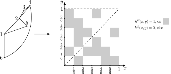
Figure 1: An example of a graph $G$ and its graphon representation $h^{G}$.

The space of graphons $W$ is endowed with the cut distance

$$d_{\square}(h_{1},h_{2}):=\sup_{S,T\subset[0,1]}\left|\int_{S\times T}\mathrm{d}x\,\mathrm{d}y\,[h_{1}(x,y)-h_{2}(x,y)]\right|,\qquad h_{1},h_{2}\in W.$$ (2.12)

On $W$ there is a natural equivalence relation $\equiv$. Let $\Sigma$ be the space of measure-preserving bijections $\sigma\colon\,[0,1]\to[0,1]$. Then $h_{1}(x,y)\equiv h_{2}(x,y)$ if $h_{1}(x,y)=h_{2}(\sigma x,\sigma y)$ for some $\sigma\in\Sigma$. This equivalence relation yields the quotient space $(\tilde{W},\delta_{\square})$, where $\delta_{\square}$ is the metric defined by

$$\delta_{\square}(\tilde{h}_{1},\tilde{h}_{2}):=\inf_{\sigma_{1},\sigma_{2}}d_{\square}(h_{1}^{\sigma_{1}},h_{2}^{\sigma_{2}}),\qquad\tilde{h}_{1},\tilde{h}_{2}\in\tilde{W}.$$ (2.13)

To avoid cumbersome notation, throughout the sequel we suppress the $n$-dependence. Thus, by $G$ we denote any simple graph on $n$ vertices, by $h^{G}$ its image in the graphon space $W$, and by $\tilde{h}^{G}$ its image in the quotient space $\tilde{W}$. Let $F$ and $G$ denote two simple graphs with vertex sets $V(F)$ and $V(G)$, respectively, and let $\text{hom}(F,G)$ be the number of homomorphisms from $F$ to $G$. The homomorphism density is defined as

$$t(F,G):=\frac{1}{|V(G)|^{|V(F)|}}\,\text{hom}(F,G).$$ (2.14)

Two graphs are said to be similar when they have similar homomorphism densities.

Definition 2.3.

A sequence of labelled simple graphs $(G_{n})_{n\in\mathbb{N}}$ is left-convergent when $(t(F,G_{n}))_{n\in\mathbb{N}}$ converges for any simple graph $F$. ∎

Consider a simple graph $F$ on $k$ vertices with edge set $E(F)$, and let $h\in W$. Similarly as above, define the density

$$t(F,h):=\int_{[0,1]^{k}}\mathrm{d}x_{1}\cdots\mathrm{d}x_{k}\prod_{(i,j)\in E(F)}h(x_{i},x_{j}).$$ (2.15)

If $h^{G}$ is the image of a graph $G$ in the space $W$, then

$$t(F,h^{G})=\int_{[0,1]^{k}}\mathrm{d}x_{1}\cdots\mathrm{d}x_{k}\prod_{(i,j)\in E(F)}h^{G}(x_{i},x_{j})=\frac{1}{|V(G)|^{|V(F)|}}\,\text{hom}(F,G)=t(F,G).$$ (2.16)

Hence a sequence of graphs $(G_{n})_{n\in\mathbb{N}}$ is left-convergent to $h\in W$ when

$$\lim_{n\to\infty}t(F,G_{n})=t(F,h).$$ (2.17)

We conclude this section with three basic facts that will be needed later on. The first gives the relation between left-convergence of sequences of graphs and convergence in the quotient space $(\tilde{W},\delta_{\square})$, the second is a compactness property, while the third shows that the homomorphism density is Lipschitz continuous with respect to the $\delta_{\square}$-metric.

Proposition 2.4 (Borgs et al. [4]).

For a sequence of labelled simple graphs $(G_{n})_{n\in\mathbb{N}}$ the following properties are equivalent:
(i) $(G_{n})_{n\in\mathbb{N}}$ is left-convergent.
(ii) $(\tilde{h}^{G_{n}})_{n\in\mathbb{N}}$ is a Cauchy sequence in the metric $\delta_{\square}$.
(iii) $(t(F,h^{G_{n}}))_{n\in\mathbb{N}}$ converges for all finite simple graphs $F$.
(iv) There exists an $h\in W$ such that $\lim_{n\to\infty}t(F,h^{G_{n}})=t(F,h)$ for all finite simple graphs $F$.

Proposition 2.5 (Lovász and Szegedy [20]).

$(\tilde{W},\delta_{\square})$ is compact.

Proposition 2.6 (Borgs et al. [4]).

Let $G_{1},G_{2}$ be two labelled simple graphs, and let $F$ be a simple graph. Then

$$|t(F,G_{1})-t(F,G_{2})|\leq 4|E(F)|\delta_{\square}(G_{1},G_{2}).$$ (2.18)

For a more detailed description of the structure of the space $(\tilde{W},\delta_{\square})$ we refer the reader to Borgs et al. [4, 5] and Diao et at. [12].

2.3 Large deviation principle for the Erdős-Rényi random graph

In this section we recall a few key facts from the literature about rare events in Erdős-Rényi random graphs, formulated in terms of a large deviation principle. Importantly, the scale that is used is $n^{2}$, the order of the number of edges in the graph.

We start by introducing the large deviation rate function. For $p\in(0,1)$ and $u\in[0,1]$, let

$$I_{p}(u) :=\frac{1}{2}u\log\left(\frac{u}{p}\right)+\frac{1}{2}(1-u)\log\left(\frac{1-u}{1-p}\right),$$ (2.19)

$$I(u) :=\frac{1}{2}u\log u+\frac{1}{2}(1-u)\log(1-u)=I_{\tfrac{1}{2}}(u)-\tfrac{1}{2}\log 2,$$

with the convention that $0\log 0=0$. For $h\in W$ we write, with a mild abuse of notation,

$$I_{p}(h):=\int_{[0,1]^{2}}\mathrm{d}x\,\mathrm{d}y\,\,I_{p}(h(x,y)),\qquad I(h):=\int_{[0,1]^{2}}\mathrm{d}x\,\mathrm{d}y\,\,I(h(x,y)).$$ (2.20)

On the quotient space $(\tilde{W},\delta_{\square})$ we define $I_{p}(\tilde{h})=I_{p}(h)$, where $h$ is any element of the equivalence class $\tilde{h}$.

Proposition 2.7 (Chatterjee and Varadhan [11]).

The function $I_{p}$ is well-defined on $\tilde{W}$ and is lower semi-continuous under the $\delta_{\square}$-metric.

Consider the set $\mathcal{G}_{n}$ of all graphs on $n$ vertices and the Erdős-Rényi probability distribution $\mathbb{P}_{n,p}$ on $\mathcal{G}_{n}$. Through the mappings $G\to h^{G}\to\tilde{h}^{G}$ we obtain a probability distribution on $W$ (with a slight abuse of notation again denoted by $\mathbb{P}_{n,p}$), and a probability distribution $\tilde{\mathbb{P}}_{n,p}$ on $\tilde{W}$.

Theorem 2.8 (Chatterjee and Varadhan [11]).

For every $p\in(0,1)$, the sequence of probability distributions $(\tilde{\mathbb{P}}_{n,p})_{n\in\mathbb{N}}$ satisfies the large deviation principle on $(\tilde{W},\delta_{\square})$ with rate function $I_{p}$ defined by (2.20), i.e.,

$$\limsup_{n\to\infty}\frac{1}{n^{2}}\,\log\tilde{\mathbb{P}}_{n,p}(\tilde{C}) \leq-\inf_{\tilde{h}\in\tilde{W}}I_{p}(\tilde{h})\qquad\forall\,\tilde{C}\subset\tilde{W}\mbox{ closed},$$ (2.21)

$$\liminf_{n\to\infty}\ \frac{1}{n^{2}}\,\log\tilde{\mathbb{P}}_{n,p}(\tilde{O}) \geq-\inf_{\tilde{h}\in\tilde{O}}I_{p}(\tilde{h})\qquad\,\,\,\forall\,\tilde{O}\subset\tilde{W}\mbox{ open}.$$

Using the large deviation principle we can find asymptotic expressions for the number of simple graphs on $n$ vertices with a given property. In what follows a property of a graph is defined through an operator $T\colon\,W\to\mathbb{R}^{m}$ for some $m\in\mathbb{N}$. We assume that the operator $T$ is continuous with respect to the $\delta_{\square}$-metric, and for some $\vec{T}^{*}\in\mathbb{R}^{m}$ we consider the sets

$$\tilde{W}^{*}:=\big{\{}\tilde{h}\in\tilde{W}\colon\,T(\tilde{h})=\vec{T}^{*}\big{\}},\qquad\tilde{W}^{*}_{n}:=\big{\{}\tilde{h}\in\tilde{W}^{*}\colon\,\tilde{h}=\tilde{h}^{G}\text{ for some }G\text{ on }n\text{ vertices}\big{\}}.$$ (2.22)

By the continuity of the operator $T$, the set $\tilde{W}^{*}$ is closed. Therefore, using Theorem 2.8, we obtain the following asymptotics for the cardinality of $\tilde{W}^{*}_{n}$.

Corollary 2.9 (Chatterjee [6]).

For any measurable set $\tilde{W}^{*}\subset\tilde{W}$, with $\tilde{W}^{*}_{n}$ as defined in (2.22),

$$-\inf_{\tilde{h}\in{\rm int}(\tilde{W}^{*})}I(\tilde{h})\leq\liminf_{n\to\infty}\frac{\log|\tilde{W}^{*}_{n}|}{n^{2}}\leq\limsup_{n\to\infty}\frac{\log|\tilde{W}^{*}_{n}|}{n^{2}}\leq-\inf_{\tilde{h}\in\tilde{W}^{*}}I(\tilde{h}),$$ (2.23)

where ${\rm int}(\tilde{W}^{*})$ is the interior of $\tilde{W}^{*}$.

3 Variational characterisation of ensemble equivalence

In this section we present a number of preparatory results we will need in Section 4 to state our theorem on the equivalence between $\mathrm{P}_{\mathrm{mic}}$ and $\mathrm{P}_{\mathrm{can}}$. Our main result is Theorem 3.4 below, which gives us a variational characterisation of ensemble equivalence. In Section 3.1 we introduce our constraints on the subgraph counts. In Section 3.2 we rephrase the canonical ensemble in terms of graphons. In Section 3.3 we state and prove Theorem 3.4.

3.1 Subgraph counts

First we introduce the concept of subgraph counts, and point out how the corresponding canonical distribution is defined. Label the simple graphs in any order, e.g., $F_{1}$ is an edge, $F_{2}$ is a wedge, $F_{3}$ is triangle, etc. Let $C_{k}(G)$ denote the number of subgraphs $F_{k}$ in $G$. In the dense regime, $C_{k}(G)$ grows like $n^{V_{k}}$, where $V_{k}=|V(F_{k})|$ is the number of vertices in $F_{k}$. For $m\in\mathbb{N}$, consider the following scaled vector-valued function on $\mathcal{G}_{n}$:

$$\vec{C}(G):=\left(\frac{p(F_{k})C_{k}(G)}{n^{V_{k}-2}}\right)_{k=1}^{m}=n^{2}\left(\frac{p(F_{k})C_{k}(G)}{n^{V_{k}}}\right)_{k=1}^{m}.$$ (3.1)

The term $p(F_{k})$ counts the edge-preserving permutations of the vertices of $F_{k}$, i.e., $p(F_{1})=2$ for an edge, $p(F_{2})=2$ for a wedge, $p(F_{3})=6$ for a triangle, etc. The term $C_{k}(G)/n^{V_{k}}$ represents a subgraph density in the graph $G$. The additional $n^{2}$ guarantees that the full vector scales like $n^{2}$, the scaling of the large deviation principle in Theorem 2.8. For a simple graph $F_{k}$ we define the homomorphism density as

$$t(F_{k},G):=\frac{\text{hom}(F_{k},G)}{n^{V_{k}}}=\frac{p(F_{k})C_{k}(G)}{n^{V_{k}}},$$ (3.2)

which does not distinguish between permutations of the vertices. Hence the Hamiltonian becomes

$$H(\vec{\theta},\vec{T}(G))=n^{2}\sum_{k=1}^{m}\theta_{k}\,t(F_{k},G)=n^{2}(\vec{\theta}\cdot\vec{T}(G)),\qquad G\in\mathcal{G}_{n},$$ (3.3)

where

$$\vec{T}(G):=\left(t(F_{k},G)\right)_{k=1}^{m}.$$ (3.4)

The canonical ensemble with parameter $\vec{\theta}$ thus takes the form

$$\mathrm{P}_{\mathrm{can}}(G\mid\vec{\theta}\,):=\mathrm{e}^{n^{2}\big{[}\vec{\theta}\cdot\vec{T}(G)-\psi_{n}(\vec{\theta}\,)\big{]}},\qquad G\in\mathcal{G}_{n},$$ (3.5)

where $\psi_{n}$ replaces the partition function:

$$\psi_{n}(\vec{\theta}):=\frac{1}{n^{2}}\log\sum_{G\in\mathcal{G}_{n}}\mathrm{e}^{n^{2}(\vec{\theta}\hskip 2.0pt\cdot\hskip 2.0pt\vec{T}(G))}.$$ (3.6)

In the sequel we take $\vec{\theta}$ equal to a specific value $\vec{\theta}^{*}$, so as to meet the soft constraint, i.e.,

$$\langle\vec{T}\rangle=\sum_{G\in\mathcal{G}_{n}}\vec{T}(G)\,\mathrm{P}_{\mathrm{can}}(G)=\vec{T}^{*}.$$ (3.7)

The canonical probability then becomes

$$\mathrm{P}_{\mathrm{can}}(G)=\mathrm{P}_{\mathrm{can}}(G\mid\vec{\theta^{*}})$$ (3.8)

In Section 5.1 we will discuss how to find $\vec{\theta}^{*}$.

Remark 3.1.

(i) The constraint $\vec{T}^{*}$ and the Lagrange multiplier $\vec{\theta}^{*}$ in general depend on $n$, i.e., $\vec{T}^{*}=\vec{T}^{*}_{n}$ and $\vec{\theta}^{*}=\vec{\theta}^{*}_{n}$ (recall Remark 2.2). We consider constraints that converge when we pass to the limit $n\to\infty$, i.e.,

$$\lim_{n\to\infty}\vec{T}^{*}_{n}=\vec{T}^{*}_{\infty}.$$ (3.9)

Consequently, we expect that

$$\lim_{n\to\infty}\vec{\theta}^{*}_{n}=\vec{\theta}^{*}_{\infty}.$$ (3.10)

Throughout the sequel we assume that (3.10) holds. If convergence fails, then we may still consider subsequential convergence. The subtleties concerning (3.10) are discussed in Appendix A.
(ii) In what follows, we suppress the dependence on $n$ and write $\vec{T}^{*},\vec{\theta}^{*}$ instead of $\vec{T}^{*}_{n},\vec{\theta}^{*}_{n}$, but we keep the notation $\vec{T}^{*}_{\infty},\vec{\theta}^{*}_{\infty}$ for the limit. In addition, throughout the sequel we write $\vec{\theta},\vec{\theta}_{\infty}$ instead of $\vec{\theta}^{*},\vec{\theta}_{\infty}^{*}$ when we view these as parameters that do not depend on $n$. This distinction is crucial when we take the limit $n\to\infty$. ∎

3.2 From graphs to graphons

In (2.16) we saw that if we map a finite simple graph $G$ to its graphon $h^{G}$, then for each finite simple graph $F$ the homomorphism densities $t(F,G)$ and $t(F,h^{G})$ are identical. If $(G_{n})_{n\in\mathbb{N}}$ is left-convergent, then

$$\lim_{n\to\infty}\vec{T}(G_{n})=\left(t(F_{k},h)\right)_{k=1}^{m}$$ (3.11)

for some $h\in W$, as an immediate consequence of Theorem 2.4. We further see that the expression in (3.3) can be written in terms of graphons as

$$H(\vec{\theta},\vec{T}(G))=n^{2}\sum_{k=1}^{m}\theta_{k}\,t(F_{k},h^{G}).$$ (3.12)

With this scaling the hard constraint is denoted by $\vec{T}^{*}$, has the interpretation of the density of an observable quantity in $G$, and defines a subspace of the quotient space $\tilde{W}$, which we denote by $\tilde{W}^{*}$, and which consists of all graphons that meet the hard constraint, i.e.,

$$\tilde{W}^{*}:=\{\tilde{h}\in\tilde{W}\colon\,\vec{T}(h)=\vec{T}^{*}\}.$$ (3.13)

The soft constraint in the canonical ensemble becomes $\langle\vec{T}\rangle=\vec{T}^{*}$ (recall (2.5)).

3.3 Variational formula for specific relative entropy

In what follows, the limit as $n\to\infty$ of the partition function $\psi_{n}(\vec{\theta})$ defined in (3.6) plays an important role. This limit has a variational representation that will be key to our analysis.

Theorem 3.2 (Chatterjee and Diaconis [9]).

Let $\vec{T}\colon\,\tilde{W}\rightarrow\mathbb{R}^{m}$be the operator defined in (3.4). For any $\vec{\theta}\in\mathbb{R}^{m}$ (not depending on $n$),

$$\lim_{n\rightarrow\infty}\psi_{n}(\vec{\theta})=\sup_{\tilde{h}\in\tilde{W}}\left(\vec{\theta}\cdot\vec{T}(\tilde{h})-I(\tilde{h})\right)$$ (3.14)

with $I$ and $\psi_{n}$ as defined in (2.20) and (3.6).

Theorem 3.3 (Chatterjee and Diaconis [9]).

Let $F_{1},\ldots,F_{m}$ be subgraphs as defined in Section 3.1. Suppose that $\theta_{2},\ldots,\theta_{m}\geq 0$. Then

$$\lim_{n\rightarrow\infty}\psi_{n}(\vec{\theta})=\sup_{0\leq u\leq 1}\left(\sum_{i=1}^{m}\theta_{i}\,u^{E(F_{k})}-I(u)\right),$$ (3.15)

where $E(F_{k})$ denotes the number of edges in the subgraph $F_{k}$.

The key result in this section is the following variational formula for $s_{\infty}$ defined in Definition 2.1. Recall that for $n\in\mathbb{N}$ we write $\vec{\theta}^{*}$ for $\vec{\theta}^{*}_{n}$.

Theorem 3.4.

Consider the microcanonical ensemble defined in (2.2) with constraint $\vec{T}=\vec{T}^{*}$ defined in (3.4), and the canonical ensemble defined in (3.5)–(3.6) with parameter $\vec{\theta}=\vec{\theta}^{*}$ such that, for every $n\in\mathbb{N}$, (3.7), (3.9) and (3.10) hold. Then

$$s_{\infty}=\lim_{n\to\infty}\frac{1}{n^{2}}\,S_{n}(\mathrm{P}_{\mathrm{mic}}\mid\mathrm{P}_{\mathrm{can}})=\sup_{\tilde{h}\in\tilde{W}}\big{[}\vec{\theta}^{*}_{\infty}\cdot\vec{T}(\tilde{h})-I(\tilde{h})\big{]}-\sup_{\tilde{h}\in\tilde{W}^{*}}\big{[}\vec{\theta}^{*}_{\infty}\cdot\vec{T}(\tilde{h})-I(\tilde{h})\big{]},$$ (3.16)

where $I$ is defined in (2.19) and $\tilde{W}^{*}=\{\tilde{h}\in\tilde{W}\colon\,\vec{T}(\tilde{h})=\vec{T}^{*}_{\infty}\}$.

Proof.

From (2.10) we have

$$s_{\infty}=\lim_{n\to\infty}\frac{1}{n^{2}}\big{[}\log\,\mathrm{P}_{\mathrm{mic}}(G^{*})-\log\,\mathrm{P}_{\mathrm{can}}(G^{*})\big{]},$$ (3.17)

where $G^{*}$ is any graph in $\mathcal{G}_{n}$ such that $\vec{T}(G^{*})=\vec{T}^{*}$. For the microcanonical ensemble we have

$$\log\mathrm{P}_{\mathrm{mic}}(G^{*})=-\log\Omega_{\vec{T}^{*}}=-\log\mathbb{P}_{\frac{1}{2},n}\left(\{G\in\mathcal{G}_{n}\colon\,\vec{T}(G)=\vec{T}^{*}\}\right)-{n\choose 2}\log 2,$$ (3.18)

where

$$\Omega_{\vec{T}^{*}}=|\{G\in\mathcal{G}_{n}\colon\,\vec{T}(G)=\vec{T}^{*}\}|>0.$$ (3.19)

Define the operator $\vec{T}\colon\,W\to\mathbb{R}^{m}$, $h\mapsto(t(F_{k},h))_{k=1}^{m}$. This operator can be extended to an operator (with a slight abuse of notation again denoted by $\vec{T}$) on the quotient space $(\tilde{W},\delta_{\square})$ by defining $\vec{T}(\tilde{h})=\vec{T}(h)$ with $h\in\tilde{h}$. Define the following sets

$$\tilde{W}^{*}:=\big{\{}\tilde{h}\in\tilde{W}\colon\,T(\tilde{h})=\vec{T}^{*}_{\infty}\big{\}},\qquad\tilde{W}^{*}_{n}:=\big{\{}\tilde{h}\in\tilde{W}^{*}\colon\,\tilde{h}=\tilde{h}^{G}\text{ for some }G\in\mathcal{G}_{n}\big{\}}.$$ (3.20)

From the continuity of the operator $\vec{T}$ on $\tilde{W}$, we see that $\tilde{W}^{*}$ is a compact subspace of $\tilde{W}$, and hence is also closed. From Theorem 2.6 we have that $\vec{T}$ is a Lipschitz continuous operator on the space $(\tilde{W},\delta_{\square})$. Since $\tilde{W}$ is a compact space, we have that

$$\lim_{n\to\infty}\frac{1}{n^{2}}\,\log\mathbb{P}_{\frac{1}{2},n}\left(\{G\in\mathcal{G}_{n}\colon\,\vec{T}(G)=\vec{T}^{*}\}\right)=-\inf_{\tilde{h}\in\tilde{W}^{*}}I_{\frac{1}{2}}(\tilde{h})=-\inf_{\tilde{h}\in\tilde{W}^{*}}I(\tilde{h})-\tfrac{1}{2}\log 2.$$ (3.21)

The large deviation principle applied to (3.18) yields

$$\lim_{n\to\infty}\frac{1}{n^{2}}\,\log\mathrm{P}_{\mathrm{mic}}(G^{*})=\inf_{\tilde{h}\in\tilde{W}^{*}}I(\tilde{h}).$$ (3.22)

Consider the canonical ensemble and a graph $G_{n}^{*}$ on $n$ vertices such that $\vec{T}(G_{n}^{*})=\vec{T}^{*}$. By Definition 2.3, Proposition 2.4, and (3.9) we may suppose that $(G_{n}^{*})_{n\in\mathbb{N}}$ is left-convergent and converges to the graphon $h^{*}$. Since $\vec{T}$ is continuous, we have that $\vec{T}(G_{n}^{*})$ converges to $\vec{T}(h^{*})=\vec{T}^{*}_{\infty}$. From (3.5) we have that

$$\lim_{n\to\infty}\frac{1}{n^{2}}\,\log\mathrm{P}_{\mathrm{can}}(G_{n}^{*})=\vec{\theta}^{*}_{\infty}\cdot\vec{T}^{*}_{\infty}-\psi_{\infty}(\vec{\theta}^{*}_{\infty}).$$ (3.23)

By Theorem 3.2,

$$\psi_{\infty}(\vec{\theta}^{*}_{\infty})=\sup_{\tilde{h}\in\tilde{W}}\big{[}\vec{\theta}^{*}_{\infty}\cdot\vec{T}(\tilde{h})-I(\tilde{h})\big{]}.$$ (3.24)

There is an additional subtlety in proving (3.24) in our setup because $\vec{\theta}^{*}$ depends on $n$. This dependence is treated in Appendix A. Combining (3.22) and (3.24), we get

$$s_{\infty}=\lim_{n\to\infty}\frac{1}{n^{2}}\,S_{n}(\mathrm{P}_{\mathrm{mic}}\mid\mathrm{P}_{\mathrm{can}})=\inf_{\tilde{h}\in\tilde{W}^{*}}I(\tilde{h})-\vec{\theta}^{*}_{\infty}\cdot\vec{T}^{*}_{\infty}+\sup_{\tilde{h}\in\tilde{W}}\big{[}\vec{\theta}^{*}_{\infty}\cdot\vec{T}(\tilde{h})-I(\tilde{h})\big{]}.$$ (3.25)

By definition all elements $\tilde{h}\in\tilde{W}^{*}$ satisfy $\vec{T}(\tilde{h})=\vec{T}^{*}_{\infty}$. Hence the expression in the right-hand side of (3.25) can be written as

$$\sup_{\tilde{h}\in\tilde{W}}\big{[}\vec{\theta}^{*}_{\infty}\cdot\vec{T}(\tilde{h})-I(\tilde{h})\big{]}-\sup_{\tilde{h}\in\tilde{W}^{*}}\big{[}\vec{\theta}^{*}_{\infty}\cdot\vec{T}(\tilde{h})-I(\tilde{h})\big{]},$$ (3.26)

which settles the claim. ∎

Remark 3.5.

Theorem 3.4 and the compactness of $\tilde{W}^{*}$ give us a variational characterisation of ensemble equivalence: $s_{\infty}=0$ if and only if at least one of the maximisers of $\vec{\theta}^{*}_{\infty}\cdot\vec{T}(\tilde{h})-I(\tilde{h})$ in $\tilde{W}$ also lies in $\tilde{W}^{*}\subset\tilde{W}$. Equivalently, $s_{\infty}=0$ when at least one the maximisers of $\vec{\theta}^{*}_{\infty}\cdot\vec{T}(\tilde{h})-I(\tilde{h})$ satisfies the hard constraint. ∎

4 Main theorem

The variational formula for the relative entropy $s_{\infty}$ in Theorem 3.4 allows us to identify examples where ensemble equivalence holds ($s_{\infty}=0$) or is broken ($s_{\infty}>0$). We already know that if the constraint is on the edge density alone, i.e., $T(G)=t(F_{1},G)=T^{*}$, then $s_{\infty}=0$ (see Garlaschelli et al. [15]). In what follows we will look at three models:

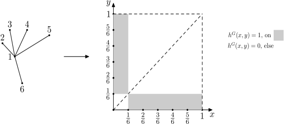
Figure 2: A 5-star graph and its graphon representation.

• The constraint is on the triangle density, i.e., $\vec{T_{2}}(G)=t(F_{3},G)=T_{2}^{*}$ with $F_{3}$ the triangle. This will be referred to as the Triangle Model.

• The constraint is on the edge density and triangle density, i.e., $\vec{T}(G)=(t(F_{1},G),$ $t(F_{3},G))=(T_{1}^{*},T_{2}^{*})$ with $F_{1}$ the edge and $F_{3}$ the triangle. This will be referred to as the Edge-Triangle Model.

• The constraint is on the $j$-star density, i.e., $\vec{T}(G)=t(T[j],G)=T[j]^{*}$ with $T[j]$ the $j$-star graph, consisting of 1 root vertex and $j\in\mathbb{N}\setminus\{1\}$ vertices connected to the root but not connected to each other (see Fig. 2). This will be referred to as the Star Model.

For a graphon $h\in W$ (recall (2.15)), the edge density and the triangle density equal

$$T_{1}(h)=\int_{[0,1]^{2}}\mathrm{d}x_{1}\mathrm{d}x_{2}\,h(x_{1},x_{2}),\quad T_{2}(h)=\int_{[0,1]^{3}}\mathrm{d}x_{1}\mathrm{d}x_{2}\mathrm{d}x_{3}\,h(x_{1},x_{2})h(x_{2},x_{3})h(x_{3},x_{1}),$$ (4.1)

while the $j$-star density equals

$$T[j](h)=\int_{[0,1]}\mathrm{d}x\int_{[0,1]^{j}}\mathrm{d}x_{1}\mathrm{d}x_{2}\cdots\mathrm{d}x_{j}\,\prod_{i=1}^{j}h(x,x_{i}).$$ (4.2)

Theorem 4.1.

For the above three types of constraint:

• • If $T_{2}^{*}\geq\tfrac{1}{8}$ , then $s_{\infty}=0$.

  • If $T_{2}^{*}=0$, then $s_{\infty}=0$.

• • If $T_{2}^{*}=T_{1}^{*{3}}$, then $s_{\infty}=0$.

  • If $T_{2}^{*}\neq T_{1}^{*{3}}$ and $T_{2}^{*}\geq\tfrac{1}{8}$, then $s_{\infty}>0$.

  • If $T_{2}^{*}\neq T_{1}^{*{3}}$, $0<T_{1}^{*}\leq\tfrac{1}{2}$ and $0<T_{2}^{*}<\frac{1}{8}$, then $s_{\infty}>0$.

  • If $T_{1}^{*}=\tfrac{1}{2}+\epsilon$ with $\epsilon\in\left(\frac{\ell-2}{2\ell},\frac{\ell-1}{2\ell+2}\right)$, $\ell\in\mathbb{N}\setminus\{1\}$, and $T_{2}^{*}$ is such that $(T_{1}^{*},T_{2}^{*})$ lies on the scallopy curve in Fig. 3, then $s_{\infty}>0$.

  • If $0<T_{1}^{*}\leq\frac{1}{2}$ and $T_{2}^{*}=0$, then $s_{\infty}=0$.

• For every $j\in\mathbb{N}\setminus\{1\}$, if $T[j]^{*}\geq 0$, then $s_{\infty}=0$.

Here, $T_{1}^{*},T_{2}^{*},T[j]^{*}$ are in fact the limits $T_{1,\infty}^{*},T_{2,\infty}^{*},T[j]^{*}_{\infty}$ in (3.9), but in order to keep the notation light we now also suppress the index $\infty$.

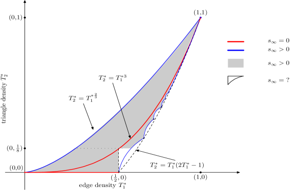
Figure 3: The admissible edge-triangle density region is the region on and between the blue curves (cf. Radin and Sadun [24]).

Theorem 4.1, which states our main results on ensemble equivalence and which is proven in Sections 5–6, is illustrated in Fig. 3. The region on and between the blue curves corresponds to the set of all realisable graphs: if the pair $(e,t)$ lies in this region, then there exists a graph with edge density $e$ and triangle density $t$. The red curves represent ensemble equivalence, the blue curves and the grey region represent breaking of ensemble equivalence, while in the white region between the red curve and the lower blue curve we do not know what happens. Breaking of ensemble equivalence arises from frustration between the edge and the triangle density.

Each of the cases in Theorem 4.1 corresponds to typical behaviour of graphs drawn from the two ensembles:

• In cases (I)(a) and (II)(a), graphs drawn from both ensembles are asymptotically like Erdős-Rényi random graphs with parameter $p=T_{2}^{*1/3}$.

• In cases (I)(b) and (II)(e), almost all graphs drawn from both ensembles are asymptotically like bipartite graphs.

• In cases (II)(b), (II)(c) and (II)(d), we do not know what graphs drawn from the canonical ensemble look like. Graphs drawn from the microcanonical ensemble do not look like Erdős-Rényi random graphs. The structure of graphs drawn from the microcanonical ensemble when the constraint is as in (II)(d) has been determined in Pirkhurko and Razborov [26] and Radin and Sadun [24]. The vertex set of a graph drawn from the microcanonical ensemble can be partitioned into $\ell$ subsets: the first $\ell-1$ have size $\lfloor cn\rfloor$ and the last has size between $\lfloor cn\rfloor$ and $2\lfloor cn\rfloor$, where $c$ is a known constant depending on $\ell$. The graph has the form of a complete $\ell-$partite graph on these pieces, plus some additional edges in the last piece that create no additional triangles.

• In case (III), graphs drawn from both ensembles are asymptotically like Erdős-Rényi random graphs with parameter $p=T[j]^{*1/j}$.

Remark 4.2.

Similar results hold for the Edge-Wedge-Triangle Model and the Edge-Star Model. ∎

Here are three open questions:

• Identify in which cases (3.9) implies (3.10).

• Is $s_{\infty}=0$ as soon as the constraint involves a single subgraph count only?

• What happens for subgraphs other than edges, wedges, triangles and stars? Is again $s_{\infty}>0$ under appropriate frustration?

5 Choice of the tuning parameter

The tuning parameter is to be chosen so as to satisfy the soft constraint (3.7), a procedure that in equilibrium statistical physics is referred to as the averaging principle. Depending on the choice of constraint, finding $\vec{\theta}^{*}$ may not be easy, neither analytically nor numerically. In Section 5.1 we investigate how $\vec{\theta}^{*}$ behaves as we vary $\vec{T}^{*}$ for fixed $n$. We focus on the Edge-Triangle Model (a slight adjustment yields the same results for the Triangle Model). In Section 5.2 we investigate how averages under the canonical ensemble, like (3.7), behave when $n\to\infty$. Here we can treat general constraints defined in (3.4).

For the behaviour of our constrained models, the sign of the coordinates of the tuning parameter $\vec{\theta}^{*}$ is of pivotal importance, both for a fixed $n\in\mathbb{N}$ and asymptotically (see Bhamidi et al. [3], Chatterjee and Diaconis [9], Radin and Yin [25], and references therein). We must therefore carefully keep track of this sign. The key results in this direction are Lemmas 5.1 and 5.2 below.

5.1 Tuning parameter for fixed $n$

Lemma 5.1.

Consider the Triangle Model with the constraint given by the triangle density $T_{2}^{*}$. For every $n$, $\theta^{*}\geq 0$ if and only if $T_{2}^{*}\geq\tfrac{1}{8}$.

Proof.

The proof is similar to that of Lemma 5.2 below. ∎

Lemma 5.2.

Consider the Edge-Triangle Model. For every $n$, $\theta_{2}^{*}\geq 0$ if and only if $T_{2}^{*}\geq\frac{1}{8}$, irrespective of $T_{1}^{*}$. Furthermore, $\theta_{1}^{*}\geq 0$ if and only if $T_{1}^{*}\geq\frac{1}{2}$.

Proof.

Define, for $\theta_{1},\theta_{2}\in\mathbb{R}$, the function

$$g(\theta_{1},\theta_{2}):=\sum_{G\in\mathcal{G}_{n}}\exp\left[n^{2}\left(\theta_{1}(T_{1}(G)-\tfrac{1}{2})+\theta_{2}(T_{2}(G)-\tfrac{1}{8})\right)\right].$$ (5.1)

We first prove that $g$ attains a unique global minimum at $(\theta_{1},\theta_{2})=(0,0)$. Consider the canonical ensemble $\mathrm{P}_{\mathrm{can}}$ as defined in (3.5) and (3.8), with $\vec{T}$ as defined above, and the probability distribution $\mathrm{P}_{\text{hom}}$ on $\mathcal{G}_{n}$ that assigns probability $2^{-{n\choose 2}}$ to every graph $G\in\mathcal{G}_{n}$. Since $\mathrm{P}_{\text{hom}}$ is absolutely continuous with respect to $\mathrm{P}_{\mathrm{can}}$, the relative entropy $S_{n}(\mathrm{P}_{\text{hom}}|\mathrm{P}_{\mathrm{can}})$ is well defined:

$$S_{n}(\mathrm{P}_{\text{hom}}\mid\mathrm{P}_{\mathrm{can}})=\sum_{G\in\mathcal{G}_{n}}\mathrm{P}_{\text{hom}}(G)\log\frac{\mathrm{P}_{\text{hom}}(G)}{\mathrm{P}_{\mathrm{can}}(G)}\geq 0.$$ (5.2)

Using the form of the canonical ensemble we get, after some straightforward calculations, that, for all $\theta_{1},\theta_{2}\in\mathbb{R}$,

$$\sum_{G\in\mathcal{G}_{n}}\exp\Big{[}n^{2}\big{(}\theta_{1}T_{1}(G)+\theta_{2}T_{2}(G)\big{)}\Big{]}\geq 2^{{n\choose 2}}\exp\left[n^{2}\big{(}\theta_{1}\tfrac{1}{2}+\theta_{2}\tfrac{1}{8}\big{)}\right],$$ (5.3)

where the term in the right-hand side comes from the relation

$$\sum_{G\in\mathcal{G}_{n}}\frac{1}{2^{{n\choose 2}}}\left(\theta_{1}T_{1}(G)+\theta_{2}T_{2}(G)\right)=\theta_{1}\tfrac{1}{2}+\theta_{2}\tfrac{1}{8}.$$ (5.4)

Observe that the left-hand side represents the average edge and triangle density, multiplied with $\theta_{1},\theta_{2}$, in an Erdős-Rényi random graph with parameters $(n,\frac{1}{2})$. From (5.3) we find that $g(\theta_{1},\theta_{2})\geq 2^{{n\choose 2}}=g(0,0)$ for all $\theta_{1},\theta_{2}\in\mathbb{R}$, and so $g$ attains a global minimum at $(0,0)$. In what follows we show that this global minimum is unique. A straightforward computation shows that $\partial_{\theta_{1}}g(\theta_{1},\theta_{2})=\partial_{\theta_{2}}g(\theta_{1},\theta_{2})=0$ if and only if $\langle T_{1}\rangle=\tfrac{1}{2}$ and $\langle T_{2}\rangle=\tfrac{1}{8}$. Furthermore, the Hessian matrix is a covariance matrix and hence is positive semi-definite. For $\vec{\theta}=(\theta_{1},\theta_{2})=(0,0)$ we know that $\langle T_{1}\rangle=\tfrac{1}{2}$ and $\langle T_{2}\rangle=\tfrac{1}{8}$. Hence, by uniqueness of the multiplier $\vec{\theta}^{*}$ for the constraint $T_{1}^{*}=\tfrac{1}{2}$, $T_{2}^{*}=\tfrac{1}{8}$, we obtain that $g$ has a unique global minimum at $(0,0)$. Moreover, this shows that $g$ has no other stationary points. Consider the parameter $(\theta_{1},\theta_{2})=(\theta_{1}^{*},\theta_{2}^{*})$. We have

$$\partial_{\theta_{2}}g(\theta_{1}^{*},\theta_{2}^{*}) =\left(\langle T_{2}\rangle-\tfrac{1}{8}\right)\text{exp}[-n^{2}(\theta_{1}^{*}\tfrac{1}{2}+\theta_{2}^{*}\tfrac{1}{8})]\sum_{G\in\mathcal{G}_{n}}\exp\left[n^{2}\left(\theta_{1}^{*}T_{1}(G)+\theta_{2}^{*}T_{2}(G)\right)\right]$$ (5.5)

$$=\left(T_{2}^{*}-\tfrac{1}{8}\right)\text{exp}[-n^{2}(\theta_{1}^{*}\tfrac{1}{2}+\theta_{2}^{*}\tfrac{1}{8})]\sum_{G\in\mathcal{G}_{n}}\exp\left[n^{2}\left(\theta_{1}^{*}T_{1}(G)+\theta_{2}^{*}T_{2}(G)\right)\right].$$

If $T_{2}^{*}\geq\tfrac{1}{8}$, then $\partial_{\theta_{2}}g(\theta_{1}^{*},\theta_{2}^{*})\geq 0$. Because $g$ has a unique stationary point at $(0,0)$, which is a global minimum, we get $\theta_{2}^{*}\geq 0$. Similarly, we can show that if $T_{2}^{*}<\tfrac{1}{8}$, then $\theta_{2}^{*}<0$. Suppose that $T_{1}^{*}\geq\tfrac{1}{2}$. For the parameter $(\theta_{1},\theta_{2})=(\theta_{1}^{*},\theta_{2}^{*})$ we have

$$\partial_{\theta_{1}}g(\theta_{1}^{*},\theta_{2}^{*}) =\left(\langle T_{1}\rangle-\tfrac{1}{2}\right)\text{exp}[-n^{2}(\theta_{1}^{*}\tfrac{1}{2}+\theta_{2}^{*}\tfrac{1}{8})]\sum_{G\in\mathcal{G}_{n}}\exp\left[n^{2}\left(\theta_{1}^{*}T_{1}(G)+\theta_{2}^{*}T_{2}(G)\right)\right]$$ (5.6)

$$=\left(T_{1}^{*}-\tfrac{1}{2}\right)\text{exp}[-n^{2}(\theta_{1}^{*}\tfrac{1}{2}+\theta_{2}^{*}\tfrac{1}{8})]\sum_{G\in\mathcal{G}_{n}}\exp\left[n^{2}\left(\theta_{1}^{*}T_{1}(G)+\theta_{2}^{*}T_{2}(G)\right)\right].$$

Arguing in a similar way as before, we conclude that $\theta_{1}^{*}\geq 0$ if and only if $T_{1}^{*}\geq\frac{1}{2}$. ∎

Consider the Edge-Triangle Model and suppose that the constraint $(T_{1}^{*},T_{2}^{*})$ is such that $T_{2}^{*}=T_{1}^{*3}$. Then $\theta_{2}^{*}=0$ and $\theta_{1}^{*}$ matches the constraint on the edge density only. The following lemma shows that in this case the canonical ensemble behaves like the Erdős-Rényi model with parameter $T_{1}^{*}$, a fact that will be needed later to prove equivalence.

Lemma 5.3.

Consider the Edge-Triangle Model with the constraint given by the edge-triangle densities $\vec{T}^{*}=(T_{1}^{*},T_{2}^{*})$ with $T_{2}^{*}=T_{1}^{*3}$. Consider the canonical ensemble as defined in (3.8). Then, for every $n\in\mathbb{N}$,

$$\theta_{1}^{*}=\frac{1}{2}\log\frac{T_{1}^{*}}{1-T_{1}^{*}},\qquad\theta^{*}_{2}=0.$$ (5.7)

Proof.

From the definition of the canonical ensemble we have that, for $G\in\mathcal{G}_{n}$,

$$\mathrm{P}_{\mathrm{can}}(G)=\mathrm{P}_{\mathrm{can}}(G\mid\vec{\theta}^{*})=\mathrm{e}^{n^{2}\left[\theta_{1}^{*}T_{1}(G)+\theta_{2}^{*}T_{2}(G)-\psi_{n}(\vec{\theta}^{*})\right]},$$ (5.8)

where $\psi_{n}(\vec{\theta}^{*})$ is the partition function defined in (3.6). For the specific value $\vec{\theta}=\vec{\theta}^{*}$ we have that (recall (3.7))

$$\langle T_{1}\rangle=T_{1}^{*},\qquad\langle T_{2}\rangle=T_{2}^{*}=T_{1}^{*3}.$$ (5.9)

We claim that the correct parameter is $\vec{\theta}^{*}=(\frac{1}{2}\log\frac{T_{1}^{*}}{1-T_{1}^{*}},0)$. The average fraction of edges is $T_{1}^{*}$ (see Park and Newman [22]). The average number of triangles is

$$\langle T_{2}\rangle =\frac{\sum_{G\in\mathcal{G}_{n}}T_{2}(G)\exp\left[n^{2}\left(\frac{1}{2}\log\frac{T_{1}^{*}}{1-T_{1}^{*}}\,T_{1}(G)\right)\right]}{\sum_{G\in\mathcal{G}_{n}}\exp\left[n^{2}\left(\frac{1}{2}\log\frac{T_{1}^{*}}{1-T_{1}^{*}}\,T_{1}(G)\right)\right]}$$

$$=\frac{\sum_{G\in\mathcal{G}_{n}}T_{2}(G)(T_{1}^{*})^{E(G)}(1-T_{1}^{*})^{{n\choose 2}-E(G)}}{\sum_{G\in\mathcal{G}_{n}}(T_{1}^{*})^{E(G)}(1-T_{1}^{*})^{{n\choose 2}-E(G)}}=T_{1}^{*3},$$

where the last equation comes from the fact we are calculating the average number of triangles in an Erdős-Rényi model with probability $T_{1}^{*}$. Since the multiplier $\vec{\theta}^{*}$ is unique, the proof is complete. ∎

5.2 Tuning parameter for $n\to\infty$

In Lemma 5.4 below we show how averages under the canonical ensemble behave asymptotically when $\vec{\theta}$ does not depend on $n$. In Lemma A.2 we will look at what happens when $\vec{\theta}$ is a one-dimensional multiplier and depends on $n$.

Lemma 5.4.

Suppose that the operator $\vec{T}\colon\,W\to\mathbb{R}^{m}$ is bounded and continuous with respect to the $\delta_{\square}$-norm as defined in (2.13). For $\vec{\theta}\in\mathbb{R}^{m}$ independent of $n$, consider the variational problem

$$\sup_{\tilde{h}\in\tilde{W}}\big{[}\vec{\theta}\cdot\vec{T}(\tilde{h})-I(\tilde{h})\big{]},$$ (5.10)

where $I$ is defined in (2.19). Suppose that the supremum is attained at a unique point, denoted by $\tilde{h}^{*}(\vec{\theta})$. Then

$$\lim_{n\to\infty}\sum_{G\in\mathcal{G}_{n}}T_{k}(G)\,\mathrm{P}_{\mathrm{can}}(G\mid\vec{\theta}\,)=T_{k}\big{(}\tilde{h}^{*}(\vec{\theta})\big{)},\qquad k=1,\ldots,m.$$ (5.11)

Proof.

The average of $T_{k}$ under the canonical probability distribution is equal to

$$\sum_{G\in\mathcal{G}_{n}}T_{k}(G)\mathrm{P}_{\mathrm{can}}(G\mid\vec{\theta})=\sum_{G\in\mathcal{G}_{n}}T_{k}(G)\,\mathrm{e}^{n^{2}\left[\vec{\theta}\cdot\vec{T}(G)-\psi_{n}(\vec{\theta})\right]}=:\mathcal{J}_{n}.$$ (5.12)

Pick $\delta>0$ and consider the $\delta$-ball $B_{\delta}(\tilde{h}^{*})$ around the maximiser $\tilde{h}^{*}$ in the quotient space $(\tilde{W},\delta_{\square})$, i.e.,

$$B_{\delta}(\tilde{h}^{*}):=\big{\{}\tilde{h}\in\tilde{W}\colon\delta_{\square}(\tilde{h},\tilde{h}^{*})<\delta\big{\}}.$$ (5.13)

We denote by $G^{\delta}$ a graph on $n$ vertices whose graphon is a representative element of the class $\tilde{h}^{G}$. With a slight abuse of notation, we denote by $G^{\delta}$ both the graph and the corresponding graphon, and by $\tilde{h}^{G}$ the corresponding equivalence class in the quotient space $(\tilde{W},\delta_{\square})$. Since $(\tilde{W},\delta_{\square})$ is compact space (recall Proposition 2.5), and the graphons associated with finite graphs form a countable family that is dense in $(\tilde{W},\delta_{\square})$ (see Diao et al. [12], Lovász and Szegedy [20]), there exists a sequence $(\tilde{h}^{G_{n}})_{n\in\mathbb{N}}$ such that $\lim_{n\to\infty}\delta_{\square}(\tilde{h}^{G_{n}},\tilde{h}^{*})=0$. For $n$ large enough the neighbourhood $B_{\delta}(\tilde{h}^{*})$ contains elements of the sequence $(\tilde{h}^{G_{n}})_{n\in\mathbb{N}}$ and, due to the Lipschitz property (recall Proposition 2.6), $\delta_{\square}(\tilde{h}^{G_{n}},\tilde{h}^{*})<\delta$ implies $|T_{k}(\tilde{h}^{G_{n}})-T_{k}(\tilde{h}^{*})|<C_{k}\delta$ for some constant $C_{k}>0$ and $k=1,\ldots,m$.

Upper bound for $\mathcal{J}_{n}$.

We decompose the sum over $G\in\mathcal{G}_{n}$ into two parts: the first over $G$ whose graphon lies in $B_{\delta}(\tilde{h}^{*})$, the second over $G$ whose graphon lies in $B_{\delta}(\tilde{h}^{*})^{c}=:\tilde{W}^{\delta,\#}$. We further denote by

$$\mathcal{G}_{n}^{\delta}:=\big{\{}G\in\mathcal{G}_{n}\colon\,|T_{k}(\tilde{h}^{G})-T_{k}(\tilde{h}^{*})|<\delta,\hskip 5.69054ptk=1,\ldots,m\big{\}},$$ (5.14)

the set of all graphs whose subgraph densities $T_{k}(G)$ are $\delta$-close to $T_{k}(\tilde{h}^{*})$. A graph from this set is denoted by $G^{\delta}$. We define the set

$$\mathcal{G}_{n}^{\delta,\#}:=\big{\{}G\in\mathcal{G}_{n}\colon\,\tilde{h}^{G}\in\tilde{W}^{\delta,\#}\big{\}}$$ (5.15)

and, for $k=1,\ldots,m$, obtain the following upper bound:

$$\mathcal{J}_{n} = \sum_{G\in\mathcal{G}_{n}^{\delta}}T_{k}(G)\,\mathrm{e}^{n^{2}\left[\vec{\theta}\cdot\vec{T}(G)-\psi_{n}(\vec{\theta})\right]}+\sum_{G\in\mathcal{G}_{n}^{\delta,\#}}T_{k}(G)\,\mathrm{e}^{n^{2}\left[\vec{\theta}\cdot\vec{T}(G)-\psi_{n}(\vec{\theta})\right]}$$ (5.16)

$$\leq \frac{(T_{k}(G^{\delta})+\delta)\sum\limits_{G\in\mathcal{G}_{n}^{\delta}}\mathrm{e}^{n^{2}\vec{\theta}\cdot\vec{T}(G)}}{\sum\limits_{G\in\mathcal{G}_{n}^{\delta}}\mathrm{e}^{n^{2}\vec{\theta}\cdot\vec{T}(G)}}+\sum_{G\in\mathcal{G}_{n}^{\delta,\#}}T_{k}(G)\,\mathrm{e}^{n^{2}\left[\vec{\theta}\cdot\vec{T}(G)-\psi_{n}(\vec{\theta)}\right]}$$

$$= (T_{k}(G^{\delta})+\delta)+\frac{\sum\limits_{G\in\mathcal{G}_{n}^{\delta,\#}}T_{k}(G)\,\mathrm{e}^{n^{2}\vec{\theta}\cdot\vec{T}(G)}}{\sum\limits_{G\in\mathcal{G}_{n}}\mathrm{e}^{n^{2}\vec{\theta}\cdot\vec{T}(G)}}.$$

Next, we further bound the second term in (5.16). By definition, for every $n\in\mathbb{N}$ the range of the operator $\vec{T}$ is a finite set

$$R_{n}:=\big{\{}\vec{g}\in[0,\infty)^{m}\colon\,\vec{T}(G)=\vec{g},\leavevmode\nobreak\ G\in\mathcal{G}_{n}\big{\}}.$$ (5.17)

For the set $R_{n}$ we observe that $|R_{n}|=o(n^{m^{2}})$. In addition, introduce the sets

$$\mathcal{G}_{n}^{\vec{g}} :=\{G\in\mathcal{G}_{n}\colon\,\vec{T}(G)=\vec{g}\},$$ (5.18)

$$R_{n}^{\delta,\#} :=\{\vec{g}\in[0,\infty)^{m}\colon\,\vec{T}(G)=\vec{g},G\in\mathcal{G}_{n}^{\delta,\#}\}\subset R_{n}.$$

The operator $\vec{T}$ is bounded, and so there exists an $M>0$ such that $\|\vec{T}(G)\|\leq M$ for all $G\in\mathcal{G}_{n}$. Hence, the second term in (5.16) can be bounded from above by

$$\frac{\sum_{G\in\mathcal{G}_{n}^{\delta,\#}}T_{k}(G)\,\mathrm{e}^{n^{2}\vec{\theta}\cdot\vec{T}(G)}}{\sum_{G\in\mathcal{G}_{n}}\mathrm{e}^{n^{2}\vec{\theta}\cdot\vec{T}(G)}}\leq\frac{|R_{n}^{\delta,\#}|\,M\,\exp\big{[}n^{2}\sup_{\vec{g}\in R_{n}^{\delta,\#}}(\vec{\theta}\cdot\vec{g}+\frac{1}{n^{2}}\log|\mathcal{G}_{n}^{\vec{g}}|)\big{]}}{\exp\big{[}n^{2}\sup_{\vec{g}\in R_{n}}(\vec{\theta}\cdot\vec{g}+\frac{1}{n^{2}}\log|\mathcal{G}_{n}^{\vec{g}}|)\big{]}}.$$ (5.19)

By the large deviation principle in Theorem 2.8, we have

$$\frac{1}{n^{2}}\,\log|\mathcal{G}_{n}^{\vec{g}}|=\inf_{\tilde{h}\in\tilde{W}^{\vec{g}}}I(h)+o(1),$$ (5.20)

where $\tilde{W}^{g}=\{\tilde{h}\in\tilde{W}\colon\,\vec{T}(\tilde{h})=\vec{g}\}$. As a consequence, (5.19) is majorised by

$$M\,|R_{n}^{*}|\,\mathrm{e}^{o(n^{2})}\exp\left[n^{2}\left(\,\sup_{\vec{g}\in R_{n}^{\delta,\#}}\big{[}\vec{\theta}\cdot\vec{g}-\inf_{\tilde{h}\in\tilde{W}^{\vec{g}}}I(\tilde{h})\big{]}-\sup_{\vec{g}\in R_{n}}\big{[}\vec{\theta}\cdot\vec{g}-\inf_{\tilde{h}\in\tilde{W}^{\vec{g}}}I(\tilde{h})\big{]}\right)\right]$$ (5.21)

$$=M\,|R_{n}^{*}|\,\mathrm{e}^{o(n^{2})}\exp\left[n^{2}\left(\,\sup_{\vec{g}\in R_{n}^{\delta,\#}}\sup_{\tilde{h}\in\tilde{W}^{\vec{g}}}\big{[}\vec{\theta}\cdot\vec{T}(\tilde{h})-I(\tilde{h})\big{]}-\sup_{\vec{g}\in R_{n}}\sup_{\tilde{h}\in\tilde{W}^{\vec{g}}}\big{[}\vec{\theta}\cdot\vec{T}(\tilde{h})-I(\tilde{h})\big{]}\right)\right]$$

$$=M\,|R_{n}^{*}|\,\mathrm{e}^{o(n^{2})}\exp\left[n^{2}\left(\,\sup_{\tilde{h}\in\tilde{W}^{\delta,\#}}\big{[}\vec{\theta}\cdot\vec{T}(\tilde{h})-I(\tilde{h})\big{]}-\sup_{\tilde{h}\in\tilde{W}}\big{[}\vec{\theta}\cdot\vec{T}(\tilde{h})-I(\tilde{h})\big{]}\right)\right].$$

The last equation can be justified as follows. Define the sets

$$\tilde{W}_{n}=\big{\{}\tilde{h}\in\tilde{W}\colon\,\tilde{h}=\tilde{h}^{G}\text{ for some graph }G\in\mathcal{G}_{n}\big{\}},\qquad\tilde{W}^{\delta,\#}_{n}=\tilde{W}^{\delta,\#}\cap\tilde{W}_{n}.$$ (5.22)

Since the graphons associated with finite graphs form a countable set that is dense in $(\tilde{W},\delta_{\square})$, we have that

$$\tilde{W}=\text{cl}\left(\bigcup\limits_{n\in\mathbb{N}}\tilde{W}_{n}\right),\qquad\tilde{W}^{\delta,\#}=\text{cl}\left(\bigcup\limits_{n\in\mathbb{N}}\tilde{W}^{\delta,\#}_{n}\right),$$ (5.23)

where cl denotes closure. Using (5.23), and recalling that $\vec{T}$ is continuous and $I$ is lower-semicontinuous, we get

$$\lim_{n\to\infty}\sup_{\vec{g}\in R_{n}^{\delta,\#}}\sup_{\tilde{h}\in\tilde{W}^{\vec{g}}}\big{[}\vec{\theta}\cdot\vec{T}(\tilde{h})-I(h)\big{]}=\sup_{\tilde{h}\in\tilde{W}^{\delta,\#}}\big{[}\vec{\theta}\cdot\vec{T}(\tilde{h})-I(\tilde{h})\big{]},$$ (5.24)

and a similar result can be established for the second supremum in the exponent in (5.21). The exponent in (5.21) is negative for all $\delta>0$ and is independent of $n$. Moreover, by the left-continuity of the graph sequence $(G_{n}^{\delta})_{n\in\mathbb{N}}$, we have that $\lim_{n\to\infty}T_{k}(G_{n}^{\delta})=T_{k}(\tilde{h}^{*})$ for every $k=1,\ldots,m$ and every $\delta>0$. Combined with the inequality in (5.16), we obtain, for $k=1,\ldots,m$,

$$\lim_{n\to\infty}\sum_{G\in\mathcal{G}_{n}}T_{k}(G)\,\mathrm{e}^{n^{2}\left[\vec{\theta}\cdot\vec{T}(G)-\psi_{n}(\vec{\theta})\right]}\leq T_{k}(\tilde{h}^{*}).$$ (5.25)

Lower bound for $\mathcal{J}_{n}$.

We distinguish two cases: $T_{k}(\tilde{h}^{*})=0$ and $T_{k}(\tilde{h}^{*})>0$. For the first case we trivially get the lower bound

$$\lim_{n\to\infty}\sum_{G\in\mathcal{G}_{n}}T_{k}(G)\,\mathrm{e}^{n^{2}\vec{\theta}\cdot\vec{T}(G)}\geq 0=T_{k}(\tilde{h}^{*}).$$ (5.26)

For the second case we show the equivalent upper bound for the inverse, i.e.,

$$\lim_{n\to\infty}\frac{\sum_{G\in\mathcal{G}_{n}}\mathrm{e}^{n^{2}\vec{\theta}\cdot\vec{T}(G)}}{\sum_{G\in\mathcal{G}_{n}}T_{k}(G)\,\mathrm{e}^{n^{2}\vec{\theta}\cdot\vec{T}(G)}}\leq\frac{1}{T_{k}(\tilde{h}^{*})}.$$ (5.27)

Using the fact that $T_{k}(\tilde{h}^{*})\neq 0$ is bounded, and using a similar reasoning as for the upper bound on $\mathcal{J}_{n}$, the latter is easily verified. ∎

Remark 5.5.

The convergence in (5.11) is not necessarily uniform in $\vec{\theta}$. Our results in Theorem (4.1) (II)(b)-(II)(d) indicate that breaking of ensemble equivalence manifests itself through non uniform convergence in (5.11). In Lemma (A.2) we show that uniform convergence holds when the constraint is on the triangle density only, which explains our result in Theorem (4.1) (I).

Remark 5.6.

The analogue of Lemma 5.4 when the supremum in (5.10) has multiple maximisers in $\tilde{W}$ is considerably more involved. ∎

As observed in Remark 2.2, in general the tuning parameter $\vec{\theta}^{*}$ depends on $n$. We discuss this dependence in Appendix A.

6 Proof of Theorem 4.1

We proceed by computing the relative entropy $s_{\infty}$. In Sections 6.1, 6.3, 6.4, 6.5, 6.6 and 6.8 we treat the limiting regime where all constraints and parameters are the limiting parameters as in (3.9) and (3.10). In Sections 6.2 and 6.7 we write $T^{*}_{\infty,1},T^{*}_{\infty,2},\theta^{*}_{\infty,1}$ for the limiting regime.

6.1 Proof of (I)(a) (Triangle model  $T_{2}^{*}\geq\frac{1}{8})$

Proof.

Theorem 3.4 says that

$$s_{\infty}=\sup_{\tilde{h}\in\tilde{W}}\big{[}\theta^{*}T_{2}(\tilde{h})-I(\tilde{h})\big{]}-\sup_{\tilde{h}\in\tilde{W}^{*}}\big{[}\theta^{*}T_{2}(\tilde{h})-I(\tilde{h})\big{]}.$$ (6.1)

Consider the first term in the right-hand side (6.1). From Lemma 5.1 we know that $\theta^{*}\geq 0$ if and only if $T_{2}^{*}\geq\tfrac{1}{8}$. From Theorem 3.3 it follows that if $\theta^{*}\geq 0$, then

$$\sup_{\tilde{h}\in\tilde{W}}\big{[}\theta^{*}T_{2}(\tilde{h})-I(\tilde{h})\big{]}=\sup_{u\in[0,1]}\big{[}\theta^{*}u^{3}-I(u)\big{]}=\sup_{u\in[0,1]}\ell_{3}(u;\theta^{*}).$$ (6.2)

From Radin and Yin [25, Proposition 3.2] we know that $\ell_{3}(u,\theta^{*})$ attains a unique global maximum. Let $u^{*}(\theta^{*})=\text{arg}\sup_{u\in[0,1]}\ell_{3}(u;\theta^{*})$ be the unique global maximiser. Using Lemma A.2, we obtain that $u^{*}(\theta^{*})={T_{2}^{*}}^{1/3}$, which leads to

$$\sup_{u\in[0,1]}\ell_{3}(u;\theta^{*})=\theta^{*}u^{*}(\theta^{*})^{3}-I\big{(}u^{*}(\theta^{*})\big{)}=\theta^{*}T_{2}^{*}-I\big{(}T_{2}^{*1/3}\big{)}.$$ (6.3)

As to the second term in the right-hand side of (6.1), we use Chatterjee and Varadhan [11, Proposition 4.2], which states that, for $T_{2}^{*}\in(\tfrac{1}{8},1]$,

$$\inf_{\tilde{h}\in\tilde{W}}I(\tilde{h}):=\inf\big{\{}I(\tilde{h})\colon\,\tilde{h}\in\tilde{W},T_{2}(\tilde{h})=T_{2}^{*}\big{\}}=\inf\big{\{}I(\tilde{h})\colon\,\tilde{h}\in\tilde{W},T_{2}(\tilde{h})\geq T_{2}^{*}\big{\}}.$$ (6.4)

Moreover, $I$ is convex at the point $x=T_{2}^{*1/3}$, and hence from Chatterjee and Varadhan [11, Theorem 4.3] we have that $\inf_{\tilde{h}\in\tilde{W}^{*}}I(\tilde{h})=I(T_{2}^{*1/3})$. Combining this with (6.3), we conclude that $s_{\infty}=0$. ∎

6.2 Proof of (I)(b) ($T_{2}^{*}=0$)

Consider the Triangle Model with the constraint given by the triangle density $T^{*}=0$. It was proven by Erdős et al. [13] that almost all triangle-free graph have a bipartite structure. For the case of dense graphs, the condition $T^{*}=0$ means that the number of triangles in the graph is of order $o(n^{2})$. In the proof we will see that the two ensembles are equivalent and that graphs drawn from the two ensembles have a bipartite structure.

Proof.

From the construction of the canonical ensemble $\mathrm{P}_{\mathrm{can}}$ in Section 1.3, we observe that $\mathrm{P}_{\mathrm{can}}(G)=0$ when $T(G)>0$. This is a direct consequence of (2.5). We write

$$\mathcal{G}_{n}^{0}:=\{G\in\mathcal{G}_{n}:T(G)=0\}$$ (6.5)

for the collection of all graphs with triangle density equal to zero. From (2.6) we obtain that $\mathrm{P}_{\mathrm{can}}(G)=0$ if $G\notin\mathcal{G}_{n}^{0}$ and $\mathrm{P}_{\mathrm{can}}(G)=|\mathcal{G}_{n}^{0}|^{-1}$ if $G\in\mathcal{G}_{n}^{0}$. Hence $\mathrm{P}_{\mathrm{can}}(G)=\mathrm{P}_{\mathrm{mic}}(G)$ when the constraint is given by $T^{*}=0$, which yields

$$S_{n}(\mathrm{P}_{\mathrm{mic}}\mid\mathrm{P}_{\mathrm{can}})=0\qquad\forall n\in\mathbb{N}$$ (6.6)

and hence $s_{\infty}=0$. ∎

6.3 Proof of (II)(a) (Edge-Triangle model  $T_{2}^{*}=T_{1}^{*3}$)

For the case $T_{1}^{*}=T_{2}^{*\frac{1}{3}}$ we have shown in Lemma 5.3 that the canonical ensemble essentially behaves like an Erdős-Rényi model with parameter $p=T_{1}^{*}$. Furthermore, the microcanonical ensemble also has an explicit expression, which is found by using the following lemma.

Lemma 6.1.

If $T_{1}^{*}=T_{2}^{*\frac{1}{3}}$, then

$$\inf_{\tilde{h}\in\tilde{W}^{*}}I(\tilde{h})=I\big{(}T_{2}^{*\frac{1}{3}}\big{)}=I\big{(}T_{1}^{*}\big{)}.$$ (6.7)

Proof.

Consider an element $\tilde{h}\in\tilde{W}^{*}$ with $\tilde{W}^{*}:=\{\tilde{h}\in\tilde{W}\colon\,T_{1}(\tilde{h})=T_{1}^{*}=T_{2}^{*\frac{1}{3}},T_{2}(\tilde{h})=T_{2}^{*}\}$. Using the convexity of $I$ on $\tilde{W}$ and Jensen’s inequality, we get

$$I(\tilde{h})=\int_{[0,1]^{2}}\mathrm{d}x\,\mathrm{d}y\,I(h(x,y))\geq I\left(\int_{[0,1]^{2}}\mathrm{d}x\,\mathrm{d}y\,h(x,y)\right)=I\big{(}T_{1}(\tilde{h})\big{)}=I(T_{1}^{*})=I\big{(}T_{2}^{*\frac{1}{3}}\big{)}.$$ (6.8)

Hence $I(\tilde{h})\geq I(T_{2}^{*\frac{1}{3}})$ for every $\tilde{h}\in\tilde{W}^{*}$, which proves the claim. ∎

Proof of (II)(a).

Consider the relative entropy $s_{\infty}$ as defined in (2.9) and (2.10). Using Lemma 5.3, we obtain the expression

$$s_{\infty}=-\frac{1}{2}T_{1}^{*}\log(T_{1}^{*})-\frac{1}{2}(1-T_{1}^{*})\log(1-T_{1}^{*})+\inf_{\tilde{h}\in\tilde{W}^{*}}I(\tilde{h}).$$ (6.9)

From Lemma 6.1 we have that $\inf\limits_{\tilde{h}\in\tilde{W}^{*}}I(\tilde{h})=I(T_{1}^{*})$, which yields $s_{\infty}=0$. ∎

6.4 Proof of (II)(b) ($T_{2}^{*}\neq T_{1}^{*3}$ and $T_{2}^{*}\geq\frac{1}{8}$)

Proof.

From Lemma 5.2 we know that if $T_{1}^{*}\geq\frac{1}{2}$ and $T_{2}^{*}\geq\frac{1}{8}$, then $\theta_{1}^{*}\geq 0$ and $\theta_{2}^{*}\geq 0$ while if $T_{1}^{*}<\frac{1}{2}$ and $T_{2}^{*}\geq\frac{1}{8}$, then $\theta_{1}^{*}<0$ and $\theta_{2}^{*}\geq 0$. An argument similar as above yields

$$\sup\limits_{\tilde{h}\in\tilde{W}}\left[\theta_{1}^{*}T_{1}(\tilde{h})+\theta_{2}^{*}T_{2}(\tilde{h})-I(\tilde{h})\right]=\sup_{u\in[0,1]}\ell_{3}(u;\vec{\theta}^{*}),$$ (6.10)

where for $\theta_{1}^{*}\geq 0$ and $\theta_{2}^{*}\geq 0$ the last supremum has a unique solution (see Radin and Yin [25, Proposition 3.2]), while for $\theta_{1}^{*}<0$ and $\theta_{2}^{*}\geq 0$ it either has a unique solution or two solutions. We treat these two cases separately.

Unique solution.

Because of the uniqueness of the solution, not all realisable hard constraints can be met in the limit (see Lemma 5.4). We observe that, if $T_{2}^{*}\geq\frac{1}{8}$ and $T_{2}^{*}\neq T_{1}^{*{3}}$, in the limit as $n\to\infty$ the canonical ensemble becomes Erdős-Rényi with parameter $p$. This regime is known as the high-temperature regime (see Bhamidi et al. [3] and Chatterjee and Diaconis [9]). In what follows we determine the parameter $p$ of the canonical ensemble in the limit. From Bhamidi et al. [3, Theorem 7] we have that $p=u^{*}(\vec{\theta}^{*})^{\frac{1}{3}}$ with $u^{*}(\vec{\theta}^{*})^{\frac{1}{3}}$ the unique maximiser of (6.10). The expression in (6.10) thus takes the form

$$\sup\limits_{\tilde{h}\in\tilde{W}}\left[\theta_{1}^{*}T_{1}(\tilde{h})+\theta_{2}^{*}T_{2}(\tilde{h})-I(\tilde{h})\right]$$ (6.11)

$$=\sup_{u\in[0,1]}\ell_{3}(u;\vec{\theta}^{*})=\theta_{1}^{*}u^{*}(\vec{\theta}^{*})^{\frac{1}{3}}+\theta_{2}^{*}u^{*}(\vec{\theta}^{*})-I\big{(}u^{*}(\vec{\theta}^{*})^{\frac{1}{3}}\big{)}.$$

Consider the second term in the right-hand side of (3.16). From the definition of $\tilde{W}^{*}$ it is straightforward to see that

$$\sup_{\tilde{h}\in\tilde{W}^{*}}\left[\theta_{1}^{*}T_{1}(\tilde{h})+\theta_{2}^{*}T_{2}(\tilde{h})-I(\tilde{h})\right]=\theta_{1}^{*}T_{1}^{*}+\theta_{2}^{*}T_{2}^{*}-\inf_{\tilde{h}\in\tilde{W}^{*}}I(\tilde{h}),$$ (6.12)

where $\tilde{W}^{*}=\{\tilde{h}\in\tilde{W}\colon\,T_{1}(\tilde{h})=T_{1}^{*},T_{2}(\tilde{h})=T_{2}^{*}\}$. We observe that, due to $T_{2}^{*}\neq T_{1}^{*{3}}$, the constant function $h\equiv u^{*}(\vec{\theta}^{*})^{\frac{1}{3}}$ does not lie in $\tilde{W}^{*}$. This shows that $s_{\infty}>0$.

Two solutions.

The regime in which the right-hand side of (6.10) has two solutions is known as the low-temperature regime. In this case the hard constraints $(T_{1}^{*},T_{2}^{*})$, with $T_{1}^{*}\in[\frac{1}{4},\frac{1}{2})$, $T_{2}^{*}\geq\frac{1}{8}$, lie on a curve on the $(T_{1},T_{2})$-plane in such a way such that the tuning parameters $(\theta_{1}^{*},\theta_{2}^{*})$ lie on the phase transition curve found in Chatterjee and Diaconis [9] and Radin and Yin [25]. Denote the two solutions of (6.10) by $u_{1}^{*},u_{2}^{*}$. Because of the constraint we are considering, we have that neither of them lies in $\tilde{W}^{*}$. From the compactness of the latter space we see that $s_{\infty}>0$. ∎

6.5 Proof of (II)(c) ($T_{2}^{*}\neq T_{1}^{*3}$, $0<T_{1}^{*}\leq\frac{1}{2}$ and $0<T_{2}^{*3}<\frac{1}{8}$)

For the case $0<T_{1}^{*}\leq\tfrac{1}{2}$, $T_{2}^{*}<\tfrac{1}{8}$ we know from Lemma 5.2 that $\theta^{*}_{1}\leq 0$ and $\theta^{*}_{2}<0$ for every $n$. Hence, because of (3.10), we have that $\theta_{1}^{*}\leq 0$ and $\theta_{2}^{*}<0$. This regime is significantly harder to analyse than the previous regimes. Consider the relative entropy $s_{\infty}$ and the variational representation given in (3.16). We consider two cases: $T_{2}^{*}>T_{1}^{*3}$ and $T_{2}^{*}\leq T_{1}^{*3}$.

Case $T_{2}^{*}>T_{1}^{*3}$.

In this case we have the straightforward inequality

$$s_{\infty}\geq\theta_{2}^{*}\left(T_{1}^{*3}-T_{2}^{*}\right)-I(T_{1}^{*})+\inf_{\tilde{h}\in\tilde{W}^{*}}I(\tilde{h}).$$ (6.13)

Since $T_{1}^{*3}<T_{2}^{*}$, we have $\theta_{2}^{*}\left(T_{1}^{*3}-T_{2}^{*}\right)>0$. We show that

$$\inf_{\tilde{h}\in\tilde{W}^{*}}I(\tilde{h})=\inf\{I(\tilde{h})\colon\,\tilde{h}\in\tilde{W},\,T_{1}(\tilde{h})=T_{1}^{*},\,T_{2}(\tilde{h})=T_{2}^{*}\}>I(T_{1}^{*}).$$ (6.14)

Using the convexity of $I$ on $\tilde{W}$ and Jensen’s inequality, we obtain that $I(\tilde{h})\geq I(T_{1}^{*})$ for all $\tilde{h}\in\tilde{W}^{*}$. Hence

$$\inf_{\tilde{h}\in\tilde{W}^{*}}I(\tilde{h})>\inf\{I(\tilde{h})\colon\,\tilde{h}\in\tilde{W},\,T_{1}(\tilde{h})=T_{1}^{*}\}=I(T_{1}^{*}),$$ (6.15)

which settles (6.14). Hence $s_{\infty}>0$.

Case $T_{2}^{*}\leq T_{1}^{*3}$.

We argue similarly as above. We have the straightforward inequality

$$s_{\infty}\geq\theta_{1}^{*}\left(T_{2}^{*\frac{1}{3}}-T_{1}^{*}\right)-I(T_{2}^{*\frac{1}{3}})+\inf_{\tilde{h}\in\tilde{W}}I(\tilde{h}).$$ (6.16)

We have seen above that $\inf_{\tilde{h}\in\tilde{W}}I(\tilde{h})>I(T_{1}^{*})$. We further now that $I$ is decreasing on $[0,\frac{1}{2}]$, and so $I(T_{1}^{*})\geq I(T_{2}^{*{1}/{3}})$. Hence $s_{\infty}>0$.

6.6 Proof of (II)(d) ($(T_{1}^{*},T_{2}^{*})$ on the scallopy curve)

We show that if $(T_{1}^{*},T_{2}^{*})$ lies on the lower blue curve in Fig. 3 (referred to as the scallopy curve), then $s_{\infty}>0$. The case where $T_{2}^{*}\geq\frac{1}{8}$ can be dealt with directly via Theorem (II)(b). The proof below deals with the case $T_{2}^{*}<\frac{1}{8}$.

Proof.

We give the proof for $\ell=2$, the extension to $\ell>2$ being similar.

Suppose that $T_{1}^{*}=\tfrac{1}{2}+\epsilon$ with $\epsilon\in(0,\tfrac{1}{6})$, and that $T_{2}^{*}$ is chosen as small as possible. It is known that graphs with a relatively high edge density and with a triangle density that is as small as possible have a $d$-partite structure with edges added in a suitable way so that the desired triangle density is obtained (see Radin and Sadun [24] and Pikhurko and Raborov [26]). Consider a graph on $n$ vertices, denoted by $G$, with edge density $T_{1}\in(\tfrac{1}{2},\tfrac{2}{3})$ and triangle density as small as possible. The structure of such graphs has been described above before Section 5. The graphon counterpart of such graphs is the optimiser of the second supremum in the right-hand side of the variational formula for $s_{\infty}$. Using Radin and Sadun [24, Theorem 4.2], we obtain

$$\sup_{\tilde{h}\in\tilde{W}^{*}}\big{[}\theta_{1}^{*}T_{1}(\tilde{h})+\theta_{2}^{*}T_{2}(\tilde{h})-I(\tilde{h})\big{]}=\theta_{1}^{*}T_{1}^{*}+\theta_{2}^{*}T_{2}^{*}-\frac{(1-c(\epsilon))^{2}}{2}\,I(p(\epsilon)),$$ (6.17)

where

$$c(\epsilon)=\frac{2+\sqrt{1-6\epsilon}}{6},\qquad p(\epsilon)=\frac{4c(\epsilon)(1-2c(\epsilon))}{(1-c(\epsilon))^{2}}.$$ (6.18)

In order to lighten the notation, we drop the dependence of $c$ and $p$ on $\epsilon$. Furthermore, the optimising graphon has the form

$$h^{*}_{\epsilon}(x,y)=\left\{\begin{array}[]{ll}1&\mbox{if $x<c<y$ or $y<c<x$},\\ p&\mbox{if $c<x<\frac{1+c}{2}<y$ or $c<y<\frac{1+c}{2}<x$},\\ 0&\mbox{otherwise},\end{array}\right.\qquad(x,y)\in[0,1]^{2},$$ (6.19)

which has triangle density

$$T_{2}(h_{\epsilon}^{*})=\frac{(2+\sqrt{1-6\epsilon})^{2}}{36}\,\frac{1-\sqrt{1-6\epsilon}}{3}=T(\epsilon).$$ (6.20)

Let $\tilde{\mathcal{F}}_{\epsilon}$ be the set of all maximisers of $\theta_{1}^{*}\hskip 1.0ptT_{1}(\tilde{h})+\theta_{2}^{*}\hskip 1.0ptT_{2}(\tilde{h})-I(\tilde{h})$ on $\tilde{W}$. We show that $h_{\epsilon}^{*}\notin\tilde{\mathcal{F}}_{\epsilon}$, which yields $s_{\infty}>0$. From Chatterjee and Diaconis [9, Theorem 6.1] we know that if $\tilde{h}\in\tilde{W}$ maximises $\theta_{1}^{*}\hskip 1.0ptT_{1}(\tilde{h})+\theta_{2}^{*}\hskip 1.0ptT_{2}(\tilde{h})-I(\tilde{h})$ on $\tilde{W}$, then it must satisfy the Euler-Lagrange equations and it must be bounded away from 0 and 1. Hence we see that $\tilde{h}_{\epsilon}^{*}$ cannot be a stationary point of $\theta_{1}^{*}\hskip 1.0ptT_{1}(\tilde{h})+\theta_{2}^{*}\hskip 1.0ptT_{2}(\tilde{h})-I(\tilde{h})$ on $\tilde{W}$, and hence cannot be a maximiser. ∎

6.7 Proof of (II)(e) ($0<T_{1}^{*}\leq\frac{1}{2}$ and $T_{2}^{*}=0$)

Proof.

Consider the Edge-Triangle Model with constraint given by the edge and triangle densities $T_{1}^{*}\in(0,\frac{1}{2}]$ and $T_{2}^{*}=0$. Working as in Section 6.2, we find that the canonical ensemble assigns positive probability only to graphs satisfying the constraint $T_{2}^{*}=0$. Defining $\mathcal{G}_{n}^{0}$ as in (6.5) we obtain

$$\mathrm{P}_{\mathrm{can}}(G\mid\vec{\theta})=\left\{\begin{array}[]{ll}e^{n^{2}\left[\theta_{1}T_{1}(G)-\psi_{n}(\vec{\theta})\right]}&\mbox{if $G\in\mathcal{G}_{n}^{0}$},\\ 0&\mbox{else},\end{array}\right.$$ (6.21)

where $\psi_{n}(\vec{\theta})=\sum_{G\in\mathcal{G}_{n}^{0}}e^{n^{2}\theta_{1}T_{1}(G)}$ is the partition function. From (6.21) we observe that the canonical probability distribution depends only on the edge parameter $\theta_{1}$. The parameter $\theta_{1}$ is chosen equal to $\theta^{*}_{1}$ that matches the soft constraint, i.e.,

$$\sum_{G\in\mathcal{G}_{n}^{0}}T_{1}(G)\,\mathrm{P}_{\mathrm{can}}(G\leavevmode\nobreak\ |\leavevmode\nobreak\ \vec{\theta}^{*})=T_{1}^{*}.$$ (6.22)

Arguing as in the proof of Chatterjee and Diaconis [9, Theorem 3.1] we find that the relative entropy equals

$$s_{\infty}=\sup_{\tilde{h}\in\tilde{W}^{0}}\big{[}\theta^{*}_{\infty,1}T_{1}(\tilde{h})-I(\tilde{h})\big{]}-\sup_{\tilde{h}\in\tilde{W}^{*}}\big{[}\theta^{*}_{\infty,1}T_{1}(\tilde{h})-I(\tilde{h})\big{]},$$ (6.23)

where

$$\tilde{W}^{0}:=\{\tilde{h}\in\tilde{W}\colon\,T_{2}(\tilde{h})=0\},\qquad\tilde{W}^{*}:=\{\tilde{h}\in\tilde{W}\colon\,T_{1}(\tilde{h})=T_{\infty,1}^{*}\leavevmode\nobreak\ ,T_{2}(\tilde{h})=0\}.$$ (6.24)

Using Chatterjee and Diaconis [9, Theorem 7.1 and Theorem 8.2], we obtain that $s_{\infty}=0$. ∎

6.8 Proof of (III) (Star model   $T[j]^{*}\geq 0$)

Proof.

From Chatterjee and Diaconis [9, Theorem 6.4] we have that, for all $\theta^{*}_{\infty}\in\mathbb{R}$,

$$\sup_{\tilde{h}\in\tilde{W}}\big{[}\theta^{*}W(\tilde{h})-I(\tilde{h})\big{]}=\sup_{u\in[0,1]}\big{[}\theta^{*}u^{2}-I(u)\big{]},$$ (6.25)

which by Radin and Yin [25, Proposition 3.1] has a unique solution, which we denote by $u^{*}(\theta^{*})$. Using Theorem 3.4 we get that

$$s_{\infty}=\theta^{*}u^{*}(\theta^{*})^{2}-I(u^{*}(\theta^{*}))-\theta^{*}T^{*}+\inf_{\tilde{h}\in\tilde{W}^{*}}I(\tilde{h}),$$ (6.26)

where, by Lemma A.2, we have that $u^{*}(\theta^{*})=T^{*\frac{1}{2}}$. This yields

$$s_{\infty}=-I\big{(}T^{*\frac{1}{2}}\big{)}+\inf_{\tilde{h}\in\tilde{W}^{*}}I(\tilde{h}).$$ (6.27)

We show that $\inf_{\tilde{h}\in\tilde{W}^{*}}I(\tilde{h})=I(T^{*\frac{1}{2}})$. This is done by slightly modifying the proof of Chatterjee and Diaconis [9, Theorem 6.4]. Indeed, observe that

$$T[j](h)=\int_{[0,1]}\mathrm{d}x\,M(x)^{j},\qquad M(x)=\int_{[0,1]}\mathrm{d}y\,h(x,y).$$ (6.28)

Since $I$ is convex we have

$$\int_{[0,1]^{2}}\mathrm{d}x\,\mathrm{d}y\,I(h(x,y))\geq\int_{[0,1]}\mathrm{d}x\,I(M(x)),\qquad h\in W,$$ (6.29)

with equality if and only if $h(x,y)$ is the same for almost all $y$. Since $h$ is a symmetric function, we get that equality holds if and only if $h$ is constant. For the constant function $h\equiv(T_{j})^{1/j}\in W^{*}:=\{h\in W:T_{j}(h)=T_{j}\}$, (6.29) is an equality. Hence, for any minimiser of $I$ on $\tilde{W}^{*}$ the inequality must be an equality, and thus any minimiser must be constant. This shows that $s_{\infty}=0$. ∎

Appendix A Appendix

In this appendix we elaborate on the assumption made in (3.10), i.e., the multiplier $\vec{\theta}^{*}_{n}$ converges to a limit $\vec{\theta}^{*}_{\infty}$ as $n\to\infty$. In order to get a meaningful limit, we consider constraints $\vec{T}^{*}_{n}$ such that

$$\lim_{n\to\infty}\vec{T}^{*}_{n}=\vec{T}^{*}_{\infty}.$$ (A.1)

It is straightforward to deduce from Corollary 2.9 and (3.3)–(3.7) that if $\{\vec{T}_{n}^{*}\}$ is bounded away from 0 and 1 component-wise, then $(\vec{\theta}^{*}_{n})_{n\in\mathbb{N}}$ is bounded away from $-\infty$ and $+\infty$ component-wise. Such a sequence contains a converging subsequence, say, $(\vec{\theta}^{*}_{n_{k}})_{k\in\mathbb{N}}$, which in general need not be unique. Thus, as long as the constraint is component-wise bounded away from 0 and 1, the asymptotic expressions derived in this paper exist, but their values may depend on the subsequence we choose. The value of $s_{\infty}$ depends on the chosen subsequence, but whether it is positive or zero (i.e., whether there is equivalence) does not. A deeper investigation of the behaviour of $\{\vec{\theta}^{*}_{n}\}_{n\in\mathbb{N}}$ is interesting, but is beyond the scope of this paper.

We first extend Theorem 3.4 for the case when the tuning parameter $\vec{\theta}^{*}$ depends on $n$.

Lemma A.1.

Consider the microcanonical ensemble defined in (2.2) with constraint $\vec{T}=\vec{T}_{n}^{*}$ defined as in (3.4), and the canonical ensemble defined in (3.5)–(3.6) with parameter $\vec{\theta}=\vec{\theta}^{*}_{n}$ such that (3.7) holds. If the conditions in Remark 3.1 hold, then (3.16) holds too.

Proof.

The proof of Theorem 3.4 carries over to the setting in which the parameter $\vec{\theta}^{*}$ depends on $n$, i.e., $\vec{\theta}^{*}=\vec{\theta}^{*}_{n}$. The only non-trivial step is to show that

$$\lim_{n\to\infty}\psi_{n}(\vec{\theta}^{*}_{n})=\psi_{\infty}(\vec{\theta}^{*}_{\infty}).$$ (A.2)

In the proof of Theorem 3.4 we have shown the pointwise convergence

$$\lim_{n\to\infty}\psi_{n}(\vec{\theta})=\psi_{\infty}(\vec{\theta}),$$ (A.3)

for every $\vec{\theta}\in\mathbb{R}^{m}$, independently of $n$. A straightforward computation shows that $\nabla\psi_{n}(\vec{\theta})=(\langle T_{1}\rangle,\ldots,\langle T_{m}\rangle)$, recall (3.7) . Observe that for the specific choice of the parameter $\vec{\theta}=\vec{\theta}^{*}_{n}=\vec{\theta}^{*}$, we have that $\nabla\psi_{n}(\vec{\theta}^{*}_{n})=(T_{1}^{*},\ldots,T_{m}^{*})$, which yields $\|\nabla\psi_{n}(\vec{\theta})\|\leq m$ for all $n\in\mathbb{N}$ and $\vec{\theta}\in\mathbb{R}^{m}$. We prove (A.2) under the assumptions made in Remark 3.1,

$$|\psi_{n}(\vec{\theta}^{*}_{n})-\psi_{\infty}(\vec{\theta}^{*}_{\infty})| \leq|\psi_{n}(\vec{\theta}^{*}_{n})-\psi_{n}(\vec{\theta}^{*}_{\infty})|+|\psi_{n}(\vec{\theta}^{*}_{\infty})-\psi_{\infty}(\vec{\theta}^{*}_{\infty})|$$ (A.4)

$$\leq\|\nabla\psi_{n}(\vec{{\eta}})\|\,\|\vec{\theta}^{*}_{n}-\vec{\theta}^{*}_{\infty}\|+|\psi_{n}(\vec{\theta}^{*}_{\infty})-\psi_{\infty}(\vec{\theta}^{*}_{\infty})|$$

$$\leq m\,\|\vec{\theta}^{*}_{n}-\vec{\theta}^{*}_{\infty}\|+|\psi_{n}(\vec{\theta}^{*}_{\infty})-\psi_{\infty}(\vec{\theta}^{*}_{\infty})|\to 0,\quad n\to\infty,$$

where the second inequality follows from the mean-value theorem for some $\vec{\eta}=c\,\vec{\theta}_{n}^{*}+(1-c)\,\vec{\theta}_{\infty}^{*}$, $c\in(0,1)$. The rest of the proof of Theorem 3.4 carries over intact. ∎

In the following lemma we extend the result of Lemma 5.4 for the case the operator $\vec{T}$ is the triangle density $T_{2}$ . This extension is needed in the proof of Theorem 4.1 (I).

Lemma A.2.

Consider the operator $T_{2}\colon\,\tilde{W}\to\mathbb{R}$ which is bounded and continuous with respect to the $\delta_{\square}$-norm as defined in (2.13). For $n\in\mathbb{N}$, consider the tuning parameter $\theta^{*}_{n}$ according to (3.7), i.e.,

$$\sum_{G\in\mathcal{G}_{n}}T_{2}(G)\,\mathrm{P}_{\mathrm{can}}(G)=T_{2}^{*}.$$ (A.5)

Suppose that $T_{2}^{*}\geq\tfrac{1}{8}$ and that the limits $T_{\infty}^{*},\theta^{*}_{\infty}$ in (3.10) exists. Then

$$\lim_{n\to\infty}\sum_{G\in\mathcal{G}_{n}}T_{2}(G)\,\mathrm{P}_{\mathrm{can}}(G)=\lim_{n\to\infty}\frac{\sum_{G\in\mathcal{G}_{n}}T_{2}(G)\,\mathrm{e}^{n^{2}\theta_{n}^{*}T_{2}(G)}}{\sum_{G\in\mathcal{G}_{n}}\mathrm{e}^{n^{2}\theta_{n}^{*}T_{2}(G)}}=u^{*}(\theta^{*}_{\infty}),$$ (A.6)

where

$$u^{*}(\theta)=\text{arg}\sup_{0\leq u\leq 1}[\theta u^{3}-I(u)].$$ (A.7)

Proof.

From Lemma 5.2, since $T_{2}^{*}\geq\tfrac{1}{8}$ we have that $\theta^{*}_{n}\geq 0$ for all $n$. Consequently, $\theta^{*}\geq 0$. Define, for $\theta\geq 0$, the function

$$f_{n}(\theta):=\sum_{G\in\mathcal{G}_{n}}T_{2}(G)\mathrm{P}_{\mathrm{can}}(G\mid\vec{\theta})=\frac{\sum_{G\in\mathcal{G}_{n}}T_{2}(G)\,\mathrm{e}^{n^{2}\theta T_{2}(G)}}{\sum_{G\in\mathcal{G}_{n}}\mathrm{e}^{n^{2}\theta T_{2}(G)}}$$ (A.8)

and consider the variational problem in (5.10). From Chatterjee and Diaconis [9] we have that, for $\theta\geq 0$,

$$\psi_{\infty}(\theta):=\sup_{\tilde{h}\in\tilde{W}}\big{[}\theta T(\tilde{h})-I(\tilde{h})\big{]}=\sup_{0\leq u\leq 1}\big{[}\theta u^{3}-I(u)\big{]}.$$ (A.9)

From Radin and Sadun [24, Theorem 2.1] we have that the function $\theta\to u^{*}(\theta)$ is differentiable on $[0,\infty)$. We also observe that

$$u^{*}(0)=\tfrac{1}{2},\qquad\lim_{\theta\rightarrow\infty}u^{*}(\theta)=1.$$ (A.10)

Moreover, for very $n$, $\theta\mapsto f_{n}(\theta)$ is continuous on $[0,\infty)$. Hence, combining Lemma 5.4, the continuity of $f_{n}$ for every $n$, the analyticity of the limiting function $\theta\mapsto u^{*}(\theta)$ and (A.10), we obtain that if the limit $\theta_{\infty}$ in (3.10) exists, then

$$\lim_{n\to\infty}f_{n}(\theta^{*}_{n})=u^{*}(\theta^{*}_{\infty})=T^{*}_{\infty},$$ (A.11)

which proves the claim. ∎

References

- [1] D. Aristoff and L. Zhu, Asymptotic structure and singularities in constrained directed graphs, Stoch. Proc. Appl. 125 (2011) 4154–4177.
- [2] D. Aristoff and L. Zhu, On the phase transition curve in a directed exponential random graph model, [arXiv:1404.6514].
- [3] S. Bhamidi, G. Bresler and A. Sly, Mixing time of exponential random graphs, Ann. Appl. Probab. 21 (2011) 2146–2170.
- [4] C. Borgs, J.T. Chayes, L. Lovász, V.T. Sós and K. Vesztergombi, Convergent graph sequences I: Subgraph frequencies, metric properties, and testing, Adv. Math. 219 (2008) 1801–1851.
- [5] C. Borgs, J.T. Chayes, L. Lovász, V.T. Sós and K. Vesztergombi, Convergent sequences of dense graphs II: Multiway cuts and statistical physics, Ann. Math. 176 (2012) 151–219.
- [6] S. Chatterjee, An introduction to large deviations for random graphs, Bull. Amer. Math. Soc. 53 (2016) 617–642.
- [7] S. Chatterjee, Large deviations for Random Graphs, École d’ Été de Probabilités de Saint-Flour XLV, Springer Lecture Notes in Mathematics, 2015.
- [8] S. Chatterjee and A. Dembo, Non linear large deviations, Adv. Math. 299 (2016) 396–450.
- [9] S. Chatterjee and P. Diaconis, Estimating and understanding exponential random graph models, Ann. Stat. 41 (2013) 2428–2461.
- [10] S. Chatterjee, P. Diaconis and A. Sly, Random graphs with a given degree sequence, Ann. Appl. Probab. 21 (2011) 1400–1435.
- [11] S. Chatterjee and S.R.S. Varadhan, The large deviation principle for the Erdős-Rényi random graph, European J. Comb. 32 (2011) 1000–1017.
- [12] P. Diao, D. Guillot, A. Khare and B. Rajaratnam, Differential calculus on graphon space, J. Combin. Theory Ser. A 133 (2015) 183–227.
- [13] P. Erdős, D.J. Kleitman and B.L. Rothschild, Asymptotic enumeration of -free graphs, Colloquio Internationale sulle Teorie Combinatorie, 1973, Rome.
- [14] J.W. Gibbs, Elementary Principles of Statistical Mechanics, Yale University Press, New Haven, Connecticut, 1902.
- [15] G. Garlaschelli, F. den Hollander and A. Roccaverde, Ensemble equivalence in random graphs with modular structure, J. Phys. A: Math. Theor. 50 (2017).
- [16] R. van der Hofstad, Random Graphs and Complex Networks, Volume I, Cambridge University Press, Cambridge, 2017.
- [17] E.T. Jaynes, Information theory and statistical mechanics, Phys. Rev. 106 (1957) 620–630.
- [18] R. Kenyon, C. Radin, K. Ren and L. Sadun, Multipodal structure of phase transitions in large constrained graphs, J. Stat. Phys. 168 (2017) 233–258.
- [19] R. Kenyon and M. Yin, On the asymptotics of constrained exponential random graphs, J. Appl. Prob. 54 (2017) 165–180.
- [20] L. Lovász and B. Szegedy, Limits of dense graph sequences, J. Combin. Theory Ser. B 96 (2006) 933–957.
- [21] E. Lubetzky and Y. Zhao, On replica symmetry of large deviations in random graphs, Random Structures and Algorithms 47 (2015) 109–146.
- [22] J. Park and M.E.J. Newman, Statistical mechanics of networks, Phys. Rev. E 70 (2014) 066117.
- [23] C. Radin and L. Sadun, Phase transitions in a complex network, J. Phys. A: Math. Theor. 46 (2013) 305002.
- [24] C. Radin and L. Sadun, Singularities in the entropy of asymptotically large simple graphs, J. Stat. Phys. 158 (2015) 853–865.
- [25] C. Radin and M. Yin, Phase transitions in exponential random graphs, Ann. Appl. Probab. 23 (2013) 2458–2471.
- [26] O. Pikhurko and A. Razborov, Asymptotic structure of graphs with the minimum number of triangles, Comb. Prob. Comp. 26 (2017) 138–160.
- [27] T. Squartini, J. de Mol, F. den Hollander and D. Garlaschelli, Phys. Rev. Lett. 115 (2015) 268701.
- [28] H. Touchette, General equivalence and nonequivalence of ensembles: Thermodynamic, macrostate, and measure levels, J. Stat. Phys. 159 (2015) 987–1016.
- [29] M. Yin, Critical Phenomena in Exponential Random Graphs, J. Stat. Phys. 153 (2013) 1008–1021.
- [30] M. Yin, Large deviations and exact asymptotics for constrained exponential random graphs, Electron. Commun. Probab. 20 (2015)14 pp.
- [31] M. Yin and L. Zhu, Asymptotics for sparse exponential random graph models, Braz. J. Probab. Stat. 31 (2017) 394–412.
- [32] L. Zhu, Asymptotic Structure of constrained exponential random graph models, J. Stat. Phys. 166 (2017) 1464–1482.