Confinement of rotating convection by a laterally varying magnetic field

Abstract

Spherical shell dynamo models based on rotating convection show that the flow within the tangent cylinder is dominated by an off-axis plume that extends from the inner core boundary to high latitudes and drifts westward. Earlier studies explained the formation of such a plume in terms of the effect of a uniform axial magnetic field that significantly increases the lengthscale of convection in a rotating plane layer. However, rapidly rotating dynamo simulations show that the magnetic field within the tangent cylinder has severe lateral inhomogeneities that may influence the onset of an isolated plume. Increasing the rotation rate in our dynamo simulations (by decreasing the Ekman number $E$) produces progressively thinner plumes that appear to seek out the location where the field is strongest. Motivated by this result, we examine the linear onset of convection in a rapidly rotating fluid layer subject to a laterally varying axial magnetic field. A cartesian geometry is chosen where the finite dimensions $(x,z)$ mimic $(\phi,z)$ in cylindrical coordinates. The lateral inhomogeneity of the field gives rise to a unique mode of instability where convection is entirely confined to the peak-field region. The localization of the flow by the magnetic field occurs even when the field strength (measured by the Elsasser number $\varLambda$) is small and viscosity controls the smallest lengthscale of convection. The lowest Rayleigh number at which an isolated plume appears within the tangent cylinder in spherical shell dynamo simulations agrees closely with the viscous-mode Rayleigh number in the plane layer linear magnetoconvection model. The lowest Elsasser number for plume formation in the simulations is significantly higher than the onset values in linear magnetoconvection, which indicates that the viscous–magnetic mode transition point with spatially varying fields is displaced to much higher Elsasser numbers.

The localized excitation of viscous-mode convection by a laterally varying magnetic field provides a mechanism for the formation of isolated plumes within the Earth’s tangent cylinder. The polar vortices in the Earth’s core can therefore be non-axisymmetric. More generally, this study shows that a spatially varying magnetic field strongly controls the structure of rotating convection at a Rayleigh number not much different from its non-magnetic value.

1 Introduction

The Earth’s dynamo is powered by thermochemical convection occurring in its liquid iron outer core. The rapid rotation of the Earth’s core divides convection into two regions, inside and outside the tangent cylinder. The tangent cylinder is an imaginary cylinder that touches the solid inner core and cuts the core surface at approximately latitude 70^∘. The tangent cylinder may be approximated by a rotating plane layer in which convection takes place under a predominantly axial ($z$) magnetic field and gravity pointing in the downward $z$ direction. Strongly ageostrophic motions are needed to transport heat from the inner core boundary to the core–mantle boundary inside the tangent cylinder (Jones, 2015), which implies that non-magnetic convection inside the tangent cylinder starts at a Rayleigh number much higher than the threshold value for convection outside it. At onset, thin upwellings and downwellings aligned with the axis develop along which the $z$-vorticity changes sign, in line with the classical picture of rotating Rayleigh-Bénard convection in a plane layer.

Observations of secular variation of the Earth’s magnetic field suggest that there are anticyclonic polar vortices in the core (Olson & Aurnou, 1999; Hulot et al., 2002). Whereas core flow inversion models support the presence of axisymmetric toroidal motions, it is not clear that relatively small-scale, non-axisymmetric motions would be dominant (see Holme, 2015, and references therein). Non-magnetic laboratory experiments that simulate the tangent cylinder region (Aurnou et al., 2003) show an ensemble of thin helical plumes extending from the inner core boundary to high latitudes. A large-scale anticyclonic zonal flow in the polar regions is suggested, the likely cause of which is a thermal wind (Pedlosky, 1987; Sreenivasan & Jones, 2006a):

$$2\Omega\frac{\partial u_{\phi}}{\partial z}=\frac{g\alpha}{r}\frac{\partial T^{\prime}}{\partial\theta},$$ (1)

where $\Omega$ is the angular velocity about the rotation axis $z$, $g$ is the acceleration due to gravity, $\alpha$ is the thermal expansion coefficient and $T^{\prime}$ is the temperature perturbation. Equation (1) is obtained by taking the curl of the momentum equation in the inertia-free, inviscid limit. If the polar regions are slightly warmer than the equatorial regions due to a build-up of light material, (1) predicts an axisymmetric anticyclonic circulation near the poles. It remains to be seen whether magnetic laboratory experiments (Aujogue et al., 2016) would support the presence of small-scale, non-axisymmetric polar circulation.

Numerical simulations of the geodynamo (e.g. Sreenivasan & Jones, 2005) present a different picture from non-magnetic experiments in that the structure of convection within the tangent cylinder is often dominated by an off-axis plume that carries warm fluid from the inner core surface to high-latitude regions (greater than latitude 70^∘). This type of convection also produces a polar vortex because the radially outward flow at the top of the plume interacts with the background rotation (via the Coriolis force) to generate a non-axisymmetric, anticyclonic flow patch. For supercritical convection in the Earth’s tangent cylinder, one or more strong plumes may be produced which continuously expel magnetic flux from high latitudes, a process that may be inferred from observation of the rather weak flux in this region (Jackson et al., 2000) or the location of the persistent magnetic flux patches just outside the tangent cylinder (Gubbins et al., 2007). To understand the physical origin of the isolated plumes within the tangent cylinder, §2 focuses on their onset; that is, the regime of their first appearance.

The linear theory of magnetoconvection (Chandrasekhar, 1961) predicts that onset in a rotating plane layer occurs either as thin viscously controlled columns or large-scale magnetic rolls (see, for example, the structures in figure 5(b) and (d) in §3). Sreenivasan & Jones (2006a) equate the critical Rayleigh numbers for the viscous and magnetic branches of onset to obtain the transition point Elsasser number $\varLambda\approx 7.2E^{1/3}$, where $E$ is the Ekman number. (Here, $\varLambda$ measures the uniform magnetic field strength and $E$ is the ratio of viscous to Coriolis forces). If the momentum diffusivity is given a ‘turbulent’ value of the order of the magnetic diffusivity, then $E\sim 10^{-9}$, so the viscous–magnetic cross-over value is $\varLambda\approx 7.2\times 10^{-3}$. As this is much less than the observed dipole field at the Earth’s core–mantle boundary, Sreenivasan & Jones (2006a) propose that the off-axis plumes within the tangent cylinder may be in the large-scale magnetic mode. However, these arguments rely on the assumption of a uniform axial magnetic field permeating the fluid layer, whereas rapidly rotating dynamo simulations show that the magnetic field has severe axial and lateral inhomogeneities. An important aim of our study is to see whether isolated plumes can form via confinement of viscous-mode convection by the naturally occurring, laterally varying magnetic field distribution within the tangent cylinder. This necessitates a comparative study across $E$ of plume onset in dynamo simulations (§2).

The onset of convection in three-dimensional physical systems has been well understood from one-dimensional linear onset theory. Early experiments on the onset of convection in a rotating cylinder containing mercury heated from below and placed in a uniform axial magnetic field (Nakagawa, 1957) show that the measured critical Rayleigh number agrees closely with that predicted by one-dimensional plane layer onset theory (Chandrasekhar, 1961). Subsequently, MHD instabilities have been extensively studied using spatially varying imposed fields of the form ${\bm{B}}=B_{0}s\,\hat{\bm{\phi}}$ in cylindrical coordinates ($s,\phi,z$) (Malkus, 1967; Soward, 1979; Jones et al., 2003) or more complex fields thought to be relevant to rotating dynamos (Fearn & Proctor, 1983; Kuang & Roberts, 1990; Zhang, 1995; Longbottom et al., 1995; Tucker & Jones, 1997; Sreenivasan & Jones, 2011). In these studies, the back-reaction of the mean field on convection via the linearized Lorentz force is the main point of interest, while the generation of the mean field itself is decoupled from this process. Although an incomplete representation of the nonlinear dynamo, linear magnetoconvection provides crucial insights into how the field changes the structure of the flow at onset. For a field that is either uniform or of a lengthscale comparable to the depth of the fluid layer, large-scale magnetically controlled convection sets in at small Elsasser numbers $\varLambda=O(E^{1/3})$ (e.g. Zhang, 1995; Jones et al., 2003). On the other hand, if the lengthscale of the field is small compared to the layer depth as rapidly rotating dynamo models suggest, the viscous–magnetic mode transition point is displaced to Elsasser numbers $\varLambda=O(1)$ or higher (Gopinath & Sreenivasan, 2015). The fact that small-scale convection is possible for a wide range of $\varLambda$ suggests that convection in the Earth’s core may operate in the viscous mode.

Linear stability models that consider variation of the basic state variables along two coordinate axes (Theofilis, 2011) resolve the perturbations in two finite dimensions, while the third dimension is of infinite extent. Recent examples of linear onset models where perturbations are resolved in more than one direction include that of double-diffusive convection in a rectangular duct with or without a longitudinal flow (Hu et al., 2012), and quasi-geostrophic convection in a cylindrical annulus with the gravity pointing radially outward (Calkins et al., 2013). Models of rotating convection subject to laterally varying magnetic fields are not available. Motivated by the onset of localized convection within the tangent cylinder in nonlinear dynamos, §3 examines onset in a rotating plane layer subject to a laterally varying magnetic field. The finite vertical ($z$) dimension and one horizontal ($x$) dimension in cartesian coordinates mimic the axial ($z$) and azimuthal ($\phi$) dimensions respectively in cylindrical coordinates.

For the classical case of convection under a uniform field of $\varLambda=O(1)$, the scale of convection perpendicular to the rotation axis $L_{\perp}$ is significantly increased, and this reduces the Ohmic and viscous dissipation rates. As the work done by the buoyancy force need not be high in order to maintain convection, the critical Rayleigh number $Ra_{c}$ is much lower than for non-magnetic convection (Kono & Roberts, 2002). On the other hand, if convection under a spatially inhomogeneous field is viscously controlled so that $L_{\perp}$ is much smaller than the axial lengthscale of columns, $Ra_{c}$ would be comparable to its non-magnetic value. The lengthscale of convection thus has implications for the power requirement of a rotating dynamo. An obvious counterpoint to this argument is that of subcritical behaviour, wherein saturated (strong-field) numerical dynamos survive at a Rayleigh number lower than that required for a seed field to grow (e.g. Kuang et al., 2008; Sreenivasan & Jones, 2011; Hori & Wicht, 2013). The role of the self-generated magnetic field in lowering the threshold for convection appears to be consistent with the classical theory of convective onset under a uniform magnetic field (Chandrasekhar, 1961) that predicts a significant decrease in critical Rayleigh number from its non-magnetic value. Numerical dynamo simulations at $E\sim 10^{-4}$, however, show that subcritical behaviour is preferred for relatively small magnetic Prandtl numbers $Pm\leq 1$ rather than for $Pm>1$ (Morin & Dormy, 2009; Sreenivasan & Jones, 2011), which indicates that a relatively large ratio of the inertial to Coriolis forces in the equation of motion (measured by the Rossby number $Ro=EPm^{-1}Rm$, where $Rm$ is the magnetic Reynolds number) may promote subcriticality. Furthermore, Sreenivasan & Jones (2011) show that the depth of subcriticality $d_{sub}$ in rotating spherical dynamos is strongly influenced by the kinematic boundary condition. No-slip boundaries produce dominant columnar convection via Ekman pumping, but give a $d_{sub}$ value that is much smaller than for stress-free boundaries where large-scale zonal flows dominate even in slightly supercritical convection. Dynamo calculations at lower $E$ would help ascertain whether $d_{sub}$ remains relatively constant or decreases with decreasing Ekman number. Another point of relevance here is that the back-reaction of the magnetic field on the columnar flow need not drastically change the transverse lengthscale of convection $L_{\perp}$. Sreenivasan et al. (2014) find that the magnetic field enhances the relative kinetic helicity between cyclones and anticyclones, a process that is essentially independent of $L_{\perp}$. Indeed, saturated spherical dynamo models show that the magnetic field does not appreciably increase $L_{\perp}$ from its non-magnetic value (see, for example, Gopinath & Sreenivasan, 2015). In short, the magnetic field can enhance helical fluid motion while preserving the small-scale structure produced by rapid rotation.

Present-day dynamo models mostly operate in parameter regimes where the viscous and Ohmic dissipation rates are comparable in magnitude. If Ohmic dissipation at small lengthscales $L_{\perp}$ must dominate over viscous dissipation as in liquid metal magnetohydrodynamic turbulence (Davidson, 2001), the magnetic diffusivity $\eta$ must far exceed the momentum diffusivity $\nu$, so that $Pm=\nu/\eta<<1$. Dynamos operating in this regime are very likely turbulent, with a well-defined energy cascade from the energy injection scale to the Ohmic dissipation scale. Geodynamo models typically operate at $Pm\sim 1$ (e.g. Christensen & Wicht, 2007) where the turbulent value of $\nu$ is assumed to match $\eta$. Low-$E$, low-$Pm$ models are rare because of the computational effort involved in solving them, but linear magnetoconvection models with spatially varying fields are possible at these parameters. Apart from predicting whether convection in the Earth’s core operates in small scales, these models also give the peak local Elsasser numbers in the core that would still yield a volume-averaged Elsasser number $\overline{B^{2}}$ of order unity. The analysis of rapidly rotating convection under a spatially varying magnetic field is partly motivated by these ideas.

In this study, it is shown that a laterally inhomogeneous magnetic field gives rise to isolated columnar vortices in a rotating plane layer at the onset of convection. This mode of onset is linked to the formation of isolated plumes within the tangent cylinder in convection-driven dynamos. §2 presents nonlinear dynamo simulations where strongly localized convection appears within the tangent cylinder. Since the critical Rayleigh number is much higher within the tangent cylinder than outside it, supercritical dynamo simulations present the opportunity to visualize the onset of isolated plumes within the tangent cylinder. §3 considers the linear onset of convection in a rotating plane layer of finite aspect ratio subject to a laterally varying axial magnetic field. The onset of localized convection within the tangent cylinder is then interpreted in the light of the linear magnetoconvection results. The main results of this paper are summarized in §4.

2 Nonlinear dynamo simulations

The aim of the spherical shell dynamo simulations is to obtain the regime for onset of localized convection within the tangent cylinder. In the Boussinesq approximation (Kono & Roberts, 2002), we consider the dynamics an electrically conducting fluid confined between two concentric, co-rotating spherical surfaces whose radius ratio is 0.35. The main body forces acting on the fluid are the thermal buoyancy force, the Coriolis force originating from the background rotation of the system and the Lorentz force arising from the interaction between the induced electric currents and the magnetic fields. The non-dimensional magnetohydrodynamic (MHD) equations for the velocity ${\bm{u}}$, magnetic field $\bm{B}$ and temperature $T$ are

$$EPm^{-1}\Bigl{(}\frac{\partial{\bm{u}}}{\partial t}+(\nabla\times{\bm{u}})\times{\bm{u}}\Bigr{)}+{\bm{\hat{}}{z}}\times{\bm{u}} =-\nabla p^{\star}+Ra\,PmPr^{-1}\,T\,{\bm{r}}\,$$

$$\quad+(\nabla\times{\bm{B}})\times{\bm{B}}+E\nabla^{2}{\bm{u}},$$ (2)

$$\frac{\partial{\bm{B}}}{\partial t} =\nabla\times({\bm{u}}\times{\bm{B}})+\nabla^{2}{\bm{B}},$$ (3)

$$\frac{\partial T}{\partial t}+({\bm{u}}\cdot\nabla)T =PmPr^{-1}\,\nabla^{2}T,$$ (4)

$$\nabla\cdot{\bm{u}} =\nabla\cdot{\bm{B}}=0.$$ (5)

The modified pressure $p^{\star}$ in equation (2) is given by $p+\frac{1}{2}{E}{Pm^{-1}}|{\bm{u}}|^{2}$, where $p$ is the fluid pressure. The velocity satisfies the no-slip condition at the boundaries and the magnetic field matches a potential field at the outer boundary. Convection is set up in the shell by imposing a temperature difference between the boundaries. The basic state temperature distribution is given by $T_{0}(r)=\beta/r$, where $\beta=r_{i}r_{o}$. Equations (2)–(5) are solved by a dynamo code that uses spherical harmonic expansions in ($\theta,\phi$) and finite difference discretization in $r$ (Willis et al., 2007). The radial grid points are located at the zeros of a Chebyshev polynomial and are clustered near the boundaries.

The dimensionless parameters in equations (2)–(4) are the Ekman number $E$, the modified Rayleigh number $Ra$, Elsasser number $\varLambda$, Prandtl number $Pr$ and magnetic Prandtl number $Pm$, which are defined as follows:

$$E=\frac{\nu}{2\varOmega L^{2}},\,Ra=\frac{g\alpha\Delta TL}{2\varOmega\kappa},\,Pr=\frac{\nu}{\kappa},\,Pm=\frac{\nu}{\eta},$$ (6)

where $L$ is the spherical shell thickness, $\nu$ is the kinematic viscosity, $\rho$ is the density, $\kappa$ is the thermal diffusivity, $\eta$ is the magnetic diffusivity, $g$ is the gravitational acceleration, $\alpha$ is the coefficient of thermal expansion, $\Delta T$ is the superadiabatic temperature difference between the boundaries, $\varOmega$ is the angular velocity of background rotation and $\mu_{0}$ is the magnetic permeability. The ratio $PmPr^{-1}$ is also called the Roberts number, $q$. The Elsasser number $\varLambda=B^{2}/2\varOmega\rho\mu_{0}\eta$ is an output that measures the volume-averaged strength of the self-generated magnetic field in the model. In addition, the Elsasser number $\varLambda_{z}$ based on the measured peak axial ($z$) magnetic field within the tangent cylinder is also defined.

Two parameter regimes are considered in this study: (a) $E=5\times 10^{-5}$, $Pr=Pm=5$, and (b) $E=5\times 10^{-6}$, $Pr=Pm=1$. The Roberts number $q=1$ in both regimes, but at the higher $E$ the choice of the larger $Pr=Pm$ keeps nonlinear inertia small in the simulation (Sreenivasan & Jones, 2006b). Runs for $E=5\times 10^{-5}$ are done with 96 finite difference grid points in radius and a maximum spherical harmonic degree $l=72$. For $E=5\times 10^{-6}$, 192 radial grid points and a spectral cut-off of $l=160$ are used. Simulations in both parameter regimes produce strongly dipole-dominated magnetic fields.

The focus of attention in this study is on the onset of localized convection within the tangent cylinder. For each dynamo calculation, an equivalent non-magnetic calculation is done for which only the momentum and temperature equations are stepped forward in time. For $E=5\times 10^{-5}$, convection starts in the tangent cylinder at $Ra\approx 140$ in both dynamo and non-magnetic runs, which indicates that the magnetic field does not alter the critical Rayleigh number for onset. (Convection outside the tangent cylinder sets in at a much lower value of $Ra=29.61$). At $Ra=180$, the tangent cylinder is filled with upwellings and downwellings, although the effect of the magnetic field is visible in the enhanced velocity in plumes (compare figures 1b and c). The $z$-magnetic field appears to have mostly diffused in from outside, where dynamo action via columnar convection occurs at much lower Rayleigh number (figure 1a). Close to onset, the magnetic field $B_{z}$ is not affected much by the plumes, which is why this diffused field is largely homogeneous in the azimuthal ($\phi$) direction. At $Ra=186$, convection is strong enough to cause some lateral inhomogeneity in the magnetic field. Patches of $B_{z}$ form at the base of the convection zone (figure 1d) because of convergent flow at the base of plumes. Dominant upwellings (in red) form over the flux patches while weak convection exists in other areas (figure 1e). At $Ra=190$, the highly inhomogeneous field patch that develops at the bottom concentrates convection over it and wipes out convection in the rest of the fluid layer (figure 1g,h). A progressive enhancement of $B_{z}$ occurs until a threshold field strength is reached, upon which convection is supported only in the strong-field region. At subsequent times, the flow follows the path of the peak magnetic field. The non-magnetic runs at $Ra=186$ and $Ra=190$ show a uniformly distributed axial flow structure (figure 1f,i), which suggests that the confinement of convection in the dynamo is due to the laterally inhomogeneous magnetic field that forms within the tangent cylinder.

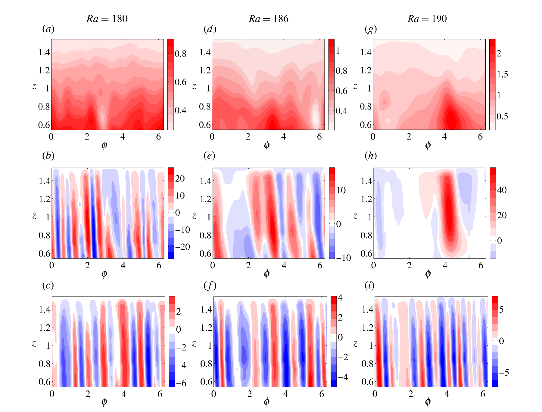
Figure 1: Cylindrical section ($z-\phi$) plots within the tangent cylinder of the $z$-magnetic field (top panels), dynamo $z$-velocity (centre panels) and non-magnetic $z$-velocity (bottom panels), for $E=5\times 10^{-5}$, $Pr=Pm=5$ and three Rayleigh numbers $Ra$ near onset of magnetic convection. No-slip, electrically insulating boundaries are used. The plots are shown at cylinder radii $s=0.33$ (a,b), $s=0.18$ (d,e), $s=0.21$ (g,h) and $s=0.3$ (c,f,i).

For $E=5\times 10^{-6}$, convection outside the tangent cylinder starts at $Ra=50.18$. Figure 2(b) shows that at $Ra=385$, small-scale convection is uniformly distributed inside the tangent cylinder. A comparison of the $z$-velocities in the dynamo and non-magnetic runs (figure 2b,c) shows that the magnetic field intensifies the flow even as its small-scale structure is preserved. The scale of the lateral variation of $B_{z}$ seen in figure 2(d) ($Ra=415$) is fixed by the pre-existing small-scale velocity field interacting with the field diffusing from outside the tangent cylinder, and this can explain why the transverse lengthscale of $B_{z}$ is appreciably smaller compared to that at the higher Ekman number. The small-scale patches of $B_{z}$ in turn concentrate small-scale $u_{z}$ over them, although convection is still active in other regions. The formation of isolated plumes causes a skewness in $u_{z}$, with the peak upwelling velocity being approximately twice the downwelling velocity (figure 2e). As $Ra$ is increased to 438, $B_{z}$ is strong enough to concentrate a small-scale plume over it and suppress convection elsewhere (figure 2g,h). The marked decrease in the azimuthal lengthscale of the plume with decreasing Ekman number (figures 1h and 2h) suggests that, while the plume is magnetically confined, its width (lengthscale perpendicular to the rotation axis, $L_{\perp}$) may be controlled by the fluid viscosity. As with the higher Ekman number, the non-magnetic simulations retain the uniformly distributed axial flow structure from the onset of convection (figure 2c,f,i).

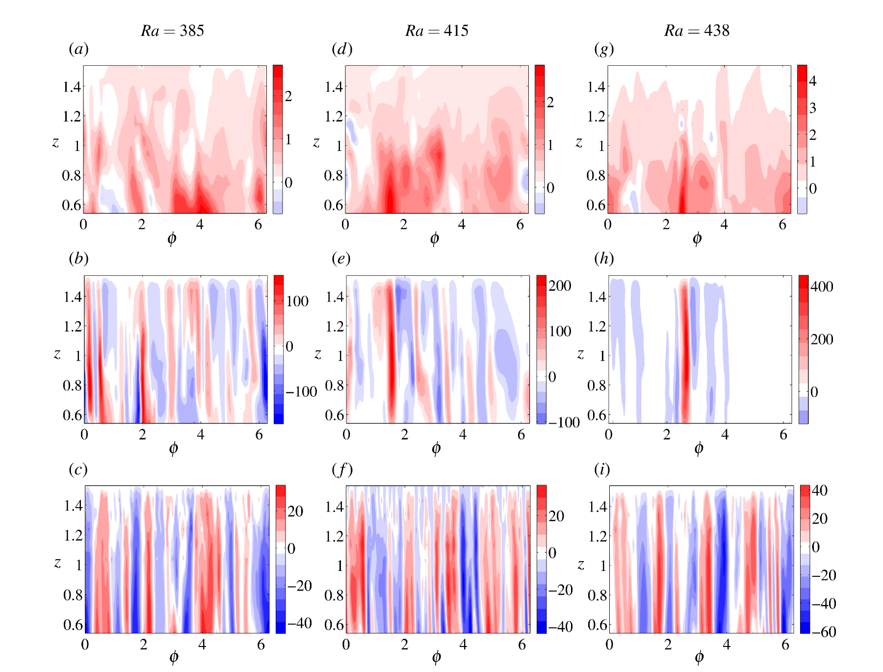
Figure 2: Cylindrical section ($z-\phi$) plots within the tangent cylinder of the $z$-magnetic field (top panels), dynamo $z$-velocity (centre panels) and non-magnetic $z$-velocity (bottom panels), for $E=5\times 10^{-6}$, $Pr=Pm=1$ and three Rayleigh numbers $Ra$ near onset of magnetic convection. No-slip, electrically insulating boundaries are used. The plots are shown at cylinder radii $s=0.35$ (a,b), $s=0.31$ (d,e), $s=0.33$ (g,h) and $s=0.3$ (c,f,i).

Figure 3 shows horizontal ($z$) section plots within the tangent cylinder of $B_{z}$ and $u_{z}$ for the two Ekman numbers at onset of the off-axis plume. The non-magnetic $u_{z}$ is provided for comparison. As $B_{z}$ is concentrated near the base of the convection zone, the strong correlation between the magnetic field and the flow is clearly visible by looking at two different sections, $z=0.9$ for $B_{z}$ and $z=1.4$ for $u_{z}$. The decrease in plume width $L_{\perp}$ at the lower Ekman number is evident by comparing the section plots of $u_{z}$ at the same $z$ (figure 3b,e). It is plausible that the magnetic field locally reduces the Rayleigh number for convection from its non-magnetic value, upon which the plume finds the location where the field is strongest. A strongly supercritical ($Ra=350$) dynamo simulation suggests that this idea deserves consideration, as the dominant upwelling in the tangent cylinder continuously migrates to the location of the peak magnetic field in a period of less than $\sim$ 0.1 magnetic diffusion time. Further studies at higher $Ra$ are necessary to obtain the regime where the $B_{z}$–$u_{z}$ correlation within the tangent cylinder completely breaks down.

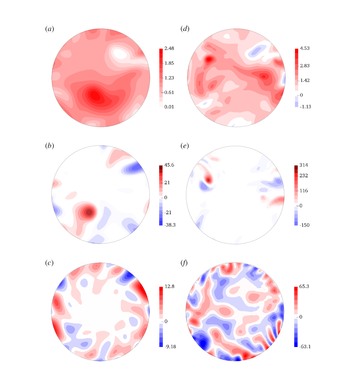
Figure 3: Horizontal ($z$) section plots within the tangent cylinder of the axial magnetic field $B_{z}$ at $z=0.9$ (top panel), the axial velocity $u_{z}$ for the dynamo at $z=1.4$ (centre panel) and $u_{z}$ for non-magnetic convection at $z=1.4$ (bottom panel). The periphery of these sections are at colatitude $21.04^{\circ}$ ($z=1.4$) and $30.9^{\circ}$ ($z=0.9$). The cylindrical radius in all plots is in the range $[0,0.5384]$ in dimensionless units. (a-c) $E=5\times 10^{-5}$, $Pr=Pm=5$, $Ra=190$; (d-f) $E=5\times 10^{-6}$, $Pr=Pm=1$, $Ra=438$. No-slip, electrically insulating boundary conditions are used.

Table 1 presents the parameters and some key properties of the dynamo simulations performed for the two Ekman numbers. The volume-averaged Elsasser number $\overline{B^{2}}$ ($\sim 1$ in all runs) does not give any insight into the onset of the localized plume in the tangent cylinder; on the other hand, the Elsasser number $\varLambda_{z}$ calculated based on the peak $B_{z}$ value in the tangent cylinder shows a clear increase at plume onset. The field components $B_{s}$ and $B_{\phi}$ are a factor $\approx 3$ lower than $B_{z}$.

$E$	$Ra$	$Rm$	$\overline{B^{2}}$	$\varLambda_{z}$
	180	66.19	0.9	1.34
$E=5\times 10^{-5}$	186	68.11	0.92	2.94
	190	68.58	0.97	3.49
	385	164.95	1.25	6.76
$E=5\times 10^{-6}$	415	181.81	1.39	7.92
	438	186.05	1.46	16.81

Table 1: Summary of the dynamo calculations for two Ekman numbers ($E$) at $q=1$ with no-slip, isothermal and electrically insulating boundary conditions. Here $Ra$ is the modified Rayleigh number, $Rm$ is the magnetic Reynolds number obtained from the root mean square (rms) value of the velocity and $\varLambda_{z}$ is the Elsasser number given by the square of the peak value of $B_{z}$ in the tangent cylinder.

A key issue that arises from the nonlinear dynamo simulations is whether the isolated plumes that form within the tangent cylinder are viscously or magnetically controlled. Although it may appear from the simulations at $E=5\times 10^{-5}$ that the magnetic field increases the scale of convection at plume onset (see figure 1b and h), a comparison across Ekman numbers shows that the plume width decreases with decreasing Ekman number (figure 3b,e). In addition, the Rayleigh number for plume onset within the tangent cylinder increases with decreasing Ekman number. These findings suggest that the onset of isolated plumes within the tangent cylinder is controlled by the fluid viscosity.

As the sloping boundaries (top and bottom caps) of the tangent cylinder themselves prevent perfect geostrophy, the critical Rayleigh number $Ra_{c}$ and wavenumber $k_{c}$ at which non-magnetic convection sets in may not be faithfully reproduced by a plane layer linear onset model. On the other hand, if a laterally varying magnetic field strongly localizes convection in the tangent cylinder, a plane layer magnetoconvection model could be a good approximation for the onset of magnetic convection in the tangent cylinder because the change of boundary curvature across a thin plume is small. Therefore, a study of convective onset in a plane layer under a laterally varying magnetic field is justified. This study is presented in the following section.

3 Linear magnetoconvection model

3.1 Problem set-up and governing equations

We consider an electrically conducting fluid in a plane layer of finite aspect ratio, where the vertical ($z$) and a horizontal ($x$) lengthscale are known and the third direction ($y$) is of infinite horizontal extent. The $z$ and $x$-directions mimic the axial ($z$) and azimuthal ($\phi$) directions in cylindrical polar coordinates $(s,\phi,z)$. The basic state temperature gradient across the layer sets up convection under gravity ${\bm{g}}$ that acts in the negative $z$ (downward) direction. The system rotates about the $z$-axis. The fluid layer is permeated by a laterally varying magnetic field of the form

$${\bm{B}}_{0}=\mathcal{B}_{0}f(x)\hat{\bm{z}};\,\,\,f(x)=a_{0}+a_{1}\exp\bigl{[}-(x-c)^{2}/2\delta^{2}\bigr{]},$$ (7)

where $\mathcal{B}_{0}$ is a reference magnetic field strength, $a_{0}$, $a_{1}$ and $c$ are constants and $\delta$ is the horizontal lengthscale of the magnetic field. The problem set-up is shown in figure 4.

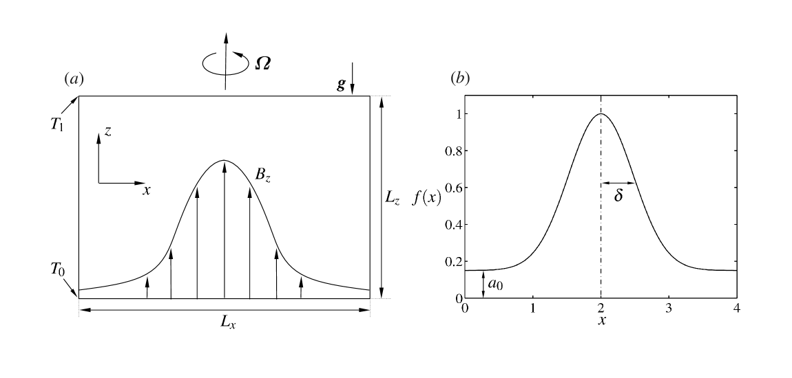
Figure 4: (a) Schematic of plane layer rotating magnetoconvection produced by a constant adverse temperature gradient under a laterally varying axial magnetic field. (b) The profile of $B_{0}$ in the layer from equation (7), with $a_{0}=0.15$, $a_{1}=0.85$, $c=2$ and $\delta=0.48$.

In the Boussinesq approximation, the following linearized MHD equations govern the system:

$$EPm^{-1}\frac{\partial\bm{u}}{\partial t}+\hat{\bm{z}}\times\bm{u}=-{\bm{\nabla}}p+\varLambda\bigl{[}({\bm{\nabla}}\times\bm{B}_{0})\times\bm{b}+({\bm{\nabla}}\times\bm{b})\times\bm{B}_{0}\bigr{]}$$

$$+PmPr^{-1}Ra\theta\hat{\bm{z}}+E\nabla^{2}\bm{u},$$ (8)

$$\frac{\partial\bm{b}}{\partial t}={\bm{\nabla}}\times(\bm{u}\times\bm{B}_{0})+\nabla^{2}\bm{b},$$ (9)

$$\frac{\partial\theta}{\partial t}=\bm{u}{\bm{\cdot}}\hat{\bm{z}}+PmPr^{-1}\nabla^{2}\theta,$$ (10)

$${\bm{\nabla}}{\bm{\cdot}}\bm{u}=\bm{\nabla}{\bm{\cdot}}\bm{b}=0,$$ (11)

The dimensionless parameters $E$, $Ra$, $Pm$ and $Pr$ in equations (8)–(10) have the same definitions as in (6), except that the spherical shell thickness $L$ is replaced by the plane layer depth $L_{z}$. The Elsasser number $\varLambda=\mathcal{B}_{0}^{2}/2\varOmega\rho\mu_{0}\eta$ is defined based on the reference magnetic field strength.

By applying the operators $({\bm{\nabla}}\times)$ and $({\bm{\nabla}}\times{\bm{\nabla}}\times)$ to the momentum equation (8) and $({\bm{\nabla}}\times)$ to the induction equation (9) and taking the $z$-components of the equations, the behaviour of the five perturbation variables – velocity, vorticity, magnetic field, electric current density and temperature – can be obtained. As the Roberts number $q$ is set to unity throughout this study, the onset of convection with an axial magnetic field is expected to be stationary for a wide range of Ekman numbers (Aujogue et al., 2015). Furthermore, this study aims to investigate the structure of convection at onset and seek comparisons with the long-time convection pattern within the tangent cylinder in saturated (quasi-steady) nonlinear dynamos. The time dependence of the perturbations is therefore not considered, and solutions are sought in the following form:

$$\bigl{[}u_{z}^{\prime},\omega_{z}^{\prime},b_{z}^{\prime},j_{z}^{\prime},\theta^{\prime}\bigr{]}(x,y,z)=\bigl{[}u_{z}(x,z),\omega_{z}(x,z),b_{z}(x,z),$$

$$j_{z}(x,z),\theta(x,z)\bigr{]}\exp\,(iky),$$ (12)

where $k$ is the wave number in the $y$-direction. After introducing this solution into the governing equations, the following system of differential equations is obtained:

$$E\bigl{(}D_{x}^{2}+D_{z}^{2}-k^{2}\bigr{)}^{2}u_{z}+\Lambda\bigl{[}f(x)\bigl{(}D_{x}^{2}+D_{z}^{2}-k^{2}\bigr{)}D_{z}b_{z}$$

$$+f^{\prime\prime}(x)D_{z}b_{z}+2f^{\prime\prime}(x)D_{x}b_{x}+f^{\prime}(x)D_{x}^{2}b_{x}+2f^{\prime}(x)D_{xz}^{2}b_{z}$$

$$+f^{\prime\prime\prime}(x)b_{x}-k^{2}f^{\prime}(x)b_{x}-f^{\prime}(x)D_{z}^{2}b_{x}\bigr{]}-D_{z}\omega_{z}-qRa\bigl{(}D_{x}^{2}-k^{2}\bigr{)}\theta = 0,$$ (13)

$$D_{z}u_{z}+\Lambda\bigl{(}f(x)D_{z}j_{z}+f^{\prime}(x)D_{z}b_{y}\bigr{)}+E\bigl{(}D_{x}^{2}+D_{z}^{2}-k^{2}\bigr{)}\omega_{z} = 0,$$ (14)

$$q\bigl{(}D_{x}^{2}+D_{z}^{2}-k^{2}\bigr{)}\theta+u_{z} = 0,$$ (15)

$$f(x)D_{z}u_{z}-f^{\prime}(x)u_{x}+\bigl{(}D_{x}^{2}+D_{z}^{2}-k^{2}\bigr{)}b_{z} = 0,$$ (16)

$$f(x)D_{z}\omega_{z}+f^{\prime}(x)D_{z}u_{y}+\bigl{(}D_{x}^{2}+D_{z}^{2}-k^{2}\bigr{)}j_{z} = 0,$$ (17)

where $D_{x}=\partial/\partial x$ and $D_{z}=\partial/\partial z$. The variables $u_{x}$, $u_{y}$, $b_{x}$, $b_{y}$ are related to the eigenfunctions $u_{z}$, $\omega_{z}$, $b_{z}$, $j_{z}$ by the identities

$$-[\nabla_{H}^{2}]u_{x} = D_{x}D_{z}u_{z}+ik\omega_{z},\,-[\nabla_{H}^{2}]u_{y}=ikD_{z}u_{z}-D_{x}\omega_{z},$$ (18)

$$-[\nabla_{H}^{2}]b_{x} = D_{x}D_{z}b_{z}+ikj_{z},\,\,\,-[\nabla_{H}^{2}]b_{y}=ikD_{z}b_{z}-D_{x}j_{z},$$ (19)

where $\nabla_{H}^{2}=D_{x}^{2}-k^{2}$ is the horizontal Laplacian.

The stability calculations are performed with both stress-free and no-slip boundaries on $z$. Electromagnetic conditions are insulating at the top and bottom, although one set of calculations with mixed (bottom perfectly conducting and top insulating) conditions is done to show that the nature of convective onset is not different from that for insulating walls. As isothermal conditions are maintained for the basic state, the temperature perturbation vanishes at the top and bottom. As the horizontal ($x$) direction mimics the azimuthal ($\phi$) direction in cylindrical polar coordinates, periodic conditions are set at the side walls. The boundary conditions on $z$ are implemented as follows:

$$u_{z}=D_{z}^{2}u_{z}=D_{z}\omega_{z}=0\ \,\, \text{at}\ z=0,1\ \text{(stress-free)};$$ (20)

$$u_{z}=D_{z}u_{z}=\omega_{z}=0\ \,\, \text{at}\ z=0,1\ \text{(no-slip)};$$ (21)

$$j_{z}=0\,\, \text{at}\ z=0,1\ \text{(both walls insulating)};$$ (22)

$$b_{z}=D_{z}j_{z}=0\,\, \text{at}\ z=0\ \text{(bottom wall conducting)};$$ (23)

$$\theta=0\,\, \text{at}\ z=0,1.$$ (24)

3.2 Method of solution and benchmarks

The stationary onset of magnetconvection with a laterally varying field is studied for the parameters $E=5\times 10^{-4}-5\times 10^{-7}$, $\varLambda=0-1$ and $q=1$. The generalized eigenvalue problem $\bm{AX}=\lambda\bm{BX}$, where $\lambda=Ra$ is solved using Matlab. For the set of equations (13)–(17), the matrices and their elements are presented in Appendix A. A spectral collocation method that uses Chebyshev differentiation in $z$ and Fourier differentiation in $x$ is used to resolve the eigenfunctions in two dimensions. For problems with variable coefficient terms (as in this study), the spectral collocation method uses simple matrix multiplication in physical space to treat the terms, whereas a pure spectral method would have resulted in convolution sums for such terms that are algebraically complex (Peyret, 2002). The drawback of the collocation method, however, is that the differentiation matrices are dense, making computations memory-intensive (Muite, 2010; Hu et al., 2012). The construction of the Fourier and Chebyshev differentiation matrices follows a standard approach, and is given in Appendix A for completeness. For $E=5\times 10^{-7}$ with stress-free boundaries, grid independence is secured with $18$ points in $z$ and $210$ points in $x$, so the non-zero elements of ${\bm{A}}$ and ${\bm{B}}$ are of size $(18\times 210)^{2}$.

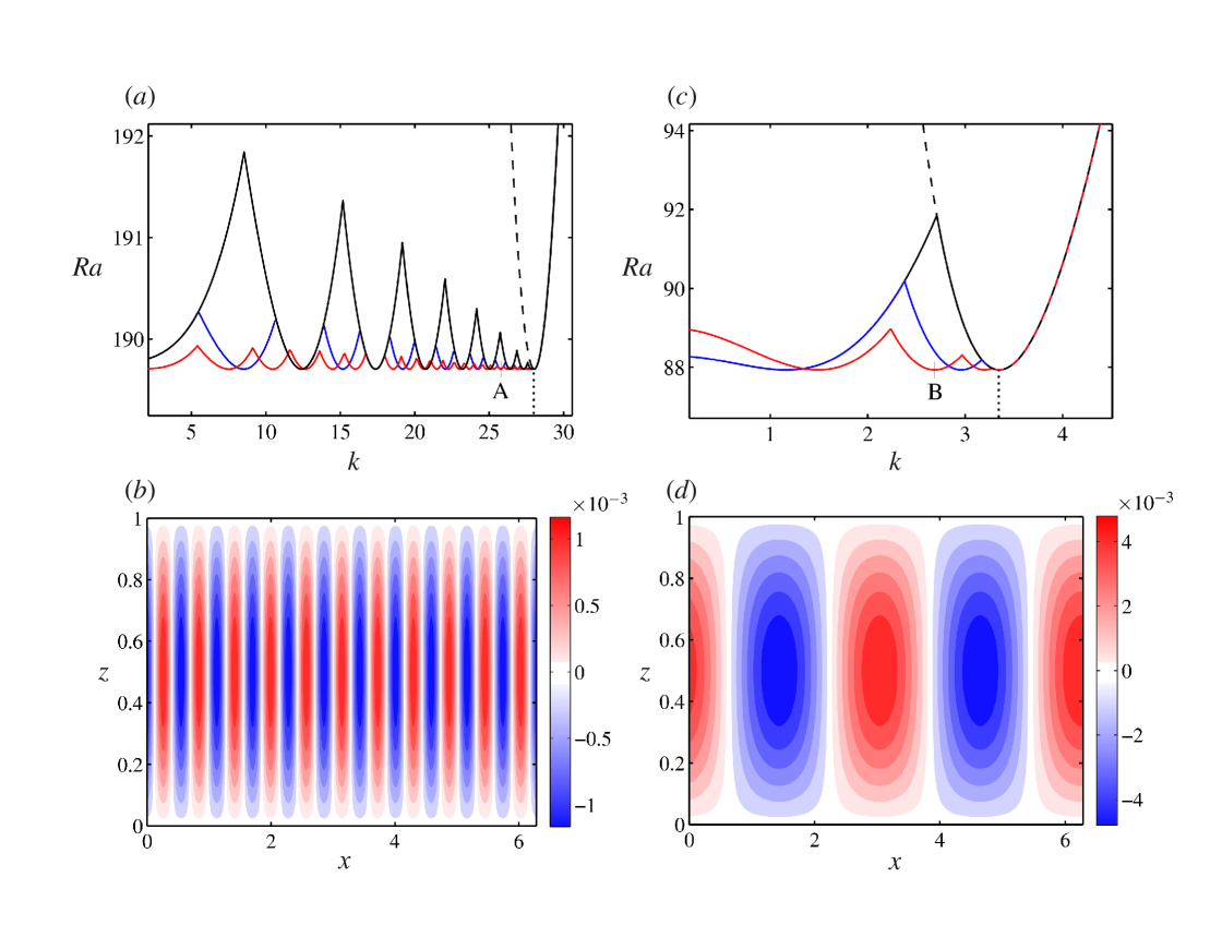
Figure 5: (a) Neutral stability curves for non-magnetic convection in a plane layer of finite aspect ratio for $E=1\times 10^{-4}$ and stress-free $z$-boundaries. The cases shown are $L_{x}=2$ (black), $L_{x}=4$ (blue) and $L_{x}=2\pi$ (red). (b) Axial velocity ($u_{z}$) for the unstable mode marked ‘A’ ($L_{x}=2\pi,k=25.78$) in (a). (c) Neutral stability curves for magnetoconvection at $E=1\times 10^{-4}$, $\varLambda=0.5$ and $q=1$, for the same cases (and line styles) as (a). (d) $u_{z}$ for the unstable mode marked ‘B’ ($L_{x}=2\pi,k=2.69$) in (c). The dashed lines in (a) and (c) are the neutral curves for the infinite plane layer. The layer depth $L_{z}=1$ in all cases.

Figure 5 shows the existence of a finite number of equally unstable $y$-wavenumbers ($k$) at the onset of convection in a plane layer of finite aspect ratio. The exact number and values of the unstable wavenumbers are predictable for a given horizontal lengthscale $L_{x}$ (Appendix B). As $L_{x}\to\infty$, the number of unstable wavenumbers would become infinite. For a given $L_{x}$,

$$a^{2}=\biggl{(}\frac{2m\pi}{L_{x}}\biggr{)}^{2}+k^{2},$$

where $m$ is the $x$-wavenumber and $a$ is the resultant wavenumber. Consequently, the last unstable $y$-wavenumber coincides with the critical wavenumber $a_{c}$ for the classical one-dimensional plane layer of infinite horizontal extent (Chandrasekhar, 1961). For $E=1\times 10^{-4}$, non-magnetic convection gives $a_{c}=28.02$; and for $L_{x}=2\pi$, the axial velocity $u_{z}$ at the unstable wavenumber marked A in figure 5(a) shows 11 pairs of rolls (figure 5b), consistent with the fact that $m_{c}=\sqrt{28.02^{2}-25.78^{2}}\approx 11$. In a similar way, convection under a uniform axial magnetic field for $E=1\times 10^{-4}$ and $\varLambda=0.5$ at the point B in figure 5(c) produces 2 pairs of rolls (figure 5d) because $a_{c}=3.35$ and $m_{c}=\sqrt{3.35^{2}-2.69^{2}}\approx 2$.

3.3 Onset of convection under a laterally varying magnetic field

We investigate marginal-state convection in a plane layer of depth $L_{z}=1$ and horizontal lengthscale $L_{x}=4$ permeated by an inhomogeneous axial ($z$) magnetic field of the form (7) giving strong localization of the field (see figure 4b). The background value of the field is small compared to its peak value but not zero, in line with the axial field distribution within the tangent cylinder in rapidly rotating dynamo simulations. Figures 6 and 7 give the critical Rayleigh number ($Ra_{c}$) and wavenumber ($k_{c}$) diagrams for this field distribution, with the reference states for non-magnetic convection and homogeneous magnetic field provided for comparison. The critical wavenumber for the homogeneous field is not shown because its value is not unique, as noted earlier in §3.2 (although the critical resultant wavenumber $a_{c}$ is unique). For the laterally varying field, $Ra_{c}$ follows the same trend as for the homogeneous field, being approximately constant in the large-wavenumber viscous branch and then falling steeply in the small-wavenumber magnetic branch. The field inhomogeneity, however, displaces the viscous–magnetic mode transition point to a higher Elsasser number. Changing the mechanical and electromagnetic $z$-boundary conditions does not alter the basic properties of the regime diagrams, although the numerical values of $Ra_{c}$ and $k_{c}$ differ from one condition to the other. While the viscous branches for insulating and mixed (top insulating and bottom perfectly conducting) electromagnetic conditions largely overlap, the use of mixed conditions moves the viscous–magnetic transition further to the right (compare the blue and magenta lines in figure 6a and b). Table 2 (for stress-free conditions) and table 3 (for no-slip conditions) present selected values of the critical parameters spanning the two branches of instability. A notable property of onset in the magnetic mode is that $Ra_{c}$ and $k_{c}$ are nearly independent of the Ekman number $E$, in agreement with the classical picture of onset in an infinite plane layer under a uniform magnetic field (see, for example, figure 3 in Aujogue et al., 2015). In this regime, the critical temperature gradient for convection is independent of viscosity, and it is the magnetic field via the Lorentz force that breaks the Taylor-Proudman constraint to set up convection in the fluid layer.

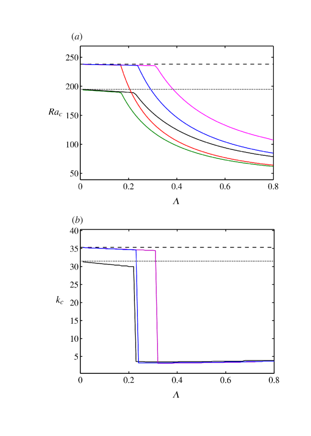
Figure 6: $Ra_{c}$ – $\varLambda$ and $k_{c}$ – $\varLambda$ regime diagrams for $E=5\times 10^{-5}$. The reference values for the non-magnetic case ($\varLambda=0$) are given by the horizontal dashed (stress-free) and dotted (no-slip) lines. The uniform magnetic field cases are given by red (stress-free and insulating) and green (no-slip and insulating) lines. The inhomogeneous magnetic field cases are given by blue (stress-free and insulating), magenta (stress-free and mixed) and black (no-slip and insulating) lines.

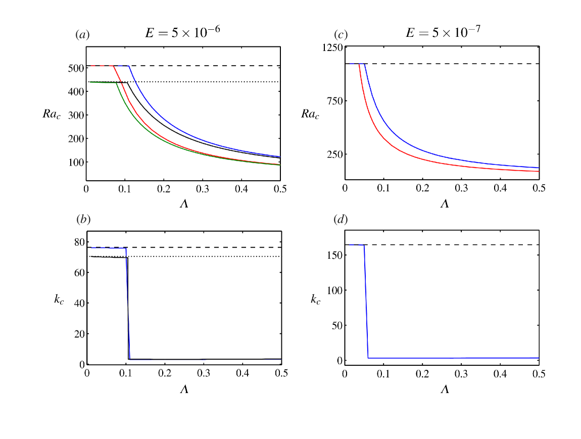
Figure 7: $Ra_{c}$ – $\varLambda$ and $k_{c}$ – $\varLambda$ regime diagrams for $E=5\times 10^{-6}$ and $E=5\times 10^{-7}$. The reference values for the non-magnetic case ($\varLambda=0$) are given by the horizontal dashed (stress-free) and dotted (no-slip) lines. The uniform magnetic field cases are given by red (stress-free and insulating) and green (no-slip and insulating) lines. The inhomogeneous field cases are given by blue (stress-free and insulating) and black (no-slip and insulating) lines.

$E=5\times 10^{-5}$				$E=5\times 10^{-6}$			$E=5\times 10^{-7}$
(Stress-free)				(Stress-free)			(Stress-free)
$\varLambda$	$Ra_{c}$	$k_{c}$		$\varLambda$	$Ra_{c}$	$k_{c}$		$\varLambda$	$Ra_{c}$	$k_{c}$
0	237.91	35.35		0	509.41	76.27		0	1096	164.38
0.001	237.83	35.3		0.001	509.37	76.25		0.001	1095.97	164.3
0.01	237.82	35.3		0.01	509.30	76.1		0.01	1095.90	164.3
0.04	237.57	35.1		0.04	509.01	76.1		0.04	1095.72	164.1
0.1	237.03	35		0.1	508.43	75.9		0.05	1095.61	164.1
0.2	236.10	34.7		0.11*	507.73	3.1; 75.9		0.051	1095.22	3.06
0.22	235.90	34.6		0.12	465.91	3.08		0.1	560.33	3.07
0.238*	235.70	3.2; 34.6		0.15	374.14	3.09		0.15	375.23	3.08
0.239	233.44	3.16		0.2	282.61	3.11		0.2	283.37	3.1
0.3	189.01	3.2		0.3	191.92	3.17		0.3	192.20	3.16
0.5	120.58	3.35		0.5	121.62	3.35		0.5	121.73	3.35
0.6	104.29	3.5		0.6	105.01	3.48		0.6	105.08	3.48
0.8	85.28	3.8		0.8	85.68	3.78		0.8	85.72	3.78
1.0	75.33	4.15		1.0	75.57	4.13		1.0	75.60	4.13

Table 2: Rayleigh numbers ($Ra_{c}$) and wavenumbers ($k_{c}$) for marginal state (critical) convection, computed for Elsasser numbers ($\varLambda$) in the range 0–1 and stress-free $z$-boundaries. *Denotes the viscous–magnetic mode transition point.

$E=5\times 10^{-5}$				$E=5\times 10^{-6}$
(No-slip)				(No-slip)
$\varLambda$	$Ra_{c}$	$k_{c}$		$\varLambda$	$Ra_{c}$	$k_{c}$
0	194.65	31.3		0	440.82	70.5
0.001	194.61	31.3		0.001	440.81	70.4
0.01	194.56	31.3		0.01	440.80	70.4
0.04	193.80	31.1		0.04	439.73	70
0.1	192.21	30.7		0.1	437.45	69.6
0.15	190.87	30.4		0.107*	436.91	3.3; 69.6
0.2	189.50	30		0.11	424.03	3.3
0.225*	188.78	3.6; 30		0.2	256	3.2
0.23	185.95	3.6		0.3	179.78	3.3
0.3	154.15	3.5		0.4	140.42	3.3
0.5	106.54	3.5		0.5	116.83	3.4
0.6	93.99	3.6		0.6	101.41	3.5

Table 3: Rayleigh numbers ($Ra_{c}$) and wavenumbers ($k_{c}$) for marginal state (critical) convection, computed for Elsasser numbers ($\varLambda$) in the range 0–0.6 and no-slip $z$-boundaries. *Denotes the viscous–magnetic mode transition point.

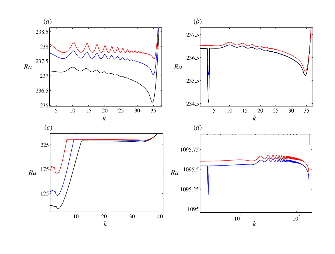
Figure 8: Neutral stability curves for different magnitudes of the imposed inhomogeneous magnetic field in figure 4(b) and stress-free, electrically insulating $z$-boundaries. Two Ekman numbers are analyzed, $E=5\times 10^{-5}$ (a–c) and $E=5\times 10^{-7}$ (d). (a) $\varLambda=0.04$ (red), $\varLambda=0.1$ (blue), $\varLambda=0.2$ (black). (b) $\varLambda=0.22$ (red), $\varLambda=0.238$ (blue), $\varLambda=0.239$ (black). (c) $\varLambda=0.3$ (red), $\varLambda=0.5$ (blue), $\varLambda=0.7$ (black). (d) $\varLambda=0.04$ (red), $\varLambda=0.051$ (blue).

Figure 8 presents the neutral stability curves extracted from various points on the regime diagrams for two Ekman numbers. For $E=5\times 10^{-5}$, the laterally varying magnetic field of small strength $\varLambda=0.04$ forces a unique mode of instability ($k_{c}=35.1$), even as the vestige of the multiple-wavenumber, non-magnetic solution is visible in the oscillations of the curve (figure 8(a), red line). The amplitude of the oscillations decreases with increasing Elsasser number, and for $\varLambda=0.238$ (blue line in figure 8b), the magnetic mode of onset ($k_{c}=3.2$) appears at the same Rayleigh number as the viscous mode ($k_{c}=34.6$). For $\varLambda=0.239$, the magnetic mode overtakes the viscous mode as the most unstable. As $\varLambda$ is increased further, $Ra_{c}$ progressively decreases but $k_{c}$ remains approximately constant (figure 8c). The viscous–magnetic mode transition at $E=5\times 10^{-7}$ takes place over a very narrow range of Elsasser numbers, with $\varLambda=0.05$ showing viscous onset ($k_{c}=164.1$) and $\varLambda=0.051$ showing magnetic onset ($k_{c}=3.06$; blue line in figure 8d). (The logarithmic $x$-axis scale of figure 8(d) shows the large scale separation between the viscous and magnetic modes clearly). The large-wavenumber oscillations still exist, although with the laterally varying magnetic field these are never the most unstable modes.

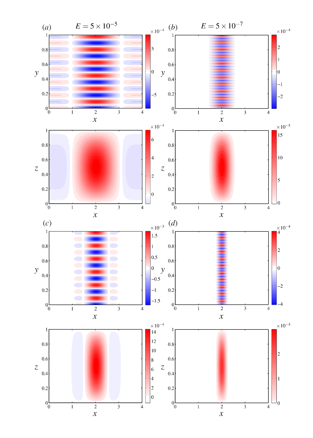
Figure 9: Contour plots of the axial velocity $u_{z}$ for two Ekman numbers ($E$) at onset of magnetoconvection on the $(x,z)$ and $(x,y)$ planes, with a restricted $y$-range of $[0,1]$. (a) and (b): $\varLambda=10^{-3}$. (c) and (d): $\varLambda=0.04$. The $z$-boundaries are stress-free and electrically insulating.

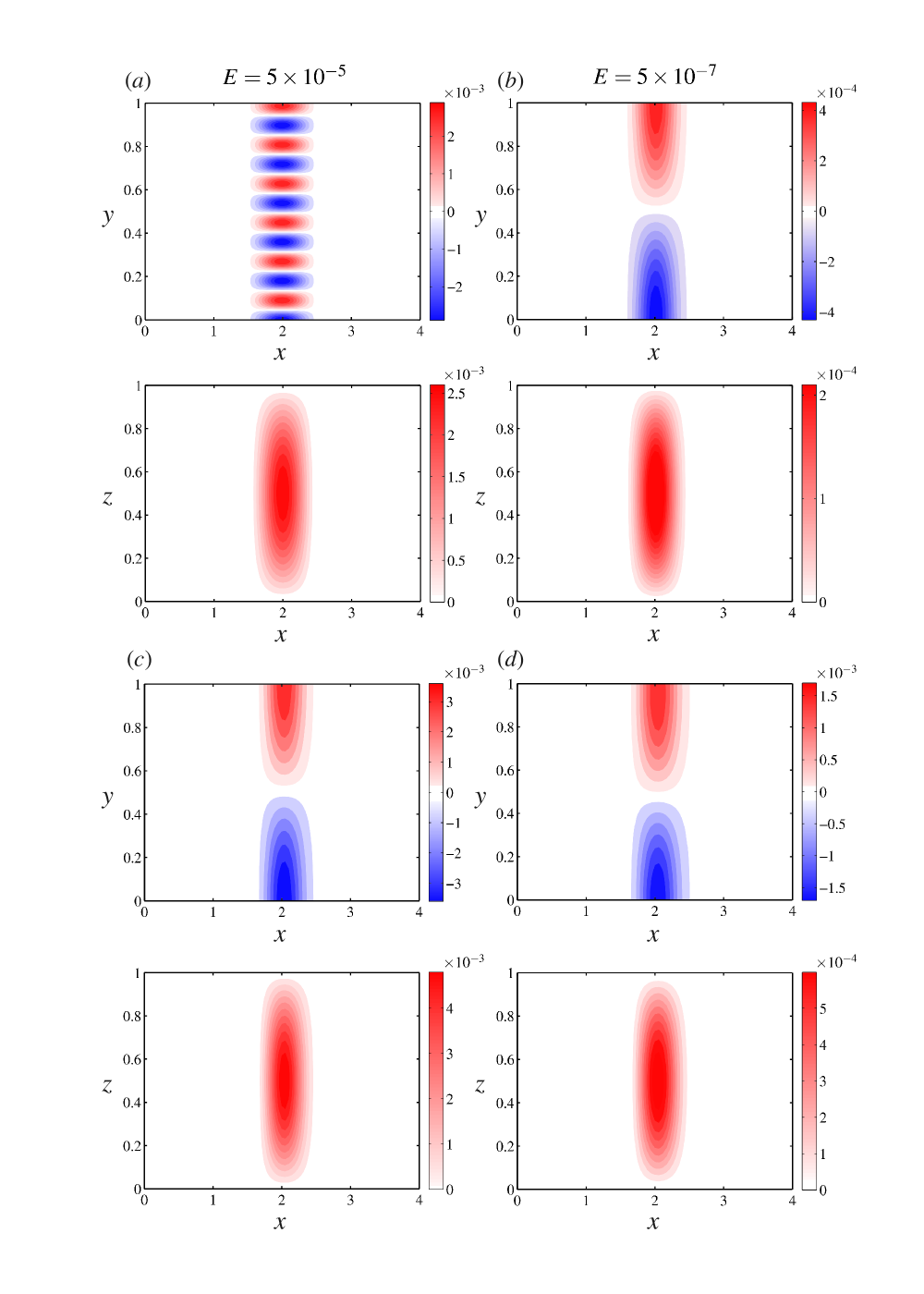
Figure 10: Axial velocity $u_{z}$ for two Ekman numbers ($E$) at onset of magnetoconvection on the $(x,z)$ and $(x,y)$ planes. (a) and (b): $\varLambda=0.1$. (c) and (d): $\varLambda=0.3$. The $z$-boundaries are stress-free and electrically insulating.

Figures 9 and 10 show the axial velocity $u_{z}$ at convective onset for two Ekman numbers. (Both $u_{z}$ and $\theta$ have identical structures.) The main idea that comes out of this study is that convection takes the form of isolated plumes under a laterally varying magnetic field even when the smallest lengthscale of the flow is controlled by viscosity. For a small field strength $\varLambda=10^{-3}$, a unique mode of instability develops where convection is concentrated in the neighbourhood of the peak magnetic field at $x=2$ (figures 9a,b). (It has been confirmed that moving the peak location of the imposed field by changing the constant $c$ in equation (7) also moves the location of convection). The large number of convection cells stacked in the $(x,y)$ plane points to the viscous mode of onset. Convection here is magnetically confined, yet its smallest lengthscale is viscously controlled. The magnetic field can therefore help overcome the Taylor-Proudman constraint and set up localized convection while not significantly changing the wavenumber of convection from its non-magnetic value. It is notable that the field-induced localization is more pronounced at the lower Ekman number: for $\varLambda=10^{-3}$ and $\varLambda=0.04$, the rolls at $E=5\times 10^{-7}$ are appreciably thinner than at $E=5\times 10^{-5}$, although the imposed magnetic field profile is the same in both cases (figures 9a and b; 9c and d). The formation of thin, yet isolated plumes has direct relevance to convection within the tangent cylinder in rapidly rotating spherical dynamo simulations (§2) where similar structures are noted. As the field strength is increased further to $\varLambda=0.1$, convection at $E=5\times 10^{-5}$ is still in the large-wavenumber viscous branch, whereas convection at $E=5\times 10^{-7}$ has crossed over to the small-wavenumber magnetic branch (figures 10(a) and (b) and table 2). From figures 10(c) and (d) ($\varLambda=0.3$), it is noted that the small-wavenumber convection at both Ekman numbers is almost identical in structure, consistent with the fact that the critical parameters ($Ra_{c}$, $k_{c}$) are independent of Ekman number beyond the viscous–magnetic transition point (e.g. Aujogue et al., 2015).

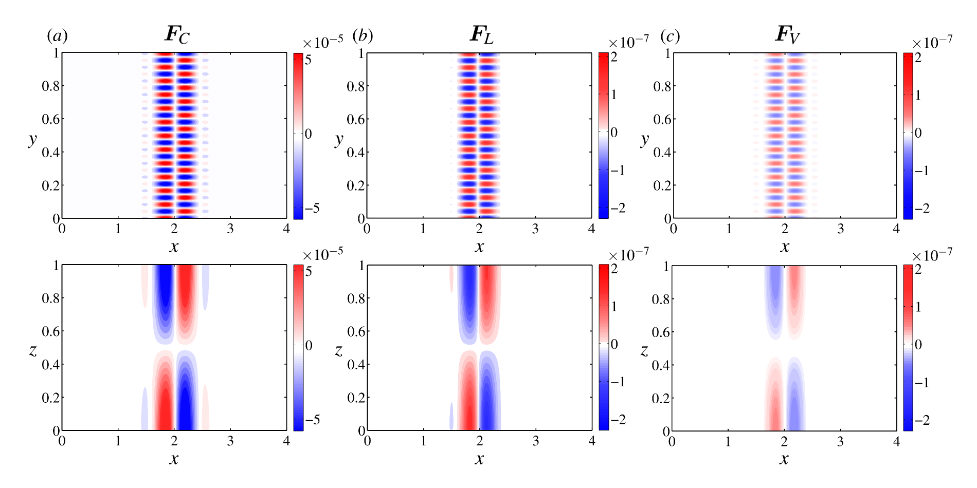
Figure 11: Contour plots of the $x$-components of the Coriolis force $\bm{F}_{C}$, Lorentz force $\bm{F}_{L}$ and viscous force $\bm{F}_{V}$ on the $(x,z)$ and $(x,y)$ planes. The $(x,z)$ plane is shown at $y=0$. The parameters are $E=5\times 10^{-6}$ and $\varLambda=0.08$. The $z$-boundaries are stress-free and electrically insulating.

Figure 11 shows the $x$-components of the Coriolis, Lorentz and viscous forces (denoted by subscripts $C$, $L$ and $V$ respectively) in the momentum equation (8). (In this model, the pressure gradient is not solved for). Here $E=5\times 10^{-6}$, for which $\varLambda=0.08$ gives onset in the viscous branch (table 2). The $x$-component of $\bm{F}_{C}$ gives $u_{y}$. From the plots of the Lorentz and viscous forces shown on the same colour scale (figure 11b,c), it is inferred that the Lorentz force, whose magnitude is $\approx 5$ times that of the viscous force, is influential in overcoming the Taylor-Proudman constraint and setting up convection. Interestingly, $\varLambda\bigl{[}(\bm{\nabla}\times\bm{b})\times\bm{B}_{0}\bigr{]}$ makes the dominant contribution to the Lorentz force while $\varLambda\bigl{[}(\bm{\nabla}\times\bm{B}_{0})\times\bm{b}\bigr{]}$ is slightly smaller in magnitude than the viscous force $E\nabla^{2}\bm{u}$ (see equation 8). At onset in the magnetic branch ($\varLambda=0.3$), the peak value of $\bm{F}_{L}$ is three orders of magnitude larger than that of $\bm{F}_{V}$ and only one order of magnitude smaller than that of $\bm{F}_{C}$, which emphasizes the well-known role of the magnetic field in overcoming the rotational constraint.

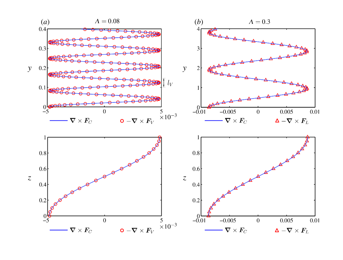
Figure 12: Line plots at $x=2$ showing the principal balance of terms in the $z$-vorticity equation for two values of $\varLambda$ that represent the viscous and magnetic modes of onset. The $z$-variation is shown at $y=0$. The Ekman number $E=5\times 10^{-6}$. The $z$-boundaries are stress-free and electrically insulating.

The mode of convective onset is reflected in the principal balance of terms in the $z$-vorticity equation (14). For $\varLambda=0.08$, $\bm{\nabla}\times{\bm{F}}_{C}$ closely matches $-\bm{\nabla}\times{\bm{F}}_{V}$ (figure 12a), whereas for $\varLambda=0.3$, $\bm{\nabla}\times{\bm{F}}_{C}$ closely matches $-\bm{\nabla}\times{\bm{F}}_{L}$ (figure 12b). The Lorentz force term has a negligible contribution to the balance in the former case while the viscous force term has a negligible effect in the latter. The $y$-axis range for the two cases is chosen such that the difference in the lengthscale of convection is clear. Although the large-scale magnetic mode of onset in figure 12(b) is well understood, the role of the Lorentz force in setting up convection at the small viscous lengthscale $l_{V}$ (figure 12a, upper panel) has not received much attention in the literature.

Increasing the background magnetic field intensity relative to the peak value reduces the lateral inhomogeneity of the field. For moderate lateral variation, obtained by progressively increasing $a_{0}$ in the mean field profile (7), convection at onset retains the structure of isolated rolls centered at the location of the peak field. A weak lateral variation ($a_{0}\sim 0.8$), however, gives rise to a cluster of rolls in the viscous mode whose intensity decays from the centre ($x=2$) towards the periphery. As the lateral variation goes to zero, the solution would tend to that for a homogeneous magnetic field (§3.2).

In summary, a laterally varying magnetic field acting on a rotating fluid layer gives rise to a unique mode of instability where convection follows the path of the peak field. This localized excitation of convection is consistent with the idea that the magnetic field generates helical fluid motion in regions that are otherwise quiescent (Sreenivasan & Jones, 2011), although here it is shown that the flow lengthscale at onset could be viscously or magnetically controlled. The critical Rayleigh number for magnetic convection increases with decreasing Ekman number in the viscous branch of onset, whereas it is nearly independent of Ekman number in the magnetic branch. The width of the convection zone decreases with decreasing Ekman number in the viscous branch, whereas it is nearly independent of Ekman number in the magnetic branch.

3.4 Implications for onset of localized convection within the tangent cylinder

From a comparison between the plane layer linear magnetoconvection model and the spherical shell dynamo simulations, the following points are noted:

1. The Rayleigh number for onset of localized convection (in the form of an isolated plume) within the tangent cylinder ($Ra=190$ for $E=5\times 10^{-5}$ and $Ra=438$ for $E=5\times 10^{-6}$, with no-slip boundaries) lies on the viscous branch of onset in the plane layer magnetoconvection model ($Ra_{c}=194.6$–$188.8$ for $E=5\times 10^{-5}$ and $Ra_{c}=440.8$–$436.9$ for $E=5\times 10^{-6}$, with no-slip boundaries). This agreement between the plane layer and the spherical dynamo Rayleigh numbers rests on two factors: (a) The dominant magnetic field within the tangent cylinder is axial; and (b) the formation of localized convection within the tangent cylinder is practically unaffected by the curvature of the bounding walls. It is notable that the plane layer model does not predict the critical Rayleigh number for non-magnetic convection in the tangent cylinder, as the sloping walls allow uniformly distributed convection at a lower Rayleigh number (e.g. $Ra\sim 140$ for $E=5\times 10^{-5}$).

2. The width of an isolated plume within the tangent cylinder markedly decreases with decreasing Ekman number (figure 3b,e), an effect that is noted only in the viscous branch of onset in the magnetoconvection model (figure 9c,d). Had the plume formed in the magnetic branch of onset, its width should have been nearly independent of the Ekman number (figure 10c,d).

The close agreement between the dynamo and viscous-branch magnetoconvection Rayleigh numbers notwithstanding, the critical Elsasser number $\varLambda_{z}$ in the simulation is much higher than that in the linear magnetoconvection model. For example, in the dynamo simulation at $E=5\times 10^{-6}$, plume onset occurs for $\varLambda_{z}\approx 16.8$ while $Ra$ does not depart much from its nonmagnetic value with no-slip boundaries, $440.82$ (see tables 1 and 3). This striking difference in $\varLambda_{z}$ between the spherical shell tangent cylinder and the plane layer model is because of the naturally occurring axial variation of $B_{z}$ (e.g. figure 2c) whose effect is not considered in the layer model. A recent study (Gopinath & Sreenivasan, 2015) shows that a horizontal magnetic field of small axial lengthscale (more applicable to convection outside the tangent cylinder than inside) shifts the viscous–magnetic mode transition point from the classical value for a uniform field, $\varLambda=O(E^{1/3})$ to a much higher value $O(1)$, without a drastic change in the critical Rayleigh number. It is therefore possible that this transition point is displaced to large $\varLambda_{z}$ for an axially varying $B_{z}$, allowing an intense, spatially varying magnetic field to exist for $\overline{B^{2}}\sim 1$. Linear magnetoconvection with field variation along the axial coordinate $z$ (in addition to $x$, $y$ or both) brings additional complexities owing to the presence of a horizontal field component required to satisfy the divergence-free condition of the mean field, and the presence of a mean flow arising from the Magnetic–Coriolis force balance in the vorticity equation. Nevertheless, such a model is useful in predicting the $z$-magnetic field intensity required to produce isolated plumes within the tangent cylinder.

4 Concluding remarks

The new results that have come out of this study are summarized below in points (i)–(iv), together with what was known from earlier studies:

1. A comparison across Ekman numbers of the onset of an isolated plume within the tangent cylinder in dynamo simulations reveals that (a) the Rayleigh number for plume onset increases with decreasing $E$, and (b) the plume width markedly decreases with decreasing $E$. These results bear the hallmark of viscous-mode convection. In addition, the strong $B_{z}$–$u_{z}$ correlation suggests that the plume may seek out the location where the field is strongest.

   Earlier studies (§1) proposed that the tangent cylinder plume is in the large-scale magnetic mode, in which case its onset Rayleigh number and width should be independent of $E$. However, these studies did not examine plume onset across Ekman numbers.

2. A laterally varying axial magnetic field localizes convection in a rotating plane layer. The onset of convection takes the form of isolated plumes in regions where the magnetic field is strong. Of particular interest is the onset of localized, small-scale convection (e.g. figure 9(c), for $\varLambda=0.04$ and $E=5\times 10^{-5}$), in which case the critical Rayleigh number $Ra_{c}$ is not significantly different from that for non-magnetic convection (figure 6(a), blue line).

   Earlier onset models (see §1) did not consider the possibility of a laterally varying mean field locally exciting convection in a rotating layer. These models predicted uniformly distributed convection either in the small-scale viscous mode or in the large-scale magnetic mode, with the viscous–magnetic transition occurring at $\varLambda=O(E^{1/3})$.

3. The Rayleigh number for plume onset within the tangent cylinder agrees closely with the viscous-mode Rayleigh number in the plane layer magnetoconvection model (§3.4). This result suggests that the localized convection within the tangent cylinder is in the viscous mode.

4. It follows from (iii) that the onset of an isolated plume within the tangent cylinder is approximately linear, even as nonlinear dynamo action exists outside the tangent cylinder.

   While it is already known that the onset of pure (non-magnetic) convection inside the tangent cylinder requires a Rayleigh number much higher than the critical Rayleigh number outside it, our study provides an analogous result for magnetic convection.

Since the confinement of convection occurs in both viscous and magnetic modes of onset and the plume width increases at the mode cross-over point (figures 9d and 10b), it might appear that a strong magnetic field within the tangent cylinder would give rise to a plume in the magnetic mode. Notably, however, the plume width does not increase with increasing $Ra$ (and $\varLambda_{z}$) in the dynamo regime of relatively strong rotation ($E=5\times 10^{-6}$; figure 2). This indicates that the effect of rotation on the plume width prevails over the effect of the magnetic field, so that the viscous–magnetic mode transition does not occur. It is hence reasonable to suppose that the laterally varying field within the Earth’s tangent cylinder would strongly localize plumes in the small-scale viscous mode, in turn producing non-axisymmetric polar vortices. The width of plumes is likely determined by the smallest scale that can be supported against magnetic diffusion in the core; it is plausible that this scale has magnetic Reynolds number $Rm\sim 1$.

The nonlinear dynamo simulations in this study are far from the low-$E$, low-$q$ regime thought to exist in the Earth’s core. Simulations in which magnetic diffusion is significantly higher than thermal (and viscous) diffusion would help ascertain whether the critical Rayleigh number for plume formation progressively increases or tends to an asymptotic value as $E$ is decreased.

The linear stability analysis makes the simplifying assumption that the imposed field is invariant along one of the horizontal directions ($y$) that is chosen to be infinite in extent. The three-dimensional linear simulation of the case in figure 9(c) with the field varying in both $x$ and $y$ shows that the confinement in the $x$-direction is merely replicated in the $y$-direction with no change in the critical Rayleigh number ($Ra_{c}\approx 237.6$). Whereas decomposing the perturbations as waves along $y$ involves no loss of generality, it offers two distinct advantages: The critical $y$-wavenumber ($k_{c}$) readily confirms whether convection is viscously or magnetically controlled; and the calculations are far less expensive than three-dimensional onset simulations. Calculations for $E<5\times 10^{-7}$ are memory-intensive with the spectral collocation method, but the evolution of pure spectral methods may eventually overcome this limitation.

The confinement of rotating convection at small Elsasser number does not imply that the mean magnetic field strength within the Earth’s tangent cylinder should be small. Rather, a field strength of $\varLambda_{z}\sim 10$ or higher is plausible (table 1). Consideration of the axial inhomogeneity of the magnetic field would likely displace the viscous–magnetic mode cross-over point to much higher $\varLambda_{z}$, which makes small-scale convection a reality for intense, spatially varying fields. Despite the naturally occurring $z$-variation of the axial field inside the tangent cylinder, the Rayleigh number for plume onset matches well with the approximately constant Rayleigh number for viscous magnetoconvection. This indicates that the main effect of the $z$-variation is to extend the viscous regime to higher Elsasser numbers.

Binod Sreenivasan thanks the Department of Science and Technology (Government of India) for the award of a SwarnaJayanti Fellowship.

Appendix A Matrices for linear magnetoconvection in two dimensions

The problem given by equations (13)–(17) is of the form $\bm{AX}=\lambda\bm{BX}$, where

$$\bm{A} = \begin{pmatrix}\begin{array}[]{ccccc}ED^{4}&-I_{x}\otimes D_{z}&0&a_{14}&a_{15}\\ I_{x}\otimes D_{z}&ED^{2}&0&a_{24}&a_{25}\\ I&0&qD^{2}&0&0\\ a_{41}&f^{\prime}(x)I(ikH)&0&D^{2}&0\\ a_{51}&a_{52}&0&0&D^{2}\end{array}\end{pmatrix},\,\,\bm{X}=\begin{pmatrix}\begin{array}[]{c}u_{z}\\ \omega_{z}\\ \theta\\ b_{z}\\ j_{z}\end{array}\end{pmatrix},$$

$$\bm{B} = \begin{pmatrix}\begin{array}[]{ccccc}0&0&-q(D_{x}^{2}\otimes I_{z}-k^{2}I)&0&0\\ 0&0&0&0&0\\ 0&0&0&0&0\\ 0&0&0&0&0\\ 0&0&0&0&0\end{array}\end{pmatrix},\,\,\lambda=Ra.$$ (25)

Here $I_{x}$ and $I_{z}$ are identity matrices of size $N_{x}\times N_{x}$ and $N_{z}\times N_{z}$ respectively ($N_{x}$ and $N_{z}$ being the number of points in $x$ and $z$), so that $I=I_{x}\otimes I_{z}$ has size $(N_{x}\times N_{z})^{2}$.

The differential operator matrices in (25) are given by

$$D^{2} =D_{x}^{2}\otimes I_{z}+I_{x}\otimes D_{z}^{2}-k^{2}I,$$ (26)

$$D^{4} =D_{x}^{4}\otimes I_{z}+k^{4}I+I_{x}\otimes D_{z}^{4}-2k^{2}D_{x}^{2}\otimes I_{z}$$

$$\quad-2k^{2}I_{x}\otimes D_{z}^{2}+2D_{x}^{2}\otimes D_{z}^{2},$$ (27)

$$H =[D_{x}^{2}\otimes I_{z}-k^{2}I]^{-1}.$$ (28)

The abbreviated elements of matrix ${\bm{A}}$ are as follows:

$$a_{14} =\Lambda\bigl{[}f(x)ID^{2}(I_{x}\otimes D_{z})-2f^{\prime\prime}(x)I(D_{x}\otimes I_{z})(HD_{x}\otimes D_{z})$$

$$\qquad-f^{\prime}(x)I(D_{x}^{2}\otimes I_{z})(HD_{x}\otimes D_{z})+f^{\prime\prime}(x)I(I_{x}\otimes D_{z})$$

$$\qquad+2f^{\prime}(x)I(D_{x}\otimes D_{z})-f^{\prime\prime\prime}(x)I(HD_{x}\otimes D_{z})$$

$$\qquad+k^{2}f^{\prime}(x)I(HD_{x}\otimes D_{z})+f^{\prime}(x)I(I_{x}\otimes D_{z}^{2})(HD_{x}\otimes D_{z})\bigr{]},$$ (29)

$$a_{15} =\Lambda\bigl{[}-2f^{\prime\prime}(x)I(D_{x}\otimes I_{z})(ikH)-f^{\prime}(x)I(D_{x}^{2}\otimes I_{z})(ikH)$$

$$\qquad-f^{\prime\prime\prime}(x)I(ikH)+k^{2}f^{\prime}(x)I(ikH)+f^{\prime}(x)I(I_{x}\otimes D_{z}^{2})(ikH)\bigr{]},$$ (30)

$$a_{24} =\Lambda\bigl{[}-f^{\prime}(x)I(I_{x}\otimes D_{z})(ikHI_{x}\otimes D_{z})\bigr{]},$$ (31)

$$a_{25} =\Lambda\bigl{[}f(x)I(I_{x}\otimes D_{z})+f^{\prime}(x)I(I_{x}\otimes D_{z})(HD_{x}\otimes I_{z})\bigr{]},$$ (32)

$$a_{41} =f(x)I(I_{x}\otimes D_{z})+f^{\prime}(x)I(HD_{x}\otimes D_{z}),$$ (33)

$$a_{51} =-f(x)I(I_{x}\otimes D_{z})(ikHD_{x}\otimes D_{z}),$$ (34)

$$a_{52} =f(x)I(I_{x}\otimes D_{z})+f^{\prime}(x)I(I_{x}\otimes D_{z})(HD_{x}\otimes I_{z}),$$ (35)

A standard approach is followed in the construction of the differentiation matrices (Trefethen, 2000; Huang et al., 2006). For $x=[0,L_{x}]$, the first order Fourier differentiation matrix for even $N_{x}$ is,

$$(D_{x})_{ij}=\begin{dcases}0,&i=j,\\ \frac{\pi}{L_{x}}(-1)^{i-j}\text{cot}\frac{(i-j)h}{2},&i\neq j,\end{dcases}$$ (36)

and for odd $N_{x}$,

$$(D_{x})_{ij}=\begin{dcases}0,&i=j,\\ \frac{\pi}{L_{x}}(-1)^{i-j}\text{csc}\frac{(i-j)h}{2},&i\neq j,\end{dcases}$$ (37)

where $h=2\pi/N_{x}$.

The transformed Gauss-Lobatto points for $z$ in the range $[0,1]$ are given by

$$z_{j}=\frac{1}{2}\bigl{(}\text{cos}(j\pi/N_{z})\bigr{)}+\frac{1}{2},\ \ j=0,\ .\ .\ .\ .\ ,N_{z},$$ (38)

and the first order Chebyshev differentiation matrix is given by

$$(D_{z})_{ij}=\begin{dcases}\frac{2N_{z}^{2}+1}{3},&i=j=0,\\ \frac{c_{i}}{c_{j}}\frac{(-1)^{i+j}}{z_{i}-z_{j}},&i\neq j,\\ \frac{-\text{cos}(j\pi/N_{z})}{1-\text{cos}^{2}(j\pi/N_{z})},&0<i=j<N_{z},\\ -\frac{2N_{z}^{2}+1}{3},&i=j=N_{z},\end{dcases}\text{where}\ c_{i}=\begin{dcases}2,&i=0,N_{z}.\\ 1,&\text{otherwise}.\end{dcases}$$ (39)

Appendix B Multiple unstable modes in a plane layer of finite aspect ratio

For stationary convection in a plane layer with periodic $x$-boundaries spaced a length $L_{x}$ apart and stress-free $z$-boundaries spaced unit distance apart, the axial velocity has the functional form

$$u_{z}(x,z)=A\sin(n\pi z)\exp(2\pi im/L_{x}).$$ (40)

Following Chandrasekhar (1961), this solution is introduced into (13)–(15) to give the characteristic equation

$$Ra=\frac{E}{a^{2}}\biggl{[}(n^{2}\pi^{2}+a^{2})^{3}+\frac{n^{2}\pi^{2}}{E^{2}}\biggr{]},$$ (41)

where

$$a^{2}=\biggl{(}\frac{2m\pi}{L_{x}}\biggr{)}^{2}+k^{2}.$$

Since $k\in\mathbb{R}^{+}$, for marginal state (critical) convection we obtain

$$m_{c}\leq\left\lfloor\frac{a_{c}L_{x}}{2\pi}\right\rfloor.$$ (42)

For $E=1\times 10^{-4}$, onset of convection occurs at $Ra_{c}=189.7$ and $a_{c}=28.02$. For $L_{x}=2$, $m_{c}$ can take 9 integer values: $0,1,2,.\ .\ .\ ,8$. The corresponding critical $y$-wavenumbers are

$$k_{c}=28.02,27.84,27.31,26.39,25.04,23.20,20.73,17.37,12.39.$$

These 9 modes appear at the onset of convection (figure 5(a), black line).

In the presence of a uniform axial ($z$) magnetic field, the form of the function in (40) gives the following characteristic equation (Chandrasekhar, 1961):

$$Ra=\frac{E}{a^{2}}\frac{(n^{2}\pi^{2}+a^{2})\bigl{(}\bigl{[}(n^{2}\pi^{2}+a^{2})^{2}+(\Lambda/E)n^{2}\pi^{2}\bigr{]}^{2}+(1/E^{2})n^{2}\pi^{2}(n^{2}\pi^{2}+a^{2})\bigr{)}}{\bigl{[}(n^{2}\pi^{2}+a^{2})^{2}+(\Lambda/E)n^{2}\pi^{2}\bigr{]}}.$$ (43)

For $E=1\times 10^{-4}$ and $\varLambda=0.5$, onset of magnetoconvection occurs at $Ra_{c}=87.93$ and $a_{c}=3.35$. For $L_{x}=4$, (42) gives $m_{c}\leq 2$. The critical $y$-wavenumbers for $m_{c}=0,1,2$ are therefore,

$$k_{c}=3.35,2.96,1.16.$$

These 3 modes appear at the onset of magnetoconvection (figure 5(c), blue line).

References

- Aujogue et al. (2016) Aujogue, K., Pothérat, A., Bates, I., Debray, F. & Sreenivasan, B. 2016 Little Earth Experiment: An instrument to model planetary cores. Rev. Sci. Instrum. 87, 084502.
- Aujogue et al. (2015) Aujogue, K., Pothérat, A. & Sreenivasan, B. 2015 Onset of plane layer magnetoconvection at low Ekman number. Phys. Fluids 27, 106602.
- Aurnou et al. (2003) Aurnou, J., Andreadis, S., Zhu, L. & Olson, P. 2003 Experiments on convection in Earth’s core tangent cylinder. Earth Planet. Sci. Lett. 212, 119–134.
- Calkins et al. (2013) Calkins, M. A., Julien, K. & Marti, P. 2013 Three-dimensional quasi-geostrophic convection in the rotating cylindrical annulus with steeply sloping endwalls. J. Fluid Mech. 732, 214–244.
- Chandrasekhar (1961) Chandrasekhar, S. 1961 Hydrodynamic and hydromagnetic stability. Clarendon Press, Oxford.
- Christensen & Wicht (2007) Christensen, U. R. & Wicht, J. 2007 Numerical dynamo models. In Treatise on Geophysics (ed. P. Olson), , vol. 8, pp. 245–282. Elsevier.
- Davidson (2001) Davidson, P. A. 2001 An Introduction to Magnetohydrodynamics. Cambridge University Press.
- Fearn & Proctor (1983) Fearn, D. R. & Proctor, M. R. E. 1983 Hydromagnetic waves in a differentially rotating sphere. J. Fluid Mech. 128, 1–20.
- Gopinath & Sreenivasan (2015) Gopinath, V. & Sreenivasan, B. 2015 On the control of rapidly rotating convection by an axially varying magnetic field. Geophys. Astrophys. Fluid Dyn. 109, 567–586.
- Gubbins et al. (2007) Gubbins, D., Willis, A. P. & Sreenivasan, B. 2007 Correlation of Earth’s magnetic field with lower mantle thermal and seismic structure. Phys. Earth Planet. Inter. 358, 957–990.
- Holme (2015) Holme, R. 2015 Large-scale flow in the core. In Core Dynamics (ed. P. Olson), Treatise on Geophysics, vol. 8, pp. 91–113. Elsevier B. V.
- Hori & Wicht (2013) Hori, K. & Wicht, J. 2013 Subcritical dynamos in the early Mars’ core: Implications for cessation of the past Martian dynamo. Phys. Earth Planet. Int. 219, 21–33.
- Hu et al. (2012) Hu, J., Henry, D., Yin, X-Y. & BenHadid, H. 2012 Linear biglobal analysis of Rayleigh-Bénard instabilities in binary fluids with and without throughflow. J. Fluid Mech. 713, 216–242.
- Huang et al. (2006) Huang, L., Ng, C-O. & Chwang, A. T. 2006 A Fourier-Chebyshev collocation method for the mass transport in a layer of power-law fluid mud. Comput. Methods Appl. Mech. Engrg. 195, 1136–1153.
- Hulot et al. (2002) Hulot, G., Eymin, C., Langlais, B., Mandea, M. & Olsen, N. 2002 Small-scale structure of the geodynamo inferred from Oersted and Magsat satellite data. Nature 416, 620–623.
- Jackson et al. (2000) Jackson, A., Jonkers, A. R. T. & Walker, M. R. 2000 Four centuries of geomagnetic secular variation from historical records. Phil. Trans. R. Soc. Lond. A 358, 957–990.
- Jones (2015) Jones, C. A. 2015 Thermal and compositional convection in the outer core. In Core Dynamics (ed. P. Olson), Treatise on Geophysics, vol. 8, pp. 115–159. Elsevier B. V.
- Jones et al. (2003) Jones, C. A., Mussa, A. I. & Worland, S. J. 2003 Magnetoconvection in a rapidly rotating sphere: the weak-field case. Proc. R. Soc. Lond. A 459, 773–797.
- Kono & Roberts (2002) Kono, M. & Roberts, P. H. 2002 Recent geodynamo simulations and observations of the geomagnetic field. Rev. Geophys. 40 (4), 1013.
- Kuang et al. (2008) Kuang, W., Jiang, W. & Wang, T. 2008 Sudden termination of Martian dynamo?: implications from subcritical dynamo simulations. Geophys. Res. Lett. 35, L14284.
- Kuang & Roberts (1990) Kuang, W. & Roberts, P. H. 1990 Resistive instabilities in rapidly rotating fluids: Linear theory of the tearing mode. Geophys. Astrophys. Fluid Dyn. 55, 199–239.
- Longbottom et al. (1995) Longbottom, A. W., Jones, C. A. & Hollerbach, R. 1995 Linear magnetoconvection in a rotating spherical shell, incorporating a finitely conducting inner core. Geophys. Astrophys. Fluid Dyn. 80, 205–227.
- Malkus (1967) Malkus, W. V. R. 1967 Hydromagnetic planetary waves. J. Fluid Mech. 28, 793–802.
- Morin & Dormy (2009) Morin, V. & Dormy, E. 2009 The dynamo bifurcation in rotating spherical shells. Intl J. Mod. Phys. B 23, 5467–5482.
- Muite (2010) Muite, B. K. 2010 A numerical comparison of chebyshev methods for solving fourth order semilinear initial boundary value problems. J. Comput. Appl. Math. 234, 317–342.
- Nakagawa (1957) Nakagawa, Y. 1957 Experiments on the instability of a layer of mercury heated from below and subject to the simultaneous action of a magnetic field and rotation. Proc. R. Soc. A 242, 81–88.
- Olson & Aurnou (1999) Olson, P. & Aurnou, J. 1999 A polar vortex in the Earth’s core. Nature 402, 170–173.
- Pedlosky (1987) Pedlosky, J. 1987 Geophysical Fluid Dynamics. New York, USA: Springer-Verlag.
- Peyret (2002) Peyret, R. 2002 Spectral Methods for Incompressible Viscous Flow. New York: Springer-Verlag.
- Soward (1979) Soward, A. M. 1979 Thermal and magnetically driven convection in a rapidly rotating fluid layer. J. Fluid Mech. 90, 669–684.
- Sreenivasan & Jones (2005) Sreenivasan, B. & Jones, C. A. 2005 Structure and dynamics of the polar vortex in the Earth’s core. Geophys. Res. Lett. 32, L20301.
- Sreenivasan & Jones (2006a) Sreenivasan, B. & Jones, C. A. 2006a Azimuthal winds, convection and dynamo action in the polar regions of planetary cores. Geophys. Astrophys. Fluid Dyn. 100, 319–339.
- Sreenivasan & Jones (2006b) Sreenivasan, B. & Jones, C. A. 2006b The role of inertia in the evolution of spherical dynamos. Geophys. J. Int. 164, 467–476.
- Sreenivasan & Jones (2011) Sreenivasan, B. & Jones, C. A. 2011 Helicity generation and subcritical behaviour in rapidly rotating dynamos. J. Fluid Mech. 688, 5–30.
- Sreenivasan et al. (2014) Sreenivasan, B., Sahoo, S. & Dhama, G. 2014 The role of buoyancy in polarity reversals of the geodynamo. Geophys. J. Int. 199, 1698–1708.
- Theofilis (2011) Theofilis, V. 2011 Global Linear Instability. Annu. Rev. Fluid Mech. 43, 319–352.
- Trefethen (2000) Trefethen, L. N. 2000 Spectral Methods in Matlab, 1st edn. Society for Industrial and Applied Mathematics (SIAM).
- Tucker & Jones (1997) Tucker, P. J. Y. & Jones, C. A. 1997 Magnetic and thermal instabilities in a plane layer: I. Geophys. Astrophys. Fluid Dyn. 86, 201–227.
- Willis et al. (2007) Willis, A. P., Sreenivasan, B. & Gubbins, D. 2007 Thermal core-mantle interaction: Exploring regimes for ‘locked’ dynamo action. Phys. Earth Planet. Inter. 165, 83–92.
- Zhang (1995) Zhang, K. 1995 Spherical shell rotating convection in the presence of a toroidal magnetic field. Proc. R. Soc. Lond. A 448, 243–268.