Minimal time problem for discrete crowd models with a localized vector field

Abstract

In this work, we study the minimal time to steer a given crowd to a desired configuration. The control is a vector field, representing a perturbation of the crowd velocity, localized on a fixed control set.

We characterize the minimal time for a discrete crowd model, both for exact and approximate controllability. This leads to an algorithm that computes the control and the minimal time. We finally present a numerical simulation.

I Introduction

In recent years, the study of systems describing a crowd of interacting agents has drawn a great interest from the control community. A better understanding of such interaction phenomena can have a strong impact in several key applications, such as road traffic and egress problems for pedestrians. For few reviews about this topic, see e.g. [1, 2, 3, 4, 5, 6, 7].

Beside the description of interactions, it is now relevant to study problems of control of crowds, i.e. of controlling such systems by acting on few agents, or on a small subset of the configuration space. The nature of the control problem relies on the model used to describe the crowd. In this article, we focus on discrete models, in which the position of each agent is clearly identified; the crowd dynamics is described by a large dimensional ordinary differential equation, in which couplings of terms represent interactions. For control of such models, a large literature is available, see e.g. reviews [8, 9, 10], as well as applications, both to pedestrian crowds [11, 12] and to road traffic [13, 14].

The key aspect of such crowd models, is that agents are considered identical, or indistinguishable. Thus, control problems need to take into account that each configuration is indeed defined modulo a permutation of agents. Since in general the number of agents is large, it is then interesting to find methods in which control goals (controllability, optimal control) are reached without computing all the permutations.

In the present work, we study the following discrete model, where the crowd is described by a vector with $nd$ components ($n,d\in\mathbb{N}^{*}$) representing the positions of $n$ agents in the space $\mathbb{R}^{d}$. The natural (uncontrolled) vector field is denoted by $v:\mathbb{R}^{d}\rightarrow\mathbb{R}^{d}$, assumed Lipschitz and uniformly bounded. We act on the vector field in a fixed subdomain $\omega$ of the space, which will be a nonempty open convex subset of $\mathbb{R}^{d}$. The admissible controls are thus functions of the form $\mathds{1}_{\omega}u:\mathbb{R}^{d}\times\mathbb{R}^{+}\rightarrow\mathbb{R}^{d}$. The dynamics is given by the following ordinary differential equation

$$\left\{\begin{array}[]{l}\dot{x}_{i}(t)=v(x_{i}(t))+\mathds{1}_{\omega}(x_{i}(t))u(x_{i}(t),t),\\ x_{i}(0)=x^{0}_{i}.\end{array}\right.$$ (1)

where $X^{0}:=\{x^{0}_{1},...,x^{0}_{n}\}\subset\mathbb{R}^{d}$ is the initial configuration of the crowd. This representation with configurations can be applied only if the different agents are considered identical or interchangeable, as it is often the case for crowd models with a large number of agents. The function $v+\mathds{1}_{\omega}u$ represents the velocity vector field acting on the crowd $X:=\{x_{1},...,x_{n}\}$. Thus we can modify this vector field only on a given nonempty open subset $\omega$ of the space $\mathbb{R}^{d}$. This kind of control is one of the originality of our research. Such constraint is highly non-trivial, since the control problem is non-linear. At the best of our knowledge, minimal time problems in this setting have not been studied.

Notice that (1) represents a specific crowd model, as the velocity field $v$ is given, and interactions between agents are not taken into account. Nevertheless, it is necessary to understand control properties for such simple equations as a first step, before dealing with vector fields depending on the crowd itself. Moreover, one can consider this problem as the local perturbation of an interaction model along a reference trajectory described by $v$.

The first question about control of  (1) is to describe controllability results, i..e which configurations can be steered from one to another. We solved this problem in [15], whose main results are recalled in Section II.

When controllability is ensured, it is then interesting to study minimal time problems. Indeed, from the theoretical point of view, it is the first problem in which optimality conditions can be naturally defined. More related to applications described above, minimal time problems play a crucial role: egress problems can be described in this setting, while traffic control is often described in terms of minimization of (maximal or average) total travel time.

For discrete models, the dynamics can be written in terms of finite-dimensional control systems. For this reason, minimal time problems can sometimes be addressed with classical (linear or non-linear) control theory, see e.g. [16, 17, 18]. Our main aim here is to derive a method that takes into account the indistinguishability of agents, without passing through the computation of all possible permutations. Classical methods are then not adapted. For this reason, our main results presented in Section II will explicitly identify fast algorithms to find minimizing permutations. Moreover, these efficient methods will be also useful for numerical methods, presented in Section IV.

Remark I.1

Another relevant approach fo crowds modeling is given by continuous models. There, the idea is to represent the crowd by the spatial density of agents; in this setting, the evolution of the density solves a partial differential equation of transport type. Nonlocal terms (such as convolutions) model the interactions between the agents. For the few available results of control of such systems, see e.g. [19, 20, 21, 15, 22].

This paper is organised as follows. In Sec. II, we give the setting and our main results about the minimal time for (exact and approximate) controllability for (1). These results are proved in Sec. III. Finally, in Sec. IV we introduce an algorithm to compute the infimum time for approximate control of discrete models and give a numerical example.

II Main results

To ensure the well-posedness of System (1), we search a control $\mathds{1}_{\omega}u$ satisfying the following condition:

Condition 1 (Carathéodory condition)

Let $\mathds{1}_{\omega}u$ be such that for all $t\in\mathbb{R}$, $x\mapsto\mathds{1}_{\omega}u(x,t)$ is Lipschitz, for all $x\in\mathbb{R}^{d}$, $t\mapsto\mathds{1}_{\omega}u(x,t)$ is measurable and there exists $M>0$ such that $\|\mathds{1}_{\omega}u\|_{\infty}\leqslant M$.

In this setting, System (1) is well defined. Then, the flow can be properly defined.

Definition 1

We define the flow associated to a vector field $w:\mathbb{R}^{d}\times\mathbb{R}^{+}\rightarrow\mathbb{R}^{d}$ satisfying the Carathéodory condition as the application $(x^{0},t)\mapsto\Phi_{t}^{w}(x^{0})$ such that, for all $x^{0}\in\mathbb{R}^{d}$, $t\mapsto\Phi_{t}^{w}(x^{0})$ is the unique solution to

$$\left\{\begin{array}[]{l}\dot{x}(t)=w(x(t),t)\mbox{ for a.e. }t\geqslant 0,\\ x(0)=x^{0}.\end{array}\right.$$

One of the key properties of solutions to System (1) is that they cannot separate or merge particles. Thus, the general interesting settings for crowd models is the one of distinct configurations as defined below.

Definition 2

A configuration $X=\{x_{1},...,x_{n}\}$ is said to be disjoint if $x_{i}\neq x_{j}$ for all $i\neq j$.

Since we deal with velocities $v+\mathds{1}_{\omega}u$ satisfying the Carathéodory condition, if $X^{0}$ is a disjoint configuration, then the solution $X(t)$ to System (1) is also a disjoint configuration at each time $t\geqslant 0$.

From now on, we will assume that the following condition is satisfied by initial and final configurations.

Condition 2 (Geometric condition)

Let $X^{0},X^{1}$ be two disjoint configurations in $\mathbb{R}^{d}$ satisfying:

1. For each $i\in\{1,\dots,n\}$, there exists $t^{0}>0$ such that $\Phi_{t^{0}}^{v}(x^{0}_{i})\in\omega$.

2. For each $i\in\{1,\dots,n\}$, there exists $t^{1}>0$ such that $\Phi_{-t^{1}}^{v}(x^{1}_{i})\in\omega$.

The Geometric Condition 2 means that the trajectory of each particle crosses the control region forward in time and the trajectories of each position of the target configuration crosses the control region backward in time. It is the minimal condition that we can expect to steer any initial condition to any target. Indeed, we proved in [15] that one can approximately steer an initial to a final configuration of the System  (1) if they satisfy the Geometric Condition 2.

In the sequel, we will define the following functions for all $x\in\mathbb{R}^{d}$ and $j\in\{0,1\}$:

$$\left\{\begin{array}[]{l}\overline{t}^{0}(x):=\inf\{t\in\mathbb{R}^{+}:\Phi_{t}^{v}(x)\in\overline{\omega}\},\\ \overline{t}^{1}(x):=\inf\{t\in\mathbb{R}^{+}:\Phi_{-t}^{v}(x)\in\overline{\omega}\},\\ \vskip 3.0pt plus 1.0pt minus 1.0pt\cr t^{0}(x):=\inf\{t\in\mathbb{R}^{+}:\Phi_{t}^{v}(x)\in\omega\},\\ \vskip 3.0pt plus 1.0pt minus 1.0pt\cr t^{1}(x):=\inf\{t\in\mathbb{R}^{+}:\Phi_{-t}^{v}(x)\in\omega\}.\end{array}\right.$$

It is clear that it always holds $\overline{t}^{j}(x)\leqslant t^{j}(x)$. In some situations, this inequality can be strict. For example, in Figure 1, it holds $\overline{t}^{1}(x^{1}_{1})<t^{1}(x^{1}_{1})$. Moreover, in this specific case these functions can even be discontinous with respect to $x$.

Figure 1: Example of difference between $t^{1}(x^{1}_{1})$ and $\overline{t}^{1}(x^{1}_{1})$.

For simplicity, we use the notations

$$\overline{t}^{j}_{i}:=\overline{t}^{j}(x_{i}^{j})\mbox{ and }t^{j}_{i}:=t^{j}(x_{i}^{j}),$$ (2)

for $i\in\{1,...,n\}$ and $j\in\{0,1\}$. We then define

$$\left\{\begin{array}[]{l}M^{*}_{e}(X^{0},X^{1}):=\max\{t_{i}^{0},t_{i}^{1}:i=1,...,n\},\\ M^{*}_{a}(X^{0},X^{1}):=\max\{t_{i}^{0},\overline{t}_{i}^{1}:i=1,...,n\}.\end{array}\right.$$

We now state our first main result.

Theorem II.1

Let $X^{0}:=\{x^{0}_{1},...,x^{0}_{n}\}$ and $X^{1}:=\{x^{1}_{1},...,x^{1}_{n}\}$ be disjoint configurations satisfying the Geometric Condition 2. Arrange the sequences $\{t^{0}_{i}\}_{i}$ and $\{t^{1}_{j}\}_{j}$ to be increasingly and decreasingly ordered, respectively. Then

$$M_{e}(X^{0},X^{1}):=\max_{i\in\{1,...,n\}}|t^{0}_{i}+t^{1}_{i}|$$ (3)

is the infimum time $T_{e}(X^{0},X^{1})$ for exact control of System (1) in the following sense:

• For each $T>M_{e}(X^{0},X^{1})$, System (1) is exactly controllable from $X^{0}$ to $X^{1}$ at time $T$, i.e. there exists a control $\mathds{1}_{\omega}u:\mathbb{R}^{d}\times\mathbb{R}^{+}\rightarrow\mathbb{R}^{d}$ satisfying the Carathéodory condition and steering $X^{0}$ exactly to $X^{1}$.

• For each $T\in(M^{*}_{e}(X^{0},X^{1}),M_{e}(X^{0},X^{1})]$, System (1) is not exactly controllable from $X^{0}$ to $X^{1}$.

• There exists (at most) a finite number of times $T\in[0,M^{*}_{e}(X^{0},X^{1})]$ for which System (1) is exactly controllable from $X^{0}$ to $X^{1}$.

We give a proof of Theorem II.1 in Section III.

We now turn to approximate controllability. We will use the following distance between configurations.

Definition 3

Consider $X^{0}:=\{x^{0}_{1},...,x^{0}_{n}\}$ and $X^{1}:=\{x^{1}_{1},...,x^{1}_{n}\}$ two configurations of $\mathbb{R}^{d}$ and define the distance

$$\|X^{0}-X^{1}\|:=\inf_{\sigma\in\mathbb{S}_{n}}\left(\sum_{i=1}^{n}\frac{1}{n}|x^{0}_{i}-x^{1}_{\sigma(i)}|\right),$$

where $\mathbb{S}_{n}$ is the set of permutations on $\{1,...,n\}$.

This distance clearly takes into account the indistinguishability of agents, in the sense that its value does not depend on the ordering of $X_{0},X_{1}$.

We now state our second main result.

Theorem II.2

Let $X^{0}:=\{x^{0}_{1},...,x^{0}_{n}\}$ and $X^{1}:=\{x^{1}_{1},...,x^{1}_{n}\}$ be disjoint configurations satisfying the Geometric Condition 2. Arrange the sequences $\{t^{0}_{i}\}_{i}$ and $\{\overline{t}^{1}_{j}\}_{j}$ to be increasingly and decreasingly ordered, respectively. Then

$$M_{a}(X^{0},X^{1}):=\max_{i\in\{1,...,n\}}|t^{0}_{i}+\overline{t}^{1}_{i}|$$

is the infimum time $T_{a}(X^{0},X^{1})$ for approximate controllability of System (1) in the following sense:

• For each $T>M_{a}(X^{0},X^{1})$, System (1) is approximately controllable from $X^{0}$ to $X^{1}$ at time $T$, i.e. for any $\varepsilon>0$, there exists a control $\mathds{1}_{\omega}u$ satisfying the Carathéodory condition such that the associated solution $X(t)$ to System (1) satisfies $\|X(T)-X_{1}\|<\varepsilon.$

• For each $T\in(M^{*}_{a}(X^{0},X^{1}),M_{a}(X^{0},X^{1})]$, System (1) is not approximately controllable from $X^{0}$ to $X^{1}$.

• There exists (at most) a finite number of times $T\in[0,M^{*}_{a}(X^{0},X^{1})]$ for which System (1) is approximately controllable from $X^{0}$ to $X^{1}$.

We give a proof of Theorem II.2 in Section III.

In both theorems, controllability can occur at small times but it is a very specific situation which is not entirely due to the control. See Remark III.1 for examples.

Remark II.1

It is well know that the notions of approximate and exact controllability are equivalent for finite dimensional linear systems, when the control acts linearly, see e.g. [24]. We remark that it is not the case for System (1), which highlights the fact that we are dealing with a non-linear control problem. The difference is indeed related to the fact that for exact and approximate controllability, tangent trajectories give different behaviors. For example, in Figure 1, if we denote by $X^{0}:=\{x^{0}_{1}\}$ and $X^{1}:=\{x^{1}_{1}\}$, then it holds $M_{a}(X^{0},X^{1})<M_{e}(X^{0},X^{1})$ due to the presence of a tangent trajectory. An approximate trajectory is represented as dashed lines in the case $T\in(M_{a}(X^{0},X^{1}),M_{e}(X^{0},X^{1}))$ in Figure 1.

III Proofs of main results

In this section, we prove Theorem II.1 and II.2

III-A Minimal time for exact controllability

We first obtain the following result:

Proposition 1

Let $X^{0}:=\{x^{0}_{1},...,x^{0}_{n}\}\subset\mathbb{R}^{d}$ and $X^{1}:=\{x^{1}_{1},...,x^{1}_{n}\}\subset\mathbb{R}^{d}$ be two disjoint configurations satisfying the Geometric Condition 2. Consider the sequences $\{t_{i}^{0}\}_{i}$ and $\{t_{i}^{1}\}_{i}$ given in (2). Then

$$\widetilde{M}_{e}(X^{0},X^{1}):=\min_{\sigma\in\mathbb{S}_{n}}\max_{i\in\{1,...,n\}}|t^{0}_{i}+t_{\sigma(i)}^{1}|$$ (4)

is the infimum time $T_{e}(X^{0},X^{1})$ to exactly control System (1) in the sense of Theorem II.1.

Proof:

We first prove the result corresponding to Item (i) of Theorem II.1. Let $T:=\widetilde{M}_{e}(X^{0},X^{1})+\delta$ with $\delta>0$. For all $i\in\{1,...,n\}$, there exist $s_{i}^{0}\in(t_{i}^{0},t_{i}^{0}+\delta/3)$ and $s_{i}^{1}\in(t_{i}^{1},t_{i}^{1}+\delta/3)$ such that $y_{i}^{0}:=\Phi_{s_{i}^{0}}^{v}(x_{i}^{0})\in\omega\mbox{ and }y_{i}^{1}:=\Phi_{-s_{i}^{1}}^{v}(x_{i}^{1})\in\omega$.

Item (i), Step 1: The goal is to build a flow with no intersection of the trajectories $x_{i}(t),x_{j}(t)$ with $i\neq j$. For all $i,j\in\{1,...,n\}$, we define the cost

$$K_{ij}(y_{i}^{0},s_{i}^{0},y_{j}^{1},s_{j}^{1}):=\|(y_{i}^{0},s_{i}^{0})-(y_{j}^{1},T-s_{j}^{1})\|_{\mathbb{R}^{d+1}}$$

if $s_{i}^{0}<T-s_{j}^{1}$ and $K_{ij}(y_{i}^{0},s_{i}^{0},y_{j}^{1},s_{j}^{1}):=\infty$ otherwise. Consider the minimization problem:

$$\inf\limits_{\pi\in\mathcal{B}_{n}}\frac{1}{n}\sum_{i,j=1}^{n}K_{ij}(y_{i}^{0},s_{i}^{0},y_{j}^{1},s_{j}^{1})\pi_{ij},$$ (5)

where $\mathcal{B}_{n}$ is the set of the bistochastic $n\times n$ matrices, i.e. the matrices $\pi:=(\pi_{ij})_{1\leqslant i,j\leqslant n}$ satisfying, for all $i,j\in\{1,...,n\}$, $\sum_{i=1}^{n}\pi_{ij}=1$, $\sum_{j=1}^{n}\pi_{ij}=1$, $\pi_{ij}\geqslant 0.$ The infimum in (5) is finite since $T>\widetilde{M}_{e}(X^{0},X^{1})$. The problem (5) is a linear minimization problem on the closed convex set $\mathcal{B}_{n}$. Hence, as a consequence of Krein-Milman’s Theorem (see [25]), the functional (5) admits a minimum at an extremal point of $\mathcal{B}_{n}$, i.e. a permutation matrix. Let $\sigma$ be a permutation, for which the associated matrix minimizes (5). Consider the straight trajectories $y_{i}(t)$ steering $y_{i}^{0}$ at time $s_{i}^{0}$ to $y_{\sigma(i)}^{1}$ at time $T-s_{\sigma(i)}^{1}$, that are explicitly defined by

$$y_{i}(t):=\frac{T-s_{\sigma(i)}^{1}-t}{T-s_{\sigma(i)}^{1}-s_{i}^{0}}y_{i}^{0}+\frac{t-s_{i}^{0}}{T-s_{\sigma(i)}^{1}-s_{i}^{0}}y_{\sigma(i)}^{1}.$$ (6)

We now prove by contradiction that these trajectories have no intersection: Assume that there exist $i$ and $j$ such that the associated trajectories $y_{i}(t)$ and $y_{j}(t)$ intersect. If we associate $y^{0}_{i}$ and $y^{0}_{j}$ to $y^{0}_{\sigma(j)}$ and $y^{0}_{\sigma(i)}$ respectively, i.e. we consider the permutation $\sigma\circ\mathcal{T}_{i,j}$, where $\mathcal{T}_{i,j}$ is the transposition between the $i^{\mbox{\footnotesize th}}$ and the $j^{\mbox{\footnotesize th}}$ elements, then the associated cost (5) is strictly smaller than the cost associated to $\sigma$ (see Figure 2). This is in contradiction with the fact that $\sigma$ minimizes (5).

Figure 2: An optimal permutation.

Item (i), Step 2: We now define a corresponding control sending $x_{i}^{0}$ to $x_{\sigma(i)}^{1}$ for all $i\in\{1,...,n\}$. Consider a trajectory $z_{i}$ satisfying:

$$z_{i}(t):=\left\{\begin{array}[]{ll}\Phi_{t}^{v}(x_{i}^{0})&\mbox{ for all }t\in(0,s_{i}^{0}),\\ y_{i}(t)&\mbox{ for all }t\in(s_{i}^{0},T-s_{\sigma(i)}^{1}),\\ \Phi_{t-T}^{v}(x_{i}^{1})&\mbox{ for all }t\in(T-s_{\sigma(i)}^{1},T).\end{array}\right.$$

The trajectories $z_{i}$ have no intersection. Since $\omega$ is convex, then, using the definition of the trajectory $y_{i}(t)$ in (6), the points $y_{i}(t)$ belong to $\omega$ for all $t\in(s_{i}^{0},T-s^{1}_{\sigma(i)})$. For all $i\in\{1,...,n\}$, choose $r_{i},R_{i}$ satisfying $0<r_{i}<R_{i}$ and such that for all $t\in(s_{i}^{0},T-s^{1}_{\sigma(i)})$ it holds

$$B_{r_{i}}(z_{i}(t))\subset B_{R_{i}}(z_{i}(t))\subset\omega$$

and, for all $t\in(0,T)$ and $i,j\in\{1,...,n\}$, it holds

$$B_{R_{i}}(z_{i}(t))\cap B_{R_{j}}(z_{j}(t))=\varnothing.$$

Such radii $r_{i},R_{i}$ exist as a consequence of the fact that we deal with a finite number of trajectories that do not cross. The corresponding control can be chosen as a $\mathcal{C}^{\infty}$ function satisfying

$$u(x,t):=\left\{\begin{array}[]{ll}\dfrac{y_{\sigma(i)}^{1}-y_{i}^{0}}{T-s_{\sigma(i)}^{1}-s_{i}^{0}}-v&\begin{array}[]{l}\mbox{if }t\in(s_{i}^{0},T-s^{1}_{\sigma(i)})\\ \mbox{ and }x\in B_{r_{i}}(z_{i}(t)),\end{array}\\ u(x,t):=0&\begin{array}[]{l}\mbox{if }t\in(s_{i}^{0},T-s^{1}_{\sigma(i)})\\ \mbox{ and }x\not\in B_{R_{i}}(z_{i}(t)),\end{array}\\ u(x,t):=0&\mbox{if }t\not\in(s_{i}^{0},T-s^{1}_{\sigma(i)}).\end{array}\right.$$

This control then satisfies the Carathéodory condition and each $i$-th component of the associated solution to System (1) is $z_{i}(t)$, thus $u$ steers $x_{i}^{0}$ to $x^{1}_{\sigma(i)}$ in time $T$.

Item (ii): Assume that System (1) is exactly controllable at a time $T>M^{*}_{e}(X^{0},X^{1})$, and consider $\sigma$ the corresponding permutation defined by $x_{i}(T)=x^{1}_{\sigma(i)}$. The idea of the proof is that the trajectory steers $x^{0}_{i}$ to $\omega$ in time $t^{0}_{i}$, then it moves inside $\omega$ for a small but positive time, then it steers a point from $\omega$ to $x^{i}_{\sigma(i)}$ in time $t^{1}_{\sigma(i)}$, hence $T>t^{0}_{i}+t^{1}_{\sigma(i)}$.

Fix an index $i\in\{1,...,n\}$. First recall the definition of $t^{0}_{i},t^{1}_{\sigma(i)}$ and observe that it holds both $T>t^{0}_{i}$ and $T>t^{1}_{\sigma(i)}$. Then, the trajectory $x_{i}(t)$ satisfies $x_{i}(t)\not\in\omega$ for all $t\in(0,t^{0}_{i})$, as well as $x_{i}(t)\not\in\omega$ for all $t\in(T-t^{1}_{\sigma(i)},T)$. Moreover, we prove that it exists $\tau_{i}\in(0,T)$ for which it holds $x_{i}(\tau_{i})\in\omega$. By contradiction, if such $\tau_{i}$ does not exist, then the trajectory $x_{i}(t)$ never crosses the control region, hence it coincides with $\Phi_{t}^{v}(x^{0}_{i})$. But in this case, by definition of $t^{0}_{i}$ as the infimum of times such that $\Phi_{t}^{v}(x^{0}_{i})\in\omega$ and recalling that $t^{0}_{i}<T$, there exists $\tau_{i}\in(t^{0}_{i},T)$ such that it holds $x_{i}(\tau_{i})=\Phi_{\tau_{i}}^{v}(x^{0}_{i})\in\omega$. Contradiction. Also observe that $\omega$ is open, hence there exists $\epsilon_{i}$ such that $x_{i}(\tau)\in\omega$ for all $\tau\in(\tau_{i}-\epsilon_{i},\tau_{i}+\epsilon)$.

We merge the conditions $x_{i}(t)\not\in\omega$ for all $t\in(0,t^{0}_{i})\cup(T-t^{1}_{\sigma(i)},T)$ with $x_{i}(\tau)\in\omega$ for all $\tau\in(\tau_{i}-\epsilon_{i},\tau_{i}+\epsilon_{i})$ with a given $\tau_{i}\in(0,T)$. This implies that it holds $t^{0}_{i}<\tau_{i}<T-t^{1}_{\sigma(i)}$, hence

$$T>t^{0}_{i}+t_{\sigma(i)}^{1}.$$

Such estimate holds for any $i\in\{1,...,n\}$. Thus, using the definition of $\widetilde{M}_{e}(X^{0},X^{1})$, it holds $T>\widetilde{M}_{e}(X^{0},X^{1})$.

Item (iii): By definition of $M_{e}^{*}(X^{0},X^{1})$, there exists $l\in\{0,1\}$ and $m\in\{1,...,n\}$ such that $M^{*}_{e}(X^{0},X^{1})=t_{m}^{l}$. We only study the case $l=0$, since the case $l=1$ can be recovered by reversing time. By definition of $t_{m}^{0}$, the trajectory $\Phi^{v}_{t}(x^{0}_{m})$ satisfies $\Phi^{v}_{t}(x^{0}_{m})\not\in\omega$ for all $t\in[0,M^{*}_{e}(X^{0},X^{1})]$. Then, for any choice of the control $u$ localized in $\omega$, it holds $\Phi^{v+\mathds{1}_{\omega}u}_{t}(x_{m}^{0})=\Phi^{v}_{t}(x^{0}_{m})$, i.e. the choice of the control plays no role in the trajectory starting from $x^{0}_{m}$ on the time interval $t\in[0,M^{*}_{e}(X^{0},X^{1})]$. Observe that it holds $v(\Phi^{v}_{t}(x^{0}_{m}))\neq 0$ for all $t\in[0,M_{e}^{*}(X^{0},X^{1})]$, due to the fact that the vector field is time-independent and the trajectory $\Phi^{v}_{t}(x^{0}_{m})$ enters $\omega$ for some $t>M_{e}^{*}(X^{0},X^{1})$.

We now prove that the set of times $t\in[0,M_{e}^{*}(X^{0},X^{1})]$ for which exact controllability holds is finite. A necessary condition to have exact controllability at time $t$ is that the equation $\Phi^{v}_{t}(x^{0}_{m})=x^{1}_{i}$ admits a solution for some time $t\in[0,M_{e}^{*}(X^{0},X^{1})]$ and index $i\in\{1,...,n\}$. Then, we aim to prove that the set of times-indexes $(t,i)$ solving such equation is finite. By contradiction, assume to have an infinite number of solutions $(t,i)$. Since the set $i\in\{1,...,n\}$ is finite, this implies that there exists an index $I$ and an infinite number of (distinct) times $t_{k}\in[0,M_{e}^{*}(X^{0},X^{1})]$ such that $\Phi^{v}_{t_{k}}(x^{0}_{m})=x^{1}_{I}$. By compactness of $[0,M_{e}^{*}(X^{0},X^{1})]$, there exists a converging subsequence (that we do not relabel) $t_{k}\to t_{*}\in[0,M_{e}^{*}(X^{0},X^{1})]$. Since $v$ is continuous, we can compute $v(\Phi^{v}_{t_{*}}(x^{0}_{m}))$ by using the definition and taking the subsequence $t_{k}\to t_{*}$, that gives

$$v(\Phi^{v}_{t_{*}}(x^{0}_{m}))=\lim_{k\to\infty}\frac{\Phi^{v}_{t_{k}}(x^{0}_{m})-\Phi^{v}_{t_{*}}(x^{0}_{m})}{t_{k}-t^{*}}=0.$$

This is in contradiction with the fact that $v(\Phi^{v}_{t}(x^{0}_{m}))\neq 0$ for all $t\in[0,M_{e}^{*}(X^{0},X^{1})]$. ∎

Formula (4) leads to the proof of Theorem II.1.

Proof of Theorem II.1. Consider $\widetilde{M}_{e}(X^{0},X^{1})$ given in (4). By relabeling particles, we assume that the sequence $\{t_{i}^{0}\}_{i\in\{1,...,n\}}$ is increasingly ordered. Let $\sigma_{0}$ be a minimizing permutation in (4). We build recursively a sequence of permutations $\{\sigma_{1},...,\sigma_{n}\}$ as follows: Let $k_{1}$ be such that $t_{\sigma_{0}(k_{1})}^{1}$ is a maximum of the set $\{t_{\sigma_{0}(1)}^{1},...,t_{\sigma_{0}(n)}^{1}\}$. We denote by $\sigma_{1}:=\sigma_{0}\circ\mathcal{T}_{1,k_{1}}$, where $\mathcal{T}_{i,j}$ is the transposition between the $i$-th and the $j$-th elements. It holds

$$t^{0}_{k_{1}}+t^{1}_{\sigma_{0}(k_{1})}\geqslant\max\{t_{1}^{0}+t^{1}_{\sigma_{0}(1)},t_{1}^{0}+t^{1}_{\sigma_{1}({1})},t_{k_{1}}^{0}+t^{1}_{\sigma_{1}(k_{1})}\}.$$

Thus $\sigma_{1}$ minimizes (4) too, since it holds

$$\max_{i\in\{1,...,n\}}\{t_{i}^{0}+t_{\sigma_{0}(i)}^{1}\}\geqslant\max_{i\in\{1,...,n\}}\{t_{i}^{0}+t_{\sigma_{1}(i)}^{1}\}.$$

We then build iteratively the permutation $\sigma_{k}$. The sequence $\{t^{1}_{\sigma_{n}(1)},...,t^{1}_{\sigma_{n}(n)}\}$ is then decreasing and $\sigma_{n}$ is a minimizing permutation in (4). Thus $\widetilde{M}_{e}(X^{0},X^{1})=M_{e}(X^{0},X^{1})$. $\blacksquare$

With Theorem II.1, we give an explicit and simple expression of the infimum time for exact controllability of discrete models. This result is also useful for numerical simulations of Section IV.

III-B Minimal time for approximate controllability

We now prove Theorem II.2, which characterizes the infimum time for approximate control of System (1).

Proof of Theorem II.2. We first prove Item (i). As for Theorem II.1, we first prove that the minimal time is

$$\widetilde{M}_{a}(X^{0},X^{1}):=\min_{\sigma\in\mathbb{S}_{n}}\max_{i\in\{1,...,n\}}|t^{0}_{i}+\overline{t}_{\sigma(i)}^{1}|.$$

Indeed, as in the proof of Theorem II.1, the permutation method implies $\widetilde{M}_{a}(X^{0},X^{1})=M_{a}(X^{0},X^{1})$. This point is left to the reader.

First assume that $T>\widetilde{M}_{a}(X^{0},X^{1})$. Let $\varepsilon>0$. For each $x^{1}_{i}$, we prove the existence of points $y_{i}^{1}$ satisfying

$$|y_{i}^{1}-x^{1}_{i}|\leqslant\varepsilon\mbox{ and }y_{i}:=\Phi^{v}_{-\overline{t}_{i}^{1}}(y_{i}^{1})\in\omega.$$ (7)

For each $x^{1}_{i}$, observe that the Geometric Condition 2 implies that either $x^{1}_{i}\in\omega$ or that the trajectory enters $\omega$ backward in time. In the first case, define $y_{i}^{1}:=x_{i}^{1}$. In the second case, remark that $v(\Phi^{v}_{-t}(x^{1}_{i}))$ is nonzero for a whole interval $t\in[0,\tilde{t}]$, with $\tilde{t}>\bar{t}^{1}_{i}$, and $\Phi^{v}_{-\bar{t}_{i}^{1}}(x^{1}_{i})\in\overline{\omega}$, hence the flow $\Phi^{v}_{-\bar{t}^{1}_{i}}(\cdot)$ is a diffeomorphism in a neighborhood of $x^{1}_{i}$. Then, there exists $y_{i}^{1}\in\mathbb{R}^{d}$ such that (7) is satisfied.

We denote by $Y^{1}:=\{y^{1}_{1},...,y_{n}^{1}\}$. For all $i\in\{1,...,n\}$, since $y_{i}\in\omega$, then $t^{1}(y_{i}^{1})\leqslant\overline{t}_{i}^{1}$, hence

$$\widetilde{M}_{e}(X^{0},Y^{1})\leqslant\widetilde{M}_{a}(X^{0},X^{1})<T.$$

Proposition 1 implies that we can exactly steer $X^{0}$ to $Y^{1}$ at time $T$ with a control $u$ satisfying the Carathéodory condition. Denote by $X(t)$ the solution to System (1) for the initial condition $X^{0}$ and the control $u$. It then holds

$$\|X^{1}-X(T)\|=\|X^{1}-Y^{1}\|\leqslant\sum_{i=1}^{n}\frac{1}{n}|y_{i}^{1}-x^{1}_{i}|\leqslant\varepsilon.$$

We now prove Item (ii). Consider a control time $T>M^{*}_{a}(X^{0},X^{1})$ at which System (1) is approximately controllable. We aim to prove that it satisfies $T>M_{a}(X^{0},X^{1})$. For each $k\in\mathbb{N}^{*}$, there exists a control $u_{k}$ satisfying the Carathéodory condition such that the corresponding solution $X_{k}(t)$ to System (1) satisfies

$$\|X^{1}-X_{k}(T)\|\leqslant 1/k.$$ (8)

We denote by $Y^{1}_{k}:=\{y_{k,1}^{1},...,y_{k,n}^{1}\}$ the configuration defined by $y_{k,i}^{1}:=X_{k,i}(T)$, where $X_{k,i}$ is the $i$-th component of $X_{k}$. Since $X^{0}$ is disjoint and $u_{k}$ satisfies the Carathéodory condition, then $Y^{1}_{k}$ is disjoint too. We now prove that it holds

$$T>M^{*}_{e}(X^{0},Y^{1}_{k}).$$ (9)

Since $T>M^{*}_{a}(X^{0},X^{1})$, then (9) is equivalent to $T>t_{i}^{1}(y_{k,i}^{1})$ for all $i\in\{1,...,n\}$. By contradiction, assume that there exists $j\in\{1,\dots,n\}$ such that $t^{1}(y^{1}_{k,j})\geqslant T$. Assume that $t^{1}(y^{1}_{k,j})>T$, the case $t^{1}(y^{1}_{k,j})=T$ being similar since $\omega$ is open. Then for any $t\in[0,T]$ it holds $\Phi_{-t}^{v}(y^{1}_{k,j})\not\in\omega$. Thus, the localized control does not act on the trajectory, i.e. for each $t\in[0,T]$ it holds $\Phi_{-t}^{v}(y^{1}_{k,j})=\Phi_{-t}^{v+\mathds{1}_{\omega}u_{k}}(y^{1}_{k,j})$.

Since $y_{k,j}^{1}=\Phi_{T}^{v+\mathds{1}_{\omega}u_{k}}(x^{0}_{j})=\Phi^{v}_{T}(x^{0}_{j})$, then $\Phi_{t}^{v}(x^{0}_{j})\not\in\omega$ for all $t\in[0,T]$. This is a contradiction with the fact that $t^{0}_{j}\leqslant M_{a}^{*}(X^{0},X^{1})<T$. Thus (9) holds. Since $Y_{k}^{1}=X_{k}(T)$, then Proposition 1 implies that

$$T>\widetilde{M}_{e}(X^{0},Y^{1}_{k}).$$ (10)

For each control $u_{k}$, denote by $\sigma_{k}$ the permutation for which it holds $y^{1}_{k,i}=\Phi_{T}^{v+\mathds{1}_{\omega}u_{k}}(x^{0}_{\sigma_{k}(i)})$. Up to extract a subsequence, for all $k$ large enough, $\sigma_{k}$ is equal to a permutation $\sigma$. Inequality (8) implies that for all $i\in\{1,...,n\}$ it holds

$$y_{k,i}^{1}\underset{k\rightarrow\infty}{\longrightarrow}x_{\sigma(i)}^{1}.$$ (11)

Since $t^{1}(y_{k,i}^{1})\leqslant\widetilde{M}_{e}(X^{0},Y^{1}_{k})<T$, up to a subsequence, for a $s_{i}\geqslant 0$, it holds

$$t^{1}(y_{k,i}^{1})\underset{k\rightarrow\infty}{\longrightarrow}s_{i}.$$ (12)

Using (11), (12) and the continuity of the flow, it holds

$$\begin{array}[]{l}|\Phi_{-t^{1}(y_{k,i}^{1})}^{v}(y_{k,i}^{1})-\Phi_{-s_{i}}^{v}(x_{\sigma(i)}^{1})|\underset{k\rightarrow\infty}{\longrightarrow}0.\end{array}$$

The fact that $\Phi_{-t^{1}(y_{k,i}^{1})}^{v}(y_{k,i}^{1})\in\overline{\omega}$ for each $i=1,\ldots,n$ leads to $\Phi_{-s_{i}}^{v}(x_{\sigma(i)}^{1})\in\overline{\omega}$. Thus $\overline{t}^{1}(x_{\sigma(i)}^{1})\leqslant\lim\limits_{k\rightarrow\infty}t^{1}(y^{1}_{k,i})$. Denoting $\delta:=(T-\widetilde{M}_{e}(X^{0},X^{1}))/2$, using (10), we obtain

$$\begin{array}[]{rcl}\widetilde{M}_{a}(X^{0},X^{1})&\leqslant&\max_{i\in\{1,...,n\}}|t^{0}_{i}+\overline{t}_{\sigma(i)}^{1}|\\ &\leqslant&\max_{i\in\{1,...,n\}}|t^{0}_{i}+t^{1}(y^{1}_{k,\sigma(i)})|+\delta\\ &=&\widetilde{M}_{e}(X^{0},Y^{1}_{k})+\delta<T.\end{array}$$

We finally prove Item (iii) of Theorem II.2. Let $T\in(0,M_{a}^{*}(X^{0},X^{1}))$ be such that System (1) is approximately controllable. For any $\varepsilon>0$, there exists $u_{\varepsilon}$ such that the associated trajectory to System (1) satisfies

$$\|X_{\varepsilon}(T)-X^{1}\|<\varepsilon.$$ (13)

There exists $j\in\{1,\dots,n\}$ such that it holds $t^{0}(x^{0}_{j})=M_{a}^{*}(X^{0},X^{1})>T$ or $\overline{t}^{1}(x^{1}_{j})=M_{a}^{*}(X^{0},X^{1})>T$. Assume that $t^{0}(x^{0}_{j})=M_{a}^{*}(X^{0},X^{1})>T$, the case $\overline{t}^{1}(x^{1}_{j})=M_{a}^{*}(X^{0},X^{1})$ being similar. Define $x_{\varepsilon,j}(t):=\Phi_{t}^{v+\mathds{1}_{\omega}u_{\varepsilon}}(x_{j}^{0})$. Inequality (13) implies that it exists $k\in\{1,\dots,n\}$ such that

$$|x_{\varepsilon,j}(T)-x^{1}_{k_{\varepsilon}}|<\varepsilon.$$ (14)

As $t^{0}(x^{0}_{j})>T$, the trajectory $\Phi_{t}^{v}(x_{j}^{0})$ does not cross the control set $\omega$ for $t\in[0,T)$, hence

$$x_{\varepsilon,j}(T)=\Phi_{T}^{v+\mathds{1}_{\omega}u_{\varepsilon}}(x_{j}^{0})=\Phi_{T}^{v}(x_{j}^{0})$$

does not depend on $\varepsilon$. Define $R:=\frac{1}{2}\min_{p,q}|x^{1}_{p}-x^{1}_{q}|$, that is strictly positive since $X^{1}$ is disjoint. For each $\epsilon<R$, estimate (14) gives $k_{\varepsilon}=k$ independent on $\varepsilon$ and $x_{\varepsilon,j}(T)=\Phi_{t}^{v}(x_{j}^{0})=x_{k}^{1}$. Use now the proof of Item (iii) in Proposition 1 to prove that the equation $\Phi_{t}^{v}(x_{j}^{0})=x_{k}^{1}$ admits a finite number of solutions $(t,k)$ with $t\in[0,t^{0}(x^{0}_{j})]$ and $k\in\{1,\dots,n\}$. $\blacksquare$

Remark III.1

We illustrate Item (iii) with two examples.

• Figure 3 (left). The vector field $v$ is $(1,0)$, thus uncontrolled trajectories are right translations. The time $M_{e}^{*}(X^{0},X^{1})$ at which we can act on the particles and the minimal time $M_{e}(X^{0},X^{1})$ are respectively equal to $1$ and $2$. We observe that System (1) is neither exactly controllable nor approximately controllable on the whole interval $[0,M_{e}^{*}(X^{0},X^{1}))$.

• Figure 3 (right). The vector field $v$ is $(-y,x)$, thus uncontrolled trajectories are rotations with constant angular velocity. The time $M_{e}^{*}(X^{0},X^{1})$ at which we can act on the particles and the minimal time $M_{e}(X^{0},X^{1})$ are respectively equal to $3\pi/4$ and $\pi$. We remark that System (1) is exactly controllable, then approximately controllable, at time $T=\pi/2\in[0,M_{e}^{*}(X^{0},X^{1}))$.

Figure 3: Examples in the case $T\in(0,M_{e}^{*}(X^{0},X^{1}))$.

IV Algorithm and numerical simulations

We consider a crowd described by a discrete configuration $X(t)$ whose evolution is given by System (1). We present the following algorithm to compute numerically the time and the control realizing the exact controllability between two configurations satisfying the Geometric Condition 2.

Algorithm 1 Minimal time problem for exact controllability

Step 1: Computation of the minimal time (3).
Step 2: Computation of an optimal permutation to steer $X^{0}$ to $X^{1}$ minimizing (5).
Step 3: Computation of the control $u$ and the solution $X$ to System (1) on $(0,T)$.

The analysis and convergence of this method for continuous crowds will be studied in the forthcoming paper [22].

We now give a numerical example in dimension 2, for which we solve the minimal time problem with Algorithm 1. Consider $v:=(1,0)$, the control region $\omega$ represented by the rectangle in Figure 4 and the initial and final configurations $X^{0}$, $X^{1}$ given in the first and fourth pictures of Figure 4. We control the crowd at time $T=T_{e}(X^{0},X^{1})+\delta$, with $\delta=0.1$.

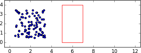
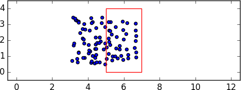
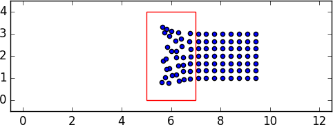
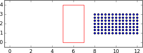
Figure 4: Solution at time $t=0$, $t=2.58$, $t=5.18$ and $t=T=7.75$.

References

- [1] R. Axelrod, The Evolution of Cooperation: Revised Edition. Basic Books, 2006.
- [2] N. Bellomo et al., Active Particles, Volume 1: Advances in Theory, Models, and Applications, ser. Modeling and Simulation in Science, Engineering and Technology. Springer International Publishing, 2017.
- [3] S. Camazine, Self-organization in Biological Systems, ser. Princeton studies in complexity. Princeton University Press, 2003.
- [4] E. Cristiani et al., “Multiscale modeling of pedestrian dynamics,” 2014.
- [5] D. Helbing and R. Calek, Quantitative Sociodynamics: Stochastic Methods and Models of Social Interaction Processes, ser. Theo. and Dec. Lib. B. Springer Neth., 2013.
- [6] M. Jackson, Social and Economic Networks. Princ. Univ. Press, 2010.
- [7] R. Sepulchre, “Consensus on nonlinear spaces,” Ann. rev. in contr., vol. 35, no. 1, pp. 56–64, 2011.
- [8] F. Bullo et al., Distributed Control of Robotic Networks: A Mathematical Approach to Motion Coordination Algorithms, ser. Princ. Ser. in Appl. Math. Princ. Univ. Press, 2009.
- [9] V. Kumar et al., Cooperative Control: Block Island Workshop on Cooperative Control, ser. Lecture Notes in Control and Information Sciences. Springer Berlin Heidelberg, 2004.
- [10] L. Zhiyun et al., “Leader–follower formation via complex Laplacian,” Automatica, vol. 49, no. 6, pp. 1900 – 1906, 2013.
- [11] A. Ferscha and K. Zia, “Lifebelt: Crowd evacuation based on vibro-tactile guidance,” IEEE Pervas. Comp., vol. 9, no. 4, pp. 33–42, 2010.
- [12] P. Luh et al., “Modeling and optimization of building emergency evacuation considering blocking effects on crowd movement,” IEEE Trans. on Autom. Sc. and Eng., vol. 9, no. 4, pp. 687–700, 2012.
- [13] C. Canudas–de–Wit et al., “Graph constrained-CTM observer design for the Grenoble south ring,” IFAC Proceedings Volumes, vol. 45, no. 24, pp. 197–202, 2012.
- [14] A. Hegyi et al., “Specialist: A dynamic speed limit control algorithm based on shock wave theory,” in Intel. Transp. Syst. IEEE, 2008, pp. 827–832.
- [15] M. Duprez et al., “Approximate and exact controllability of the continuity equation with a localized vector field,” Submitted, 2017.
- [16] A. A. Agrachev and Y. Sachkov, Control theory from the geometric viewpoint. Springer Science & Business Media, 2013, vol. 87.
- [17] V. Jurdjevic, Geometric control theory. Cam. uni. press, 1997, vol. 52.
- [18] E. D. Sontag, Mathematical control theory: deterministic finite dimensional systems. Springer Science & Business Media, 2013, vol. 6.
- [19] B. Piccoli et al., “Control to flocking of the kinetic Cucker-Smale model,” J. Math. Anal., vol. 47, no. 6, pp. 4685–4719, 2015.
- [20] M. Caponigro et al., “Mean-field sparse Jurdjevic-Quinn control,” Math. Models Methods Appl. Sci., vol. 27, no. 7, pp. 1223–1253, 2017.
- [21] ——, “Sparse Jurdjevic-Quinn stabilization of dissipative systems,” Automatica J. IFAC, vol. 86, pp. 110–120, 2017.
- [22] M. Duprez et al., “Minimal time problem for crowd models with a localized vector field,” In preparation, 2018.
- [23] C. Villani, Topics in optimal transportation, ser. Graduate Studies in Mathematics. AMS, Providence, RI, 2003, vol. 58.
- [24] J.-M. Coron, Control and nonlinearity, ser. Mathematical Surveys and Monographs. Providence, RI: AMS, 2007, vol. 136.
- [25] M. Krein and D. Milman, “On extreme points of regular convex sets,” Studia Math., vol. 9, pp. 133–138, 1940.