Weight Design of Distributed Approximate Newton Algorithms for Constrained Optimization

Abstract

Motivated by economic dispatch and linearly-constrained resource allocation problems, this paper proposes a novel distributed approx-Newton algorithm that approximates the standard Newton optimization method. A main property of this distributed algorithm is that it only requires agents to exchange constant-size communication messages. The convergence of this algorithm is discussed and rigorously analyzed. In addition, we aim to address the problem of designing communication topologies and weightings that are optimal for second-order methods. To this end, we propose an effective approximation which is loosely based on completing the square to address the NP-hard bilinear optimization involved in the design. Simulations demonstrate that our proposed weight design applied to the distributed approx-Newton algorithm has a superior convergence property compared to existing weighted and distributed first-order gradient descent methods.

I Introduction

Motivation. Networked systems endowed with distributed, multi-agent intelligence are becoming pervasive in modern infrastructure systems such as power networks, traffic networks, and large-scale distribution systems. However, these advancements lead to new challenges in the coordination of the multiple agents operating the network, which are mindful of the network dynamics, availability of partial information, and communication constraints. Distributed algorithms are useful in managing such systems in a manner that elegantly utilizes network resources, which are often (by nature) non-centralized but more scalable. To this end, distributed convex optimization is a rapidly emerging field which seeks to develop such algorithms and understand their properties, e.g. convergence or robustness, from a mathematically rigorous perspective. There are a wide array of techniques that seek to distributively compute the solution to optimization problems. One such problem is economic dispatch, in which a total net load constraint must be satisfied by a set of generators which each have an associated cost of producing electricity. This problem has gained a large amount of recent attention due to the rapid emergence of distributed renewable energy resources, such as wind and solar power and demand response. However, the existing distributed techniques are often limited by speed of convergence. Motivated by this and resource allocation problems in general, we investigate the design of topology weighting strategies that build on the Newton method and lead to improved convergence speeds.

Literature Review. The Newton method for minimizing a real-valued multivariate objective function is well characterized for centralized contexts in [1]. The notion of computing an approximate Newton direction in distributed contexts has gained popularity in recent literature, such as [6] and [4]. In the former work, the authors propose a method which uses the Taylor series expansion for inverting matrices. However, it assumes that each agent keeps an estimate of the entire decision variable, which does not scale well in problems where this variable dimension is equal to the number of agents in the network. Additionally, the optimization is unconstrained, which helps to keep the network decoupled but has a narrower scope in practice. The latter work poses a separable optimization with an equality constraint characterized by the incidence matrix. The proposed approximated Newton method may be not directly applied to networks with constraints that involve the information of all agents. In addition to the aforementioned works, the papers [5, 12, 2] incorporate multi-timescaled dynamics together with a dynamic or online consensus step to speed up the convergence of the agreement subroutine. The aforementioned works only consider uniform edge weight, while sophisticated design of the weighting may improve the convergence. In [11], the Laplacian weight design problem for separable resource allocation is approached from a Distributed Gradient Descent perspective. Solution post-scaling is also presented, which can be found similarly in [7] and [8] for improving the convergence of the Taylor series expression for matrix inverses. In [9], the authors consider edge weight design to minimize the spectrum of Laplacian matrices. However, in the Newton descent framework, the weight design problem formulates as an NP-hard bilinear problem, which is challenging to solve. Overall, the current weight-design techniques that are computable in polynomial time are only mindful of first-order algorithm dynamics. This approach has its challenges, which manifest themselves in a bilinear design problem and more demanding communication requirements, but using second-order information is more heedful of the problem geometry and leads to faster convergence speeds.

Statement of Contributions. In this paper, we propose a novel framework to design a weighted Laplacian matrix that is used in the solution to a multi-agent optimization problem via sparse approximated Newton algorithms. Motivated by economic dispatch, we start by formulating a separable resource allocation problem subject to a global linear constraint, and then derive an equivalent unconstrained form by means of a Laplacian matrix. The Newton steps associated with the unconstrained optimization problem do not inherit the same sparsity as the distributed communication network. To address this issue, we consider approximations based on a Taylor series expansion, where the first few terms inherit certain level of sparsity as prescribed by choice of the Laplacian matrix. We analyze the approximated algorithms and show their (exponential) convergence for any truncation of the series expansion. The effectiveness of the approximation heavily depends on the selection of the weighted Laplacian, which we then set out to optimize. The optimal solution requires solving a NP-hard bilinear optimization problem, which we address by proposing a novel approach which systematically computes an effective solution in polynomial time. A bound on the best-case solution of the original bilinear problem is also given. Furthermore, through a formal statement of the proposed distributed approx-Newton algorithm (or DANA), we find several interesting insights on second-order distributed methods. We compare the results of our design and algorithm to a generic weighting design of Distributed Gradient Descent (DGD) implementations in simulation. Our weighting design shows superior convergence to DGD.

Organization. The rest of the paper is organized as follows. Section II introduces the notations and fundamentals used in this paper. We formulate the optimal resource allocation problem in Section III. In Section IV, we propose a distributed algorithm that approximates the Newton step in solving the optimization. Section V demonstrates the effectiveness of the proposed algorithm. We conclude the paper in Section VI.

II Preliminaries

II-A Notation

Let and ₊ denote the set of real and positive real numbers, respectively, and let ${\mathbb{N}}$ denote the set of natural numbers. For a vector ${x\in^{n}}$, we denote by $x_{i}$ the $i^{\textup{th}}$ entry of $x$. For a matrix ${A\in^{n\times m}}$, we write $A_{i}$ as the $i^{\textup{th}}$ row of $A$ and $A_{ij}$ as the element in the $i^{\textup{th}}$ row and $j^{\textup{th}}$ column of $A$. Discrete time-indexed variables are written as $x^{k}$, where $k$ denotes the current time step. The transpose of a vector or matrix is denoted by $x^{\top}$ and $A^{\top}$, respectively. We use the shorthand notations ${\mathbf{1}_{n}=[1,\dots,1]^{\top}\in^{n}}$, ${\mathbf{0}_{n}=[0,\dots,0]^{\top}\in^{n}}$, and $I_{n}$ to denote the ${n\times n}$ identity matrix. The standard inner product of two vectors $x,y\in^{n}$ is written $\langle x,y\rangle$, and $x\perp y$ indicates $\langle x,y\rangle=0$. For a real-valued function ${f:^{n}\rightarrow}$, the gradient vector of $f$ with respect to $x$ is denoted by ${\nabla_{x}f(x)}$ and the Hessian matrix with respect to $x$ by ${\nabla_{x}^{2}f(x)}$. The positive (semi) definiteness and negative (semi) definiteness of a matrix ${A\in^{n\times n}}$ is indicated by ${A\succ 0}$ and ${A\prec 0}$ (resp. ${A\succeq 0}$ and ${A\preceq 0}$). The set of eigenvalues of a symmetric matrix ${A\in^{n\times n}}$ is ordered as $\lambda_{1}\leq\dots\leq\lambda_{n}$ with associated eigenvectors $v_{1},\dots,v_{n}\in^{n}$. An orthogonal matrix ${T\in^{n\times n}}$ has the property ${T^{\top}T=TT^{\top}=I_{n}}$ and ${T^{\top}=T^{-1}}$. For a finite set $\mathcal{S}$, $|\mathcal{S}|$ is the cardinality of the set. The uniform distribution on the interval $[a,b]$ is indicated by $\mathcal{U}[a,b]$.

II-B Graph Theory

A network of agents is represented by a graph $\mathcal{G}=(\operatorname{\mathcal{N}},\mathcal{E})$, with a node set $\operatorname{\mathcal{N}}=\{1,\dots,n\}$, and edge set $\mathcal{E}\subset\operatorname{\mathcal{N}}\times\operatorname{\mathcal{N}}$. The edge set $\mathcal{E}$ has elements $(i,j)\in\mathcal{E}$ for $j\in\operatorname{\mathcal{N}}_{i}$, where $\operatorname{\mathcal{N}}_{i}\subset\operatorname{\mathcal{N}}$ is the set of out-neighbors of agent $i\in\operatorname{\mathcal{N}}$. The union of out-neighbors to each agent $j\in\operatorname{\mathcal{N}}_{i}$ are the 2-hop neighbors of agent $i$, and denoted by $\operatorname{\mathcal{N}}_{i}^{2}$. More generally, $\operatorname{\mathcal{N}}_{i}^{p}$, or set of $p$-hop neighbors of $i$, is the union of the neighbors of agents in $\operatorname{\mathcal{N}}_{i}^{p-1}$. From this point forward, we consider undirected networks, so ${(i,j)\in\mathcal{E}}$ if and only if ${(j,i)\in\mathcal{E}}$. The graph has an associated weighted Laplacian ${L\in^{n\times n}}$, defined as

$$L_{ij}=\begin{cases}-w_{ij},&j\in\operatorname{\mathcal{N}}_{i},j\neq i,\\ w_{ii},&j=i,\\ 0,&\text{otherwise},\end{cases}$$

with weights $w_{ij}=w_{ji}>0,\forall j\neq i$, and total incident weight $w_{ii}$ on $i\in\operatorname{\mathcal{N}}$, ${w_{ii}=\sum_{j\in\operatorname{\mathcal{N}}_{i}}w_{ij}}$. Evidently, $L$ has an eigenvector ${v_{1}=\mathbf{1}_{n}}$ with an associated eigenvalue ${\lambda_{1}=0}$, and ${L=L^{\top}\succeq 0}$. The graph is connected iif $0$ is a simple eigenvalue, i.e. $0=\lambda_{1}<\lambda_{2}\leq\dots\leq\lambda_{n}$.

A Laplacian $L$ can also be written as a product of its incidence matrix ${E\in\{-1,0,1\}^{|\mathcal{E}|\times n}}$ and a diagonal matrix ${X\in_{+}^{|\mathcal{E}|\times|\mathcal{E}|}}$, whose entries are the weights $w_{ij}$. Each row of $E$ is associated with an edge, which can be alternatively enumerated as $e\in\{1,\dots,|\mathcal{E}|\}$, where the elements $E_{ev}$ are given by

$$E_{ev}=\begin{cases}1,&v=i,\\ -1,&v=j,\\ 0,&\text{otherwise}.\end{cases}$$

Then, $L$ can be written as $L=E^{\top}XE$.

II-C Schur Complement

The following lemma will be used in the sequel.

Lemma 1 ([13]).

(Matrix Definiteness via Schur Complement). Consider a symmetric matrix $M$ of the form

$$M=\begin{bmatrix}A&B\\ B^{\top}&C\end{bmatrix}.$$

If $C$ is invertible, then the following properties hold:
(1) $M\succ 0$ if and only if $C\succ 0$ and $A-BC^{-1}B^{\top}\succ 0$.
(2) If $C\succ 0$, then $M\succeq 0$ if and only if $A-BC^{-1}B^{\top}\succeq 0$.

II-D Taylor Series Expansion for Matrix Inverses

A full-rank matrix $A\in^{n\times n}$ has a matrix inverse, $A^{-1}$, which is characterized by the relation $AA^{-1}=I_{n}$. In general, it is not straightforward to compute this inverse via a distributed algorithm. However, if the eigenvalues of $A$ satisfy $|1-\lambda_{i}(A)|<1,\forall\,i\in\mathcal{N}$, then we can employ the Taylor expansion to compute its inverse as follows:

$$A^{-1}=\sum_{p=0}^{\infty}(I_{n}-A)^{p}.$$

Note that, if the sparsity structure of $A$ represents a network topology, then traditional matrix inversion techniques such as Gauss-Jordan elimination still necessitate all-to-all communication. However, agents can communicate and compute locally to obtain each term in the previous expansion. It can be seen via the diagonalization of $I_{n}-A$ that the terms of the sum become small as $p$ increases due to the assumption on the eigenvalues of $A$. The convergence of these terms is exponential and limited by the slowest converging mode, i.e. $\max{|1-\lambda_{i}(A)|}$.

We can compute an approximation of $A^{-1}$, denoted by $\widetilde{A^{-1}_{q}}$, in finite steps by computing and summing the terms up to the $q^{\textup{th}}$ power. We refer to this approximation as a q-approximation of $A^{-1}$.

III Problem Statement

Motivated by the economic dispatch problem, in this section, we pose the separable resource allocation that we aim to solve distributively. We reformulate it as an unconstrained optimization problem whose decision variable is in the span of the graph Laplacian, and motivate the characterization of a second-order Newton-inspired method.

Consider a group $\operatorname{\mathcal{N}}$ of agents or nodes, indexed by $i\in\operatorname{\mathcal{N}}$, each associated with a local convex cost function $f_{i}:\rightarrow$, $i\in\operatorname{\mathcal{N}}$. These agents can be thought of as generators in an electricity market, where each function argument, $x_{i}\in$, $i\in\operatorname{\mathcal{N}}$, represents the power in megawatts that agent $i$ produces at a cost characterized by $f_{i}$. The economic dispatch problem aims to satisfy a global load-balancing constraint $\sum_{i=1}^{n}x_{i}=d$ for minimal global cost $f:^{n}\rightarrow$, where $d$ is the total load consumption in megawatts. We relax the full problem by excluding the box constraints on the states $x_{i}$. Then, the relaxed economic dispatch optimization problem we are interested in solving is stated as:

$${\mathcal{P}}1:\quad \underset{x}{\min}\quad f(x)=\sum_{i=1}^{n}f_{i}(x_{i})$$ (1)

s.t. $$\sum_{i=1}^{n}x_{i}=d.$$ (2)

Excluding the box constraints has the effect of allowing some states to be negative, which physically could addressed via curtailment of some baseline loads. For simplicity, we do not consider these constraints here; addressing this question via quadratic loss functions is the subject of current work. Distributed optimization algorithms based on a gradient descent approach are available to solve ${\mathcal{P}}1$ [14]. However, by only taking into account first-order information of the cost functions, these methods tend to be inherently slow. As for a Newton (second-order) method, the computation of the descent direction is not distributed. To see this, recall the unconstrainted Newton step defined as ${\Delta x_{\textup{nt}}:=-\nabla^{2}f(x)^{-1}\nabla f(x)}$, see e.g. [1]. In this context, the equality constraint can be eliminated by imposing ${x_{n}=d-\sum_{i=1}^{n-1}x_{i}}$. Then, (1) becomes ${f(x)=\sum_{i=1}^{n-1}f_{i}(x_{i})+f_{n}(d-\sum_{i=1}^{n-1}x_{i})}$. In general, the resulting Hessian $\nabla^{2}_{x}f(x)$ is fully populated and its inverse requires all-to-all communication among agents in order to compute the second-order descent direction.

Instead, we eliminate (2) by introducing a network topology as encoded by a Laplacian matrix $L$ associated with a connected graph $G$, and an initial condition $x^{0}\in^{n}$, with the following assumptions.

Assumption 1.

(Symmetric Laplacian matrix). The weighted graph characterized by $L$ is undirected and connected, i.e. $L=L^{\top}$ and $0$ is a simple eigenvalue of $L$.

Assumption 2.

(Feasible initial condition). The initial state $x^{0}$ is a feasible point of ${\mathcal{P}}1$, i.e.

$$\sum_{i=1}^{n}x_{i}^{0}=d.$$

The objective and constraint  (1)–(2) can now be restated as the following equivalent problem:

$${\mathcal{P}}2:\quad \underset{z}{\min}\quad f(x^{0}+Lz)=\sum_{i=1}^{n}\textit{f}_{i}(x_{i}^{0}+L_{i}z).$$

Using the property that $\mathbf{1}_{n}$ is an eigenvector associated with $\lambda_{1}=0$ we have that $\mathbf{1}_{n}^{\top}(x^{0}+Lz)=d$ for any $z\in^{n}$. Then, the solution to ${\mathcal{P}}2$ is a feasible and optimal solution to ${\mathcal{P}}1$. An analogous formulation of equality constrained Newton descent for centralized solvers is given in [1]; in our distributed framework, the row space of the Laplacian is a useful property to address (2).

We aim to leverage the freedom given by the elements of $L$ in order to compute an approximate Newton direction to ${\mathcal{P}}2$, denoted by $\tilde{z}_{\textup{nt}}$. In every iteration $k$, the approximated Newton step $\tilde{z}_{\textup{nt}}$ is used to update $x^{k}$ by the following

$$x^{k+1}=x^{k}+\alpha L\tilde{z}_{\textup{nt}},$$ (3)

where $\alpha>0$ is a step size. There is agent-to-agent communication and local computations embedded in this informal statement, which will be described and restated formally in the following section.

IV Main Results

In this section, we characterize an approximate Newton step that can be computed distributively to solve problem ${\mathcal{P}}1$. We then pose the weight-design problem and develop an approximation which enables a solution to be computed in polynomial time. Next, we provide a method for estimating the best-case scenario of the solution to the NP-hard problem. We then formally state the distributed approx-Newton algorithm and rigorously analyze its convergence properties.

IV-A Characterization of the Approximate Newton Step

First, note that the Hessian of (1), $H:=\nabla_{x}^{2}f(x)$, is diagonal. In addition, we adopt the following assumption.

Assumption 3.

(Quadratic cost functions). The local costs can be written in the form $f_{i}(x_{i})=\dfrac{1}{2}a_{i}x_{i}^{2}+b_{i}x_{i}$ with $a_{i}\in_{+},b_{i}\in$. In light of this, given $\delta=\min(a_{i}),\gamma=\max(a_{i})$, then

$$0\prec\delta I_{n}\preceq\nabla_{x}^{2}f(x)=H\preceq\gamma I_{n}.$$

This ensures $H=\operatorname{diag}(a_{i})$ is constant, which is necessary to construct the notion of an optimal $L$. In fact, this is a widely accepted model for generator costs, and the assumption is common in the literature for addressing economic dispatch. We use $b\in^{n}$ to refer to the vector of linear coefficients.

The Hessian of the unconstrained problem with respect to $z$ can then be computed as $\nabla_{z}^{2}f(x_{0}+Lz)=LHL$. We would like to find an analogous Newton step in $z$ to solve ${\mathcal{P}}2$, but clearly $LHL$ is non-invertible due to the smallest eigenvalue of $L$ fixed at zero, a manifestation of the equality constraint in the original problem ${\mathcal{P}}1$.

To reconcile with this, we change the coordinates of $z$ by the orthogonal matrix $T$ given as

$$T=\begin{bmatrix}n-1+\sqrt{n}&-1&\cdots&-1&\dfrac{1}{\sqrt{n}}\\ -1&\ddots&\cdots&\vdots&\\ \vdots&&\ddots&-1&\vdots\\ -1&\cdots&-1&n-1+\sqrt{n}&\\ -1-\sqrt{n}&\cdots&\cdots&-1-\sqrt{n}&\dfrac{1}{\sqrt{n}}\end{bmatrix}\text{diag}(\begin{bmatrix}\rho\\ 1\end{bmatrix}),$$

where $\rho=\sqrt{n(n+1+2\sqrt{n})}^{-1}\mathbf{1}_{n-1}$. This transformation leaves the last column as a constant multiple of the all ones vector. The new coordinates allow us to rewrite $Lz$ with a reduced order variable $\hat{z}\in^{n-1}$. More specifically, $Lz=LTJ^{\top}\hat{z}$, where $J=\begin{bmatrix}I_{n-1}&\mathbf{0}_{n-1}\end{bmatrix}$. We then rewrite $f$ by substituting $z$ by $\hat{z}$

$$f(x^{k}+Lz) =\dfrac{1}{2}z^{\top}LHLz+\dfrac{1}{2}x^{k\top}Hx^{k}+z^{\top}LHx^{k}$$

$$+z^{\top}Lb+x^{k\top}b$$

$$=\dfrac{1}{2}\hat{z}^{\top}JT^{\top}LHLTJ^{\top}\hat{z}+\dfrac{1}{2}x^{k\top}Hx^{k}$$

$$+\hat{z}^{\top}JT^{\top}(Lb+LHx^{k})+x^{k\top}b.$$

Taking the gradient and Hessian with respect to $\hat{z}$ in this expression gives

$$\nabla_{\hat{z}}f(x^{k}+Lz) =JT^{\top}LHLTJ^{\top}\hat{z}+JT^{\top}(Lb+LHx^{k})$$

$$\nabla_{\hat{z}}^{2}f(x^{k}+Lz) =JT^{\top}LHLTJ^{\top}.$$

Notice that the zero eigenvalue of $\nabla_{z}^{2}f$ is eliminated by the projection. The Newton step associated with $\hat{z}$ is then well defined as ${\hat{z}_{\textup{nt}}=-(\nabla_{\hat{z}}^{2}f)^{-1}\nabla_{\hat{z}}f}$. For brevity, we define $M=JT^{\top}LHLTJ^{\top}$ and $v(x^{k})=Lb+LHx^{k}$. The Newton step in $\hat{z}$ is rewritten as ${\hat{z}_{\textup{nt}}=-M^{-1}(M\hat{z}+JT^{\top}v(x^{k}))}$ which, when evaluated at $z=0$, reduces to $\hat{z}_{\textup{nt}}=-M^{-1}JT^{\top}v(x^{k})$.

Now, consider a $q$-approximation of $M^{-1}$ given by $\widetilde{M_{q}^{-1}}=\sum_{p=0}^{q}(I_{n-1}-M)^{p}$. We can then approximate $\hat{z}_{\textup{nt}}$ as $-\widetilde{M_{q}^{-1}}JT^{\top}v(x^{k})$. Returning to the original coordinates:

$$Lz_{\textup{nt}}\approx L\tilde{z}_{\textup{nt}}=-LTJ^{\top}\sum_{p=0}^{q}(I_{n-1}-M)^{p}JT^{\top}v(x^{k}).$$

With the property that $LTJ^{\top}JT^{\top}L=LL$, we can rewrite $L\tilde{z}_{\textup{nt}}$ as

$$L\tilde{z}_{\textup{nt}}=-L\sum_{p=0}^{q}(I_{n}-LHL)^{p}(Lb+LHx^{k}).$$ (4)

The series $L(I_{n}-LHL)^{p}$ converges with $p\rightarrow\infty$ if the following assumption holds.

Assumption 4.

(Convergent eigenvalues). The smallest $n-1$ eigenvalues of $(I_{n}-LHL)$ are contained in the unit ball, i.e. $\exists\ \varepsilon<1$ such that

$$-\varepsilon I_{n-1}\preceq(I_{n-1}-M)\preceq\varepsilon I_{n-1}.$$

In the following section, we address Assumption 4 by minimizing $\varepsilon$ via weight design of the Laplacian. By doing this, we aim to obtain a good approximation of $M^{-1}$ from the Taylor expansion with small $q$.

IV-B Weight Design of the Laplacian

Our approach returns to the intuition on the rate of convergence of the $q$-approximation of $M^{-1}$. We design a weighting scheme for a communication topology characterized by $L$ which lends itself to a scalable, fast approximation of $z_{\textup{nt}}$. To do this, we aim to minimize $\max|1-\lambda_{i}(M)|$, and pose this problem as

$${\mathcal{P}}3: \underset{\varepsilon,L}{\text{min}} \varepsilon$$

s.t. $$-\varepsilon I_{n-1}\preceq I_{n-1}-M\preceq\varepsilon I_{n-1},$$

$$L\mathbf{1}_{n}=\mathbf{0}_{n},\ L\succeq 0,$$

$$L_{ij}=0,\,j\notin\operatorname{\mathcal{N}}_{i}.$$

There is one nonconvexity in this problem given by the right side of the matrix inequality, which is bilinear in $L$. If we ignore the sparsity constraint on $L$, it is possible to treat the constraint as an LMI in $M$, obtain an exact solution, and then perform some eigendecomposition on $M$ and compute a nonsparse solution in $L$. However, implementing this solution would be non-distributed. There are path-following techniques available to solve bilinear problems of this form [3], but simulation results do not produce a satisfactory solution via this method. For this reason, we develop a convex approximation of ${\mathcal{P}}3$.

Consider $\varepsilon_{-}$ and $\varepsilon_{+}$ corresponding to the left-hand (convex) and right-hand (nonconvex) matrix inequalities, respectively. To handle $-\varepsilon_{-}I_{n-1}\preceq I_{n-1}-M$, we write $L$ as a weighted product of its incidence matrix, $L=E^{\top}XE$. Applying Lemma 1 makes the constraint become

$$\begin{bmatrix}(\varepsilon_{-}+1)I_{n-1}&JT^{\top}E^{\top}XE\\ E^{\top}XETJ^{\top}&H^{-1}\end{bmatrix}\succeq 0.$$ (5)

As for the right-hand side $I_{n-1}-M\preceq\varepsilon_{+}I_{n-1}$, consider the approximation $LHL\approx\left(\dfrac{\sqrt{H}L+L\sqrt{H}}{2}\right)^{2}$. Substitute this in $M$ to get

$$\dfrac{1}{4}JT^{\top}(\sqrt{H}L+L\sqrt{H})^{2}TJ^{\top}\succeq(1-\varepsilon_{+})I_{n-1}$$

$$\dfrac{1}{2}JT^{\top}(\sqrt{H}L+L\sqrt{H})TJ^{\top}\succeq\sqrt{(1-\varepsilon_{+})}I_{n-1}$$

$$\dfrac{1}{2}JT^{\top}(\sqrt{H}L+L\sqrt{H})TJ^{\top}\succeq(1-\dfrac{\varepsilon_{+}}{2}+\dfrac{\varepsilon_{+}^{2}}{8}+O(\varepsilon_{+}^{3}))I_{n-1},$$

where the second line uses the property that $A^{2}\succeq(1-\varepsilon_{+})I_{n-1}\succeq 0\Leftrightarrow A\succeq\sqrt{1-\varepsilon_{+}}I_{n-1}\succeq 0$ [10], and that $TJ^{\top}JT^{\top}=I_{n}-\mathbf{1}_{n}\mathbf{1}_{n}^{\top}/n$ is idempotent. The third line expresses the right-hand side as a Taylor expansion about $\varepsilon_{+}=0$. Neglecting the higher order terms in $\varepsilon_{+}$, and applying Lemma 1 gives

$$\begin{bmatrix}\bullet&\dfrac{1}{\sqrt{8}}\varepsilon_{+}I_{n-1}\\ \dfrac{1}{\sqrt{8}}\varepsilon_{+}I_{n-1}&I_{n-1}\end{bmatrix}\succeq 0,$$ (6)

where ${\bullet=\dfrac{1}{2}JT^{\top}(\sqrt{H}L+L\sqrt{H})TJ^{\top}}-{(1-\dfrac{1}{2}\varepsilon_{+})I_{n-1}}$.

Returning to ${\mathcal{P}}3$, note that the latter three constraints are addressed by writing $L=E^{\top}XE$. Then, the approximate reformulation of ${\mathcal{P}}3$ can be written as

$${\mathcal{P}}4: \underset{\varepsilon_{-},\varepsilon_{+},X}{\text{min}} \max(\varepsilon_{-},\varepsilon_{+})$$

s.t. $$\varepsilon_{-}\geq 0,\varepsilon_{+}\geq 0,$$

$$X\succeq 0,\eqref{ineq:convex_constraint},\eqref{ineq:nonconvex_constraint}.$$

This is a convex problem in $X$ and solvable in polynomial time. To improve the solution, we perform some post-scaling. Take $L^{\star}_{0}=E^{\top}X_{0}^{\star}E$, where $X_{0}^{\star}$ is the solution to ${\mathcal{P}}4$, and ${M^{\star}_{0}=JT^{\top}L^{\star}_{0}HL^{\star}_{0}TJ^{\top}}\succ 0$. Then, consider

$$\beta=\sqrt{\dfrac{2}{\lambda_{1}(M^{\star}_{0})+\lambda_{n-1}(M^{\star}_{0})}}$$

and take $L^{\star}=\beta L^{\star}_{0}$. This shifts the eigenvalues of $M^{\star}_{0}$ to $M^{\star}$ (defined similarly via $L^{\star}$) such that $1-\lambda_{1}(M^{\star})=-(1-\lambda_{n-1}(M^{\star}))$, which shrinks $\max(|1-\lambda_{i}(M^{\star})|)$. We refer to this metric as $\varepsilon_{L^{\star}}:=\max(|1-\lambda_{i}(M^{\star})|)$. In fact, it can be verified that this post-scaling guarantees $\varepsilon_{L^{\star}}$ satisfies Assumption 4. Then, the solution to ${\mathcal{P}}4$ followed by a post scaling by $\beta$ given by $L^{\star}$ is an approximation of the solution to the nonconvex problem ${\mathcal{P}}3$ with the sparsity structure preserved.

IV-C A Bound on Performance

It should be unsurprising that, given a sparsity structure for the network, even the globally optimal solution to ${\mathcal{P}}3$ will typically produce a nonzero $\varepsilon$. We are then motivated to find a “best-case scenario” for our solution given the structure of the network. The approach for this is straightforward: instead of solving ${\mathcal{P}}3$ for $L$, we solve it for some $A$ where $A$ has the sparsity structure of $LHL$, i.e. the two-hop neighbor structure of the network. Define $M_{A}:=JT^{\top}ATJ^{\top}$. This problem is stated as:

$${\mathcal{P}}5: \underset{\varepsilon,A}{\text{min}} \varepsilon$$

s.t. $$-\varepsilon I_{n-1}\preceq I_{n-1}-M_{A}\preceq\varepsilon I_{n-1},$$

$$A\mathbf{1}_{n}=\mathbf{0}_{n},\ A\succeq 0,$$

$$A_{ij}=0,j\notin\operatorname{\mathcal{N}}^{2}_{i}.$$

This problem is convex in $A$ and produces a solution $\varepsilon_{A}$, which serves as a lower bound for the solution to ${\mathcal{P}}3$. Of course, there may not exist an $L$ with the desired sparsity such that $LHL=A$, $\forall A$ in the feasibility set of ${\mathcal{P}}5$. This is what makes ${\mathcal{P}}3$ difficult to solve, but it gives us some notion for how effective the post-scaled solution to ${\mathcal{P}}4$ is in the following sense: $\varepsilon_{L^{\star}}-\varepsilon_{A}$ indicates how close $\varepsilon_{L^{\star}}$ is to the lower bound of the global optimum of ${\mathcal{P}}3$.

IV-D The distributed approx-Newton Algorithm

We now have the tools that we need to introduce the DANA, or the distributed approx-Newton algorithm.

Algorithm 1 distributed approx-Newton

1:$L_{j},a_{j},b_{j}$ for $j\in\{i\}\cup\operatorname{\mathcal{N}}_{i}$ and communication with nodes $j\in\operatorname{\mathcal{N}}_{i}\cup\operatorname{\mathcal{N}}_{i}^{2}$

2:procedure Newton($x^{0},L,H,b,q$)

3:     Initialize $x^{0}$

4:     for $k=0,1,\dots$ do

5:         for all $i$ do

6:              Acquire $x_{j}^{k}$ for $j\in\operatorname{\mathcal{N}}_{i}$

7:              $y_{i}\leftarrow L_{i}b+(LH)_{i}x^{k}$

8:              $z_{i}\leftarrow-y_{i}$

9:         end for

10:         for $p=1,\dots,q$ do

11:              for all $i$ do

12:                  Acquire $y_{j}$ for $j\in\operatorname{\mathcal{N}}_{i}^{2}$

13:                  $w_{i}=(I_{n}-LHL)_{i}y$

14:              end for

15:              $y\leftarrow w$

16:              $z\leftarrow z-y$

17:         end for

18:         for all $i$ do

19:              Acquire $z_{j}$ for $j\in\operatorname{\mathcal{N}}_{i}$

20:              Compute $x_{i}^{k+1}=x_{i}^{k}+\alpha L_{i}z$

21:         end for

22:     end for

23:     return $x$

24:end procedure

The algorithm is constructed directly from (3) and (4). The right-hand factor of (4) is computed first in the loop starting on line 5. Then, each additional term of the sum is computed recursively in the loop starting on line 10, where $w$ is used as an intermediate variable. The outer loop of the algorithm is performed starting on line 18. The process then repeats for a desired number of time steps $k$. If $q$ is increased, it requires additional inner-loops and two-hop communications, but the step approximation will be more accurate.

It may come as a surprise that the effect of increasing the inner loop parameter $q$ by $1$ is algebraically equivalent to taking an additional outer loop step at $q=0$. To see this, consider $\hat{x}^{k+1}=x^{k}+L\tilde{z}_{\textup{nt}}^{+}=x^{k}+L\left(\tilde{z}_{\textup{nt}}-(I-LHL)^{q+1}(Lb+LHx^{k})\right)$. The polynomial part of the additional term can be quickly expanded with the coefficients given by the $(q+1)^{\textup{th}}$ row of Pascal’s triangle, which then gets multiplied from the right by $Lb$ and $LHx^{k}$. Compare this to the two-step iteration: $x^{k+1}=x^{k}+L\tilde{z}_{\textup{nt}}$ followed by $x^{k+2}=x^{k+1}-L(Lb+LHx^{k+1})$, i.e. two outer loops with the second loop using $q=0$. It is the case that $\hat{x}^{k+1}=x^{k+2}$ and these implementations give an equivalent result.

This has some interesting consequences. Applying this “loop conversion” notion recursively, it follows that an implementation using some $q_{a}$ inner loop parameter with $k_{a}$ outer loops can be converted to an equivalent implementation with $k_{0}=(q_{a}+1)k_{a}$ outer loops and $q_{0}=0$ inner loop parameter. Then, this can be converted again to some $q_{b}$ implementation with $k_{b}=k_{0}/(q_{b}+1)$ outer loops. If $q_{b}+1$ is not a divisor of $k_{0}$, the “remainder” can be made up with an additional outer loop using an appropriate $q_{c}<q_{b}$ parameter.

A concise summary can be made with the following relation: if $k_{a},q_{a},k_{b}$ and $q_{b}$ are such that

$$k_{a}(q_{a}+1)=k_{b}(q_{b}+1)$$ (7)

holds, then implementing the DANA from the same $x^{0}$ will result in $x^{k_{a}}=x^{k_{b}}$. With this in mind, if direct two-hop communications are not available, message passing is required and it is less desirable to implement inner-loop iterations when communications are failing or lossy. Future work will be devoted to evaluate the performance of the alternative approaches with various $q$ under the presence of message failures.

IV-E Convergence Analysis

This section establishes convergence properties of the distributed approx-Newton algorithm for problems of the form ${\mathcal{P}}1$.

Theorem 1.

(Convergence of DANA). If Assumption 1, on the bidirectional connected graph, Assumption 2, on the feasibility of the initial condition, Assumption 3, on quadratic cost functions, and Assumption 4, on convergent eigenvalues, hold, then the optimal solution $x^{\star}$ of ${\mathcal{P}}1$ is a unique globally exponentially stable point under the dynamics of the distributed approx-Newton algorithm for any $q\in{\mathbb{N}}$.

Proof.

For uniqueness, consider the KKT condition which gives the linear relation:

$$\begin{pmatrix}H&\mathbf{1}_{n}\\ \mathbf{1}^{\top}_{n}&0\end{pmatrix}\begin{pmatrix}x^{\star}\\ \lambda^{\star}\end{pmatrix}=\begin{pmatrix}-b\\ d\end{pmatrix},$$

where $\lambda^{\star}$ is the optimal Lagrange multiplier. It is easy to verify that the left-hand side matrix is nonsingular, which gives a unique solution $x^{\star}$.

We establish convergence via a discrete-time Lyapunov function and assuming a unit step size without loss of generality. Consider the symmetric matrix $L^{\dagger}$ characterized by $LL^{\dagger}=I_{n}-\mathbf{1}_{n}\mathbf{1}_{n}^{\top}/n,$ $\operatorname{null}(L^{\dagger})=\operatorname{span}(\mathbf{1}_{n})$. Let ${V(x^{k})=(x^{k}-x^{\star})^{\top}L^{\dagger}L^{\dagger}(x^{k}-x^{\star})}$, which is well defined for any $x\in^{n}$, $\sum_{i}x_{i}=d$. The dynamics of DANA are given by $x^{k+1}=x^{k}+L\tilde{z}_{\textup{nt}}$, where $\tilde{z}_{\textup{nt}}=-\sum_{p=0}^{q}(I_{n}-LHL)^{p}v(x^{k})$, where recall that $v(x^{k})=Lb+LHx^{k}$. We have $V(x^{k})>0,$ $\ \forall x^{k}$ such that $\sum_{i}x_{i}^{k}=d,x^{k}\neq x^{\star}$ (which follows from $(x^{k}-x^{\star})\notin\operatorname{null}(L^{\dagger})$), $V$ is radially unbounded over the space where $\sum_{i}x_{i}=d$, and $V(x^{\star})=0$. Hence, $V$ is a Lyapunov function candidate. We aim to show ${V(x^{k+1})-V(x^{k})<0}$, for any $q\in{\mathbb{N}}$ and $k\geq 0$, where

$$V(x^{k+1})-V(x^{k})=V(x^{k}+L\tilde{z}_{\textup{nt}})-V(x^{k})$$ (8)

$$=2\tilde{z}_{\textup{nt}}^{\top}LL^{\dagger}L^{\dagger}(x^{k}-x^{\star})+\tilde{z}_{\textup{nt}}^{\top}(I_{n}-\mathbf{1}_{n}\mathbf{1}_{n}^{\top}/n)\tilde{z}_{\textup{nt}}.$$

Since we consider optimization with quadratic cost functions, an exact Newton step solves the problem in one step. In other words, $x^{k}-x^{\star}=-Lz_{\textup{nt}}=L\sum_{p=0}^{\infty}(I_{n}-LHL)^{p}v(x^{k})$ holds. Next, define $A_{1}:=\sum_{p=0}^{q}(I_{n}-LHL)^{p}$ and $A_{2}:=\sum_{p=0}^{\infty}(I_{n}-LHL)^{p}$, for brevity. Note that $A_{2}$ is not a convergent series expansion due to the non-converging mode, but the argument given in Section IV-A as to “canceling” this mode via multiplication by $L$ is applicable. To see that $A_{1}\succ 0$ for $q$ odd, we write $A_{1}=\sum_{l=0}^{(q-1)/2}(2I_{n}-LHL)(I_{n}-LHL)^{2l}$. Note that each term in $A_{1}$ is symmetric and positive definite due to $(2I_{n}-LHL)\succ 0,(I_{n}-LHL)^{2l}\succ 0$, and the product being symmetric. For the case of $q$ even, the last term is $(I_{n}-LHL)^{q}\succ 0$.

Finally, note that $LL^{\dagger}=LL^{\dagger}L^{\dagger}L=(I_{n}-\mathbf{1}_{n}\mathbf{1}_{n}^{\top}/n)$ is idempotent. Returning to the matter at hand, substituting in (8) gives

$$V(x^{k+1})-V(x^{k}) =-2v(x^{k})^{\top}A_{1}(I_{n}-\mathbf{1}_{n}\mathbf{1}_{n}^{\top}/n)A_{2}v(x^{k})$$ (9)

$$+v(x^{k})^{\top}A_{1}(I_{n}-\mathbf{1}_{n}\mathbf{1}_{n}^{\top}/n)A_{1}v(x^{k}).$$

We have that $v(x^{k})\perp\mathbf{1}_{n}$, so showing the negativity of (9) is equivalent to showing

$$2A_{1}(I_{n}-\mathbf{1}_{n}\mathbf{1}_{n}^{\top}/n)A_{2}-A_{1}(I_{n}-\mathbf{1}_{n}\mathbf{1}_{n}^{\top}/n)A_{1}\\ \succeq c(I_{n}-\mathbf{1}_{n}\mathbf{1}_{n}^{\top}/n),$$ (10)

for some $c>0$. To show this, rewrite $A_{2}=\sum_{l=0}^{\infty}(I_{n}-LHL)^{l(q+1)}A_{1}$. Then, (10) can be written as

$$A_{1}(I_{n}-\mathbf{1}_{n}\mathbf{1}_{n}^{\top}/n)\left(\sum_{l=0}^{\infty}\Big{[}2(I_{n}-LHL)^{l(q+1)}\Big{]}-I_{n}\right)A_{1}\\ \succeq c(I_{n}-\mathbf{1}_{n}\mathbf{1}_{n}^{\top}/n).$$ (11)

For $q$ odd, it is straightforward to see this holds. The $-I_{n}$ cancels with an $l=0$ term and the remaining terms are raised to even powers. Therefore the left-hand side is positive definite and such $c$ can be found. For $q$ even, we use the bound

$$\bullet \succeq A_{1}(I_{n}-\mathbf{1}_{n}\mathbf{1}_{n}^{\top}/n)\left(\sum_{l=0}^{\infty}\left[2(-\varepsilon)^{l(q+1)}\right]-1\right)A_{1}$$ (12)

$$=A_{1}(I_{n}-\mathbf{1}_{n}\mathbf{1}_{n}^{\top}/n)\left(\dfrac{2}{1+\varepsilon^{q+1}}-1\right)A_{1}$$

$$\succeq c(I_{n}-\mathbf{1}_{n}\mathbf{1}_{n}^{\top}/n),$$

where $\bullet$ is the top line of (11). To see this, write $I_{n}-LHL=QDQ^{-1}$ as its Jordan decomposition, where $D$ is a matrix consisting of the Jordan blocks of $I_{n}-LHL$ whose diagonal entries are given by the vector $\operatorname{diag}(D)=(1,\eta_{1},\dots\eta_{n-1})$ where $\eta_{i}\in[-\varepsilon,\varepsilon],$ for $i=1,\dots,n-1$. Then, $(I_{n}-LHL)^{l(q+1)}=QD^{l(q+1)}Q^{-1}$ with $D^{l(q+1)}$ upper triangular. The smallest diagonal entry of $\sum_{l=0}^{\infty}D^{l(q+1)}$ is bounded from below by $\sum_{l=0}^{\infty}(-\varepsilon)^{l(q+1)}$. Finally, we arrive at the relation

$$(I_{n}-\mathbf{1}\mathbf{1}_{n}^{\top}/n)\sum_{l=0}^{\infty}2QD^{l(q+1)}Q^{-1}\\ \succeq(I_{n}-\mathbf{1}\mathbf{1}_{n}^{\top}/n)\sum_{l=0}^{\infty}2(-\varepsilon)^{l(q+1)},$$

which gives the bound in (12). From Assumption 4 we have $\varepsilon\in[0,1)$. This verifies (11) ($q$ odd) or (12) ($q$ even) hold for some $c>0$. This is sufficient to show $x^{\star}$ is a globally asymptotically stable point under the dynamics of distributed approx-Newton algorithm.

For exponential convergence, we are interested in showing $V(x^{k+1})\leq(1-\hat{c})V(x^{k})$ for some $\hat{c}\in(0,1)$ that is independent of $k$. Consider the $q=0$ case without loss of generality. Note that $v(x^{\star})=0$, implying $v(x^{k})=v(x^{k})-v(x^{\star})=LH(x^{k}-x^{\star})$. Then, substituting in (9) and using the $c$ characterized by (11)–(12) gives

$$V(x^{k+1}) \leq V(x^{k})-c(v(x^{k})^{\top}LL^{\dagger}L^{\dagger}Lv(x^{k}))$$ (13)

$$=V(x^{k})-c(x^{k}-x^{\star})^{\top}HL^{2}L^{\dagger 2}L^{2}H(x^{k}-x^{\star})$$

$$\leq(1-\hat{c})V(x^{k}),$$

where $\hat{c}\in(0,1)$ is a function of $c,L$, and $H$, and $\hat{c}>0$ due to $v(x^{k})\perp\operatorname{null}{(L)}$. This shows the Lyapunov function exponentially decays at a rate characterized by $\hat{c}$. ∎

V Simulations and Discussion

In this section, we implement our weight design and verify the convergence of the distributed approx-Newton algorithm for different $q\geq 0$, and compare their speed of convergence in terms of the number of outer loops $k$ employed. Returning to the economic dispatch motivation, we consider a network with $n=50$ generators and $|\mathcal{E}|=150$ randomly generated bidirectional communication links between generators. The local computations required of each generator are simple vector operations whose dimension scales linearly with the network size, which can be implemented on a microprocessor. The graph topology is plotted in Figure 1. The cost coefficients are generated as $a_{i}\in\mathcal{U}\left[0.8,1.2\right],$ $b_{i}\in\mathcal{U}\left[0,1\right],$ and power requirement is taken to be $d=50$MW. We compare to Distributed Gradient Descent (DGD) with unit step size and two weightings on $L$. The first is “unweighted”, in the sense that $L$ is taken to be the degree matrix minus the adjacency matrix of the graph, followed by the post-scaling described in Section IV-B to guarantee convergence. The second weighting on $L$ for DGD is proposed in [11]. The results are given in Figure 2, which shows linear convergence to the optimal value as the number of iterations increases, with fewer iterations needed for larger $q$. We note a substantially improved outer-loop convergence over the DGD methods, even for the $q=0$ case which utilizes an equal number of agent-to-agent communications as DGD.

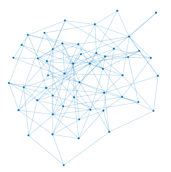
Figure 1: Communication topology used for comparisons of distributed approx-Newton and DGD.

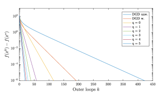
Figure 2: Convergence of distributed approx-Newton for varying $q$ compared to unweighted and weight-designed DGD.

On the weighting design side, consider the following metrics. The solution to ${\mathcal{P}}4$ followed by the post-scaling by $\beta$ gives $\varepsilon_{L^{\star}}:=\max(|1-\lambda_{i}(M^{\star})|)$; this metric represents the convergence speed of distributed approx-Newton when applying our proposed weight design of $L$. Using the same topology $(\operatorname{\mathcal{N}},\mathcal{E})$, the solution to ${\mathcal{P}}5$ gives the metric $\varepsilon_{A}$. Note that $\varepsilon_{A}$ is a best-case estimate of the weight design problem, which cannot be implemented in practice, while $\varepsilon_{L^{\star}}$ is the metric for which we can compute an $L^{\star}$. The objective of each problem is to minimize the associated $\varepsilon$; to this end, we aim to characterize the relationship between network parameters and these metrics. We ran 100 trials on each of 16 test cases which encapsulate a variety of parameter cases: two cases for the cost coefficients, a tight distribution $a_{i}\in\mathcal{U}\left[0.8,1.2\right]$ and a wide distribution $a_{i}\in\mathcal{U}\left[0.2,5\right]$. For topologies, we randomly generated connected graphs with network size $n\in\{10,20,30,40,50\}$, a linearly scaled number of edges $|\mathcal{E}|=3n$, and a quadratically scaled number of edges $|\mathcal{E}|=0.16n^{2}$ for the $n\in\{30,40,50\}$ cases. The linearly scaled connectivity case corresponds to keeping the average degree of a node constant for increasing network sizes, while the quadratically scaled case roughly preserves the proportion of connected edges to total possible edges, which is a quadratic function of $n$ and equal to $n(n-1)/2$ for an undirected network. The results are depicted in Table I. This gives the mean $\mu$ and standard deviation $\sigma$ of the distributions for performance $\varepsilon_{L^{\star}}$ and performance gap $\varepsilon_{L^{\star}}-\varepsilon_{A}$.

Table I: Laplacian Design

$a_{i}\in\mathcal{U}\left[0.8,1.2\right]$ $b_{i}\in\mathcal{U}\left[0,1\right]$	$\mu(\varepsilon_{L^{\star}})$	$\sigma(\varepsilon_{L^{\star}})$	$\mu(\varepsilon_{L^{\star}}-\varepsilon_{A})$	$\sigma(\varepsilon_{L^{\star}}-\varepsilon_{A})$
$n=10$ $|\mathcal{E}|=30$	0.6343	0.0599	0.2767	0.0186
$n=20$ $|\mathcal{E}|=60$	0.8655	0.0383	0.2879	0.0217
$n=30$ $|\mathcal{E}|=90$	0.9100	0.0250	0.2666	0.0233
$n=40$ $|\mathcal{E}|=120$	0.9303	0.0201	0.2501	0.0264
$n=50$ $|\mathcal{E}|=150$	0.9422	0.0175	0.2375	0.0264
$n=30$ $|\mathcal{E}|=144$	0.7266	0.0324	0.2973	0.0070
$n=40$ $|\mathcal{E}|=256$	0.6528	0.0366	0.2829	0.0091
$n=50$ $|\mathcal{E}|=400$	0.5840	0.0281	0.2641	0.0101
$a_{i}\in\mathcal{U}\left[0.2,5\right]$ $b_{i}\in\mathcal{U}\left[0,1\right]$	$\mu(\varepsilon_{L^{\star}})$	$\sigma(\varepsilon_{L^{\star}})$	$\mu(\varepsilon_{L^{\star}}-\varepsilon_{A})$	$\sigma(\varepsilon_{L^{\star}}-\varepsilon_{A})$
$n=10$ $|\mathcal{E}|=30$	0.6885	0.0831	0.3288	0.0769
$n=20$ $|\mathcal{E}|=60$	0.8965	0.0410	0.3241	0.0437
$n=30$ $|\mathcal{E}|=90$	0.9389	0.0254	0.2878	0.0395
$n=40$ $|\mathcal{E}|=120$	0.9539	0.0189	0.2830	0.0355
$n=50$ $|\mathcal{E}|=150$	0.9628	0.0168	0.2590	0.0335
$n=30$ $|\mathcal{E}|=144$	0.7997	0.0520	0.3587	0.0524
$n=40$ $|\mathcal{E}|=256$	0.7339	0.0550	0.3688	0.0569
$n=50$ $|\mathcal{E}|=400$	0.6741	0.0487	0.3543	0.0425

There are a few notable takeaways from these results. Firstly, we note that the tightly distributed coefficients $a_{i}$ result in improved $\varepsilon_{L^{\star}}$ across the board compared to the widely distributed coefficients. We attribute this to the approximation $LHL\approx\left(\dfrac{\sqrt{H}L+L\sqrt{H}}{2}\right)^{2}$ being more accurate for roughly homogeneous $H=\operatorname{diag}(a_{i})$. Next, it is clear that in the cases with linearly scaled edges, $\varepsilon_{L^{\star}}$ worsens as network size increases. This is intuitive: the proportion of connected edges in the graph decreases as network size increases in these cases. This also manifests itself in the performance gap $\varepsilon_{L^{\star}}-\varepsilon_{A}$ shrinking, indicating the best-case solution $\varepsilon_{A}$ (for which a valid $L$ does not necessarily exist) degrades even quicker as a function of network size than our solution $\varepsilon_{L^{\star}}$. On the other hand, $\varepsilon_{L^{\star}}$ substantially improves as network size increases in the quadratically scaled cases, with a roughly constant performance gap $\varepsilon_{L^{\star}}-\varepsilon_{A}$. Considering this relationship between the linear and quadratic scalings on $|\mathcal{E}|$ and the metrics $\varepsilon_{L^{\star}}$ and $\varepsilon_{A}$, we get the impression that both proportion of connectedness and average node degree play a role in both the effectiveness of our weight-designed solution $L^{\star}$ and the best-case solution. For this reason, we postulate that $\varepsilon_{L^{\star}}$ remains roughly constant in large-scale applications if the number of edges is scaled subquadratically as a function of network size; equivalently, the convergence properties of distributed approx-Newton algorithm remain relatively unchanged when using our proposed weight design and growing the number of communications per agent sublinearly as a function of $n$.

VI Conclusion and Future Work

Motivated by economic dispatch problems, this work proposed the novel distributed approx-Newton algorithm. More generally, the algorithm can be applied to a class of separable resource allocation problems with quadratic costs. We then posed the topology design proplem, and provided an effective method for designing communication weightings. The weighting design we propose is more cognizant of the problem geometry, and it outperforms the current literature on network weight design. Ongoing work includes the generalization to arbitrary convex functions, nonseparable contexts, general equality and inequality constraints, design for robustness under uncertain parameters or lossy communications, and a more direct application to economic dispatch and power networks. Additionally, we are interested in further studying branch and bound methods for solving bilinear problems and other existing heuristics for topology design within the proposed framework.

References

- [1] S. Boyd and L. Vandenberghe. Convex Optimization. Cambridge University Press, 2004.
- [2] R. Carli, G. Notarstefano, L. Schenato, and D. Varagnolo. Analysis of Newton-Raphson consensus for multi-agent convex optimization under asynchronous and lossy communications. In IEEE Int. Conf. on Decision and Control, pages 418–424, Osaka, Japan, 2015.
- [3] A. Hassibi, J. How, and S. Boyd. A path-following method for solving BMI problems in control. In American Control Conference, pages 1385–1389, San Diego, CA, USA, 1999.
- [4] A. Jadbabaie, A. Ozdaglar, and M. Zargham. A distributed newton method for network optimization. In IEEE Int. Conf. on Decision and Control, pages 2736–2741, China, 2009.
- [5] D. Jakovetic, J. Xavier, and J. Moura. Fast distributed gradient methods. IEEE Transactions on Automatic Control, 59(5):1131–1146, 2014.
- [6] A. Mokhtari, Q. Ling, and A. Ribiero. An approximate Newton method for distributed optimization. In IEEE Int. Conf. on Acoustics, Speech and Signal Processing, pages 2959–2963, South Brisbane, Queensland, Australia, 2015.
- [7] M. Mozaffaripour and R. Tafazolli. Suboptimal search algorithm in conjunction with polynomial-expanded linear multiuser detector for FDD WCDMA mobile uplink. IEEE Transactions on Vehicular Technology, 56(6):3600–3606, 2007.
- [8] Y. Saad. Iterative methods for sparse linear systems. SIAM, 2003.
- [9] S. Shafi, M. Arcak, and L. Ghaoui. Designing node and edge weights of a graph to meet Laplacian eigenvalue constraints. In Allerton Conf. on Communications, Control and Computing, pages 1016–1023, UIUC, Illinois, USA, 2010.
- [10] J. VanAntwerp and R. Braatz. A tutorial on linear and bilinear matrix inequalities. Journal of Process Control, pages 363–385, 2000.
- [11] L. Xiao and S. Boyd. Optimal scaling of a gradient method for distributed resource allocation. Journal of optimization theory and applications, 129(3):469–488, 2006.
- [12] F. Zanella, D. Varagnolo, A. Cenedese, G. Pillonetto, and L. Schenato. Newton-Raphson consensus for distributed convex optimization. IEEE Transactions on Automatic Control, 2013. Submitted.
- [13] F. Zhang. The Schur complement and its applications, volume 4. Springer, 2005.
- [14] M. Zhu and S. Martínez. Distributed Optimization-Based Control of Multi-Agent Networks in Complex Environments. Springer-Briefs in Electrical and Computer Engineering. 2015.