Photospheric Emission in the Joint GBM and Konus Prompt Spectra of GRB $120323$A 

Abstract

GRB $120323$A is a very intense short Gamma Ray Burst (GRB) detected simultaneously during its prompt $\gamma$-ray emission phase with the Gamma-ray Burst Monitor (GBM) on board the Fermi Gamma-ray Space Telescope and the Konus experiment on board the Wind satellite. GBM and Konus operate in the keV–MeV regime, however, the GBM range is broader both toward the low and the high parts of the $\gamma$-ray spectrum. Analysis of such bright events provide a unique opportunity to check the consistency of the data analysis as well as cross-calibrate the two instruments.

We performed time-integrated and coarse time-resolved spectral analysis of GRB $120323$A prompt emission. We conclude that the analyses of GBM and Konus data are only consistent when using a double-hump spectral shape for both data sets; in contrast, the single-hump of the empirical Band function, traditionally used to fit GRB prompt emission spectra, leads to significant discrepancies between GBM and Konus analysis results. Our two-hump model is a combination of a thermal-like and a non-thermal component. We interpret the first component as a natural manifestation of the jet photospheric emission.

1. Introduction

Recent results on gamma-ray burst (GRB) prompt emission analysis revealed the existence of multiple simultaneous emission components (e.g., Guiriec et al., 2010, 2011, 2013, 2015a, 2015b, 2016a, 2016b). Using data collected with the Fermi Gamma-ray Space Telescope (hereafter, Fermi) for both short and long GRBs, Guiriec et al. (2015a) proposed a three-component model (C_nTh1+C_Th+C_nTh2) that adequately describes their $\gamma$-ray prompt emission: two components with non-thermal shapes, C_nTh1 and C_nTh2, and a thermal-like component, C_Th. While C_nTh1 and C_Th seem to be present in most GRBs, C_nTh2 has only been detected in a few cases; it is not clear if this component is absent in most GRBs or if it is too weak to be detected. Reanalysis of GRB archival data collected with the Burst And Transient Source Experiment (BATSE) on board the Compton Gamma-Ray Observatory (CGRO) confirmed that C_nTh1+C_Th+C_nTh2 is a good model for $\gamma$-ray prompt emission (Guiriec et al., 2016a). Using optical, X- and $\gamma$-ray data collected with the three instruments on board Swift and Suzaku/Wide-band All-sky Monitor (WAM), Guiriec et al. (2016b) showed that C_nTh1+C_Th+C_nTh2 constitutes a unified model for the whole GRB broadband prompt emission, from the optical regime to higher energy $\gamma$-rays. Identification of the individual components of the prompt emission is a crucial step for disentangling the physical processes powering GRB jets.

Discovered in a long GRB (Guiriec et al., 2011), C_Th has now been identified in an increasing number of both short and long GRBs. Although typically subdominant, compared to C_nTh1, C_Th is particularly intense in GRB 120323A, a short and bright GRB, which triggered both the Gamma-ray Burst Monitor on board Fermi and the Konus instrument on board the Wind satellite. This burst provides, therefore, a unique opportunity to compare and contrast the analysis of the data collected with these two instruments, which operate in similar energy bands.

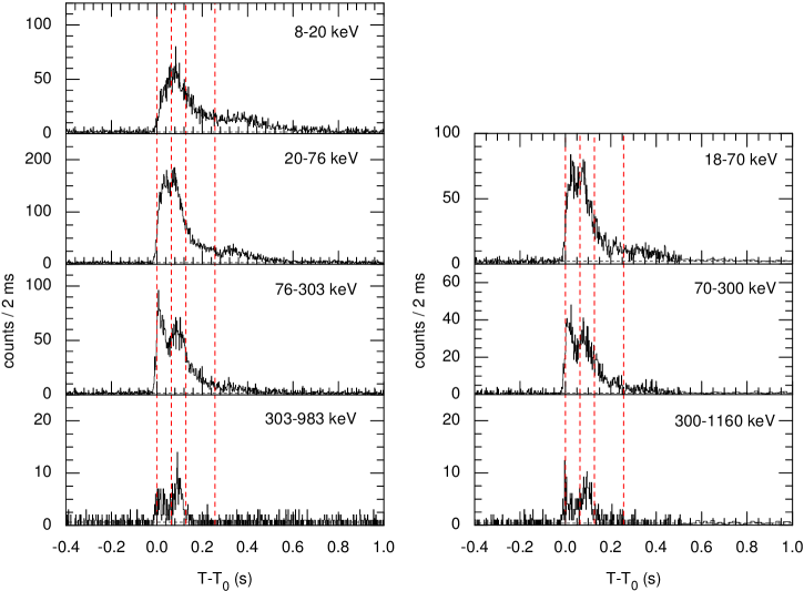
Figure 1.— GBM and Konus light curves of GRB $120323$A with 2 ms time resolution (left and right respectively) after accounting for light propagation between the two spacecrafts; Konus trigger time, T₀, is used as the time reference. Because of the 18 keV low energy threshold of Konus, no light curve is available for this instrument below this value. For clarity, we did not plotted the light curves beyond 1 MeV. Indeed, while GBM and Konus high energy thresholds are 40 MeV and 7 MeV, respectively, few data are available beyond 1 MeV for GRB $120323$A. The vertical dashed red lines mark the three time intervals used for the spectral analysis: sp1–4 (i.e., T₀ to T₀+0.256 s), sp1 (i.e., T₀ to T₀+0.064 s) and sp2 (i.e., T₀+0.064 s to T₀+0.128 s).

2. Observations

GRB $120323$A triggered GBM (Gruber & Connaughton, 2012) and Konus (Golenetskii et al., 2012a) on 2012 March 23 at 12:10:19.72 UT and 12:10:15.97 UT, respectively. This short and intense GRB has the highest peak flux among all short events observed with GBM thus far. While some emission can be observed up to several MeV with both GBM and Konus, this event is rather soft with the bulk of the emission below 100 keV. Despite an Autonomous Repointing Request (ARR) of the Fermi spacecraft triggered by the intensity of the event, the Fermi/Large Area Telescope (LAT) did not detect any significant emission even in the Low LAT Energy (LLE) data (20 to 100 MeV). Figure 1 shows the 2-ms time resolution light curves (LCs) of GRB $120323$A as observed with GBM (left) and with Konus (right) in energy bands ranging from 8 keV to 1 MeV. Due to the 18 keV energy threshold of Konus, the energy band 8-20 keV is missing for this instrument. The LCs of the two instruments are very similar above 20 keV exhibiting a sharp increase at the trigger time, two peaks with a separation of about 0.1s followed by a decaying tail with a small rebrightening from $\sim$0.30 to $\sim$0.40 s. The GBM LC below 20 keV exhibits one single peak with similar rising and decaying time up to 0.16 s followed by a decaying tail as observed in the other energy bands. The GBM and Konus T₉₀ durations in the 50-300 keV energy range (Kouveliotou et al., 1993) reported for this event were 0.448$\pm$0.090 s (Gruber & Connaughton, 2012) and $\sim$0.5 s (Golenetskii et al., 2012b), respectively.

The best location for this event was estimated with the Inter-Planetary Network (IPN) at RA=340.4^o, Dec=29.7^o, inside an irregular error box with a minimal and maximal dimension of 0.25^o and 0.75^o, respectively (Golenetskii et al., 2012a).

Table 1Spectral parameters and their 1–$\sigma$ confidence intervals resulting from CPL, Band, B+BB and C+BB fits to GRB $120323$A spectra in time intervals sp1–4, sp1 and sp2, using the GBM detectors n0, n1, n3, b0 and Konus data.

Model	Data Sets	Band or CPL			BB	EAC				pgstat/dof
	Parameters	Epeak	$\alpha$	$\beta$	kT	N0/B0	N1/B0	N3/B0	K/B0
sp1-4
CPL	GBM	196$\pm$14	-1.36$\pm$0.03	–	–	0.79$\pm$0.07	0.87$\pm$0.07	0.83$\pm$0.07	–	794/474
	GBM (20keV–7MeV)	231$\pm$23	-1.60$\pm$0.04	–	–	0.85$\pm$0.07	0.93$\pm$0.07	0.90$\pm$0.07	–	519/395
	Konus	316${}_{\mathrm{-40}}^{\mathrm{+55}}$	-1.51$\pm$0.07	–	–	–	–	–	–	49/43
	GBM+Konus	216$\pm$11	-1.40$\pm$0.03	–	–	0.79(fix)	0.87(fix)	0.83(fix)	0.72$\pm$0.03	883/522
Band	GBM	72$\pm$6	-0.66$\pm$0.09	-2.09$\pm$0.04	–	0.85$\pm$0.07	0.93$\pm$0.08	0.90$\pm$0.08	–	579/473
	GBM (20keV–7MeV)	108$\pm$13	-1.21$\pm$0.12	-2.20$\pm$0.09	–	0.79$\pm$0.08	0.86$\pm$0.08	0.83$\pm$0.08	–	484/394
	Konus	290${}_{\mathrm{-184}}^{\mathrm{+62}}$	-1.49${}_{\mathrm{-0.08}}^{\mathrm{+0.67}}$	-2.78${}_{\mathrm{-3.47}}^{\mathrm{+0.69}}$	–	–	–	–	–	46/42
	GBM+Konus	78$\pm$9	-0.75$\pm$0.05	-2.09$\pm$0.10	–	0.85(fix)	0.93(fix)	0.90(fix)	0.75$\pm$0.03	642/521
B+BB	GBM	326$\pm$36	-1.35$\pm$0.05	$<$-3.00	12.0$\pm$0.8	0.90$\pm$0.08	0.98$\pm$0.08	0.95$\pm$0.08	–	527/471
	GBM (20keV–7MeV)	325${}_{\mathrm{-37}}^{\mathrm{+48}}$	-1.49$\pm$0.08	$<$-3.00	13.2${}_{\mathrm{-1.2}}^{\mathrm{+1.7}}$	0.88$\pm$0.07	0.96$\pm$0.07	0.92$\pm$0.07	–	444/392
	Konus	386${}_{\mathrm{-76}}^{\mathrm{+102}}$	-1.46${}_{\mathrm{-0.12}}^{\mathrm{+0.15}}$	-2.99$\pm 0.52$	18.2${}_{\mathrm{-3.6}}^{\mathrm{+5.0}}$	–	–	–	–	31/40
	GBM+Konus	343$\pm$30	-1.37$\pm$0.05	$<$-3.91	12.4$\pm$0.8	0.90(fix)	0.98(fix)	0.95(fix)	0.79$\pm$0.03	577/519
C+BB	GBM	326$\pm$36	-1.34$\pm$0.05	–	12.0$\pm$0.8	0.90$\pm$0.08	0.98$\pm$0.08	0.95$\pm$0.08	–	527/472
	GBM (20keV-7MeV)	325${}_{\mathrm{-37}}^{\mathrm{+48}}$	-1.49$\pm$0.08	–	13.2${}_{\mathrm{-1.2}}^{\mathrm{+1.7}}$	0.88$\pm$0.07	0.96$\pm$0.07	0.92$\pm$0.07	–	444/393
	Konus	404${}_{\mathrm{-69}}^{\mathrm{+106}}$	-1.48${}_{\mathrm{-0.11}}^{\mathrm{+0.14}}$	–	18.5${}_{\mathrm{-3.6}}^{\mathrm{+5.0}}$	–	–	–	–	32/41
	GBM+Konus	346$\pm$30	-1.37$\pm$0.04	–	12.5$\pm$0.8	0.90(fix)	0.98(fix)	0.95(fix)	0.79$\pm$0.03	577/520
sp1
CPL	GBM	146$\pm 10$	-0.96$\pm$0.07	–	–	0.77$\pm$0.12	0.86$\pm$0.13	0.83$\pm$0.12	–	725/474
	Konus	249${}_{\mathrm{-38}}^{\mathrm{+58}}$	-1.44$\pm$0.13	–	–	–	–	–	–	44/26
	GBM+Konus	161$\pm$9	-1.06$\pm$0.05	–	–	0.77(fix)	0.86(fix)	0.83(fix)	0.73$\pm$0.04	821/505
Band	GBM	70$\pm$7	+0.07$\pm$0.06	-2.21$\pm$0.10	–	0.98$\pm$0.14	1.08$\pm$0.15	1.06$\pm$0.15	–	489/473
	Konus	70$\pm$10	+0.58$\pm$0.50	-2.11$\pm$0.12	–	–	–	–	–	15/25
	GBM+Konus	69$\pm$6	+0.08$\pm$0.17	-2.19$\pm$0.05	–	0.98(fix)	1.08(fix)	1.06(fix)	0.87$\pm$0.05	499/504
B+BB	GBM	366${}_{\mathrm{-58}}^{\mathrm{+82}}$	-1.18$\pm$0.10	$<$-3.00	15.3$\pm$1.0	1.08$\pm$0.12	1.20$\pm$0.14	1.17$\pm$0.14	–	489/471
	Konus	404${}_{\mathrm{-155}}^{\mathrm{+301}}$	-1.17$\pm 0.28$	-2.66$\pm$01.89	17.3${}_{\mathrm{-1.7}}^{\mathrm{+3.2}}$	–	–	–	–	15/23
	GBM+Konus	385${}_{\mathrm{-50}}^{\mathrm{+68}}$	-1.20$\pm$0.08	$<$-3.00	15.5$\pm$0.9	1.08(fix)	1.20(fix)	1.17(fix)	0.96$\pm$0.05	506/502
C+BB	GBM	366${}_{\mathrm{-58}}^{\mathrm{+83}}$	-1.18$\pm$0.10	–	15.3$\pm$1.0	1.08$\pm$0.14	1.19$\pm$0.15	1.17$\pm$0.15	–	489/472
	Konus	428${}_{\mathrm{-101}}^{\mathrm{+279}}$	-1.20${}_{\mathrm{-0.31}}^{\mathrm{+0.52}}$	–	17.4${}_{\mathrm{-2.2}}^{\mathrm{+3.1}}$	–	–	–	–	15/24
	GBM+Konus	385${}_{\mathrm{-50}}^{\mathrm{+68}}$	-1.21$\pm$0.09	–	15.5$\pm$0.9	1.08(fix)	1.19(fix)	1.17(fix)	0.96$\pm$0.05	506/503
sp2
CPL	GBM	314${}_{\mathrm{-39}}^{\mathrm{+52}}$	-1.50$\pm$0.04	–	–	0.77$\pm 0.08$	0.82$\pm 0.09$	0.80$\pm$0.09	–	678/474
	Konus	482${}_{\mathrm{-104}}^{\mathrm{+181}}$	-1.52$\pm$0.10	–	–	–	–	–	–	24/26
	GBM+Konus	345${}_{\mathrm{-33}}^{\mathrm{+41}}$	-1.52$\pm$0.03	–	–	0.77(fix)	0.82(fix)	0.80(fix)	0.62$\pm$0.04	710/505
Band	GBM (Option 1)	48$\pm$3	-0.14$\pm$0.30	-1.96$\pm$0.05	–	0.79$\pm$0.10	0.83$\pm$0.10	0.82$\pm$0.10	–	607/473
	” (Option 2)	314${}_{\mathrm{-39}}^{\mathrm{+52}}$	-1.50$\pm$0.03	$<$-6.92	–	0.77$\pm$0.08	0.82$\pm$0.09	0.80$\pm$0.09	–	678/473
	Konus	478${}_{\mathrm{-107}}^{\mathrm{+187}}$	-1.52$\pm$0.11	$<$-3.00	–	–	–	–	–	24/25
	GBM+Konus	48$\pm$3	-0.17$\pm$0.10	-1.93$\pm$0.20	–	0.79(fix)	0.83(fix)	0.82(fix)	0.61$\pm 0.04$	658/504
	”	345${}_{\mathrm{-33}}^{\mathrm{+41}}$	-1.52$\pm$0.03	$<$-3.00	–	0.77(fix)	0.82(fix)	0.80(fix)	0.62$\pm$0.04	709/504
B+BB	GBM	456${}_{\mathrm{-59}}^{\mathrm{+78}}$	-1.25$\pm$0.08	$<$-3.00	9.7$\pm$0.6	0.85$\pm$0.09	0.89$\pm$0.08	0.88$\pm$0.08	–	507/471
	Konus	482${}_{\mathrm{-60}}^{\mathrm{+72}}$	-1.28$\pm 0.10$	$<$-3.00	9.4${}_{\mathrm{-2.6}}^{\mathrm{+3.2}}$	–	–	–	–	21/23
	GBM+Konus	469${}_{\mathrm{-47}}^{\mathrm{+59}}$	-1.26$\pm$0.08	$<$-3.00	9.7$\pm$0.6	0.85(fix)	0.89(fix)	0.88(fix)	0.65$\pm$0.05	538/502
C+BB	GBM	456${}_{\mathrm{-59}}^{\mathrm{+78}}$	-1.25$\pm$0.08	–	9.7$\pm$0.6	0.85$\pm$0.09	0.89$\pm$0.08	0.88$\pm$0.08	–	507/472
	Konus	484${}_{\mathrm{-90}}^{\mathrm{+143}}$	-1.28${}_{\mathrm{-0.19}}^{\mathrm{+0.36}}$	–	9.4$\pm$2.0	–	–	–	–	21/24
	GBM+Konus	469${}_{\mathrm{-47}}^{\mathrm{+59}}$	-1.26$\pm$0.08	–	9.7$\pm$0.6	0.85(fix)	0.89(fix)	0.88(fix)	0.65$\pm$0.04	538/503

3. Data Analysis

For the analysis of GBM data, we use the same selection criteria (i.e., data file type, detectors and energy selection) as described in Section 3 of Guiriec et al. (2013) as well as the same response files generated using the IPN location and the same background estimate. Konus data are extracted from detector S2 in two overlapping energy ranges covering from 20 keV to 16 MeV: 20 keV–1.6 MeV (i.e., high-gain PHA1) and 450 keV–16 MeV (i.e., low-gain PHA2). We exclude PHA1 data beyond 450 keV from the analysis to avoid duplication in the PHA1-PHA2 joint spectral fit process. No statistically significant emission is detected in Konus spectral channels beyond 7 MeV, which justifies the 7 MeV high energy cut used later on in this article.

The background of PHA1 and PHA2 data for GRB $120323$A is modeled as a constant using the total counts accumulated from T₀+25 s to T₀+254 s. Located at L1 Lagrange point, Konus data are not affected by the same intense flux of charged particles captured in Earth’s magnetic field that strongly affect the GBM background (low Earth orbit). The Konus background is, therefore, usually more stable. However, the very short duration of GRB $120323$A strongly reduces possible systematic effects in the background estimate used for the analysis of GBM data.

The full energy resolution of the Konus data is only available with a 64 ms time resolution. Therefore, this time resolution is the most constraining factor when defining time intervals for the joint GBM and Konus time resolved spectral analysis. We extracted GBM spectral data in the same four time intervals as those imposed by the Konus time resolution in taking into account the light propagation time between the Fermi and Wind spacecrafts. We performed a time-integrated spectral analysis of GRB $120323$A over these four time intervals of Konus (later sp1–4) and a time resolved spectral analysis of the first two: 0–64 ms (later sp1) corresponding mostly to the first peak of the LC observed above 20 keV, and 64–128 ms (later sp2) corresponding mostly to the second peak (see Figure 1). The last two intervals correspond to the decay phase of the burst; we did not perform spectral analysis in each of them individually because their signal is weak. The vertical dashed red lines on Figure 1 indicate the three time intervals used in this analysis: sp1–4, sp1 and sp2.

We fitted the C_nTh1+C_Th model (Guiriec et al., 2011, 2013, 2015a, 2015b, 2016a, 2016b)—where C_nTh1 is a non-thermal component that we approximate with a Band function or a power law with an exponential cutoff (CPL), and C_Th is a thermal-like component that we approximate with $\emptyset$ or a black body (BB)—to the data in each time interval using either Konus and GBM data separately or together in a joint fit. In this analysis we only consider the best models reported in Guiriec et al. (2013) to compare Konus results to GBM ones. To perform the spectral analysis, we used the software package XSpec and the best fit parameters as well as their corresponding uncertainties were estimated by minimizing PGSTAT (i.e., Poisson-Gaussian Statistic). This statistic is particularly interesting when fitting data in different statistical count regimes. The energy channels are grouped in order to have at least 1 count per energy bin as recommended for optimal usage of PGSTAT; the energy bins in the Konus data have typically more than 20 counts per bin.

While the two data sets of Konus are calibrated prior to the spectral analysis, no specific calibration is performed between the NaI and BGO detectors of GBM. Therefore, when fitting GBM data alone, we apply an effective area correction (EAC) factor between each NaI detector and BGO 0 (BGO 0 being the reference). This gives three additional free parameters to the fit of GBM data alone. When fitting simultaneously GBM and Konus data (later GBM+Konus), the EAC factors between BGO and NaI detectors are fixed to the values obtained from the best fit to the GBM data alone using the respective model. Therefore, GBM detectors are considered as a single instrument such as Konus. An EAC factor is then applied in between BGO 0 and Konus data to measure possible discrepancies in the flux estimates between the two instruments.

The analysis results are reported in Table 1, Figure 2 and Figures A1 to A3.

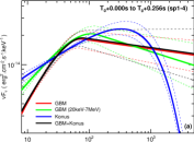
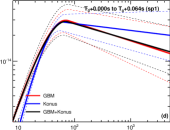
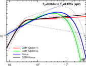
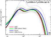
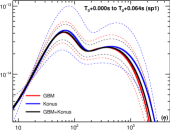
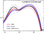
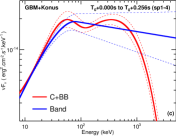
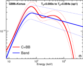
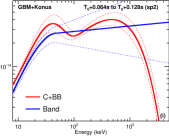
Figure 2.— Band function (top line panels) and C+BB models (middle line panels) resulting from the fit of GBM, Konus and GBM+Konus data in time intervals sp1–4, sp1 and sp2 (left to right column, respectively). The solid lines correspond to the function resulting from the best fit parameters while the dashed lines correspond to the 1–$\sigma$ confidence region for the fit. The panels in the bottom line correspond to the Band functions overplotted with the C+BB models obtained when fitting jointly GBM and Konus data. The spectral shape resulting from the fit of the Konus data only are renormalized using the EAC correction factor estimated when fitting jointly GBM+Konus data with the same function and in the same time interval (see Table 1).

4. Results

4.1. Time-Integrated Spectral Analysis

The Band function (Band et al., 1993) fits to the GBM and Konus data separately in time interval sp1–4 result in two dramatically different spectral shapes (see red and blue lines in Figure 2a, and Table 1). While the E_peak value measured by GBM is very low for such a bright and short GRB ($\sim$80 keV), the Konus measurement is quite typical ($\sim$300 keV). Also, the value of the spectral index $\alpha$ of the Band function estimated with Konus data ($\alpha$$\sim$$-$1.50) is significantly lower than the one measured with GBM data ($\alpha$$\sim$$-$0.66).

We investigated the possible impact of the difference in the energy ranges covered by the two instruments to explain the observed discrepancies. To do so, we fitted the GBM data over the same energy range as Konus (i.e., from 20 keV to 7 MeV). In reducing the GBM energy range we obtain a higher value for E_peak compared to the fit to GBM data over the whole energy range of the instrument, as well as lower values for $\alpha$ and $\beta$ (see green line in Figure 2a and Table 1). This fit result is intermediate between the fit of GBM data over its full energy range and the fit of Konus data. This is an indication that the extended energy range covered by GBM can strongly impact the fit results, and it may explain, at least in part, the discrepancies observed between the two instruments. We note that the high-energy power law of the Band function systematically overshoots the BGO data at the highest energies showing that the Band function alone is unable to adequately capture the spectral shape of the GBM data over its whole energy range (see Figure A1).

When fitting GBM and Konus data simultaneously, the resulting Band function is similar to the one obtained when fitting GBM data alone (see black line in Figure 2a); this is because GRB $120323$A is much more intense in GBM than in Konus. While EAC factors of only a few percent are required between NaI and BGO detectors when fitting a Band function to the GBM data alone, 20 to 30% correction is necessary to align the GBM and Konus fluxes (see Table 1).

Conversely to the results reported for the Band only fits, the C_nTh1+C_Th fits (with C_nTh1 being either Band or CPL, and C_Th being BB) to the GBM and Konus data alone or together lead to consistent spectral shapes (see Table 1 and Figure 2b).

In the C_nTh1+C_Th model, the shape of C_nTh1 is similar to the one obtained when fitting Band alone to the Konus data, and the shape of C_Th mimics the Band function fit to the GBM (or GBM+Konus) data with E_peak matching with the BB spectrum peak energy (see Figure 2c). We can also note that no correction is necessary between NaI and BGO data when fitting C_nTh1+C_Th to the GBM data, and the correction between GBM and Konus is reduced by a few percent.

Moreover, the spectral shapes obtained with Band+BB and CPL+BB are identical (the parameter values and the fit statistics), so henceforth we will only consider CPL+BB when comparing models since it has one degree of freedom (later dof) less. The improvements in the PGSTAT values (later $\Delta$PGSTAT) between C_nTh1+C_Th and Band fits are 52, 14 and 65 units for one additional dof. for GBM, Konus and GBM+Konus data, respectively. In the three cases, this is a statistically significant improvement making C_nTh1+C_Th the best model with the lower number of free parameters.

4.2. Time-Resolved Spectral Analysis

We performed a similar analysis as the one presented in Section 4.1 for the time intervals sp1 and sp2. The data, the residuals of the fits and the fit results are presented in Table 1, Figure 2 and Figures A2 and A3 for sp1 and sp2, respectively.

The fits to Band functions alone to the GBM, Konus and GBM+Konus data in sp1 are globally consistent (see Figure 2d and Table 1). The three fits are characterized by low E_peak values around 70 keV and positive values for $\alpha$. In addition, the value of $\alpha$ is significantly higher for Konus data than for GBM. Such high values of $\alpha$ point toward a thermal origin of the emission process. This is in good agreement with the results reported in Guiriec et al. (2013).

The parameter values of C_nTh1 in C_nTh1+C_Th are totally incompatible with those obtained when fitting Band alone to the data (see Figure 2f and Table 1). Whatever data set is used—GBM, Konus or GBM+Konus—the values of E${}_{\mathrm{peak}}^{nTh1}$ are much higher than the values of E${}_{\mathrm{peak}}^{Band}$, and the values of $\alpha_{nTh1}$ ($\alpha_{nTh1}$$\sim$$-$1.2) are much lower than the values of $\alpha_{Band}$ ($>$0).

Similarly, the high-energy spectral slope of C_nTh1 is much steeper than the one resulting from the Band only fit (i.e., $\beta$) and cannot be differentiated from an exponential cutoff based on our data sets. Therefore, CPL+BB is equivalent to Band+BB (for both the parameters of the components and the statistical results), and since CPL+BB has one free parameter less than Band+BB, we will consider this model for statistical comparison.

Figure 2e shows the very good consistency of the C_nTh1+C_Th fits for the three data sets with the confidence region progressively decreasing from the Konus fit alone to the GBM fit alone to the GBM+Konus fit. A C_Th temperature of $\sim$16 keV is obtained with the three data sets. Once more, these results are consistent with the analysis presented in Guiriec et al. (2013).

For the three data sets (i.e., GBM, Konus and GBM+Konus), the Band and C_nTh1+C_Th (i.e., Band+BB or CPL+BB) fits result in similar PGSTAT values. If the parameters of the Band function in the Band-only fits and of C_nTh1 in C_nTh1+C_Th were identical, it would indicate that the additional parameters introduced with C_Th are not required to improve the fits, and the intensity of this component should then be compatible with zero. Here, the shape of the Band functions and of C_nTh1 resulting from the Band-only and C_nTh1+C_Th fits, respectively, are dramatically different, and in the C_nTh1+C_Th scenario, C_Th is an intense component which overpowers C_nTh1 between 20 and 150 keV. From this result, we conclude that given the quality of our data sets, a spectral shape with two humps (i.e., C_nTh1+C_Th) describes the data in sp1 as well as a spectral shape with a single hump (i.e., Band). However, the positive values of the low energy spectral indices in both scenarios require a thermal emission process. This is again in good agreement with the results reported in Guiriec et al. (2013). Indeed, the authors reported no statistically significant improvement of C_nTh1+C_Th over Band in the first peak of the LC, but strong changes in the parameters of the Band function pointing to a thermal emission origin for the two scenarios.

When Band or C_nTh1+C_Th are fitted to the GBM data of sp1, no EAC is required between NaI and BGO detectors within the 1–$\sigma$ uncertainties. Similarly, the C_nTh1+C_Th fits to the GBM+Konus data do not require any correction between GBM and Konus. However, a flux correction $>$12% is required in the case of the Band-only fit. This shows once more that GBM and Konus data are fully consistent only when using C_nTh1+C_Th.

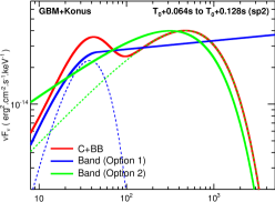
Figure 3.— Best C+BB fit (red line) and the two options for the Band function fits (solid blue and green lines for options 1 and 2, respectively) to GBM+Konus data in the time interval sp2. The dashed blue and green lines correspond to the BB and CPL components of the C+BB model, respectively.

In time interval sp2, the C_nTh1+C_Th fits to GBM, Konus and GBM+Konus data give consistent results with a temperature of $\sim$10 keV for the BB, E_peak around 400–500 keV, $\alpha$ around -1.2 and a very steep slope for the high energy PL making Band+BB similar to CPL+BB (see Table 1 and Figure 2h); this is good agreement with the results reported in Guiriec et al. (2013). The spectral parameters obtained when fitting C_nTh1+C_Th to the data in sp1 and sp2 are very similar. This is not the case when considering the Band-only fits for which the parameters are dramatically different between sp1 and sp2.

Interestingly, the minimization of a Band function alone to either GBM or GBM+Konus data converges towards two possible minima corresponding to dramatically different spectral parameters (see Table 1 and Figures 2g and 3): the solution called Option 1 has a lower PGSTAT value than the solution called Option 2. In Figure 3, we overplot in solid lines the C_nTh1+C_Th best fit (red) to GBM+Konus data as well as the two options for the Band function (blue and green for options 1 and 2, respectively). The dashed blue and green lines correspond to the C_Th and C_nTh1 components of the C_nTh1+C_Th model, respectively. We note the strong similarities of the solid and dashed blue lines up to $\sim$35 keV as well as the similarities of the solid and dashed green lines especially above $\sim$300 keV. Therefore, Option 1 mimics clearly the low-energy hump of the C_nTh1+C_Th model (i.e., C_Th) while Option 2 mimics the high-energy hump of C_nTh1+C_Th (i.e., C_nTh1).

A $\Delta$PGSTAT of 100, 3 and 120 is obtained between Band and C_nTh1+C_Th with GBM, Konus and GBM+Konus data, respectively, showing that C_nTh1+C_Th is statistically significantly better than Band in the time interval sp2 only with GBM data. The limited improvement obtained with Konus can be explained by a weaker signal detected with Konus as well as with the Konus energy band pass starting at 20 keV while the peak energy of the BB is at $\sim$30 keV (see Figure 3). Once more, the results obtained in sp2 using GBM, Konus and GBM+Konus data globally support those reported in Guiriec et al. (2013).

While a limited correction of order of a few percent may be needed to reconcile NaI and BGO detector fluxes in sp2, a $\sim$30% correction is needed in between GBM and Konus. In sp2, fluxes obtained with BGO seem to be systematically higher than those obtained with NaI detectors and Konus. As in sp1, this correction factor required to re-normalize the fluxes for the joint analysis in sp2 does not impact the very good consistency of the parameters resulting from the C_nTh1+C_Th fits when analyzing GBM and Konus data either separately or jointly.

5. Conclusion

Through the time-integrated and the coarse time-resolved spectral analysis of GRB $120323$A using GBM and Konus data fitted either jointly or separately, we found consistency of the data sets from these two different instruments. However, although the spectral parameters are similar when fitting the data from one instrument or the other, a normalization correction factor which can reach up to 30% must be applied to calibrate the fluxes, Konus flux estimation being lower than GBM one. A few % correction may also be applied in some cases to renormalize fluxes between NaI and BGO detectors. BGO 0 seems to systematically predict higher fluxes than the selected sample of NaI detectors and Konus. While the Band function fit to the data of GBM and Konus separately can lead to strong discrepancies in the resulting spectral parameters, C_nTh1+C_Th results in fits that are perfectly compatible for the two instruments.

Overall, the fits obtained in this analysis are very similar to those presented in Guiriec et al. (2013) who fitted coarse time intervals. Unfortunately, it is not possible to perform time resolved spectral analysis of Konus data using as fine time intervals as in Guiriec et al. (2013) due to the limited time resolution of Konus compared to GBM. Such fine time-resolved spectroscopy was crucial to track the evolution of the components with time, which is an important argument supporting the existence of these two components. Discontinuities were indeed found in the temporal evolution of the parameters of the Band function when Band-alone was fitted to high time resolution data. Such discontinuities are difficult to interpret on physical ground. On another hand, spectral fits using two humps (i.e., C_nTh1+C_Th) did not show any discontinuities and the values of the parameters of C_nTh1 were very much compatible with synchrotron emission from electrons in fast-cooling regime. We observed similar results when comparing time interval sp1 and sp2 in Section 4.2. However, with only two time intervals, this result does not appear as clear as in Guiriec et al. (2013).

In addition, fine time-resolved spectral analysis also revealed a relation between the instantaneous luminosity of C_nTh1, L${}_{i}^{nTh1}$, and the corresponding instantaneous $\nu$F_ν peak energy, E${}_{\mathrm{peak,i}}^{nTh1}$ (i.e., L${}_{i}^{nTh1}$–E${}_{\mathrm{peak,i}}^{nTh1}$ relation) only when fitting C_nTh1+C_Th to the data, these two quantities being uncorrelated when fitting Band alone. Even with the coarse resolution of the Konus data our results confirm the analysis performed in Guiriec et al. (2013), establishing two humps in the prompt emission spectra of GRB $120323$A . We interpret this double hump structure as resulting from two separate components (i.e., C_nTh1+C_Th), one with a thermal-like shape, C_Th (most-likely of photospheric origin) and the other one with a non-thermal shape, C_nTh1 (possibly of synchrotron origin from electrons beyond the photosphere).

Our results show the importance of using the correct spectral model to intercalibrate data sets from different instruments. Despite the very good consistency of the spectral shapes resulting from the C_nTh1+C_Th fits to the GBM and Konus data, our results reveal flux normalization discrepancies between the two instruments. To efficiently intercalibrate Konus and GBM, we would need to analyze a larger data set of common events.

6. Acknowledgments

To Neil Gehrels; you are an exceptional scientist, mentor, leader, friend and human being. Your support has always been instrumental to the success of this project. You are loved and missed.

We thank the Konus team and in particular D. Frederiks, V. Pal’shin and D. Svinkin for extracting the Konus data used in this study, for providing the time correction corresponding to the light propagation between Fermi and Wind, and for their useful comments and suggestions that significantly improved the quality of the article. To complete this work, SG was supported by the NASA Postdoctoral Program (NPP) at the NASA/Goddard Space Flight Center, administered by Oak Ridge Associated Universities through a contract with NASA. SG acknowledges financial support through the Cycles-5,7 and 9 NASA Fermi Guest Investigator program (NNH11ZDA001N #51279, #71377 and #91264) to complete this work as part of a larger project.

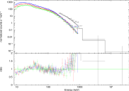
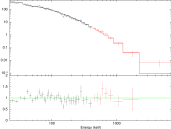
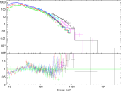
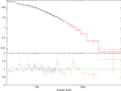
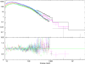
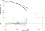
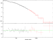
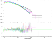
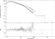
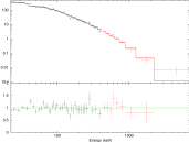
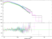
Figure A1.— GBM, Konus and GBM+Konus count-rate spectra (left, center and right columns, respectively) in time interval sp1–4 (T₀ to T₀+0.256 s) with the residuals resulting from the CPL, Band, B+BB and C+BB fits (lines 1 to 4 from top to bottom, respectively). GBM energy channels have been grouped in larger energy bins for display purpose only; this grouping does not affect the fitting process that uses the best energy resolution of the instrument.

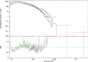
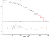
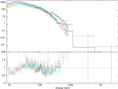
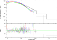
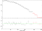
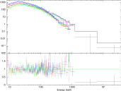
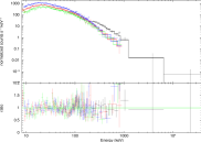
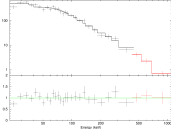
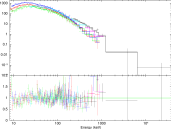
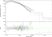
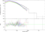
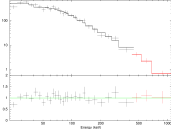
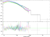
Figure A2.— GBM, Konus and GBM+Konus count data (left, center and right columns, respectively) in time interval sp1 (T₀ to T₀+0.064 s) with the residuals resulting from the CPL, Band, B+BB and C+BB fits (lines 1, 2, 3-4 and 5 from top to bottom, respectively). GBM energy channels have been grouped in larger energy bins for display purpose only; this grouping does not affect the fitting process that uses the best energy resolution of the instrument.

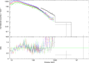
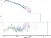
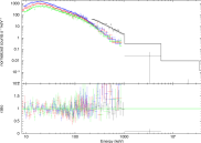
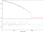
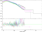
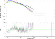
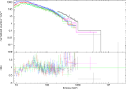
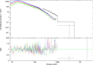
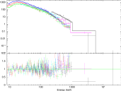
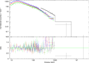
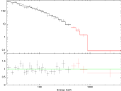
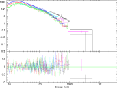
Figure A3.— GBM, Konus and GBM+Konus count data (left, center and right columns, respectively) in time interval sp2 (T₀+0.064 s to T₀+0.128 s) with the residuals resulting from the CPL, Band, B+BB and C+BB fits (lines 1, 2-3, 4 and 5 from top to bottom, respectively). GBM energy channels have been grouped in larger energy bins for display purpose only; this grouping does not affect the fitting process that uses the best energy resolution of the instrument.

References

- Band et al. (1993) Band, D., Matteson, J., Ford, L., et al.: 1993, ApJ, 413, 281
- Golenetskii et al. (2012a) Golenetskii, S., et al.: 2012a, GCN, 13102, 1
- Golenetskii et al. (2012b) Golenetskii, S., et al.: 2012b, GCN, 13103, 1
- Gruber & Connaughton (2012) Gruber, D., & Connaughton, V.: 2012, GCN, 13099, 1
- Guiriec et al. (2010) Guiriec, S., Briggs, M. S., Connaugthon, V., et al. 2010, ApJ, 725, 225
- Guiriec et al. (2011) Guiriec, S., Connaughton, V., Briggs, M. S., et al. 2011, ApJ, 727, L33
- Guiriec et al. (2013) Guiriec, S., Daigne, F., Hascoët, R., et al. 2013, ApJ, 770, 32
- Guiriec et al. (2015a) Guiriec, S., Kouveliotou, C., Daigne, F., et al. 2015a, ApJ, 807, 148
- Guiriec et al. (2015b) Guiriec, S., Mochkovitch, R., Piran, T., et al. 2015b, ApJ, 814, 10
- Guiriec et al. (2016a) Guiriec, S., Gonzalez, M. M., Sacahui, J. R., et al. 2016a, ApJ, 819, 79
- Guiriec et al. (2016b) Guiriec, S., Kouveliotou, C., Hartmann, D. H., et al. 2016b, ApJ, 831, L8
- Kouveliotou et al. (1993) Kouveliotou, C., et al.: 1993, ApJ, 413, L101
- Svinkin et al. (2016) Svinkin, D. S., Frederiks, D. D., Aptekar, R. L., et al. 2016, ApJS, 224, 10