h KA-TP-10-2017
h DESY 17-046
Phenomenological Comparison of Models with Extended Higgs Sectors

Abstract

Beyond the Standard Model (SM) extensions usually include extended Higgs sectors. Models with singlet or doublet fields are the simplest ones that are compatible with the $\rho$ parameter constraint. The discovery of new non-SM Higgs bosons and the identification of the underlying model requires dedicated Higgs properties analyses. In this paper, we compare several Higgs sectors featuring 3 CP-even neutral Higgs bosons that are also motivated by their simplicity and their capability to solve some of the flaws of the SM. They are: the SM extended by a complex singlet field (CxSM), the singlet extension of the 2-Higgs-Doublet Model (N2HDM), and the Next-to-Minimal Supersymmetric SM extension (NMSSM). In addition, we analyse the CP-violating 2-Higgs-Doublet Model (C2HDM), which provides 3 neutral Higgs bosons with a pseudoscalar admixture. This allows us to compare the effects of singlet and pseudoscalar admixtures. Through dedicated scans of the allowed parameter space of the models, we analyse the phenomenologically viable scenarios from the view point of the SM-like Higgs boson and of the signal rates of the non-SM-like Higgs bosons to be found. In particular, we analyse the effect of singlet/pseudoscalar admixture, and the potential to differentiate these models in the near future. This is supported by a study of couplings sums of the Higgs bosons to massive gauge bosons and to fermions, where we identify features that allow us to distinguish the models, in particular when only part of the Higgs spectrum is discovered. Our results can be taken as guidelines for future LHC data analyses, by the ATLAS and CMS experiments, to identify specific benchmark points aimed at revealing the underlying model.

1 Introduction

While the discovery of the Higgs boson by the LHC experiments ATLAS [1] and CMS [2] has been a great success for particle physics and the Standard Model (SM) in particular, the unsolved puzzles of the SM call for New Physics (NP) extensions beyond the SM (BSM). Since we are still lacking any direct discovery of BSM physics, the Higgs sector itself has become a tool in the search for NP. The latter can manifest itself in various ways [3]. The discovery of additional Higgs bosons or the measurement of new sources of CP violation in the Higgs sector would be a direct observation of BSM physics. Indirect hints would be given by deviations of the Higgs couplings from the SM expectations. As the discovered Higgs boson behaves very SM-like [4, 5, 6, 7] the revelation of such deviations requires, on the one hand, very precise measurements from the experiments and, on the other hand, very precise predictions from the theory side. In parallel to the increase in precision, observables have to be identified that allow for the identification of NP, in particular the nature of the underlying model. Thus, the pattern of the coupling deviations gives information on the specific model that may be responsible. Production rates may be exploited to exclude some of the models or to single out the model realized in nature. In the ideal case smoking gun signatures are identified that unmask the model behind NP.

The immense amount of possible BSM Higgs sectors calls for a strategy on the choice of the models to be investigated. Any NP model has to provide a Higgs boson with a mass of 125.09 GeV [8] that behaves SM-like. The model has to fulfil the exclusion bounds from Higgs and NP searches, the $B$-physics and various low-energy constraints and to be compatible with the electroweak precision data. Furthermore, the theoretical constraints on the Higgs potential, i.e. that it is bounded from below, that the chosen vacuum is the global minimum at tree level and that perturbative unitarity holds, have to be fulfilled. Among the weakly coupled models those with singlet or doublet extended Higgs sectors belong to the simplest extensions that comply with the $\rho$ parameter constraint. For this class of models we have analysed, in previous works, their distinction based on collider phenomenology. In [3] we studied the implications of precision measurements of the Higgs couplings for NP scales and showed how coupling sum rules can be used to tell the Next-to-Minimal Supersymmetric extension (NMSSM) from the Minimal Supersymmetric extension (MSSM). We reassessed this question in [9] in the framework of specific NMSSM benchmarks. In [10], for the 2-Higgs-Doublet Model (2HDM), and in [11], for the NMSSM, we demonstrated how the simultaneous measurements of Higgs decays involving the 125 GeV Higgs boson, the $Z$ boson and one additional Higgs boson undoubtedly distinguish a CP-violating from a CP-conserving Higgs sector. In [12] we found that the distinction of the complex-singlet extended SM (CxSM) from the NMSSM based on Higgs-to-Higgs decays is only possible through final states with two different scalars. The authors of [13, 14] attacked the task of differentiating NP at the LHC from a different perspective by asking how well the Higgs mass and couplings need to be measured to see deviations from the SM. In a similar spirit we investigated in [15] if NP could first be seen in Higgs pair production taking into account Higgs coupling constraints.

In this work we elaborate further on the distinction of NP models based on LHC collider phenomenology. We go beyond our previous works by comparing a larger class of models that are, to some extent, similar in their Higgs sector but involve different symmetries. We explore how this manifests in the Higgs phenomenology and how it can be exploited to differentiate the models. With the guiding principle that the models are able to solve some of the questions of the SM while remaining compatible with the given constraints, we investigate in this work the simplest extensions featuring 3 neutral CP-even Higgs bosons. This particular scenario is phenomenologically interesting because it allows for Higgs-to-Higgs decays into final states with two different Higgs bosons that lead to rather high rates, see e.g. [12]. At the same time we go beyond the largely studied minimal versions with 2 neutral CP-even Higgs bosons, the 2HDM and the MSSM. We will investigate the CxSM (the SM extended by a complex singlet field) in its broken phase, [16, 12], the Next-to-Minimal 2HDM (N2HDM, the 2HDM [17, 18, 19] extended by a singlet field) [20, 21, 22, 23, 24, 25, 26, 27, 28, 29, 30, 31, 32, 33], and, as representative for a supersymmetric (SUSY) model, the NMSSM [34, 35, 36, 37, 38, 39, 40, 41, 42, 43, 44, 45, 46, 47, 48, 49]. While in all three models the singlet admixture to the Higgs mass eigenstates decreases their couplings to the SM particles, they are considerably different: The NMSSM is subject to SUSY relations to be fulfilled while the CxSM is much simpler than the N2HDM and NMSSM, which contain a charged Higgs boson and, additionally, one and two CP-odd Higgs bosons, respectively. We will also compare the phenomenological effects of coupling modifications through singlet admixture with the corresponding effects caused by CP violation. For this purpose we include the complex 2HDM (C2HDM) [50, 51, 52, 53, 54, 55, 21, 56, 57, 58] in our study. In this model all 3 neutral Higgs bosons mix to form CP-violating mass eigenstates, in contrast to the real 2HDM which features 2 CP-even and 1 CP-odd Higgs boson. The measurement of CP violation is experimentally very challenging and, at a first stage, in the discovery of the neutral Higgs bosons of the C2HDM they can be misidentified as CP-even or CP-odd Higgs bosons. In such an experimental scenario we have a clear connection to our other CP-conserving models that also contain three neutral Higgs bosons mixing. This allows us to compare the effect of the singlet admixtures with the effect of CP violation on the Higgs couplings and associated physical processes. These two different ways of achieving coupling modifications may induce a considerably different Higgs phenomenology that might then be revealed by the appropriate observables. Finally, all these models may solve problems of the SM. Depending on the model and (possibly) on its spontaneous symmetry breaking phase it may e.g. provide a Dark Matter (DM) candidate, lead to successful baryogenesis, weaken the hierarchy problem or solve the $\mu$ problem of the MSSM [17, 59, 60, 61].

For all investigated models we will perform parameter scans by taking into account the experimental and theoretical constraints. We will investigate the mass distributions and the properties of the 125 GeV Higgs boson as a function of the singlet admixture and of the pseudoscalar admixture, respectively. We will study the production rates of the non-SM Higgs bosons and investigate Higgs coupling sums. We aim to answer the following questions: To which extent can LHC Higgs phenomenology, in particular signal rates and coupling measurements, be exploited to distinguish between these models with extended Higgs sectors? Are we able to disentangle the models based on Higgs rate measurements? Can the pattern of the couplings of the discovered Higgs bosons point towards possibly missing Higgs bosons in case not all of them have been discovered? Is it even possible to use coupling sums to reveal the underlying model? Can the investigation of the couplings give hints on the underlying NP scale? With our findings we hope to encourage the experiments to conduct specific phenomenological analyses and investigate the relevant observables. We aim to contribute to the endeavour of revealing the underlying NP model (if realized in nature) by using all the available data from the LHC experiments.

The outline of the paper is as follows. In section 2 we will present our models and introduce our notation. Section 3 describes the scans with the applied constraints. With section 4 we start our phenomenological analysis. After presenting the mass distribution of the Higgs spectra of our models, the phenomenology of the SM-like Higgs boson will be described. In Sect. 5 the signal rates of the non-SM-like Higgs bosons will be presented and discussed. Section 6 is dedicated to the investigation of the couplings sums. Our conclusions are given in Sect. 7.

2 Description of the Models

In this section we describe the models that we investigate. We start with the simplest one, the SM extended by a complex singlet field, the CxSM. We then move on in complexity with the (C)2HDM, the N2HDM and the NMSSM. We use this description also to set our notation.

2.1 The Complex Singlet Extension of the SM

In the CxSM a complex singlet field

$$\mathbb{S}=S+iA$$ (2.1)

with hypercharge zero is added to the SM Lagrangian. We study the CxSM since the simpler extension by a real singlet field, the RxSM, features only two Higgs bosons. The scalar potential with a softly broken global $U(1)$ symmetry is given by

$$V=\frac{m^{2}}{2}H^{\dagger}H+\frac{\lambda}{4}(H^{\dagger}H)^{2}+\frac{\delta_{2}}{2}H^{\dagger}H|\mathbb{S}|^{2}+\frac{b_{2}}{2}|\mathbb{S}|^{2}+\frac{d_{2}}{4}|\mathbb{S}|^{4}+\left(\frac{b_{1}}{4}\mathbb{S}^{2}+a_{1}\mathbb{S}+c.c.\right)\,,$$ (2.2)

with the soft-breaking terms in parenthesis. The doublet and complex singlet fields can be written as

$$H=\dfrac{1}{\sqrt{2}}\left(\begin{array}[]{c}G^{+}\\ v+h+iG^{0}\end{array}\right)\quad\mbox{and}\quad\mathbb{S}=\dfrac{1}{\sqrt{2}}\left[v_{S}+s+i(v_{A}+a)\right]\;,$$ (2.3)

where $v\approx 246$ GeV denotes the vacuum expectation value (VEV) of the SM Higgs boson $h$ and $v_{S}$ and $v_{A}$ are the real and imaginary parts of the complex singlet field VEV, respectively. We impose a $\mathbb{Z}_{2}$ symmetry on $A$, which is equivalent to a symmetry under $\mathbb{S}\to\mathbb{S}^{*}$. This forces $a_{1}$ and $b_{1}$ to be real. The remaining parameters $m,\lambda,\delta_{2},b_{2}$ and $d_{2}$ are required to be real by hermiticity of the potential. There are two possible phases consistent with electroweak symmetry breaking (EWSB) [16]. The symmetric (or DM) phase, with $v_{A}=0$ and $v_{S}\neq 0$, features only two mixed states plus one DM candidate, so we focus instead on the broken phase. In the latter all VEVs are non-vanishing and all three scalars mix with each other. Introducing the notation $\rho_{1}\equiv h$, $\rho_{2}\equiv s$ and $\rho_{3}\equiv a$, their mass matrix is obtained from the potential in the physical minimum through ($i,j=1,2,3$)

$$({\cal M}^{2})_{ij}=\left\langle\frac{\partial^{2}V}{\partial\rho_{i}\partial\rho_{j}}\right\rangle\;,$$ (2.4)

where the brackets denote the vacuum. The three mass eigenstates $H_{i}$ are obtained from the gauge eigenstates $\rho_{i}$ by means of the rotation matrix $R$ as

$$\left(\begin{array}[]{c}H_{1}\\ H_{2}\\ H_{3}\end{array}\right)=R\left(\begin{array}[]{c}\rho_{1}\\ \rho_{2}\\ \rho_{3}\end{array}\right)\,,$$ (2.11)

with

$$R\,{\cal M}^{2}\,R^{T}=\textrm{diag}\left(m_{H_{1}}^{2},m_{H_{2}}^{2},m_{H_{3}}^{2}\right),$$ (2.12)

and $m_{H_{1}}\leq m_{H_{2}}\leq m_{H_{3}}$ denoting the masses of the neutral Higgs bosons. Introducing the abbreviations $s_{i}\equiv\sin\alpha_{i}$ and $c_{i}\equiv\cos\alpha_{i}$ with

$$-\frac{\pi}{2}\leq\alpha_{i}<\frac{\pi}{2}\,,$$ (2.13)

the mixing matrix $R$ can be parametrized as

$$R=\left(\begin{array}[]{ccc}c_{1}c_{2}&s_{1}c_{2}&s_{2}\\ -(c_{1}s_{2}s_{3}+s_{1}c_{3})&c_{1}c_{3}-s_{1}s_{2}s_{3}&c_{2}s_{3}\\ -c_{1}s_{2}c_{3}+s_{1}s_{3}&-(c_{1}s_{3}+s_{1}s_{2}c_{3})&c_{2}c_{3}\end{array}\right)\;.$$ (2.17)

The model has seven independent parameters, and we choose as input parameters the set

$$\alpha_{1}\;,\quad\alpha_{2}\;,\quad\alpha_{3}\;,\quad v\;,\quad v_{S}\;,\quad m_{H_{1}}\quad\mbox{and}\quad m_{H_{3}}\;.$$ (2.18)

The VEV $v_{A}$ and the mass $m_{H_{2}}$ are dependent parameters. In the scans that we will perform they are determined internally by the program ScannerS [16, 62] in accordance with the minimum conditions of the vacuum.

The couplings $\lambda_{i}^{(p)}$ of the Higgs mass eigenstates $H_{i}$ to the SM particles, denoted by $p$, are all modified by the same factor. In terms of the couplings $\lambda_{h_{\text{SM}}}^{(p)}$ of the SM Higgs boson $h_{\text{SM}}$ they read

$$\lambda_{i}^{(p)}=R_{i1}\lambda_{h_{\text{SM}}}^{(p)}\;.$$ (2.19)

The trilinear Higgs self-couplings are obtained from the terms cubic in the fields in the potential $V$ of Eq. (2.2) after expanding the doublet and singlet fields about their VEVs and rotating to the mass eigenstates. Their explicit expressions together with the quartic couplings can be found in appendix B.1 of [12]. If kinematically allowed, the trilinear Higgs couplings induce Higgs-to-Higgs decays that change the total widths of the $H_{i}$ and hence their branching ratios to the SM particles. The branching ratios including the state-of-the art higher order QCD corrections and possible off-shell decays can be obtained from sHDECAY which is based on the implementation of the CxSM and also the RxSM both in their symmetric and broken phases in HDECAY [63, 64]. A detailed description of the program can be found in appendix A of [12].

2.2 The C2HDM

In terms of two $SU(2)_{L}$ Higgs doublets $\Phi_{1}$ and $\Phi_{2}$ the Higgs potential of a general 2HDM with a softly broken global discrete $\mathbb{Z}_{2}$ symmetry is given by

$$V = m_{11}^{2}|\Phi_{1}|^{2}+m_{22}^{2}|\Phi_{2}|^{2}-\left[m_{12}^{2}\Phi_{1}^{\dagger}\Phi_{2}+h.c.\right]+\frac{\lambda_{1}}{2}(\Phi_{1}^{\dagger}\Phi_{1})^{2}+\frac{\lambda_{2}}{2}(\Phi_{2}^{\dagger}\Phi_{2})^{2}$$ (2.20)

$$+\lambda_{3}(\Phi_{1}^{\dagger}\Phi_{1})(\Phi_{2}^{\dagger}\Phi_{2})+\lambda_{4}(\Phi_{1}^{\dagger}\Phi_{2})(\Phi_{2}^{\dagger}\Phi_{1})+\left[\frac{\lambda_{5}}{2}(\Phi_{1}^{\dagger}\Phi_{2})^{2}+h.c.\right]\;.$$

The required invariance under the $\mathbb{Z}_{2}$ transformations $\Phi_{1}\to-\Phi_{1}$ and $\Phi_{2}\to\Phi_{2}$ guarantees the absence of tree-level Flavour Changing Neutral Currents (FCNC). Hermiticity forces all parameters to be real except for the soft $\mathbb{Z}_{2}$ breaking mass parameter $m_{12}^{2}$ and the quartic coupling $\lambda_{5}$. If $\mbox{arg}(m_{12}^{2})=\mbox{arg}(\lambda_{5})$, their complex phases can be absorbed by a basis transformation. In that case we are left with the real or CP-conserving 2HDM depending on eight real parameters. Otherwise we are in the framework of the complex or CP-violating 2HDM. The C2HDM depends on ten real parameters. In the following, we will use the conventions from [58] for the C2HDM. After EWSB the neutral components of the Higgs doublets develop VEVs, which are real in the CP-conserving case. Allowing for CP violation, there could be in principle a complex phase between the VEVs of the two doublets. This phase can, however, always be removed by a change of basis [50] so, without loss of generality, we set it to zero. Expanding about the real VEVs $v_{1}$ and $v_{2}$ and expressing each doublet $\Phi_{i}$ $(i=1,2)$ in terms of the charged complex field $\phi_{i}^{+}$ and the real neutral CP-even and CP-odd fields $\rho_{i}$ and $\eta_{i}$, respectively, we have

$$\Phi_{1}=\left(\begin{array}[]{c}\phi_{1}^{+}\\ \frac{v_{1}+\rho_{1}+i\eta_{1}}{\sqrt{2}}\end{array}\right)\qquad\mbox{and}\qquad\Phi_{2}=\left(\begin{array}[]{c}\phi_{2}^{+}\\ \frac{v_{2}+\rho_{2}+i\eta_{2}}{\sqrt{2}}\end{array}\right)\;.$$ (2.25)

The requirement that the minimum of the potential is given by

$$\langle\Phi_{i}\rangle=\left(\begin{array}[]{c}0\\ \frac{v_{i}}{\sqrt{2}}\end{array}\right)$$ (2.28)

leads to the minimum conditions

$$m_{11}^{2}v_{1}+\frac{\lambda_{1}}{2}v_{1}^{3}+\frac{\lambda_{345}}{2}v_{1}v_{2}^{2} = m_{12}^{2}v_{2}$$ (2.29)

$$m_{22}^{2}v_{2}+\frac{\lambda_{2}}{2}v_{2}^{3}+\frac{\lambda_{345}}{2}v_{1}^{2}v_{2} = m_{12}^{2}v_{1}$$ (2.30)

$$2\,\mbox{Im}(m_{12}^{2}) = v_{1}v_{2}\mbox{Im}(\lambda_{5})\;,$$ (2.31)

where we have introduced

$$\lambda_{345}\equiv\lambda_{3}+\lambda_{4}+\mbox{Re}(\lambda_{5})\;.$$ (2.32)

Using Eqs. (2.29) and (2.30) we can trade the parameters $m_{11}^{2}$ and $m_{22}^{2}$ for $v_{1}$ and $v_{2}$, while Eq. (2.31) yields a relation between the two sources of CP violation in the scalar potential. This fixes one of the ten parameters of the C2HDM.

The Higgs basis [65, 66] $\{{\cal H}_{1},{\cal H}_{2}\}$, in which the second Higgs doublet ${\cal H}_{2}$ does not get a VEV, is obtained by the rotation

$$\left(\begin{array}[]{c}{\cal H}_{1}\\ {\cal H}_{2}\end{array}\right)=R_{H}\left(\begin{array}[]{c}\Phi_{1}\\ \Phi_{2}\end{array}\right)\equiv\left(\begin{array}[]{cc}c_{\beta}&s_{\beta}\\ -s_{\beta}&c_{\beta}\end{array}\right)\left(\begin{array}[]{c}\Phi_{1}\\ \Phi_{2}\end{array}\right)\;,$$ (2.41)

with

$$t_{\beta}\equiv\frac{v_{2}}{v_{1}}\;,$$ (2.42)

so that we have

$${\cal H}_{1}=\left(\begin{array}[]{c}G^{\pm}\\ \frac{1}{\sqrt{2}}(v+H^{0}+iG^{0})\end{array}\right)\quad\mbox{and}\qquad{\cal H}_{2}=\left(\begin{array}[]{c}H^{\pm}\\ \frac{1}{\sqrt{2}}(R_{2}+iI_{2})\end{array}\right)\;.$$ (2.47)

The SM VEV

$$v=\sqrt{v_{1}^{2}+v_{2}^{2}}\;,$$ (2.48)

along with the massless charged and neutral would-be Goldstone bosons $G^{\pm}$ and $G^{0}$ is now in doublet one, while the charged Higgs mass eigenstates $H^{\pm}$ are contained in doublet two. The neutral Higgs mass eigenstates $H_{i}$ ($i=1,2,3$) are obtained from the neutral components of the C2HDM basis, $\rho_{1}$, $\rho_{2}$ and $\rho_{3}\equiv I_{2}$, through the rotation

$$\left(\begin{array}[]{c}H_{1}\\ H_{2}\\ H_{3}\end{array}\right)=R\left(\begin{array}[]{c}\rho_{1}\\ \rho_{2}\\ \rho_{3}\end{array}\right)\;.$$ (2.55)

The orthogonal matrix $R$ diagonalizes the neutral mass matrix

$$({\cal M}^{2})_{ij}=\left\langle\frac{\partial^{2}V}{\partial\rho_{i}\partial\rho_{j}}\right\rangle\;,$$ (2.56)

through

$$R{\cal M}^{2}R^{T}=\mbox{diag}(m_{H_{1}}^{2},m_{H_{2}}^{2},m_{H_{3}}^{2})\;.$$ (2.57)

The Higgs bosons are ordered by ascending mass according to $m_{H_{1}}\leq m_{H_{2}}\leq m_{H_{3}}$. For the matrix $R$ we choose the same parametrization as in Eq. (2.17) and the same range as in Eq. (2.13) for the mixing angles. Note that the mass basis and the Higgs basis are related through

$$\left(\begin{array}[]{c}H_{1}\\ H_{2}\\ H_{3}\end{array}\right)=R\widetilde{R}_{H}\left(\begin{array}[]{c}H^{0}\\ R_{2}\\ I_{2}\end{array}\right)\;,$$ (2.64)

with

$$\widetilde{R}_{H}=\left(\begin{array}[]{cc}R_{H}^{T}&0\\ 0&1\end{array}\right)\;.$$ (2.67)

In total, the C2HDM has 9 independent parameters (one was fixed by the minimisation conditions) that we choose to be [53]

$$v\approx 246\mbox{ GeV}\;,\quad t_{\beta}\;,\quad\alpha_{1,2,3}\;,\quad m_{H_{i}}\;,\quad m_{H_{j}}\;,\quad m_{H^{\pm}}\quad\mbox{and}\quad m_{12}^{2}\;.$$ (2.68)

Here $m_{H_{i}}$ and $m_{H_{j}}$ denote any two of the three neutral Higgs bosons. The third mass is dependent and can be obtained from the other parameters [53]. For analytic relations between the set of parameters Eq. (2.68) and the coupling parameters $\lambda_{i}$ of the 2HDM Higgs potential, see [58].

The CP-conserving 2HDM is obtained for $\alpha_{2}=\alpha_{3}=0$ and $\alpha_{1}=\alpha+\pi/2$ [51]. In this case the mass matrix Eq. (2.56) becomes block diagonal and $\rho_{3}$ is the pseudoscalar mass eigenstate $A$, while the CP-even mass eigenstates $h$ and $H$ are obtained from the gauge eigenstates through the rotation parametrized in terms of the angle $\alpha$,

$$\left(\begin{array}[]{c}H\\ h\end{array}\right)=\left(\begin{array}[]{cc}c_{\alpha}&s_{\alpha}\\ -s_{\alpha}&c_{\alpha}\end{array}\right)\left(\begin{array}[]{c}\rho_{1}\\ \rho_{2}\end{array}\right)\;,$$ (2.75)

with $-\pi/2\leq\alpha<\pi/2$. By convention $m_{h}\leq m_{H}$.

For the computation of the Higgs boson observables entering our phenomenological analysis we need the couplings of the C2HDM Higgs bosons. We introduce the Feynman rules for the Higgs couplings $H_{i}$ to the massive gauge bosons $V=W,Z$ as

$$i\,g_{\mu\nu}\,c(H_{i}VV)\,g_{H^{\text{S}M}VV}\;.$$ (2.76)

Here $g_{H^{\text{S}M}VV}$ denote the SM Higgs coupling factors. In terms of the gauge boson masses $M_{W}$ and $M_{Z}$, the $SU(2)_{L}$ gauge coupling $g$ and the Weinberg angle $\theta_{W}$ they are given by $g_{H^{\text{S}M}VV}=gM_{W}$ for $V=W$ and $gM_{Z}/\cos\theta_{W}$ for $V=Z$. With the definition Eq. (2.76) we then have the effective couplings [58]

$$c(H_{i}VV)=c_{\beta}R_{i1}+s_{\beta}R_{i2}\;.$$ (2.77)

In order to avoid tree-level FCNCs one type of fermions is allowed to couple only to one Higgs doublet by imposing a global $\mathbb{Z}_{2}$ symmetry under which $\Phi_{1,2}\to\mp\Phi_{1,2}$. Depending on the $\mathbb{Z}_{2}$ charge assignments, there are four phenomenologically different types of 2HDMs summarized in table 1.

	$u$-type	$d$-type	leptons
type I	$\Phi_{2}$	$\Phi_{2}$	$\Phi_{2}$
type II	$\Phi_{2}$	$\Phi_{1}$	$\Phi_{1}$
lepton-specific	$\Phi_{2}$	$\Phi_{2}$	$\Phi_{1}$
flipped	$\Phi_{2}$	$\Phi_{1}$	$\Phi_{2}$

Table 1: The four Yukawa types of the $\mathbb{Z}_{2}$-symmetric 2HDM defined by the Higgs doublet that couples to each kind of fermions.

The Feynman rules for the Higgs couplings to the fermions can be derived from the Yukawa Lagrangian

$${\cal L}_{Y}=-\sum_{i=1}^{3}\frac{m_{f}}{v}\bar{\psi}_{f}\left[c^{e}(H_{i}ff)+ic^{o}(H_{i}ff)\gamma_{5}\right]\psi_{f}H_{i}\;,$$ (2.78)

where $\psi_{f}$ denote the fermion fields with mass $m_{f}$. The coefficients of the CP-even and of the CP-odd part of the Yukawa coupling, respectively, $c^{e}(H_{i}ff)$ and $c^{o}(H_{i}ff)$, have been given in [58] and we repeat them here for convenience in table 2.

	$u$-type	$d$-type	leptons
type I	$\frac{R_{i2}}{s_{\beta}}-i\frac{R_{i3}}{t_{\beta}}\gamma_{5}$	$\frac{R_{i2}}{s_{\beta}}+i\frac{R_{i3}}{t_{\beta}}\gamma_{5}$	$\frac{R_{i2}}{s_{\beta}}+i\frac{R_{i3}}{t_{\beta}}\gamma_{5}$
type II	$\frac{R_{i2}}{s_{\beta}}-i\frac{R_{i3}}{t_{\beta}}\gamma_{5}$	$\frac{R_{i1}}{c_{\beta}}-it_{\beta}R_{i3}\gamma_{5}$	$\frac{R_{i1}}{c_{\beta}}-it_{\beta}R_{i3}\gamma_{5}$
lepton-specific	$\frac{R_{i2}}{s_{\beta}}-i\frac{R_{i3}}{t_{\beta}}\gamma_{5}$	$\frac{R_{i2}}{s_{\beta}}+i\frac{R_{i3}}{t_{\beta}}\gamma_{5}$	$\frac{R_{i1}}{c_{\beta}}-it_{\beta}R_{i3}\gamma_{5}$
flipped	$\frac{R_{i2}}{s_{\beta}}-i\frac{R_{i3}}{t_{\beta}}\gamma_{5}$	$\frac{R_{i1}}{c_{\beta}}-it_{\beta}R_{i3}\gamma_{5}$	$\frac{R_{i2}}{s_{\beta}}+i\frac{R_{i3}}{t_{\beta}}\gamma_{5}$

Table 2: Coupling coefficients of the Yukawa couplings of the Higgs bosons $H_{i}$ in the C2HDM. The expressions correspond to $[c^{e}(H_{i}ff)+ic^{o}(H_{i}ff)\gamma_{5}]$ from Eq. (2.78).

Further Higgs couplings of the C2HDM can be found in [58]. We implemented the C2HDM in the Fortran code HDECAY. This version of the program, which provides the Higgs decay widths and branching ratios of the C2HDM including the state-of-the-art higher order QCD corrections and off-shell decays, will be released in a future publication.

2.3 The N2HDM

In a recent publication [33] we have studied the phenomenology of the N2HDM including the theoretical and experimental constraints. We presented there for the first time a systematic analysis of the global minimum of the N2HDM. For details on this analysis and the tests of tree-level perturbativity and vacuum stability we refer to [33]. We restrict ourselves here to briefly introducing the model.

The N2HDM is obtained from the CP-conserving 2HDM with a softly broken $\mathbb{Z}_{2}$ symmetry upon extension by a real singlet field $\Phi_{S}$ with a discrete symmetry, $\Phi_{S}\to-\Phi_{S}$. The N2HDM potential is given by

$$V = m_{11}^{2}|\Phi_{1}|^{2}+m_{22}^{2}|\Phi_{2}|^{2}-m_{12}^{2}(\Phi_{1}^{\dagger}\Phi_{2}+h.c.)+\frac{\lambda_{1}}{2}(\Phi_{1}^{\dagger}\Phi_{1})^{2}+\frac{\lambda_{2}}{2}(\Phi_{2}^{\dagger}\Phi_{2})^{2}$$ (2.79)

$$+\lambda_{3}(\Phi_{1}^{\dagger}\Phi_{1})(\Phi_{2}^{\dagger}\Phi_{2})+\lambda_{4}(\Phi_{1}^{\dagger}\Phi_{2})(\Phi_{2}^{\dagger}\Phi_{1})+\frac{\lambda_{5}}{2}[(\Phi_{1}^{\dagger}\Phi_{2})^{2}+h.c.]$$

$$+\frac{1}{2}u_{S}^{2}\Phi_{S}^{2}+\frac{\lambda_{6}}{8}\Phi_{S}^{4}+\frac{\lambda_{7}}{2}(\Phi_{1}^{\dagger}\Phi_{1})\Phi_{S}^{2}+\frac{\lambda_{8}}{2}(\Phi_{2}^{\dagger}\Phi_{2})\Phi_{S}^{2}\;.$$

The first two lines contain the 2HDM part and the last line the contributions of the singlet field $\Phi_{S}$. Working in the CP-conserving 2HDM, all parameters in (2.79) are real. Extensions by a singlet field that does not acquire a VEV provide a viable DM candidate [20, 21, 22, 23, 24, 25, 26, 27, 28, 29, 30, 31]. We do not consider this option here. The doublet and singlet fields after EWSB can be parametrized as

$$\Phi_{1}=\left(\begin{array}[]{c}\phi_{1}^{+}\\ \frac{1}{\sqrt{2}}(v_{1}+\rho_{1}+i\eta_{1})\end{array}\right)\;,\quad\Phi_{2}=\left(\begin{array}[]{c}\phi_{2}^{+}\\ \frac{1}{\sqrt{2}}(v_{2}+\rho_{2}+i\eta_{2})\end{array}\right)\;,\quad\Phi_{S}=v_{S}+\rho_{S}\;,$$ (2.84)

where $v_{1,2}$ denote the VEVs of the doublets $\Phi_{1,2}$ and $v_{S}$ the singlet VEV. The minimum conditions of the potential lead to the three conditions

$$\frac{v_{2}}{v_{1}}m_{12}^{2}-m_{11}^{2} = \frac{1}{2}(v_{1}^{2}\lambda_{1}+v_{2}^{2}\lambda_{345}+v_{S}^{2}\lambda_{7})$$ (2.85)

$$\frac{v_{1}}{v_{2}}m_{12}^{2}-m_{22}^{2} = \frac{1}{2}(v_{1}^{2}\lambda_{345}+v_{2}^{2}\lambda_{2}+v_{S}^{2}\lambda_{8})$$ (2.86)

$$-m_{S}^{2} = \frac{1}{2}(v_{1}^{2}\lambda_{7}+v_{2}^{2}\lambda_{8}+v_{S}^{2}\lambda_{6})\;,$$ (2.87)

with

$$\lambda_{345}\equiv\lambda_{3}+\lambda_{4}+\lambda_{5}\;.$$ (2.88)

As usual the mass matrices in the gauge basis are obtained from the second derivatives of the Higgs potential in the electroweak minimum with respect to the fields in the gauge basis. As we do not allow for a complex singlet VEV, the particle content of the charged and pseudoscalar sectors do not change when compared to the real 2HDM, and their mass matrices can be diagonalized through

$$R_{\beta}=\left(\begin{array}[]{cc}c_{\beta}&s_{\beta}\\ -s_{\beta}&c_{\beta}\end{array}\right)\;,$$ (2.91)

with $t_{\beta}$ defined as in the C2HDM through $t_{\beta}=v_{2}/v_{1}$. In the mass basis we are then left with the charged and neutral would-be Goldstone bosons $G^{\pm}$ and $G^{0}$ as well as the charged Higgs mass eigenstates $H^{\pm}$ and the pseudoscalar mass eigenstate $A$.

The additional real singlet field induces a $3\times 3$ mass matrix in the CP-even neutral sector, which in the basis $(\rho_{1},\rho_{2},\rho_{3}\equiv\rho_{S})$ can be cast into the form

$$M_{\text{scalar}}^{2}=\left(\begin{array}[]{ccc}\lambda_{1}c_{\beta}^{2}v^{2}+t_{\beta}m_{12}^{2}&\lambda_{345}c_{\beta}s_{\beta}v^{2}-m_{12}^{2}&\lambda_{7}c_{\beta}vv_{S}\\ \lambda_{345}c_{\beta}s_{\beta}v^{2}&\lambda_{2}s_{\beta}^{2}v^{2}+m_{12}^{2}/t_{\beta}&\lambda_{8}s_{\beta}vv_{S}\\ \lambda_{7}c_{\beta}vv_{S}&\lambda_{8}s_{\beta}vv_{S}&\lambda_{6}v_{S}^{2}\end{array}\right)\;,$$ (2.95)

where we have used Eqs. (2.85)-(2.87), to replace the mass parameters $m_{11}^{2}$, $m_{22}^{2}$ and $m_{S}^{2}$ by $v=\sqrt{v_{1}^{2}+v_{2}^{2}}$, $t_{\beta}$ and $v_{S}$. We parametrize the orthogonal matrix $R$ that diagonalizes the mass matrix again as in Eq. (2.17) in terms of the mixing angles $\alpha_{i}$ with the same ranges as before, see Eq. (2.13). The physical mass eigenstates $H_{1}$ to $H_{3}$ are related to the interaction states $(\rho_{1},\rho_{2},\rho_{3})$ through

$$\left(\begin{array}[]{c}H_{1}\\ H_{2}\\ H_{3}\end{array}\right)=R\left(\begin{array}[]{c}\rho_{1}\\ \rho_{2}\\ \rho_{3}\end{array}\right)\;.$$ (2.102)

The diagonalized mass matrix $M_{\text{scalar}}^{2}$ is obtained as

$$RM_{\text{scalar}}^{2}R^{T}=\mbox{diag}(m_{H_{1}}^{2},m_{H_{2}}^{2},m_{H_{3}}^{2})\;,$$ (2.103)

with the mass eigenstates ordered by ascending mass as

$$m_{H_{1}}<m_{H_{2}}<m_{H_{3}}\;.$$ (2.104)

There are altogether 12 independent real parameters describing the N2HDM, among which we choose as many parameters with physical meaning as possible. We use the minimisation conditions to replace $m_{11}^{2}$, $m_{22}^{2}$ and $m_{S}^{2}$ by the SM VEV, $t_{\beta}$ and $v_{S}$. The quartic couplings are traded for the physical masses and the mixing angles. Together with the soft $\mathbb{Z}_{2}$ breaking parameter, our physical parameter set reads

$$\alpha_{1}\;,\quad\alpha_{2}\;,\quad\alpha_{3}\;,\quad t_{\beta}\;,\quad v\;,\quad v_{s}\;,\quad m_{H_{1,2,3}}\;,\quad m_{A}\;,\quad m_{H^{\pm}}\;,\quad m_{12}^{2}\;.$$ (2.105)

The expressions of the quartic couplings in terms of the physical parameter set can be found in appendix A.1 of [33].

The singlet field $\rho_{S}$ does not couple directly to the SM particles so that the only change in the tree-level Higgs boson couplings with respect to the CP-conserving 2HDM is due to the mixing of the three neutral fields $\rho_{i}$. Therefore, couplings that do not involve the CP-even neutral Higgs bosons remain unchanged compared to the 2HDM. They have been given e.g. in [19]. The problem of possible non-zero FCNC is solved by extending the $\mathbb{Z}_{2}$ symmetry to the Yukawa sector, so that the same four types of doublet couplings to the fermions are obtained as in the 2HDM. For the specific form of all relevant coupling factors we refer to [33].

2.4 The NMSSM

Supersymmetry requires the introduction of at least two Higgs doublets. In the NMSSM a complex superfield $\hat{S}$ is added to this minimal supersymmetric field content with the doublet superfields $\hat{H}_{u}$ and $\hat{H}_{d}$. This allows for a dynamic solution of the $\mu$ problem in the MSSM when the singlet field acquires a non-vanishing VEV. After EWSB the NMSSM Higgs spectrum comprises seven physical Higgs states. In the CP-conserving case, investigated in this work, these are three neutral CP-even, two neutral CP-odd and two charged Higgs bosons. The NMSSM Higgs potential is obtained from the superpotential, the soft SUSY breaking Lagrangian and the $D$-term contributions. In terms of the hatted superfields the scale-invariant NMSSM superpotential is

$${\cal W}=\lambda\widehat{S}\widehat{H}_{u}\widehat{H}_{d}+\frac{\kappa}{3}\,\widehat{S}^{3}+h_{t}\widehat{Q}_{3}\widehat{H}_{u}\widehat{t}_{R}^{c}-h_{b}\widehat{Q}_{3}\widehat{H}_{d}\widehat{b}_{R}^{c}-h_{\tau}\widehat{L}_{3}\widehat{H}_{d}\widehat{\tau}_{R}^{c}\;.$$ (2.106)

We have included only the third generation fermion superfields here as an example. These are the left-handed doublet quark ($\widehat{Q}_{3}$) and lepton ($\widehat{L}_{e}$) superfields as well as the right-handed singlet quark ($\widehat{t}^{c}_{R},\widehat{b}^{c}_{R}$) and lepton ($\widehat{\tau}^{c}_{R}$) superfields. The first term in Eq. (2.106) replaces the $\mu$-term $\mu\hat{H}_{d}\hat{H}_{u}$ of the MSSM superpotential, the term cubic in the singlet superfield breaks the Peccei-Quinn symmetry thus preventing the appearance of a massless axion and the last three terms describe the Yukawa interactions. The soft SUSY breaking Lagrangian contains contributions from the mass terms for the Higgs and the sfermion fields, that are built from the complex scalar components of the superfields, i.e.

$$-{\cal L}_{\mathrm{mass}} = m_{H_{u}}^{2}|H_{u}|^{2}+m_{H_{d}}^{2}|H_{d}|^{2}+m_{S}^{2}|S|^{2}$$ (2.107)

$$+ m_{{\tilde{Q}}_{3}}^{2}|{\tilde{Q}}_{3}^{2}|+m_{\tilde{t}_{R}}^{2}|{\tilde{t}}_{R}^{2}|+m_{\tilde{b}_{R}}^{2}|{\tilde{b}}_{R}^{2}|+m_{{\tilde{L}}_{3}}^{2}|{\tilde{L}}_{3}^{2}|+m_{\tilde{\tau}_{R}}^{2}|{\tilde{\tau}}_{R}^{2}|\;.$$

The soft SUSY breaking part with the trilinear soft SUSY breaking interactions between the sfermions and the Higgs fields is given by

$$-{\cal L}_{\mathrm{tril}}=\lambda A_{\lambda}H_{u}H_{d}S+\frac{1}{3}\kappa A_{\kappa}S^{3}+h_{t}A_{t}\tilde{Q}_{3}H_{u}\tilde{t}_{R}^{c}-h_{b}A_{b}\tilde{Q}_{3}H_{d}\tilde{b}_{R}^{c}-h_{\tau}A_{\tau}\tilde{L}_{3}H_{d}\tilde{\tau}_{R}^{c}+\mathrm{h.c.}\;$$ (2.108)

with the $A$’s denoting the soft SUSY breaking trilinear couplings. Soft SUSY breaking due to the gaugino mass parameters $M_{1,2,3}$ of the bino ($\tilde{B}$), winos ($\tilde{W}$) and gluinos ($\tilde{G}$), respectively, is described by

$$-{\cal L}_{\mathrm{gauginos}}=\frac{1}{2}\bigg{[}M_{1}\tilde{B}\tilde{B}+M_{2}\sum_{a=1}^{3}\tilde{W}^{a}\tilde{W}_{a}+M_{3}\sum_{a=1}^{8}\tilde{G}^{a}\tilde{G}_{a}\ +\ {\rm h.c.}\bigg{]}\;.$$ (2.109)

We will allow for non-universal soft terms at the GUT scale.

After EWSB we expand the tree-level scalar potential around the non-vanishing VEVs of the Higgs doublet and singlet fields,

$$H_{d}=\left(\begin{array}[]{c}(v_{d}+h_{d}+ia_{d})/\sqrt{2}\\ h_{d}^{-}\end{array}\right)\,,\;H_{u}=\left(\begin{array}[]{c}h_{u}^{+}\\ (v_{u}+h_{u}+ia_{u})/\sqrt{2}\end{array}\right)\,,\;S=\frac{v_{s}+h_{s}+ia_{s}}{\sqrt{2}}\;.$$ (2.114)

We obtain the Higgs mass matrices for the three scalars ($h_{d},h_{u},h_{s}$), the three pseudoscalars ($a_{d},a_{u},a_{s}$) and the charged Higgs states ($h_{u}^{\pm},h_{d}^{\mp}$) from the second derivative of the scalar potential. We choose the VEVs $v_{u},v_{d}$ and $v_{s}$ to be real and positive. The CP-even mass eigenstates $H_{i}$ ($i=1,2,3$) are obtained through a rotation with the orthogonal matrix ${\cal R}^{S}$

$$(H_{1},H_{2},H_{3})^{T}={\cal R}^{S}(h_{d},h_{u},h_{s})^{T}\;,$$ (2.115)

which diagonalizes the $3\times 3$ mass matrix squared, $M^{2}_{S}$, of the CP-even fields. The mass eigenstates are ordered by ascending mass, $M_{H_{1}}\leq M_{H_{2}}\leq M_{H_{3}}$. The CP-odd mass eigenstates $A_{1}$ and $A_{2}$ are obtained by performing first a rotation ${\cal R}^{G}$ to separate the massless Goldstone boson and then a rotation ${\cal R}^{P}$ into the mass eigenstates,

$$(A_{1},A_{2},G)^{T}={\cal R}^{P}{\cal R}^{G}(a_{d},a_{u},a_{s})^{T}\;,$$ (2.116)

which are also ordered by ascending mass, $M_{A_{1}}\leq M_{A_{2}}$.

We use the three minimisation conditions of the scalar potential to express the soft SUSY breaking masses squared for $H_{u}$, $H_{d}$ and $S$ in ${\cal L}_{\text{mass}}$ in terms of the remaining parameters of the tree-level scalar potential. The tree-level NMSSM Higgs sector can hence be parametrized in terms of the six parameters

$$\lambda\ ,\ \kappa\ ,\ A_{\lambda}\ ,\ A_{\kappa},\ \tan\beta=v_{u}/v_{d}\quad\mathrm{and}\quad\mu_{\mathrm{eff}}=\lambda v_{s}/\sqrt{2}\;.$$ (2.117)

The sign conventions are chosen such that $\lambda$ and $\tan\beta$ are positive, whereas $\kappa,A_{\lambda},A_{\kappa}$ and $\mu_{\text{eff}}$ can have both signs. Note that the Higgs boson masses, in contrast to the non-SUSY Higgs sector extensions discussed in this work, are not input parameters but have to be calculated including higher order corrections. The latter is crucial in order to obtain a realistic mass prediction for the SM-like Higgs mass, which is measured to be 125 GeV. Through these corrections also the soft SUSY breaking mass terms for the scalars and the gauginos as well as the trilinear soft SUSY breaking couplings enter the Higgs sector. Another difference to the other BSM Higgs sectors is that the parameters have to respect SUSY relations with significant phenomenological consequences.

3 Parameter Scans

In order to perform phenomenological analyses with the presented models we need viable parameter points, i.e. points in accordance with theoretical and experimental constraints. To obtain these points we perform extensive scans in the parameter space of each model and check for compatibility with the constraints. In case of the CxSM, C2DHM and N2HDM this is done by using the program ScannerS. The phenomenology of the C2HDM and N2HDM also depends on the treatment of the Yukawa sector. We will focus our discussion on the examples of type I and type II models. In the following we denote the discovered SM-like Higgs boson by $h_{125}$ with a mass of [8]

$$m_{h_{125}}=125.09\;\mbox{GeV}\;.$$ (3.118)

In all models we exclude parameter configurations where the Higgs signal is built up by two resonances. To this end we demand the mass window $m_{h_{125}}\pm 5$ GeV to be free of any Higgs bosons except for $h_{125}$. We fix the doublet VEV $v$ to the SM value. Furthermore, we do not include electroweak corrections in the parameter scans nor in the analysis, as they are not (entirely) available for all models and cannot be taken over from the SM.

3.1 The CxSM Parameter Scan

In the CxSM we re-used the sample generated for [12]. We briefly repeat the constraints that have been applied and refer to [12] for details. The applied theoretical constraints are the requirement on the potential to be bounded from below, that the chosen vacuum is a global minimum and that perturbative unitarity holds. The compatibility with the electroweak precision data has been ensured by applying a 95% C.L. exclusion limit from the electroweak precision observables $S$, $T$ and $U$ [67, 68], see [69] for further information. The 95% C.L. exclusion limits from the LHC Higgs data have been applied by using HiggsBounds [70]. We then keep only those parameter points where the $h_{125}$ is in accordance with the Higgs data by requiring that the global signal strength $\mu$ is within $2\sigma$ of the experimental fit value [71]. With the mixing matrix $R$ defined in Eq. (2.11) we calculate $\mu$, at leading order in the electroweak parameters, as

$$\mu=(R_{h_{125}\,1})^{2}\times\Sigma_{X_{\text{SM}}}BR(h_{125}\to X_{\text{SM}})\;,$$ (3.119)

where $X_{\text{SM}}$ denotes a SM particle pair final state and $i$ refers to that of the $H_{i}$ in Eq. (2.11) that is identified with the $h_{125}$. The branching ratios have been obtained with the Fortran code sHDECAY [12]. We do not include the effects of chain production [12] here nor in any of the other models.

The sample was generated with the input parameters given in Eq. (2.18). One of the Higgs bosons is identified with $h_{125}$ and the remaining ones are restricted to the mass range

$$30\;\mbox{GeV }\leq m_{H_{i}}<1000\;\mbox{GeV},\;H_{i}\neq h_{125}\;.$$ (3.120)

The VEVs $v_{A}$ and $v_{S}$ are varied in the range

$$1\mbox{ GeV }\leq v_{A},v_{S}<1.5\mbox{ TeV}\;.$$ (3.121)

The mixing angles $\alpha_{1,2,3}$ are chosen in

$$-\frac{\pi}{2}\leq\alpha_{1,2,3}<\frac{\pi}{2}\;.$$ (3.122)

All input parameters were randomly generated (uniformly) in the ranges specified above and we obtained $\sim 4\times 10^{6}$ valid points.

3.2 The C2HDM Parameter Scan

We have implemented the C2DHM as a ScannerS model class. This allowed us to perform a full parameter space scan that simultaneously applies the constraints described here: We require the potential to be bounded from below and we use the tree-level discriminant from [72] to enforce that the vacuum configuration is at a global minimum to disallow vacuum decay. Furthermore, we check that tree-level perturbative unitarity holds. We apply the flavour constraints on $R_{b}$ [73, 74] and $B\to X_{s}\gamma$ [74, 75, 76, 77, 78], which can be generalized from the CP-conserving 2HDM to the C2HDM as they only depend on the charged Higgs boson. These constraints are checked as $2\sigma$ exclusion bounds on the $m_{H^{\pm}}-t_{\beta}$ plane. Note that the latest calculation of Ref. [78] enforces

$$m_{H^{\pm}}>580\mbox{ GeV}$$ (3.123)

in the type II and flipped 2HDM. In the type I model this bound is much weaker and depends more strongly on $\tan\beta$. We verify agreement with the electroweak precision measurements by using the oblique parameters $S$, $T$ and $U$. The formulae for their computation in the general 2HDM have been given in [19]. For the computed $S$, $T$ and $U$ values we demand $2\sigma$ compatibility with the SM fit [79]. The full correlation among the three parameters is taken into account. Again, compatibility with the Higgs data is checked using HiggsBounds and the individual signal strengths fit [71] for the $h_{125}$. The necessary decay widths and branching ratios are obtained from a private implementation of the C2HDM into HDECAY v6.51, which will be released in a future publication. This includes state-of-the-art QCD corrections and off-shell decays. Additionally we need the Higgs boson production cross sections normalized to the SM. The gluon fusion ($ggF$) and $b$-quark fusion ($bbF$) production cross sections at next-to-next-to-leading order (NNLO) QCD are obtained from SusHi v1.6.0 [81, 82] which is interfaced with ScannerS. The cross section contributions from the CP-even and the CP-odd Yukawa couplings are calculated separately and then added incoherently. Hence, the fermion initiated cross section normalized to the SM is given by

$$\mu_{F}=\frac{\sigma^{\text{even}}_{\text{C2HDM}}(ggF)+\sigma^{\text{even}}_{\text{C2HDM}}(bbF)+\sigma^{\text{odd}}_{\text{C2HDM}}(ggF)+\sigma^{\text{odd}}_{\text{C2HDM}}(bbF)}{\sigma^{\text{even}}_{\text{SM}}(ggF)}\;.$$ (3.124)

In the denominator we neglected the $bbF$ cross section which is very small compared to gluon fusion production in the SM. The QCD corrections to massive gauge boson-mediated production cross sections cancel upon normalization to the SM. Thus, vector boson fusion ($VBF$) and associated production with vector bosons ($VH$) yield the normalized production strength

$$\mu_{V}=\frac{\sigma^{\text{even}}_{\text{C2HDM}}(VBF)}{\sigma^{\text{even}}_{\text{SM}}(VBF)}=\frac{\sigma^{\text{even}}_{\text{C2HDM}}(VH)}{\sigma^{\text{even}}_{\text{SM}}(VH)}=c^{2}(H_{i}VV)\;,$$ (3.125)

with the effective coupling defined in Eq. (2.76). There are, obviously, no CP-odd contributions to these channels (at tree-level). HiggsBounds also requires the cross sections for associated production with top or bottom quarks. Due to the different QCD corrections of the CP-even and CP-odd contributions to these processes [83], the QCD corrections in their incoherent addition do not cancel when normalized to the SM. Therefore, we use these cross section ratios only at leading order. The ratios are given by

$$\mu_{\text{assoc}}=\frac{\sigma_{\text{C2HDM}}(ffH_{i})}{\sigma_{\text{SM}}(ffH)}=c^{e}(H_{i}ff)^{2}+c^{o}(H_{i}ff)^{2}\;,$$ (3.126)

with the coupling coefficients defined in Eq. (2.78). This information is passed to HiggsBounds via the ScannerS interface and HiggsBounds v4.3.1 is used to check agreement with all $2\sigma$ exclusion limits from LEP, Tevatron and LHC Higgs searches. The properties of the $h_{125}$ are checked against the fitted values of

$$\frac{\mu_{F}}{\mu_{V}}\;,\quad\mu_{\gamma\gamma}\;,\quad\mu_{ZZ}\;,\quad\mu_{WW}\;,\quad\mu_{\tau\tau}\;,\quad\mu_{bb}\;,$$ (3.127)

given in [71], with $\mu_{xx}$ defined as

$$\mu_{xx}=\mu_{F}\,\frac{\mbox{BR}_{\text{C2HDM}}(H_{i}\to xx)}{\mbox{BR}_{\text{SM}}(H_{i}\to xx)}$$ (3.128)

for $H_{i}\equiv h_{125}$. We require agreement with the fit results of [71] within the $2\times 1\sigma$ level. All our models preserve custodial symmetry so that

$$\mu_{ZZ}=\mu_{WW}\equiv\mu_{VV}\;.$$ (3.129)

Therefore, we combine the lower $2\times 1\sigma$ bound from $\mu_{ZZ}$ with the upper bound on $\mu_{WW}$ [71] and use

$$0.79<\mu_{VV}<1.48\;.$$ (3.130)

Strong constraints on CP violation in the Higgs sector arise from electric dipole moment (EDM) measurements, among which the one of the electron imposes the strongest constraints [84], with the experimental limit given by the ACME collaboration [85]. We have implemented the calculation of [86] and applied the constraints from the electron EDM in a full scan of the C2HDM parameter space. We require our results to be compatible with the values given in [85] at 90% C.L.

For the scan with the input parameters from Eq. (2.68) we choose $t_{\beta}$ in the range

$$0.25\leq t_{\beta}\leq 35\;.$$ (3.131)

As the lower bound on $t_{\beta}$ from the $R_{b}$ measurement is stronger than the lower bound in Eq. (3.131), the latter has no influence on the physical parameter points. After transforming the mixing matrix generated by ScannerS to the parametrization of Eq. (2.17) we allow the mixing angles to vary in

$$-\frac{\pi}{2}\leq\alpha_{1,2,3}<\frac{\pi}{2}\;.$$ (3.132)

The value of $\mbox{Re}(m_{12}^{2})$ is chosen in

$$0\mbox{ GeV}^{2}\leq\mbox{Re}(m_{12}^{2})<500000\mbox{ GeV}^{2}\;.$$ (3.133)

There are also physical parameter points with $\mbox{Re}(m_{12}^{2})<0$ but they are extremely rare, and we neglect them in our study. We identify one of the neutral Higgs bosons $H_{i}$ with $h_{125}$. In type II, the charged Higgs mass is chosen in the range

$$580\mbox{ GeV }\leq m_{H^{\pm}}<1\mbox{ TeV }\;,$$ (3.134)

and in type I we choose

$$80\mbox{ GeV }\leq m_{H^{\pm}}<1\mbox{ TeV }\;.$$ (3.135)

The electroweak precision constraints combined with perturbative unitarity constraints force the mass of at least one of the neutral Higgs bosons to be close to $m_{H^{\pm}}$. Therefore, we increase the efficiency of the parameter scan by generating a second neutral Higgs mass $m_{H_{i}\neq h_{125}}$ in the interval

$$500\mbox{ GeV}\leq m_{H_{i}}<1\mbox{ TeV}$$ (3.136)

in the type II and

$$30\mbox{ GeV}\leq m_{H_{i}}<1\mbox{ TeV}$$ (3.137)

in the type I. The third neutral Higgs boson $m_{H_{j}\neq H_{i},h_{125}}$ is not an independent parameter and is calculated by ScannerS. We require the masses of both Higgs bosons $H_{i},H_{j}\neq h_{125}$ to lie in the interval

$$30\mbox{ GeV }\leq m_{H_{i}},m_{H_{j}}<1\mbox{ TeV }.$$ (3.138)

We have generated samples of $\sim 10^{5}$ valid points within these bounds for type I and for type II. Since we found the CP-conserving limit not to be well-captured by this scan we added another $\sim 10^{5}$ CP-conserving points to each of these samples ($\sim 8\times 10^{4}$ points where $h=h_{125}$ and $\sim 2\times 10^{4}$ points where $H=h_{125}$). These points were generated in the same ranges and with the same constraints applied.

3.3 The N2HDM Parameter Scan

We check for the theoretical constraints, namely that the potential is bounded from below, that the chosen vacuum is the global minimum and that perturbative unitarity holds, as described in detail in [33].

Most of the experimental constraints applied on the C2HDM described in section 3.2 are also valid for the N2HDM. Since the constraints on $R_{b}$ [73, 74] and $B\to X_{s}\gamma$ [74, 75, 76, 77, 78] are only sensitive to the charged Higgs boson the 2HDM calculation and the resulting $2\sigma$ limits in the $m_{H^{\pm}}-t_{\beta}$ plane can also be used in the N2HDM. For the oblique parameters $S$, $T$ and $U$, calculated with the general formulae in [87, 88], $2\sigma$ compatibility with the SM fit [79] including the full correlations is demanded. The check of compatibility with the Higgs data proceeds analogously to the one described for the C2HDM modulo the different Higgs spectrum to be investigated and the replacement of the production cross sections in the signal rates with the corresponding ones for the production of either a purely CP-even or a purely CP-odd N2HDM Higgs boson.

For the scan we choose the following parameter ranges

$$\begin{array}[]{ll}-\frac{\pi}{2}\leq\alpha_{1,2,3}<\frac{\pi}{2}\;,&0.25\leq t_{\beta}\leq 35\;,\\[5.69046pt] 0\mbox{ GeV}^{2}\leq\mbox{Re}(m_{12}^{2})<500000\mbox{ GeV}^{2}\;,&1\mbox{ GeV}\leq v_{S}\leq 1.5\mbox{ TeV}\;,\\[5.69046pt] 30\mbox{ GeV}\leq m_{H_{i}\neq m_{h_{125}}},m_{A}\leq 1\mbox{ TeV}\;,\\[5.69046pt] 80\mbox{ GeV}\leq m_{H^{\pm}}<1\mbox{ TeV (type I)}\;,&580\mbox{ GeV}\leq m_{H^{\pm}}<1\mbox{ TeV (type II)}\;.\end{array}$$ (3.143)

Within these ranges we generated samples of $\sim 5\times 10^{5}$ valid points for each type.

3.4 The NMSSM Parameter Scan

For the NMSSM parameter scan we follow the procedure described in [12, 9] and briefly summarise the main features. The NMSSMTools package [89, 90, 91, 92, 93, 94] is used to compute the spectrum of the Higgs and SUSY particles including higher order corrections and to check for vacuum stability, the constraints from low-energy observables and to compute the input required by HiggsBounds to verify compatibility with the exclusion bounds from Higgs searches. The Higgs branching ratios of NMSSMTools are cross-checked against NMSSMCALC [95]. The relic density is obtained via an interface with micrOMEGAS [94] and required not to exceed the value measured by the PLANCK collaboration [96]. We also obtained the spin-independent nucleon-dark matter direct detection cross section using micrOMEGAS and required that it does not violate the upper bound from the LUX experiment [97]. Only those parameter points are retained that feature a neutral CP-even Higgs boson with mass between 124 and 126 GeV. For this Higgs boson agreement with the signal strength fit of [71] is required at the $2\times 1\sigma$ level. For the gluon fusion cross section the ratio between the NMSSM Higgs decay width into gluons and the corresponding SM decay width at the same mass value is multiplied with the SM gluon fusion cross section. The branching ratios are taken from NMSSMTools at NLO QCD, whereas the SM cross section was calculated at NNLO QCD with HIGLU [98]. The cross section for $b\bar{b}$ annihilation is obtained from the multiplication of the SM cross section with the effective squared $b\bar{b}$ coupling of NMSSMTools. For the SM cross section values we use the ones from [99] produced with the code SusHi [81, 82]. Furthermore, the obtained parameter points are checked for compatibility with the SUSY searches at LHC and the lower bound on the charged Higgs mass [100, 101]. Since the SUSY limits are model-dependent, we decided to take them into account by applying conservative lower mass limits. On the masses of the gluinos and squarks of the first two generations we imposed a lower bound of 1850 GeV [102]. We required the masses of the lightest stop and sbottom to be heavier than 800 GeV [103, 104]. Based on [110] we chose a lower charged slepton mass limit of 400 GeV, and we required the lightest chargino mass to be above 300 GeV [111]. We did not impose an extra cut on the neutralino mass, which would also depend on the mass of the lightest chargino. Instead, the neutralino mass is constrained by DM observables.

The ranges applied in our parameter scan are summarised in table 3. In order to ensure perturbativity we apply the rough constraint

$$\lambda^{2}+\kappa^{2}<0.7^{2}\;.$$ (3.144)

The remaining mass parameters of the third generation sfermions not listed in the table are chosen as

$$m_{\tilde{t}_{R}}=m_{\tilde{Q}_{3}}\;,\quad m_{\tilde{\tau}_{R}}=m_{\tilde{L}_{3}}\quad\mbox{ and }\;m_{\tilde{b}_{R}}=3\mbox{ TeV}\;.$$ (3.145)

The mass parameters of the first and second generation sfermions are set to 3 TeV. For consistency with the parameter ranges of the other models we kept only points with all Higgs masses between 30 GeV and 1 TeV.

	$t_{\beta}$	$\lambda$	$\kappa$	$M_{1}$	$M_{2}$	$M_{3}$	$A_{t}$	$A_{b}$	$A_{\tau}$	$m_{\tilde{Q}_{3}}$	$m_{\tilde{L}_{3}}$	$A_{\lambda}$	$A_{\kappa}$	$\mu_{\text{eff}}$
				in TeV
min	1	0	-0.7	0.1	0.2	1.3	-2	-2	-2	0.6	0.6	-2	-2	-1
max	30	0.7	0.7	1	1	3	2	2	2	3	3	2	2	1

Table 3: Input parameters for the NMSSM scan. All parameters have been varied independently between the given minimum and maximum values.

With these constraints we performed a uniform scan of the parameters within the boxes of table 3. To improve the efficiency of the scan, in a first step we check if a Higgs boson with a tree-level mass inside the window $125\pm 100$ GeV is present. Otherwise we reject the point before running it through NMSSMTools. In the second step, after NMSSMTools returns the loop corrected spectrum, we enforce that a Higgs boson is present with a mass inside the window $125\pm 1$ GeV. We also did part of the scan without this constraint applied to ensure that we do not exclude more extreme scenarios with larger radiative corrections. With this approach we obtained $\sim 7000$ valid points.

4 Phenomenological Analysis

We now turn to our phenomenological analysis in which we study the properties of the various models with the aim to identify features unique to a specific model that allow us to distinguish between the models. In our analysis of the C2HDM and the N2HDM we adopt the most commonly studied type I and II Yukawa sectors.

4.1 The Higgs Mass Spectrum

We start the phenomenological comparison of our models by investigating the Higgs mass spectrum. In Fig. 1 we show for the CxSM, NMSSM and N2HDM the mass distributions of the two neutral CP-even non-$h_{125}$ Higgs bosons and for the C2HDM the ones of the two CP-mixed non-$h_{125}$ Higgs bosons. For the N2HDM and C2HDM we show the results both for type I and type II. From now on we call the lighter of these $H_{\downarrow}$ and the heavier one $H_{\uparrow}$. The N2HDM and NMSSM feature additional CP-odd Higgs bosons. For the C2HDM, all our plots shown here and in the following include the limit of the real 2HDM through a dedicated scan in that model to improve the density. We have performed a lower density localised scan of that region in the C2HDM to check that this is consistent.

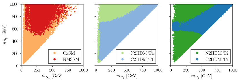
Figure 1: Masses of the two non-$h_{125}$ neutral scalars. Left: the CxSM (orange) and NMSSM (red); middle: the type I N2HDM (fair-green) and C2HDM (fair-blue); right: the type II N2HDM (dark-green) and C2HDM (dark-blue). For the CxSM, NMSSM and N2HDM the two masses in the axes are for CP-even Higgs bosons, whereas for the C2HDM they are for CP-mixed Higgs bosons . By definition $m_{H_{\downarrow}}\leq m_{H_{\uparrow}}$.

In all models we find points with $m_{H_{\downarrow}}<m_{h_{125}}$. For the C2HDM type II, however, this is only the case in the limit of the real 2HDM. Away from this limit the masses of $H_{\downarrow}$ and $H_{\uparrow}$ turn out to be always heavier than about 500 GeV and to be close. We have verified that this results from a combination of the tree-level unitarity constraints with the electroweak precision data constraints (through the $S,T,U$ variables). To conclude this, first we performed several scans, one for each constraint with only that constraint applied, to check the individual effect of each constraint. Then we repeated the procedure for all possible pairings of constraints. The upper boundary of the C2HDM mass spectra observed in the middle and right panels is the same for both types and it matches the one for the real 2HDM. This boundary is due to tree-level unitarity constraints. In the N2HDM there is more freedom, with further quartic couplings involving the singlet, so the same boundary does not arise.

In the N2HDM, the CxSM and C2HDM type I, we have points where $m_{H^{\uparrow}}<m_{h_{125}}$ and hence the $h_{125}$ is the heaviest of the CP-even (CP-mixed in the C2HDM) neutral Higgs bosons. In our scan, we did not find such points for the NMSSM. The N2HDM and NMSSM feature additionally pseudoscalars that can also be lighter than 125 GeV. The N2HDM covers the largest mass region. With the largest number of parameters, not restricted by additional supersymmetric symmetries, it is easiest in this model to adjust it to be compatible with all the applied constraints. Note, finally, that the gaps at 125 GeV are due to the mass windows around $h_{125}$ in order to avoid degenerate Higgs signals.

4.2 Phenomenology of the Singlet or Pseudoscalar Admixture in $h_{125}$

We investigate the phenomenology of the $h_{125}$ with respect to its possible singlet or pseudoscalar admixture. In particular, we study to which extent this influences the signal strengths of the $h_{125}$ and if this can be used to distinguish between the models. Additionally, we compare the CP-conserving singlet admixture with the CP-violating pseudoscalar admixture. Since the measurement of CP violation is experimentally very challenging, a $h_{125}$ of the C2HDM could be misidentified as a CP-even Higgs boson in the present phase of the LHC. Moreover, since the Higgs couplings to gauge bosons have the same Lorentz structure as the SM Higgs boson, a clear signal of CP violation would have to be seen either via the couplings to fermions or via particular combinations of decays if other Higgs were discovered [10]. A comparison of the singlet and pseudoscalar admixture is therefore appropriate.

In the CxSM, the singlet admixture to a Higgs boson $H_{i}$ is given by the sum of the real and complex singlet parts squared, i.e.

$$\Sigma_{i}^{\text{CxSM}}=(R_{i2})^{2}+(R_{i3})^{2}\;,$$ (4.146)

with the matrix $R$ defined in Eq. (2.11). In the N2HDM, the singlet admixture is given by

$$\Sigma_{i}^{\text{N2HDM}}=(R_{i3})^{2}\;,$$ (4.147)

where $R$ has been introduced in Eq. (2.102). Also in the NMSSM the singlet admixture is obtained from the square of the ’$i3$’ element of the mixing matrix,

$$\Sigma_{i}^{\text{NMSSM}}=({\cal R}^{S}_{i3})^{2}\;,$$ (4.148)

with ${\cal R}^{S}$ introduced in Eq. (2.115). Note, that we use the mixing matrix including higher order corrections as obtained from NMSSMTools. Finally, the pseudoscalar admixture $\Psi$ of the C2HDM is defined as

$$\Psi_{i}^{\text{C2HDM}}=(R_{i3})^{2}\;,$$ (4.149)

with $R$ introduced in Eq. (2.55). In the following we drop the subscript and denote by $\Sigma$ and $\Psi$ the singlet and pseudoscalar admixture of $h_{125}$, respectively.

The CxSM: In the CxSM the rescaling of all couplings to the SM particles by one common factor makes an agreement of large singlet admixtures with the experimental data impossible. The maximum allowed singlet admixture in the CxSM is given by the lower bound on the global signal strength $\mu$ and amounts to

$$\Sigma_{\text{max}}^{\text{CxSM}}\approx 1-\mu_{\text{min}}\approx 11\%\;.$$ (4.150)

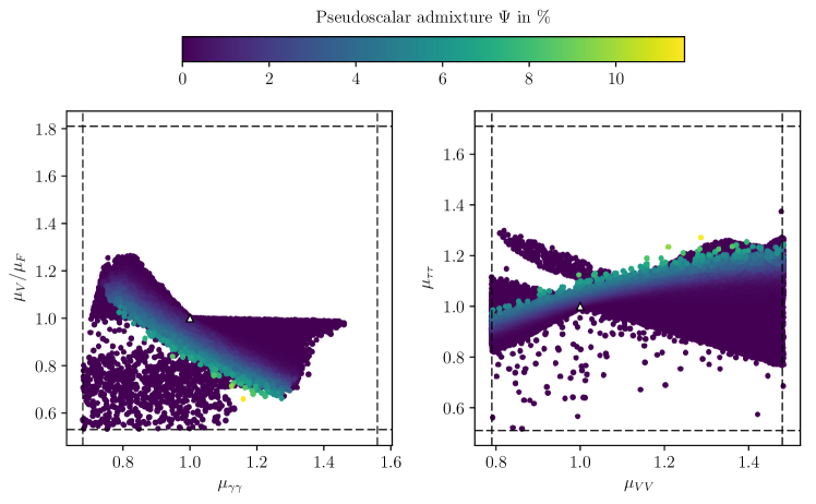
Figure 2: C2HDM type II: Pseudoscalar admixture $\Psi^{\text{C2HDM}}$ of $h_{125}$ as a function of the most constraining signal strengths. The dashed lines show the experimental limits and the white triangle denotes the SM value.

The C2HDM: We next discuss the pseudoscalar admixture in the C2HDM. Some features are also found in the N2HDM, so that we do not need to repeat in detail the discussion of the N2HDM, for which we refer to [33]. We start with the C2HDM type II. As can be inferred from Fig. 2, which shows the pseudoscalar admixture of the C2HDM SM-like Higgs boson as a function of the most constraining signal strengths, the pseudoscalar admixture can at most be 10%. This is not a consequence of the measured properties of the $h_{125}$ but due to the restrictive bounds on the electron EDM. Without EDM constraints 20% would be allowed. Because of the rather small $\Psi$, the properties of the $h_{125}$ in the C2HDM are well approximated by the real 2HDM. In this limit, there are only two non-zero mixing matrix elements that contribute to $h_{125}$. The orthogonality of the mixing matrix leads to the sharp edges of the allowed regions visible in the plots. In Fig. 2 we observe three regions of enhanced $\mu_{\tau\tau}$ in case of small pseudoscalar admixture (dark blue points). One of the dark blue enhanced regions resides in the wrong-sign limit and corresponds to the points deviating from the bulk (towards the top left in the right and towards the bottom left in the left plot of Fig. 2). Additionally, enhanced $\mu_{\tau\tau}$ rates can be observed for non-vanishing larger pseudoscalar admixture. This behaviour can be understood by investigating the couplings to gauge bosons and fermions individually. In Fig. 3 (left) $c^{2}(h_{125}VV)$ is plotted against $c^{2}(h_{125}b\bar{b})\equiv(c^{e})^{2}+(c^{o})^{2}$, with $c^{e,o}$ defined in Eq. (2.78). Note that in the 2HDM type II the tree-level couplings to down-type quarks and leptons are the same. The right figure shows $c^{2}(h_{125}t\bar{t})$ versus $c^{2}(h_{125}b\bar{b})$. The colour code indicates the pseudoscalar admixture.

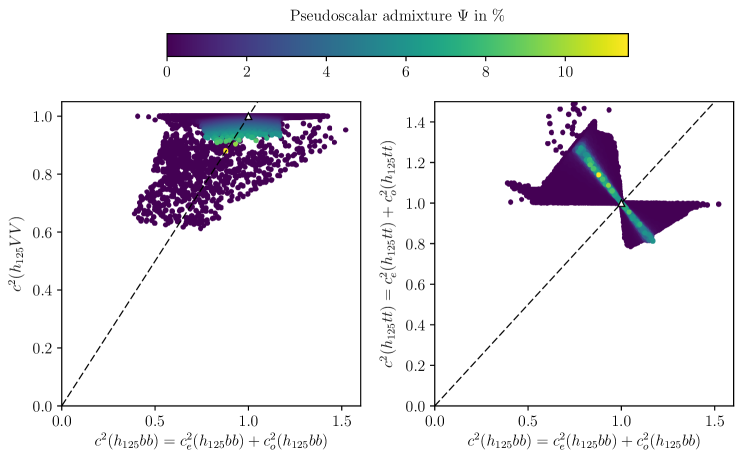
Figure 3: C2HDM type II: Pseudoscalar admixture $\Psi^{\text{C2HDM}}$ of $h_{125}$ as a function of the effective couplings squared. The white triangle denotes the SM value. The dashed line represents equal scaling of the couplings.

While the pseudoscalar admixture reduces the couplings to gauge bosons the couplings to fermions can be reduced or enhanced irrespective of the value of $\Psi$. The enhanced rates are due to enhanced couplings to top-quarks, thus increasing the production cross section. The additional reduction in $c(h_{125}VV)^{2}=\mu_{V}$ leads to the reduced $\mu_{V}/\mu_{F}$, observed for the points with larger pseudoscalar admixture in Fig. 2 (left). Here we also see points with strongly reduced $\mu_{V}/\mu_{F}$ and vanishing pseudoscalar admixture. As mentioned above, these are points residing either in the wrong-sign regime with strongly reduced couplings to the massive gauge bosons or in the region where substantial Higgs-to-Higgs decays of the $h_{125}$ are possible. They are almost exclusively points of the real 2HDM. The most enhanced $\mu_{\tau\tau}$ of up to 30% is obtained for simultaneously enhanced $\mu_{VV}$. It is due to the enhanced production mechanism resulting from enhanced couplings to the top quarks in this region, as we explicitly verified, while the involved decays remain SM-like. The second enhanced region in the CP-conserving limit, the one in the wrong sign regime, is due to reduced couplings to gauge bosons and simultaneously enhanced couplings to bottom quarks. The resulting reduced decay into $VV$ increases the branching ratio into $\tau\tau$ and thus the rate in this final state. The third region with enhanced $\mu_{\tau\tau}$ and reduced $\mu_{VV}$ arises from enhanced effective couplings to $\tau$ leptons and $b$-quarks. Combining this with the fact that the couplings to massive gauge bosons cannot exceed one, the overall branching ratio into $\tau$ pairs is enhanced.

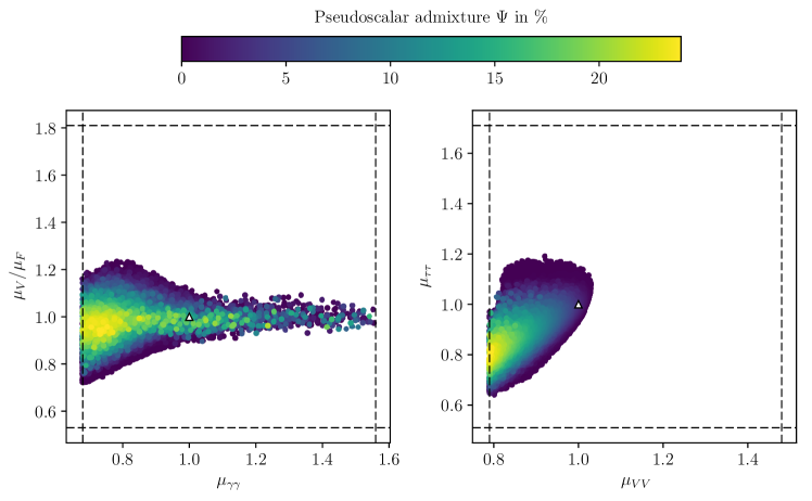
Figure 4: C2HDM type I: Pseudoscalar admixture $\Psi^{\text{C2HDM}}$ of $h_{125}$ as a function of the most constraining signal strengths. The dashed lines show the experimental limits and the white triangle denotes the SM value.

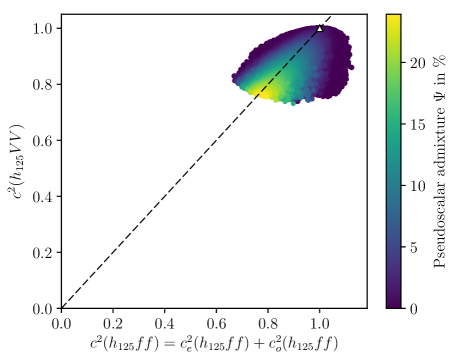
Figure 5: C2HDM type I: Pseudoscalar admixture $\Psi^{\text{C2HDM}}$ of $h_{125}$ as a function of the effective couplings squared. The white triangle denotes the SM value. The dashed line represents equal scaling of the couplings.

With values of up to 25%, cf. Fig. 4, larger pseudoscalar admixtures are allowed in the C2HDM type I compared to the type II. This upper bound of $\Psi$ is barely affected by the EDMs which are less constraining in the type I model. As can be inferred from Fig. 4, the upper bound of $\mu_{VV}$ as well as the boundaries of $\mu_{\tau\tau}$ and $\mu_{V}/\mu_{F}$ obtained from the combination of all the constraints in our scan are already well inside the upper bound restrictions set by the LHC data on these signal rates. In contrast to type II no enhanced rates can be observed for non-vanishing pseudoscalar admixture. The highest pseudoscalar admixtures entail reduced signal strengths, while simultaneously the ratio $\mu_{V}/\mu_{F}\approx 1$. In Fig. 5 $c^{2}(h_{125}VV)$ is plotted against $c^{2}(h_{125}t\bar{t})=c^{2}(h_{125}b\bar{b})$. The colour code shows that both effective couplings are reduced almost in parallel with increasing $\Psi$, implying $\mu_{V}/\mu_{F}\approx 1$ for large pseudoscalar admixture. We find that for a measurement of $\mu_{\tau\tau}$ within 5% of the SM value pseudoscalar admixtures above 15% are excluded. If $\mu_{VV}$ is determined within 5% of the SM value, $\Psi$ is even constrained to values below 7%. In type II, only a simultaneous measurement of all $\mu$ values within 5% of their SM values constrain $\Psi$ to below about 3%.

The N2HDM: In the N2HDM, the large number of free parameters allows for significant non-SM properties of the $h_{125}$. We have investigated the singlet admixture of the SM-like N2HDM Higgs boson in great detail in [33] and found that in the N2HDM type II singlet admixtures of up to 55% are still compatible with the LHC Higgs data. Interestingly, the most constraining power on $\Sigma^{\text{N2HDM}}$ does not arise from the best measured signal rates $\mu_{VV}$ and $\mu_{\gamma\gamma}$ which for SM-like rates in these channels still allow for singlet admixtures of up to 50% and 40%, respectively. However, a measurement of $\mu_{\tau\tau}\approx 1$ constrains $\Sigma^{\text{N2HDM}}$ to values below about 25%, and $\mu_{V}/\mu_{F}\geq 1$ restrict it to below 20%. This can be understood by inspecting the involved couplings and is due to a stronger reduction of the coupling to bottom quarks with rising singlet admixture than the ones to top quarks and $VV$. For details, we refer the reader to [33]. Since the N2HDM and the C2HDM coincide in their scalar sector in the limit of vanishing singlet admixture and pseudoscalar admixture, respectively, we observe the same enhanced regions of $\mu_{\tau\tau}$ in the limit of the real 2HDM (type II). Away from this limit both models differ: While non-vanishing pseudoscalar admixture allows for enhanced $\mu_{\tau\tau}$, the singlet admixture in the N2HDM always reduces the rates, in contrast to the C2HDM case the couplings to fermions become smaller with rising $\Sigma$.

In the N2HDM type I due to the restriction of the up- and down-type quark couplings to the same doublet we found that the maximum allowed singlet admixture is 25%, inducing reduced signal strengths with simultaneously $\mu_{V}/\mu_{F}\approx 1$. The distribution of the couplings in the parameter space is similar to that of the C2HDM type I, cf. [33] for comparison. Like in the C2HDM type I, the singlet admixture is most effectively constrained, down to about 7.5%, by a 5% measurement of $\mu_{VV}$, while in type II $\mu_{\tau\tau}$ restricts $\Sigma$ to below 37% (20%) for small (medium) $\tan\beta$ values if it is measured to 5% within the SM value.

The NMSSM: Figure 6 displays the singlet admixture of the NMSSM SM-like Higgs boson as a function of the most constraining signal strengths. These are in the left plot $\mu_{V}/\mu_{F}$ versus $\mu_{\gamma\gamma}$ and $\mu_{\tau\tau}$ versus $\mu_{VV}$ in the right one. The colour code quantifies the singlet admixture. Due to the correlations enforced on the Higgs sector from supersymmetry, the NMSSM parameter space is much more constrained than the one of the N2HDM (cf. [33] for the corresponding plots of the N2HDM). Furthermore, $\mu_{\tau\tau}$ cannot be enhanced by more than a few percent, in contrast to the type II N2HDM, where enhancements of up to 40% are still compatible with the Higgs data. The reasons for possible (large) enhancement of $\mu_{\tau\tau}$ in the N2HDM (or C2HDM) are all absent in the NMSSM: In the NMSSM the effective coupling to top quarks cannot exceed 1, i.e.

$$c^{2}(h_{125}t\bar{t})\leq 1\;,$$ (4.151)

with $c(h_{125}t\bar{t})$ denoting the coupling modification factor with respect to the SM coupling. This can be inferred from Fig. 7, which shows the correlations between the NMSSM effective couplings squared together with the singlet admixture. In the N2HDM on the other hand, the squared top-Yukawa coupling, which controls the dominant gluon fusion production mechanism, can be enhanced by more than 60%. In the N2HDM the wrong-sign regime also allows for increased $\mu_{\tau\tau}$ whereas in the NMSSM we did not find such points. Finally, the $h_{125}$ coupling squared to bottom quarks can be enhanced by more than 40% in the N2HDM compared to only about 15% in the NMSSM, cf. Fig. 7.

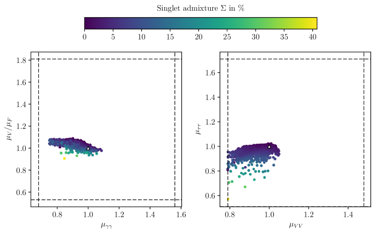
Figure 6: NMSSM: Singlet admixture $\Sigma^{\text{NMSSM}}$ of $h_{125}$ as a function of the most constraining signal strengths. The dashed lines show the experimental limits and the white triangle denotes the SM value.

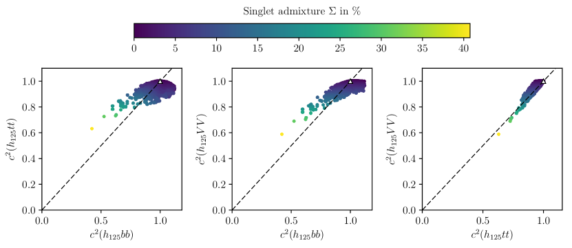
Figure 7: NMSSM: Singlet admixture $\Sigma^{\text{NMSSM}}$ of the $h_{125}$ as a function of the effective couplings squared. The white triangle denotes the SM value. The dashed lines represent equal scaling of the couplings.

While in the N2HDM the ratio $\mu_{V}/\mu_{F}$ reaches its lower experimental bound of 0.54 for $\mu_{\gamma\gamma}$ up to 1.2, cf. [33], in the NMSSM this ratio does not drop much below 1. The reason is the correlation

$$c^{2}(h_{125}t\bar{t})\approx c^{2}(h_{125}VV)\;,$$ (4.152)

increasing with rising singlet admixture, as can be inferred from Fig. 7 (right). The coupling to top quarks controls gluon fusion and thus $\mu_{F}$, while $c^{2}(h_{125}VV)\approx\mu_{V}$, so that $\mu_{V}\approx\mu_{F}$. This is a consequence of the SUSY relations together with the requirement of the $h_{125}$ to behave SM-like.

The NMSSM can still accommodate a considerable singlet admixture of up to $\Sigma^{\text{NMSSM}}=42$%. Like in the N2HDM, with rising $\Sigma$ the effective coupling squared $c^{2}(h_{125}b\bar{b})$ is reduced more strongly than $c^{2}(h_{125}VV)$ and $c^{2}(h_{125}t\bar{t})$, as can be inferred from Fig. 7 (left and middle). The enhancement in the branching ratios due to the reduced dominant decay into $b\bar{b}$ and hence the smaller total width is large enough to counterbalance the reduction in the production. The coupling strength to $\tau$’s is reduced in the same way as the one to bottom quarks when the singlet admixture increases. As there are no other means to enhance $\mu_{\tau\tau}$ in order to compensate for the effects of non-zero singlet admixture, the $\mu_{\tau\tau}$ is very constraining and even more constraining than in the N2HDM. A measurement of $\mu_{\tau\tau}$ within 5% of the SM value would exclude singlet admixtures larger than 8%.

5 Signal Rates of the non-SM-like Higgs Bosons

In this section we show and compare the rates of all neutral non-SM-like Higgs bosons in the most important SM final state channels. Assuming that in a first stage of discovery only one additional Higgs boson besides the $h_{125}$ has been discovered we also investigate the question if in this situation, i.e. before the discovery of further Higgs bosons, we are already able to distinguish between the four models discussed here. As the determination of the CP properties of the new Higgs boson is not immediate and takes some time to accumulate a sufficiently large amount of data, we assume that the CP properties of the second discovered Higgs boson are not known, so that we have to treat the CP-even, CP-odd and CP-mixed (in the C2HDM) Higgs bosons of our models on equal footing. Again, we denote by $H_{\downarrow}$ the lighter and by $H_{\uparrow}$ the heavier of the two neutral non-$h_{125}$ CP-even or CP-mixed (for the C2HDM) Higgs bosons. The pseudoscalar of the N2HDM is denoted by $A$ and the two pseudoscalars of the NMSSM by $A_{1}$ and $A_{2}$, where by definition $m_{A_{1}}<m_{A_{2}}$. The signal rates that we show have been obtained by multiplying the production cross section with the corresponding branching ratio obtained from sHDECAY, N2HDECAY, NMSSMCALC and a private version including the CP-violating 2HDM (to be published in a forthcoming paper). For the production we use

$$\sigma_{\Phi}=\sigma_{\Phi}(ggF)+\sigma_{\Phi}(bbF)\;,$$ (5.153)

computed for a c.m. energy of $\sqrt{s}=13$ TeV with SusHi at NNLO QCD using the effective $t$ and $b$ couplings of the respective model. Here $\Phi$ generically denotes any of the CP-even, CP-odd and CP-mixed neutral Higgs bosons of our models. Production through bottom-quark fusion is included in order to account for possible large $b$-quark couplings. None of our models can lead to enhanced couplings to vector bosons, so that we neglect the sub-leading production through vector boson fusion. As Higgs-strahlung and associated production are negligible compared to $ggF$ and $bbF$, we neglect these production channels as well. Furthermore, for all rates we impose a lower limit of 0.1 fb.

Signal Rates into $ZZ$: In Fig. 8 we depict the signal rates into $ZZ$. The rates of the two non-SM-like Higgs bosons of the C2HDM are shown together with the CP-even Higgs bosons of the other models in one plot, although they can have a more or less important pseudoscalar admixture. Note also, that there are no rates for the pure pseudoscalar Higgs bosons of the N2HDM and NMSSM, as they do not couple to massive gauge bosons at tree-level. For all our models the sum rule

$$\sum_{i=1}^{3}c^{2}(H_{i}VV)=1$$ (5.154)

for the CP-even and C2HDM CP-mixed Higgs bosons holds, imposed by unitarity constraints. Since the $h_{125}$ requires substantial couplings to gauge bosons in order to comply with the experimental results in the $ZZ$ and $W^{+}W^{-}$ final states, the sum rule forces the gauge coupling of $H_{\downarrow}$ (and also $H_{\uparrow}$) to be considerably below the SM value. The room for deviations of the $h_{125}$-Higgs boson coupling to gauge bosons from the SM value mainly depends on the number of free parameters of the model that can be used to accommodate independent coupling variations. This allows e.g. a reduction of the decay width into gauge bosons to be compensated by the reduction of the total width and/or an increase in the production cross section.

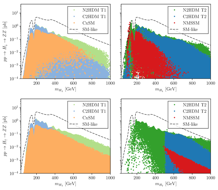
Figure 8: Signal rates for the production of $H_{\downarrow}$ (upper) and $H_{\uparrow}$ (lower) decaying into a pair of $Z$ bosons at the $\sqrt{s}=13$ TeV LHC as a function of its mass. Left: the CxSM (orange), the type I N2HDM (fair green) and C2HDM (fair blue). Right: the NMSSM (red) and the type II N2HDM (dark green) and C2HDM (dark blue). The dashed black line denotes the signal rate of a SM Higgs boson of the same mass.

In the CxSM the common scaling of all Higgs couplings combined with the sum rule Eq. (5.154) and the fact that experimental data allow for $\mu_{h_{125}}$ down to about 0.9 enforces

$$c^{2}_{\text{CxSM}}(H_{\downarrow/\uparrow}VV)\raisebox{-3.69899pt}{~{}\shortstack{$<$ \\ [-0.07cm] $\sim$}}~{}0.1\;.$$ (5.155)

As all CxSM Higgs couplings are reduced compared to the SM the production cross sections cannot be enhanced in this model, so that altogether not only the rate into $VV$ but all CxSM rates are below the SM reference in the whole $m_{H_{\downarrow/\uparrow}}$ mass range so that the discovery of additional Higgs bosons in the CxSM may proceed through Higgs-to-Higgs decays [12].

Also for the remaining models overall we observe reduced rates compared to what would be expected in the SM for a Higgs boson of the same mass, except for the low-mass region. The resulting rates are a combination of sum rules and the behaviour of the Yukawa couplings. As the $h_{125}$ takes a large portion of the coupling to gauge bosons, the $H_{\downarrow/\uparrow}VV$ coupling necessarily cannot be substantial. Models with more parameters, however, like the ones discussed here, allow for larger deviations of the $h_{125}$ couplings from the SM expectations. This allows the remaining Higgs bosons to have larger couplings, while maintaining compatibility with any coupling sum rules. We will discuss the implications of such sum rules in great detail in the next section. As we have seen before the couplings to fermions can also be enhanced in some models. Finally, due to SUSY relations the NMSSM has less freedom than the N2HDM. Overall the combination of all these effects leads to the rates in most mass regions being largest in the N2HDM. Furthermore, the rates in the type I models are (somewhat) smaller than in the corresponding type II models, as in the former we have the additional constraint that the up- and down-type couplings cannot be varied independently.

The behaviour of the NMSSM cross sections can be best understood by looking at the nature of the Higgs boson under investigation. This is summarized in Table 2 of Ref. [9]. The $H_{\downarrow}$ with mass below 125 GeV behaves singlet-like but can become doublet-like in regions with strong doublet-singlet mixing which happens in mass regions close to 125 GeV. This is why here the rates can become SM-like or even exceed the SM reference value. In this case, where the second-lightest Higgs $H_{2}\equiv h_{125}$, the heaviest one, $H_{\uparrow}$, is doublet-like. In case the lightest Higgs boson $H_{1}\equiv h_{125}$, $H_{\downarrow}$ is singlet (doublet)-like for small (large) $\tan\beta$, and $H_{\uparrow}$ takes the opposite role. Despite the fact that for masses above 125 GeV either $H_{\downarrow}$ or $H_{\uparrow}$ are doublet-like their couplings to massive gauge bosons are suppressed as discussed in [9] so that the NMSSM rates always remain well below the SM reference.

Since all the rates of the various models overlap, a distinction based on this criterion is difficult. One can state, however, that an observation of a neutral scalar with an ${\cal O}(100\mbox{ fb})$ rate in the $ZZ$ channel for a mass $\raisebox{-3.69899pt}{~{}\shortstack{$>$ \\ [-0.07cm] $\sim$}}~{}380$ GeV may be sufficient to exclude the NMSSM. Furthermore the observation of rates of 30-50 fb in the high mass region between 800 and 1000 GeV can only be due to the N2HDM (type II), within our set of models. This region is being tested by the experiments, which are due to achieve soon the luminosity necessary to probe such high rates [119].

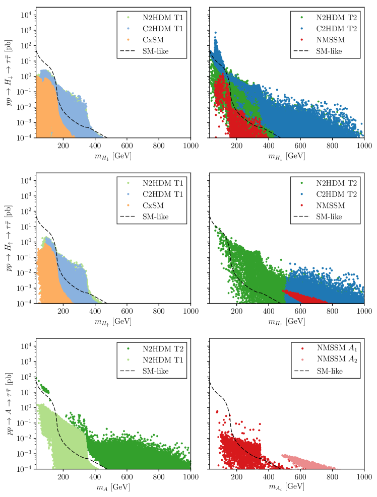
Figure 9: Same as Fig. 8 but for the $\tau$-pair final state. Also included, in the lower row: tauonic decays of the N2HDM pseudoscalar $A$ (left) for the types I (fair green) and II (dark green) and of the NMSSM pseudoscalars (right) $A_{1}$ (red) and $A_{2}$ (rose).

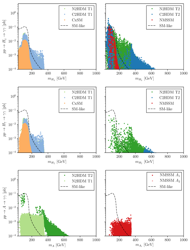
Figure 10: Same as Fig. 9 but for the photonic final state.

Signal Rates into $\tau\tau$: Figure 9 displays the signal rates into the $\tau$-pair final state for the various models. In all models apart from the CxSM the $H_{\downarrow/\uparrow}$ couplings to $\tau$-pairs can be enhanced above the SM value, so that enhanced rates are possible provided the production cross section is not too strongly suppressed. In particular in the C2HDM, the incoherent addition of the scalar and pseudoscalar contributions to both the $ggF/bbF$ production and the partial width into $\tau\bar{\tau}$ leads to enhanced rates. This concerns the points with non-vanishing $\Psi$ where $m_{H_{\uparrow/\downarrow}}\raisebox{-3.69899pt}{~{}\shortstack{$>$ \\ [-0.07cm] $\sim$}}~{}500$ GeV. All other points reside in the limit of the CP-conserving 2HDM, as discussed above. Note that the points of the type II N2HDM and C2HDM (here in the $\Psi\to 0$ limit) with enhanced $\tau$ rates for $m_{H_{\downarrow}}\raisebox{-3.69899pt}{~{}\shortstack{$<$ \\ [-0.07cm] $\sim$}}~{}200$ GeV are about to be constrained (or excluded) experimentally [120]. The very enhanced points at $m_{H_{\downarrow}}=70-80$ GeV are due to associated production with bottom quarks for large values of $\tan\beta$ in the real 2HDM limit of both the C2HDM and N2HDM. In this mass region no exclusion limits exist so far so that these points are still allowed. This should encourage the experiments to perform analyses in this mass region. For $m_{H_{\downarrow}}\raisebox{-3.69899pt}{~{}\shortstack{$<$ \\ [-0.07cm] $\sim$}}~{}65$ GeV, limits exist from the SM-like Higgs data, as $h_{125}$ can decay off-shell into a pair of $H_{\downarrow}$ which could possibly spoil the measured $\mu$-values of $h_{125}$. The NMSSM rates are explained as follows: Irrespective of $\tan\beta$ the $H_{\downarrow}$ is singlet-like for $m_{H_{\downarrow}}<125$ GeV and becomes more and more doublet-like in the vicinity of $h_{125}$ so that its rates become more SM-like. For $m_{H_{\downarrow}}\geq 130$ GeV $H_{\downarrow}$ is singlet-(doublet-)like for small (large) $\tan\beta$. The applied limits on the SUSY masses turn out to restrict the NMSSM parameter range to smaller values of $\tan\beta$, so that $H_{\downarrow}$ is singlet-like in this mass region and its rates are below the SM reference values. The $H_{\uparrow}$ is doublet-like for $\tan\beta$ small and $h_{125}$ either $H_{1}$ or $H_{2}$. As $\tan\beta$ cannot become large, however, its rates are not much above the values that would be obtained in the SM case.

The lower two plots display the production cross sections of the N2HDM pseudoscalar $A$ in the N2HDM (left plot) and of the two NMSSM pseudoscalars $A_{1}$ and $A_{2}$. The SM-like Higgs limit is also included in the dashed line as a reference. Again in N2HDM type II the rates are larger than in type I. In the range $130\mbox{ GeV}\leq m_{A}\raisebox{-3.69899pt}{~{}\shortstack{$<$ \\ [-0.07cm] $\sim$}}~{}200$ GeV there are hardly any points due to the LHC exclusion limits [120]. The enhanced rates for $m_{A}\leq 120$ GeV are on the border of being excluded. The shape of the NMSSM $A_{1,2}$ distributions is again explained by the singlet-/ doublet-nature of these particles. The lighter of the two pseudoscalars, $A_{1}$, is singlet-like for $m_{A_{1}}\raisebox{-3.69899pt}{~{}\shortstack{$<$ \\ [-0.07cm] $\sim$}}~{}380$ GeV. Still, in the region above the $Z$-pair and below the top-quark pair threshold, the $\tau\tau$ rates can exceed the SM reference, as the decay into $ZZ$ bosons which is dominant here in the SM, is absent. The sharp edge at 350 GeV is due to the opening of the decay into top-quarks. The $A_{2}$ is correspondingly doublet-, i.e. MSSM-like, explaining its larger rates for the same mass value.

The comparison of all models shows that it is impossible to distinguish the models based on these rates. Only the CxSM can be excluded if rates above the SM are found, as expected.

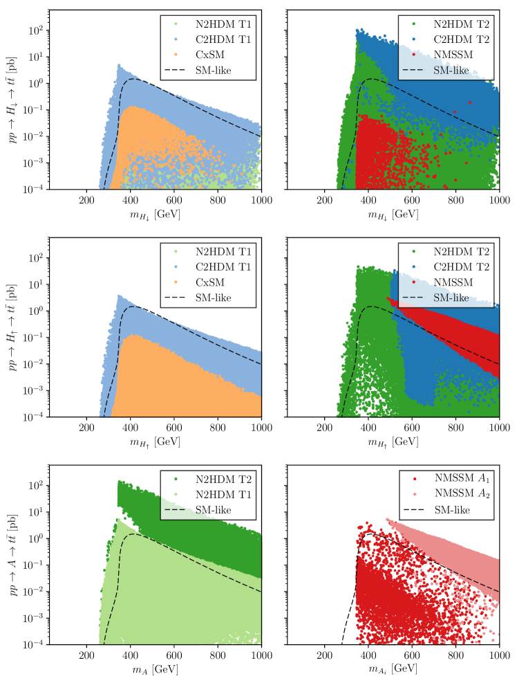
Figure 11: Same as Fig. 9 but for the top-quark pair final state.

Signal rates into $\gamma\gamma$: In Fig. 10 we study the rates in the photonic final state. The distributions show the same shape as for the tauonic final state, only moved downwards to smaller rates. Interesting are the enhanced photonic rates for mass values below 125 GeV in the upper right plot for the NMSSM and the type II N2HDM and C2HDM. The latter, however, are points in the limit of the real 2HDM. The N2HDM points are hidden behind the NMSSM ones and reach equally large rates. The even higher 2HDM points will soon be constrained (or excluded) once the experimental analyses investigate this mass range. These findings, however, should further encourage searches in these mass regions in the tauonic and photonic final states. Also in the photonic final state, the distinction of the model based on the final states is difficult. Only the observation of rates above 5 fb in the mass range between 130 and 350 GeV would indicate a (non-supersymmetric) extended Higgs sector of type II Yukawa structure as the only valid model among the ones we are discussing. However, these rates are experimentally challenging.

Signal rates into $tt$: Finally, in Fig. 11 the rates into top-quark pair final states are shown. The largest rates are achieved in the type II N2HDM and C2HDM, where the C2HDM points cover the N2HDM points, which reach equally high rates. Note, however, that again all points below 500 GeV are only obtained in the limit of the real 2HDM and not related to any CP-mixing. The NMSSM $H_{\downarrow}$ rates are far below the SM ones, as $H_{\downarrow}$ is singlet-like for small values $\tan\beta$. It behaves doublet-like for large values of $\tan\beta$. But then the decay into tops is suppressed. However, the $H_{\uparrow}$ is doublet-like for small $\tan\beta$ values inducing rates above the SM ones. Also the NMSSM pseudoscalar $A_{2}$ is doublet-like for small $\tan\beta$ values, so that large rates are obtained, while $A_{1}$ is doublet-like for large $\tan\beta$, so that large rates are precluded. In the N2HDM type II small values of $\tan\beta$ are still allowed so that large rates can be obtained for $A$, which couples proportionally to $1/\tan\beta$ to up-type quarks both in type I and II. With rates of up to ${\cal O}(100\mbox{ fb})$ and more, the search for heavy (pseudo)scalars in the top-pair final state in the 2HDM, N2DHM and NMSSM becomes interesting. A distinction of the models is difficult. The NMSSM, however, can be excluded if rates above 20 fb are observed in the top-pair final state.

6 Coupling Sums

In this section we investigate what can be learnt about the underlying model from the coupling patterns of the discovered Higgs bosons. We study the gauge boson sum

$$\Pi^{(i)}_{VV}=\sum_{j=1}^{i}|c(H_{j}VV)|^{2}$$ (6.156)

and the Yukawa sum

$$\Pi^{(i)}_{\text{Yuk}}=\frac{1}{\sum_{j=1}^{i}|c(H_{i}\tau\bar{\tau})|^{2}}+\frac{1}{\sum_{j=1}^{i}|c(H_{i}t\bar{t})|^{2}}\;.$$ (6.157)

As evident from these definitions

$$\Pi^{(i)}_{VV}\leq\Pi^{(i+1)}_{VV}\quad\mbox{and}\quad\Pi^{(i)}_{\text{Yuk}}\geq\Pi^{(i+1)}_{\text{Yuk}}\;.$$ (6.158)

The sums are performed over the CP-even Higgs bosons of the CxSM, N2HDM and NMSSM, and over the CP-violating neutral Higgs bosons of the C2HDM. In the C2HDM and the N2HDM, the Yukawa sum depends on the way the Higgs doublets couple to the fermions. In type II, the coupling to $\tau$ leptons can be exchanged by the $b$-quarks, leading to the same result, which for the sum over all neutral Higgs bosons is independent of $\tan\beta$. In the remaining types, this Yukawa sum can be dependent on $\tan\beta$. In our analysis we assume the experimental situation that only one additional neutral Higgs boson with non-vanishing gauge coupling has been discovered.

Note that for the unitarity of scattering processes to be fulfilled the couplings of the Higgs bosons to the gauge bosons and to the fermions, respectively, have to take a specific form. All our models are weakly interacting, and the couplings fulfil the unitarity requirement, expressed through sum rules [121, 122, 123]. The specific form of the coupling sum rules can be derived from 2-to-2 scattering processes, by requiring these to fulfil unitarity. Thus, longitudinal gauge boson scattering into a pair of longitudinal gauge bosons implies that $\Pi^{(i)}_{VV}$ is equal to 1 if the sum is performed over all Higgs bosons coupling to the gauge bosons. If one Higgs boson is missed the sum rule is violated. The sum over the fermion couplings has not been derived from a 2-to-2 scattering process. Instead it has been constructed such that it yields 1 for the NMSSM and the type II N2HDM when the complete sum over all CP-even Higgs bosons is performed. The outcome of the Yukawa sum defined in Eq. (6.158) depends on the way the Higgs doublets couple to the fermions, so that the sums for the N2HDM type I and the C2HDM type I and II depend on the model parameter $\tan\beta$. In the following we will investigate how the gauge boson and Yukawa sums in our models change if the sum is performed only over a subset of the Higgs bosons. In case not all neutral Higgs bosons of a given model are included in the gauge boson sum, it will deviate from 1. In the MSSM and the CP-conserving 2HDM, however, the sum over two discovered CP-even Higgs bosons is complete and yields 1 both for the gauge boson sum rule and the Yukawa sum (2HDM type II only).

At the LHC the Higgs couplings can only be extracted by applying model assumptions. The accuracy at 68% C.L. on the $VV$ and $\tau\tau$ couplings to be expected for an integrated luminosity of 300 fb^-1 (3000 fb^-1) is about 10% (slightly better than 10%), on the $t$-quark coupling about 15% ($\sim$12%) and around 20% (16%) for the $b$-quark coupling, see e.g. [124, 125, 126, 127]. The model-independent coupling measurements at a linear collider (LC) improve these precisions to a few percent at a c.m. energy of 500 GeV with an integrated luminosity of 500 fb^-1 [127, 128, 129, 130, 131, 132]. The combination of the high-luminosity LHC and LC leads to a further improvement on the extracted accuracy. Due to the lower statistics the precision on the Higgs couplings of the non-SM-like Higgs bosons might be somewhat lower. Their CP-even or -odd nature can be tested in an earlier stage after discovery by applying different spin-parity hypotheses. The measurement of possibly CP-violating admixtures, however, requires the accumulation of a large amount of data, so that a dominantly CP-even Higgs boson of the C2HDM can be misinterpreted as CP-even and is taken into account in this analysis, as also argued above.

In the C2HDM and CxSM all three neutral Higgs bosons mix so that the coupling sum analysis can straightforwardly be applied. For the N2HDM and NMSSM, however, it has to be made sure that the additionally discovered Higgs boson included in the sum, is CP-even. If the observed particle is observed in the $ZZ$ decay channel, it cannot be purely CP-odd [133, 134, 10]. Therefore, we require for the non-SM-like Higgs boson

$$ggF\to H_{\downarrow/\uparrow}\to ZZ>10\mbox{ fb}\;.$$ (6.159)

This should be observable at the high-luminosity LHC, especially if properties of the particle are known from prior observations in other channels. This still allows for $H_{\downarrow/\uparrow}$ to be a CP-mixed state, which leads to interesting phenomenological consequences for the C2HDM. In [135, 136, 137] it has been shown that the loop-induced decay $A\to ZZ$ of the pure pseudoscalar in the CP-conserving 2HDM can lead to considerable rates. Assuming that a similar behaviour might be possible in the N2HDM, the $ZZ$ decay channel might not be sufficient to unambiguously identify the CP nature of the Higgs boson, but other measurements like e.g. the angular distributions in $Z$- and $\gamma$-pair final states or fermionic decay modes could be used to identify the CP nature of the discovered particle, see e.g. [138, 139, 140, 141, 142, 143, 144, 133, 145], and to ensure no CP-odd particle is included in the sum.

With the coupling sums at hand, we want to investigate the following questions in the next three subsections:

• Assuming that only two neutral CP-even (or, for the C2HDM, two dominantly CP-even) Higgs bosons have been found, can we decide based on the coupling sums if the CP-even (or, for the C2HDM, CP-mixed) Higgs sector is complete (like e.g. in the MSSM or CP-conserving 2HDM that incorporate only two CP-even Higgs bosons) or if we are missing the discovery of the remaining Higgs bosons of an extended Higgs sector?

• If this is possible, does the inspection of the pattern of the coupling sums allow us to draw conclusions on the mass scale of the missing Higgs boson?

• Furthermore, can we distinguish between the various models investigated here on the basis of the sum distributions of the two discovered Higgs bosons?

6.1 Gauge Boson Coupling Sums

For all of our models we have

$$\Pi^{(3)}_{VV}=1\quad\mbox{ for the CxSM, N2HDM, NMSSM, C2HDM}\;,$$ (6.160)

whereas in models with smaller Higgs sectors as the CP-conserving 2HDM or the MSSM, the gauge boson sum reads

$$\Pi^{(2)}_{VV}=1\quad\mbox{ for the MSSM and the CP-conserving 2HDM}\;.$$ (6.161)

Figure 12 shows the distribution of the partial gauge boson sum $\Pi^{(2)}_{VV}$ for our models. We assume that besides $h_{125}$ only one additional CP-even (or, for the C2HDM, CP-mixed) Higgs boson has been discovered. In this case, the sum rule Eq. (6.160) is necessarily violated, as we only sum over two instead of three Higgs bosons, and we expect to see deviations of $\Pi^{(2)}_{VV}$ from 1. In the left column, we assume that the additionally discovered Higgs boson is the $H_{\downarrow}$, and in the right one, it is assumed to be the $H_{\uparrow}$. Without the discovery of the third Higgs boson, we cannot decide in which of the two situations we are. The upper (lower) row shows the distributions as a function of the (non-)discovered Higgs boson mass, respectively. All the points that are shown respect all our constraints, including the requirement of Eq. (6.159).

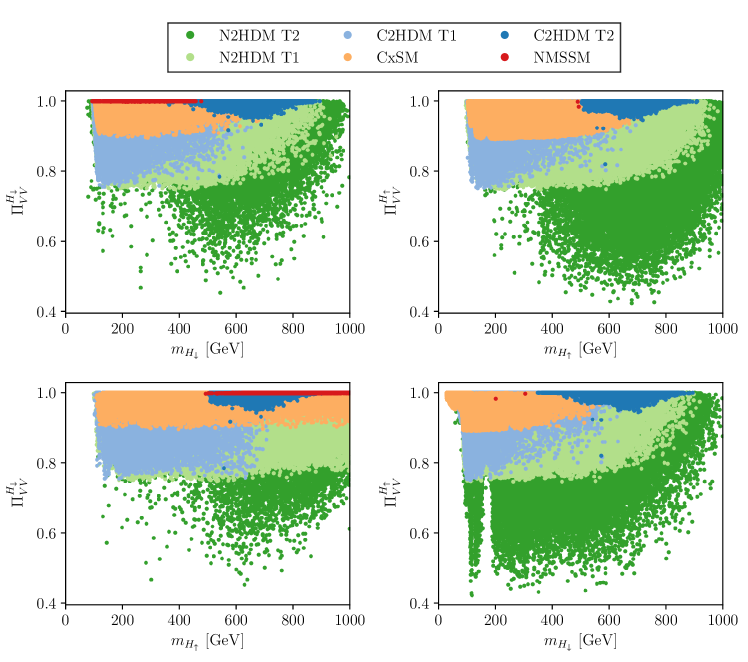
Figure 12: The partial gauge boson sum $\Pi^{(2)}_{VV}$ assuming the only additionally discovered Higgs boson is $H_{\downarrow}$ (left) or $H_{\uparrow}$ (right) as a function of their respective mass (upper) and as a function of the mass of the non-discovered Higgs boson, respectively, (lower), for the CxSM (yellow), the type I N2HDM (fair green) and C2DHM (fair blue), the type II N2HDM (dark green) and C2HDM (dark blue) and the NMSSM (red).

We immediately observe, that $\Pi^{(2)}_{VV}$ cannot drop below about 0.9 in the CxSM. This is a consequence of the simple coupling structure combined with the bound from the global signal strength, enforcing $c^{2}(h_{125}VV)\raisebox{-3.69899pt}{~{}\shortstack{$>$ \\ [-0.07cm] $\sim$}}~{}0.9$ or equivalently $\Pi^{(2)}_{VV}\raisebox{-3.69899pt}{~{}\shortstack{$>$ \\ [-0.07cm] $\sim$}}~{}0.9$, even if the discovered non-SM Higgs does not couple to $VV$. Hence, deviations by more than 0.1 from the total gauge boson sum would allow to exclude the CxSM, although it is more likely that the CxSM can be excluded by deviations from the common coupling scaling, before the coupling sum analysis can be performed.

In the C2HDM type II, apart from very few outliers, the $h_{125}$ coupling squared to massive gauge bosons can deviate by at most 10% from the squared SM-value, cf. Fig. 3, which is reflected in the outcome of the gauge coupling sum shown here. In the C2HDM type I on the other hand larger deviations from the SM-limit are still possible, cf. Fig. 5, so that the partial gauge coupling sum can become as small as 0.73.

In the N2HDM type II (type I) deviations from 1 of up to 55% (25%) in $c^{2}(h_{125}VV)$ are possible, inducing the largest deviations of all models from $\Pi_{VV}=1$. They are also larger than those attained by the outliers in C2HDM type II. Moreover, the few outliers in the C2HDM that can reach a violation of 35% are likely to be probed before a coupling sum analysis can be performed. The NMSSM, on the other hand, although featuring the largest Higgs sector, is the most constrained of our models because of supersymmetric relations. As a consequence, the coupling sum can deviate by at most a few percent if the second discovered Higgs boson is $H_{\downarrow}$. In case it is the heavier one, we hardly have any points that fulfil the requirement of rates above 10 fb in the $Z$ boson final state, cf. Fig. 8. In this case, the coupling sum deviates a bit more from 1, by up to about 5%.

In summary, the answers to our questions are, that all models feature points where the gauge coupling sum is very close to 1 or equal to 1 making it very hard to distinguish them from the real 2HDM or the MSSM. This is not surprising as all our models contain the alignment limit, cf. also [146]. On the other hand, in all our models there exist parameter configurations (although very rare for the NMSSM and the C2HDM type II) where considerable deviations from 1 allow for an easy discrimination from the Higgs sectors with two neutral Higgs bosons. The coupling sum analysis allows for the exclusion of the CxSM if $\Pi^{(2)}_{VV}$ deviates by more than 10% from 1, while in the C2HDM it would indicate the realization of the wrong-sign regime. As the lower plots reveal, a correlation between the pattern of the coupling sum and the mass scale of the escaped Higgs boson cannot be observed after taking into account all mentioned constraints. Finally, the observation of deviations by more than 35% singles out the N2HDM as a possible underlying model.

6.2 Yukawa Coupling Sums

The CxSM fulfils the Yukawa coupling sum

$$\Pi^{(3)}_{\text{Yuk}}=2\;.$$ (6.162)

In the NMSSM and in the type II (as well as the lepton-specific) N2HDM we have

$$\Pi^{(3)}_{\text{Yuk}}=1\;.$$ (6.163)

The flipped N2HDM implies the same coupling sum if the $\tau$-lepton coupling is exchanged by the $b$-quark coupling. For the C2HDM Yukawa sum we use the effective fermion coupling squared $|c(Hf\bar{f})|^{2}\equiv(c^{e})^{2}+(c^{o})^{2}$, with $c^{e}$ and $c^{o}$ defined in Eq. (2.78). For the C2HDM type II this leads to the sum

$$\Pi^{(3)}_{\text{Yuk}}=2\left(\frac{24}{17-\cos(4\beta)}-1\right)\;.$$ (6.164)

The Yukawa sum as a function of $\tan\beta$ is shown in Fig. 13 (short-dashed blue line). It has a minimum of $\Pi^{(3)}_{\text{Yuk}}=2/3$ at $\tan\beta=1$ and quickly approaches 1 from below for all other $\tan\beta$ values.

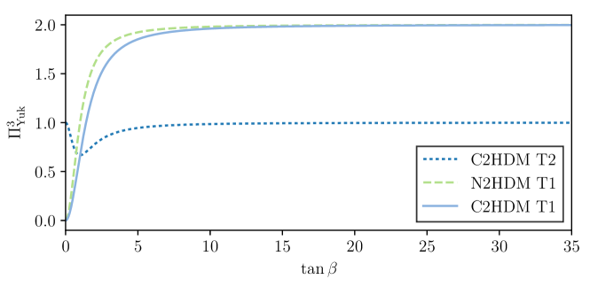
Figure 13: The non-trivial Yukawa sums for the C2HDM type II (short-dashed blue), Eq. (6.164), the N2HDM type I (dashed green), Eq. (6.165) and the C2HDM type I (full blue), Eq. (6.166), as a function of $\tan\beta$.

In type I, the Yukawa sum is the same both for the $\tau$-lepton and the $b$-quark choice of the down-type fermion coupling. In the N2HDM type I, we have

$$\Pi^{(3)}_{\text{Yuk}}=2\sin^{2}\beta\;,$$ (6.165)

and in the C2HDM type I the sum reads

$$\Pi^{(3)}_{\text{Yuk}}=\frac{2\tan^{2}\beta}{2+\tan^{2}\beta}.$$ (6.166)

Both of these are also shown in Fig. 13 (dashed green and full blue line, respectively). Flavour constraints [75, 76] require $\tan\beta\geq 2.2$ in type I models which means that $\Pi^{(3)}_{\mathrm{Yuk}}$ cannot be much smaller than 2 (cf. Fig. 13) in both the C2HDM and N2HDM type I. The result for the sums is the same in the flipped type, and also in the lepton-specific case if the $b$-quark is used instead of the $\tau$-lepton. For the real 2HDM (MSSM) the Yukawa sums are the same as in the N2HDM (NMSSM) with the difference that one only sums over 2 instead of 3 neutral Higgs bosons.

In Fig. 14 the distributions of the partial Yukawa sums $\Pi^{(2)}_{\rm Yuk}$ are depicted for the two situations where the additionally discovered CP-even (or, for the C2HDM, CP-mixed) Higgs boson is either the lighter (left column) or the heavier (right column) of the non-SM Higgs bosons. The upper (lower) row again shows the distributions as a function of the (non-)discovered Higgs boson mass, respectively.

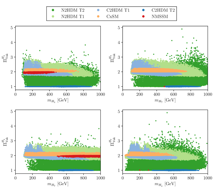
Figure 14: Same as Fig. 12 but for the partial Yukawa sum $\Pi^{(2)}_{\text{Yuk}}$.

We observe, that due to the common rescaling of all CxSM Higgs couplings the lower bound of the partial Yukawa sum is given by 2 with the maximal violation of the complete sum given by the bound of the global signal strength. The measurement of a value below 2 would immediately exclude the CxSM. A measurement of $\Pi^{(2)}_{\text{Yuk}}<1$ on the other hand, would be very interesting because it is only possible in the C2HDM type II and due to the specific pseudoscalar admixture to the Yukawa couplings. Therefore, not only the model but also the structure of the Yukawa sector could be determined. According to Eq. (6.164) it would also fix $\tan\beta\approx 1$. Since the deviations from 1 can at most be a few percent, however, the model is most probably identified earlier through other observables. The C2HDM type II is ruled out if deviations larger than $7$% above 1 are measured. In the C2HDM type I the values of the partial Yukawa sum are distributed between about 1.7 and 2.8. The lower limit is due to the lower bound on $\tan\beta$ imposed by the flavour constraints. The observation of any violation below 1.7 and above about 2.8 immediately excludes the C2HDM type I. This also applies for the N2HDM type I where the maximum deviations range between the partial sum values 1.7 and 2.8.

In the NMSSM the partial Yukawa sum is strongly violated with values between 1.8 and 2 if the additional discovered Higgs boson is the lighter one. If instead $H_{\uparrow}$ is discovered the Yukawa sum is close to the saturating value of 1. These two very different violation patterns allow to decide which of the two non-SM-like Higgs bosons has been discovered, if one is able to identify the NMSSM as the underlying model. The NMSSM is excluded if violations beyond 2 are discovered. The large violations in case $H_{\downarrow}$ is discovered can be explained by the fact that the constraints applied on the NMSSM restrict $\tan\beta$ to small values. For these, however, the heavier CP-even Higgs boson $H_{\uparrow}$ is dominantly doublet-like, cf. Table 2 in [9]. While $h_{125}$ carries most of the top-Yukawa coupling to comply with the Higgs data, the non-discovered doublet-like $H_{\uparrow}$ has a large coupling component to the down-type fermions. Its non-discovery leads to the observed large violations in $\Pi^{(2)}_{\text{Yuk}}$. The situation is reversed if $H_{\uparrow}$ is discovered. The $H_{\downarrow}$ is mostly singlet-like and its non-discovery barely violates the Yukawa sum, which is close to 1. Finally, the N2HDM type II with its large number of parameters not restricted by SUSY relations can violate the Yukawa sum by a factor of almost 5. Any measurement of $\Pi^{(2)}_{\text{Yuk}}$ beyond about 2.9 therefore clearly singles out the N2HDM type II among our candidate models.

In summary, the answers to our questions are: The type I C2HDM and N2HDM, the type II N2HDM, the CxSM and the NMSSM all feature points around the value $2\sin^{2}\beta$, that is obtained for the sum of the 2HDM type I, so that a distinction from this model would then not be possible. However, if the two discovered Higgs bosons are those of the type I C2HDM or N2HDM, the CxSM or the two lighter Higgs bosons of the NMSSM, then their sum would clearly exclude the possibility of the 2DHM type II or the MSSM, as these lead to the sum value of 1. The scale of the non-discovered Higgs boson cannot be determined from the pattern of the Yukawa coupling sums. Only in the NMSSM coupling sums close to 1 would indicate that the discovered Higgs boson is the $H_{\uparrow}$, and above 1.8, that it is the $H_{\downarrow}$. The distinction of the models, or at least the exclusion of some of the models is possible as described in the previous paragraph.

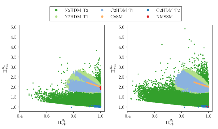
Figure 15: Partial Yukawa sum $\Pi^{(2)}_{\text{Yuk}}$ versus $\Pi^{(2)}_{VV}$ in case $H_{\downarrow}$ (left) or $H_{\uparrow}$ (right) has been discovered.

6.3 Coupling Sum Correlations

The previous discussions have already made clear that there are correlations between the gauge boson and Yukawa coupling sums that may be exploited. In Fig. 15 the partial sums are plotted against each other for all of our models and the two different discovery situations. The CxSM shows the simplest behaviour where the two sums are strongly correlated due to the common rescaling of the couplings. As also all other models except for the C2HDM type II cover (part of) this region this behaviour does not allow to distinguish the models. Only deviations from this correlation rule out the CxSM. In the NMSSM the plot clearly shows the two distinct regions resulting from the discovery of either the $H_{\downarrow}$ or the $H_{\uparrow}$. However, it is impossible in both regions to distinguish the NMSSM from the other models using only these coupling sums. The N2HDM is by far the least constrained of our models. It shows a sharp lower boundary which is a result of the orthogonality of the mixing matrix and not due to the physical constraints. Observing $\Pi^{(2)}_{VV}<1$ and $\Pi^{(2)}_{\text{Yuk}}\approx 1$ therefore excludes all models with a $3\times 3$ mixing of the CP-even scalars. The other models do not have any points in this region because of their specific Yukawa structure and/or the influence of other constraints. The only model in our study where such a situation could be realized is the C2HDM type II, identifying it as the candidate underlying model in this case.

7 Conclusions

In this paper we investigated extensions of the SM, that are motivated by specific features. Namely, they may solve some of the problems of the SM, they are rather simple, and they feature 3 CP-even Higgs bosons that have a singlet admixture. These are the CxSM, the N2HDM and the NMSSM. Additionally, we included the C2HDM as it also provides 3 neutral Higgs bosons, which, however, now have a pseudoscalar admixture. This allows us to compare the phenomenological implications of the different admixtures. Furthermore, all these models are based on different underlying symmetries that, again, are reflected in the phenomenology of their Higgs bosons. In view of the non-discovery of new non-SM particles, we investigated what can be learnt from the Higgs sector itself. Our main focus was on the experimental situation where besides the discovered SM-like Higgs boson only one additional Higgs is discovered in a first stage. We considered the question: Can the different models be distinguished based on the mass distributions, the discovery rates as well as the gauge boson and Yukawa coupling sums? Independently of this goal, the rates of all neutral Higgs bosons for the investigated models in the various SM final states presented here can be used as basis for further investigations, like e.g. the identification of benchmark points. Note that all generated parameter points fulfil the experimental and theoretical constraints on the models. Our main findings are the following:

The EDM constraints, that are relevant for the CP-violating 2HDM, turn out to be more constraining in the C2HDM type II than in type I. For a non-negligible CP-violating phase, the Higgs mass spectrum is characterized by rather heavy non-SM-like Higgs bosons, with both masses above about 500 GeV and not too far apart.

While either of the two lighter CP-even (CP-mixed in case of the C2HDM) Higgs bosons can be the SM-like Higgs in our models, the mass spectrum of the NMSSM and C2HDM type II does not feature the possibility of the heaviest Higgs boson to be the SM-like one.

We found that the present constraints all allow for a non-vanishing singlet or pseudoscalar admixture to the $h_{125}$ that, depending on the model, is more or less important and can be constrained by future measurements of the rates. The results are summarized in table 4. The N2HDM results are taken from [33]. Note that the upper bound on $\Psi$ for the C2HDM type II is mainly due to the EDM constraints. We also found that the C2HDM type II is the only model where $\mu_{\tau\tau}$ increases with rising value of the admixture.

Model	CxSM	C2HDM II	C2HDM I	N2HDM II	N2HDM I	NMSSM
$\left(\Sigma\,{\rm or}\,\Psi\right)_{\text{allowed}}$	11%	10%	20%	55%	25%	41%
$\mu_{x}(\left(\Sigma\,{\rm or}\,\Psi\right)_{\text{max}})$	global	all (7.5%)	$\mu_{VV}$ (7% )	$\mu_{\tau\tau}$ (20-37%)	$\mu_{VV}$ (7.5%)	$\mu_{\tau\tau}$ (8%)

Table 4: 2nd row: allowed singlet and pseudoscalar (for the C2HDM) admixtures; 3rd row: the most constraining $\mu_{xx}$ together with the maximum allowed admixture after a measurement of $\mu_{xx}$ within 5% of the SM value. The allowed CxSM admixture scales with the global signal strength. The first (second) value for N2HDM II applies for medium (small) $\tan\beta$ values.

From the investigation of the rates of the non-SM-like Higgs bosons, which can be CP-even, CP-odd or CP-mixed states we concluded, regarding the observation of one additional neutral Higgs boson $\Phi$ besides the $h_{125}$, that:

• The CxSM is excluded in any of the SM final state channels if rates above the SM reference are found.

• In the $ZZ$ final state, rates of ${\cal O}(100)$ fb for $m_{\Phi}\raisebox{-3.69899pt}{~{}\shortstack{$>$ \\ [-0.07cm] $\sim$}}~{}380$ GeV exclude the NMSSM, and rates of 35-50 fb for $m_{\Phi}\in[800:1000]$ GeV are only possible in the N2HDM II. The latter rates are about to be probed by the experiments, however.

• In the $\tau\tau$ final state, we find strongly enhanced rates for the C2HDM and N2HDM type II in the limit of the real 2HDM for $m_{\Phi}\in\left[70:80\right]$ GeV. This is also the case for the pseudoscalar decay in the N2HDM type II. This should encourage the experiments to extend their analyses to this mass range. Overall, no distinction of the models is possible based on this final state rate alone.

• In the $\gamma\gamma$ final state, we find again strongly enhanced rates for $m_{\Phi}\in[70:80]$ GeV in the C2HDM for $\Psi\to 0$, as the experiments have not provided exclusion limits here yet. Furthermore, rates above 5 fb for $m_{\Phi}\in[130:350]$ GeV single out the N2HDM II as the only allowed model in our set.

• In the $t\bar{t}$ final state the N2HDM, C2HDM and NMSSM rates can be above the SM reference and even reach ${\cal O}(100)$ pb in the N2HDM rendering the search for the additional Higgs bosons in this final state interesting. Note that the NMSSM is found to be excluded if rates above about 4 pb are measured.

The requirement of unitarity implies coupling sum rules. In case not all the Higgs bosons that carry an electroweak doublet component are found, these sum rules are violated. This gives a handle to decide whether the discovered Higgs spectrum is complete or not. Thus, we investigated the partial gauge boson and Yukawa sums assuming that only one additional Higgs boson besides the $h_{125}$ has been discovered. In our models with three CP-even (CP-mixed, for the C2HDM) Higgs bosons this inevitably induces violations of the coupling sums. We found, for all our models, that the partial gauge boson sum contains points where the sum rule is fulfilled. This is to be expected, as the $h_{125}$ couples almost SM-like to the massive gauge bosons. In this case, a distinction from the MSSM or the 2HDM with two CP-even Higgs bosons is impossible. Also in the partial Yukawa sums we found scenarios fulfilling the complete sum. There are a lot of scenarios, however, that violate the complete coupling sums and that can be used to identify some distinguishing features:

• The violation of the gauge boson sum rule by more than 10% excludes the CxSM, the violation by more than 35% singles out the N2HDM as a candidate underlying model. In case the NMSSM can be identified as the underlying model, by finding e.g. additional supersymmetric particles, the violation of the sum rule would allow it to be distinguished from the MSSM, for which the sum rule is saturated after the discovery of two CP-even Higgs bosons. Measurable violations of the gauge boson sum rule are, however, only observed if the additionally discovered Higgs bosons is the $H_{\uparrow}$ and if $H_{\downarrow}$ has a mass near 125 GeV.

• The violation of the Yukawa sum with values below 2 excludes the CxSM and with values above 2 the NMSSM. In case the partial Yukawa sum yields values below 1, the candidate model is the C2HDM II. The C2HDM II on the other hand is excluded for values above 1.07. If the partial sum yields values below 1.7 or above 2.85 then the type I C2HDM or N2HDM are excluded. If it is a supersymmetric model and deviations by more than 80% away from 1 are observed, then the candidate is the NMSSM and, in that case, the $H_{\downarrow}$ has been discovered. For values close to 1 it is the $H_{\uparrow}$ that has been discovered. Finally, values above 2.9 for the partial Yukawa sum single out the N2HDM II as the candidate underlying model.

Our results show, that even if only a subset of the Higgs bosons of extended Higgs sectors is found, the use of the Higgs rates and coupling sums and their combination may allow for the distinction of models and eventually even for the identification of a specific candidate model. The next step to be taken now is the definition of benchmark points that feature specific properties to support this task and that the experiments can include in their experimental analyses.

Acknowledgements

The authors acknowledge financial support from the DAAD project “PPP Portugal 2015” (ID: 57128671) and from the FCT project “Exploring Beyond the Standard Model Higgs Sectors”. M.S. is funded through the grant BPD/UI97/5528/2017. The work in this paper was also supported by the CIDMA project UID/MAT/04106/2013. We would like to thank Philipp Basler, Rohini Godbole and Michael Spira for useful discussions.

References

- [1] G. Aad et al. [ATLAS Collaboration], Phys.Lett. B716, 1 (2012), 1207.7214.
- [2] S. Chatrchyan et al. [CMS Collaboration], Phys.Lett. B716, 30 (2012), 1207.7235.
- [3] C. Englert et al., J. Phys. G41, 113001 (2014), 1403.7191.
- [4] V. Khachatryan et al. [CMS Collaboration], Phys. Rev. D92, 012004 (2015), 1411.3441.
- [5] G. Aad et al. [ATLAS Collaboration], Eur. Phys. J. C75, 476 (2015), 1506.05669.
- [6] V. Khachatryan et al. [CMS Collaboration], Eur. Phys. J. C75, 212 (2015), 1412.8662.
- [7] G. Aad et al. [ATLAS Collaboration], Eur. Phys. J. C76, 6 (2016), 1507.04548.
- [8] G. Aad et al. [ATLAS and CMS Collaboration], Phys. Rev. Lett. 114, 191803 (2015), 1503.07589.
- [9] S. F. King, M. Muhlleitner, R. Nevzorov, and K. Walz, Phys. Rev. D90, 095014 (2014), 1408.1120.
- [10] D. Fontes, J. C. Romao, R. Santos, and J. P. Silva, Phys. Rev. D92, 055014 (2015), 1506.06755.
- [11] S. F. King, M. Muhlleitner, R. Nevzorov, and K. Walz, Nucl. Phys. B901, 526 (2015), 1508.03255.
- [12] R. Costa, M. Muhlleitner, M. O. P. Sampaio, and R. Santos, JHEP 06, 034 (2016), 1512.05355.
- [13] R. S. Gupta, H. Rzehak, and J. D. Wells, Phys. Rev. D86, 095001 (2012), 1206.3560.
- [14] R. S. Gupta, H. Rzehak, and J. D. Wells, Phys. Rev. D88, 055024 (2013), 1305.6397.
- [15] R. Grober, M. Muhlleitner, and M. Spira, JHEP 06, 080 (2016), 1602.05851.
- [16] R. Coimbra, M. O. P. Sampaio, and R. Santos, Eur. Phys. J. C73, 2428 (2013), 1301.2599.
- [17] J. F. Gunion, H. E. Haber, G. L. Kane, and S. Dawson, Front.Phys. 80, 1 (2000).
- [18] T. D. Lee, Phys. Rev. D8, 1226 (1973).
- [19] G. C. Branco et al., Phys. Rept. 516, 1 (2012), 1106.0034.
- [20] X.-G. He, T. Li, X.-Q. Li, J. Tandean, and H.-C. Tsai, Phys. Rev. D79, 023521 (2009), 0811.0658.
- [21] B. Grzadkowski and P. Osland, Phys. Rev. D82, 125026 (2010), 0910.4068.
- [22] H. E. Logan, Phys. Rev. D83, 035022 (2011), 1010.4214.
- [23] M. S. Boucenna and S. Profumo, Phys. Rev. D84, 055011 (2011), 1106.3368.
- [24] X.-G. He, B. Ren, and J. Tandean, Phys. Rev. D85, 093019 (2012), 1112.6364.
- [25] Y. Bai, V. Barger, L. L. Everett, and G. Shaughnessy, Phys. Rev. D88, 015008 (2013), 1212.5604.
- [26] X.-G. He and J. Tandean, Phys. Rev. D88, 013020 (2013), 1304.6058.
- [27] Y. Cai and T. Li, Phys. Rev. D88, 115004 (2013), 1308.5346.
- [28] L. Wang and X.-F. Han, Phys. Lett. B739, 416 (2014), 1406.3598.
- [29] A. Drozd, B. Grzadkowski, J. F. Gunion, and Y. Jiang, JHEP 11, 105 (2014), 1408.2106.
- [30] R. Campbell, S. Godfrey, H. E. Logan, A. D. Peterson, and A. Poulin, Phys. Rev. D92, 055031 (2015), 1505.01793.
- [31] S. von Buddenbrock et al., Eur. Phys. J. C76, 10 (2016), 1606.01674.
- [32] C.-Y. Chen, M. Freid, and M. Sher, Phys. Rev. D89, 075009 (2014), 1312.3949.
- [33] M. Muhlleitner, M. O. P. Sampaio, R. Santos, and J. Wittbrodt, (2016), 1612.01309.
- [34] P. Fayet, Nucl.Phys. B90, 104 (1975).
- [35] R. Barbieri, S. Ferrara, and C. A. Savoy, Phys.Lett. B119, 343 (1982).
- [36] M. Dine, W. Fischler, and M. Srednicki, Phys.Lett. B104, 199 (1981).
- [37] H. P. Nilles, M. Srednicki, and D. Wyler, Phys.Lett. B120, 346 (1983).
- [38] J. Frere, D. Jones, and S. Raby, Nucl.Phys. B222, 11 (1983).
- [39] J. Derendinger and C. A. Savoy, Nucl.Phys. B237, 307 (1984).
- [40] J. R. Ellis, J. Gunion, H. E. Haber, L. Roszkowski, and F. Zwirner, Phys.Rev. D39, 844 (1989).
- [41] M. Drees, Int.J.Mod.Phys. A4, 3635 (1989).
- [42] U. Ellwanger, M. Rausch de Traubenberg, and C. A. Savoy, Phys.Lett. B315, 331 (1993), hep-ph/9307322.
- [43] U. Ellwanger, M. Rausch de Traubenberg, and C. A. Savoy, Z.Phys. C67, 665 (1995), hep-ph/9502206.
- [44] U. Ellwanger, M. Rausch de Traubenberg, and C. A. Savoy, Nucl.Phys. B492, 21 (1997), hep-ph/9611251.
- [45] T. Elliott, S. King, and P. White, Phys.Lett. B351, 213 (1995), hep-ph/9406303.
- [46] S. King and P. White, Phys.Rev. D52, 4183 (1995), hep-ph/9505326.
- [47] F. Franke and H. Fraas, Int.J.Mod.Phys. A12, 479 (1997), hep-ph/9512366.
- [48] M. Maniatis, Int.J.Mod.Phys. A25, 3505 (2010), 0906.0777.
- [49] U. Ellwanger, C. Hugonie, and A. M. Teixeira, Phys.Rept. 496, 1 (2010), 0910.1785.
- [50] I. F. Ginzburg, M. Krawczyk, and P. Osland, Two Higgs doublet models with CP violation, in Linear colliders. Proceedings, International Workshop on physics and experiments with future electron-positron linear colliders, LCWS 2002, Seogwipo, Jeju Island, Korea, August 26-30, 2002, pp. 703–706, 2002, hep-ph/0211371.
- [51] W. Khater and P. Osland, Nucl. Phys. B661, 209 (2003), hep-ph/0302004.
- [52] A. W. El Kaffas, W. Khater, O. M. Ogreid, and P. Osland, Nucl. Phys. B775, 45 (2007), hep-ph/0605142.
- [53] A. W. El Kaffas, P. Osland, and O. M. Ogreid, Nonlin. Phenom. Complex Syst. 10, 347 (2007), hep-ph/0702097.
- [54] A. Wahab El Kaffas, P. Osland, and O. M. Ogreid, Phys. Rev. D76, 095001 (2007), 0706.2997.
- [55] P. Osland, P. N. Pandita, and L. Selbuz, Phys. Rev. D78, 015003 (2008), 0802.0060.
- [56] A. Arhrib, E. Christova, H. Eberl, and E. Ginina, JHEP 04, 089 (2011), 1011.6560.
- [57] A. Barroso, P. M. Ferreira, R. Santos, and J. P. Silva, Phys. Rev. D86, 015022 (2012), 1205.4247.
- [58] D. Fontes, J. C. Romao, and J. P. Silva, JHEP 12, 043 (2014), 1408.2534.
- [59] S. P. Martin, Adv.Ser.Direct.High Energy Phys. 21, 1 (2010), hep-ph/9709356.
- [60] S. Dawson, p. 261 (1997), hep-ph/9712464.
- [61] A. Djouadi, Phys.Rept. 459, 1 (2008), hep-ph/0503173.
- [62] R. Costa, R. Guedes, M. O. P. Sampaio, and R. Santos, ScannerS project, 2014, http://scanners.hepforge.org.
- [63] A. Djouadi, J. Kalinowski, and M. Spira, Comput. Phys. Commun. 108, 56 (1998), hep-ph/9704448.
- [64] J. M. Butterworth et al., The Tools and Monte Carlo Working Group Summary Report from the Les Houches 2009 Workshop on TeV Colliders, in Physics at TeV colliders. Proceedings, 6th Workshop, dedicated to Thomas Binoth, Les Houches, France, June 8-26, 2009, 2010, 1003.1643.
- [65] L. Lavoura and J. P. Silva, Phys. Rev. D50, 4619 (1994), hep-ph/9404276.
- [66] F. J. Botella and J. P. Silva, Phys. Rev. D51, 3870 (1995), hep-ph/9411288.
- [67] M. E. Peskin and T. Takeuchi, Phys. Rev. D46, 381 (1992).
- [68] I. Maksymyk, C. Burgess, and D. London, Phys.Rev. D50, 529 (1994), hep-ph/9306267.
- [69] R. Costa, A. P. Morais, M. O. P. Sampaio, and R. Santos, Phys. Rev. D92, 025024 (2015), 1411.4048.
- [70] P. Bechtle et al., Eur. Phys. J. C74, 2693 (2014), 1311.0055.
- [71] G. Aad et al. [ATLAS and CMS Collaboration], JHEP 08, 045 (2016), 1606.02266.
- [72] I. P. Ivanov and J. P. Silva, Phys. Rev. D92, 055017 (2015), 1507.05100.
- [73] H. E. Haber and H. E. Logan, Phys. Rev. D62, 015011 (2000), hep-ph/9909335.
- [74] O. Deschamps et al., Phys. Rev. D82, 073012 (2010), 0907.5135.
- [75] F. Mahmoudi and O. Stal, Phys. Rev. D81, 035016 (2010), 0907.1791.
- [76] T. Hermann, M. Misiak, and M. Steinhauser, JHEP 11, 036 (2012), 1208.2788.
- [77] M. Misiak et al., Phys. Rev. Lett. 114, 221801 (2015), 1503.01789.
- [78] M. Misiak and M. Steinhauser, (2017), 1702.04571.
- [79] Gfitter Group, M. Baak et al., Eur. Phys. J. C74, 3046 (2014), 1407.3792.
- [80] The ATLAS collaboration, ATLAS-CONF-2016-073 (2016)
- [81] R. V. Harlander, S. Liebler, and H. Mantler, Comput. Phys. Commun. 184, 1605 (2013), 1212.3249.
- [82] R. V. Harlander, S. Liebler, and H. Mantler, Comput. Phys. Commun. C212, 239 (2017), 1605.03190.
- [83] P. Hafliger and M. Spira, Nucl. Phys. B719, 35 (2005), hep-ph/0501164.
- [84] S. Inoue, M. J. Ramsey-Musolf, and Y. Zhang, Phys. Rev. D89, 115023 (2014), 1403.4257.
- [85] ACME, J. Baron et al., Science 343, 269 (2014), 1310.7534.
- [86] T. Abe, J. Hisano, T. Kitahara, and K. Tobioka, JHEP 01, 106 (2014), 1311.4704, [Erratum: JHEP04,161(2016)].
- [87] W. Grimus, L. Lavoura, O. M. Ogreid, and P. Osland, J. Phys. G35, 075001 (2008), 0711.4022.
- [88] W. Grimus, L. Lavoura, O. M. Ogreid, and P. Osland, Nucl. Phys. B801, 81 (2008), 0802.4353.
- [89] U. Ellwanger, J. F. Gunion, and C. Hugonie, JHEP 02, 066 (2005), hep-ph/0406215.
- [90] U. Ellwanger and C. Hugonie, Comput. Phys. Commun. 175, 290 (2006), hep-ph/0508022.
- [91] U. Ellwanger and C. Hugonie, Comput. Phys. Commun. 177, 399 (2007), hep-ph/0612134.
- [92] D. Das, U. Ellwanger, and A. M. Teixeira, Comput. Phys. Commun. 183, 774 (2012), 1106.5633.
- [93] M. Muhlleitner, A. Djouadi, and Y. Mambrini, Comput. Phys. Commun. 168, 46 (2005), hep-ph/0311167.
- [94] G. Belanger, F. Boudjema, C. Hugonie, A. Pukhov, and A. Semenov, JCAP 0509, 001 (2005), hep-ph/0505142.
- [95] J. Baglio et al., Comput. Phys. Commun. 185, 3372 (2014), 1312.4788.
- [96] Planck, P. A. R. Ade et al., Astron. Astrophys. 571, A16 (2014), 1303.5076.
- [97] D. S. Akerib et al. [LUX Collaboration], Phys. Rev. Lett. 118, 021303 (2017), 1608.07648.
- [98] M. Spira, (1995), hep-ph/9510347.
- [99] P. M. Ferreira, R. Guedes, M. O. P. Sampaio, and R. Santos, JHEP 12, 067 (2014), 1409.6723.
- [100] The ATLAS collaboration, ATLAS-CONF-2013-090.
- [101] The CMS Collaboration, CMS-PAS-HIG-12-052.
- [102] G. Aad et al. [ATLAS Collaboration], JHEP 1510 (2015) 054, arXiv:1507.05525.
- [103] M. Aaboud et al. [ATLAS Collaboration], Phys. Rev. D 94 (2016) no.5, 052009, arXiv:1606.03903.
- [104] M. Aaboud et al. [ATLAS Collaboration], Eur. Phys. J. C 76 (2016) no.10, 547, arXiv:1606.08772.
- [105] M. Muhlleitner and E. Popenda, JHEP 1104 (2011) 095, arXiv:1102.5712.
- [106] R. Gröber, M. M. Mühlleitner, E. Popenda and A. Wlotzka, Eur. Phys. J. C 75 (2015) 420, arXiv:1408.4662.
- [107] R. Gröber, M. Mühlleitner, E. Popenda and A. Wlotzka, Phys. Lett. B 747 (2015) 144, arXiv:1502.05935.
- [108] G. Aad et al. [ATLAS Collaboration], Eur. Phys. J. C 75 (2015) no.10, 510 Erratum: [Eur. Phys. J. C 76 (2016) no.3, 153, arXiv:1506.08616.
- [109] M. Aaboud et al. [ATLAS Collaboration], Phys. Rev. D 94 (2016) no.3, 032005, arXiv:1604.07773.
- [110] G. Aad et al. [ATLAS Collaboration], JHEP 1405 (2014) 071, arXiv:1403.5294.
- [111] G. Aad et al. [ATLAS Collaboration], Eur. Phys. J. C 75 (2015) no.5, 208, arXiv:1501.07110.
- [112] F. Domingo and G. Weiglein, JHEP 1604 (2016) 095.
- [113] M. Carena, H. E. Haber, I. Low, N. R. Shah and C. E. M. Wagner, Phys. Rev. D 93 (2016) no.3, 035013.
- [114] V. Khachatryan et al. [CMS Collaboration], Phys. Lett. B 759 (2016) 672, arXiv:1602.04305.
- [115] G. Aad et al. [ATLAS Collaboration], Eur. Phys. J. C 76 (2016) no.12, 658, arXiv:1602.04516.
- [116] M. Muhlleitner, J. C. Romão, R. Santos, J. P. Silva, and J. Wittbrodt, to appear.
- [117] P. M. Ferreira, J. F. Gunion, H. E. Haber and R. Santos, Phys. Rev. D 89 (2014) no.11, 115003.
- [118] S. F. King, M. Muhlleitner, R. Nevzorov, and K. Walz, Nucl. Phys. B870, 323 (2013), 1211.5074.
- [119] The CMS Collaboration, CMS-PAS-HIG-16-034.
- [120] The ATLAS Collaboration, ATLAS-CONF-2016-085; The CMS Collaboration, CMS-PAS-HIG-16-037.
- [121] J. M. Cornwall, D. N. Levin, and G. Tiktopoulos, Phys. Rev. D10, 1145 (1974), [Erratum: Phys. Rev.D11,972(1975)].
- [122] J. F. Gunion, H. E. Haber, and J. Wudka, Phys. Rev. D43, 904 (1991).
- [123] B. Grzadkowski, J. F. Gunion, and J. Kalinowski, Phys. Rev. D60, 075011 (1999), hep-ph/9902308.
- [124] R. Lafaye, T. Plehn, M. Rauch, D. Zerwas, and M. Duhrssen, JHEP 08, 009 (2009), 0904.3866.
- [125] M. Klute, R. Lafaye, T. Plehn, M. Rauch, and D. Zerwas, Phys. Rev. Lett. 109, 101801 (2012), 1205.2699.
- [126] T. Plehn and M. Rauch, Europhys. Lett. 100, 11002 (2012), 1207.6108.
- [127] P. Bechtle, S. Heinemeyer, O. Stal, T. Stefaniak, and G. Weiglein, JHEP 11, 039 (2014), 1403.1582.
- [128] M. Klute, R. Lafaye, T. Plehn, M. Rauch, and D. Zerwas, Europhys. Lett. 101, 51001 (2013), 1301.1322.
- [129] ECFA/DESY LC Physics Working Group, J. A. Aguilar-Saavedra et al., (2001), hep-ph/0106315.
- [130] CLIC Physics Working Group, E. Accomando et al., Physics at the CLIC multi-TeV linear collider, in Proceedings, 11th International Conference on Hadron spectroscopy (Hadron 2005): Rio de Janeiro, Brazil, August 21-26, 2005, 2004, hep-ph/0412251.
- [131] ILC, G. Aarons et al., (2007), 0709.1893.
- [132] H. Baer et al., (2013), 1306.6352.
- [133] LHC Higgs Cross Section Working Group, J. R. Andersen et al., (2013), 1307.1347.
- [134] LHC Higgs Cross Section Working Group, D. de Florian et al., (2016), 1610.07922.
- [135] A. Arhrib and R. Benbrik, (2006), hep-ph/0610184.
- [136] W. Bernreuther, P. Gonzalez, and M. Wiebusch, Eur. Phys. J. C69, 31 (2010), 1003.5585.
- [137] J. L. Diaz-Cruz, C. G. Honorato, J. A. Orduz-Ducuara, and M. A. Perez, Phys. Rev. D90, 095019 (2014), 1403.7541.
- [138] S. Y. Choi, D. J. Miller, M. M. Muhlleitner, and P. M. Zerwas, Phys. Lett. B553, 61 (2003), hep-ph/0210077.
- [139] D. J. Miller, S. Y. Choi, B. Eberle, M. M. Muhlleitner, and P. M. Zerwas, Phys. Lett. B505, 149 (2001), hep-ph/0102023.
- [140] R. M. Godbole, D. J. Miller, and M. M. Muhlleitner, JHEP 12, 031 (2007), 0708.0458.
- [141] S. Berge, W. Bernreuther, and J. Ziethe, Phys. Rev. Lett. 100, 171605 (2008), 0801.2297.
- [142] S. Berge and W. Bernreuther, Phys. Lett. B671, 470 (2009), 0812.1910.
- [143] S. Berge, W. Bernreuther, B. Niepelt, and H. Spiesberger, Phys. Rev. D84, 116003 (2011), 1108.0670.
- [144] S. Berge, W. Bernreuther, and H. Spiesberger, Phys. Lett. B727, 488 (2013), 1308.2674.
- [145] S. Berge, W. Bernreuther, and S. Kirchner, Eur. Phys. J. C74, 3164 (2014), 1408.0798.
- [146] H. E. Haber, arXiv:1701.01922 [hep-ph].