On a Schrödinger operator with a purely imaginary potential in the semiclassical limit

Abstract

We consider the operator ${\mathcal{A}}_{h}=-h^{2}\Delta+iV$ in the semi-classical limit $h\to 0$, where $V$ is a smooth real potential with no critical points. We obtain both the left margin of the spectrum, as well as resolvent estimates on the left side of this margin. We extend here previous results obtained for the Dirichlet realization of ${\mathcal{A}}_{h}$ by removing significant limitations that were formerly imposed on $V$. In addition, we apply our techniques to the more general Robin boundary condition and to a transmission problem which is of significant interest in physical applications.

1 Introduction

Consider the Schrödinger operator with a purely imaginary potential

$${\mathcal{A}}_{h}=-h^{2}\Delta+i\,V\,,$$ (1.1a)

in which $$V C^{3} \overline{\Omega} \Omega\subset\mathbb{R}^{n} {\mathcal{A}}_{h} {\mathcal{A}}_{h}^{D} {\mathcal{A}}_{h}^{N}$$ is a -potential in , for an open bounded set with smooth boundary (Fig. 1). The Dirichlet and Neumann realizations of , which we respectively denote by and , have already been considered in [3, 26, 8]. Their respective domains are given by

$$D({\mathcal{A}}_{h}^{D})=H_{0}^{1}(\Omega,{\mathbb{C}})\cap H^{2}(\Omega,{\mathbb{C}})\,,$$

$$D({\mathcal{A}}_{h}^{N})=\{u\in H^{2}(\Omega,{\mathbb{C}})\,\Big{|}\,\partial_{\nu}u=0\mbox{ on }\partial\Omega\}$$

where $$\nu \partial\Omega {\mathcal{A}}_{h} {\mathcal{A}}_{h} {\mathcal{A}}_{h}^{R} {\mathcal{A}}_{h}^{R}$$ is a unit normal vector pointing outwards on . In the present contribution we consider two different realizations of . The first of them is the Robin boundary condition for which the realization of is denoted by . The domain of is given by

$$D({\mathcal{A}}_{h}^{R})=\{u\in H^{2}(\Omega)\,,\,h^{2}\partial_{\nu}u=-\mathcal{K}\,u\mbox{ on }\partial\Omega\}$$ (1.1b)

where $\mathcal{K}$ denotes the Robin coefficient. We note that ${\mathcal{A}}_{h}^{R}({\mathcal{K}})$ is a generalization both ${\mathcal{A}}_{h}^{N}$, corresponding to ${\mathcal{K}}=0$, and ${\mathcal{A}}_{h}^{D}$ which is obtained in the limit ${\mathcal{K}}\to\infty$. The form domain of ${\mathcal{A}}_{h}^{R}$ is $H^{1}(\Omega)$ and the associated quadratic form reads

$$u\mapsto q_{V}^{R}(u):=h^{2}\,\|\nabla u\|^{2}_{\Omega}+i\int_{\Omega}V(x)|u(x)|^{2}\,dx+\mathcal{K}\int_{\partial\Omega}|u|^{2}ds\,.$$ (1.2)

We shall consider the semiclassical limit $h\to 0$ when

$$\mathcal{K}=h^{\frac{4}{3}}\,\kappa\,,$$ (1.3)

for a fixed value of $\kappa$. The motivation for considering this scaling is provided in [18].

A second problem we address in this work is the so called transmission boundary condition that is described for a one-dimensional setting in [19] and for a more general setup in [18]. A typical case is that of non empty open connected sets $\Omega_{-}$, $\Omega_{+}$ and $\Omega$ such that

$$\Omega_{-}\subset\Omega\,,\,\Omega\setminus\Omega_{-}=\overline{\Omega_{+}}\,,$$ (1.4)

where $\Omega_{-}$ must be simply connected (Fig. 1). In this case, the transmission boundary condition is prescribed on $\partial\Omega_{-}$ and a Neumann condition is prescribed on $\partial\Omega$. In this case we introduce

$$\Omega^{T}:=\Omega_{-}\cup\Omega_{+}$$

and observe that $\partial\Omega^{T}=\partial\Omega_{-}\cup\partial\Omega=\partial\Omega_{+}$. The quadratic form associated with this specific realization of ${\mathcal{A}}_{h}$, defined on $H^{1}(\Omega_{-})\times H^{1}(\Omega_{+})$, reads

$$u=(u_{-},u_{+})\mapsto q_{V}^{T}(u):=h^{2}\,\|\nabla u_{-}\|^{2}_{\Omega_{-}}+h^{2}\,\|\nabla u_{+}\|^{2}_{\Omega_{+}}\\ +i\int_{\Omega_{-}}V(x)|u_{-}(x)|^{2}\,dx+i\int_{\Omega_{+}}V(x)|u_{+}(x)|^{2}\,dx\\ +\mathcal{K}\int_{\partial\Omega_{-}}|u_{+}-u_{-}|^{2}ds\,.$$ (1.5)

The domain of the associated operator ${\mathcal{A}}_{h}^{TN}$ is

$$D({\mathcal{A}}_{h}^{TN})=\{u\in H^{2}(\Omega_{-})\times H^{2}(\Omega_{+})\,,\,\\ h^{2}\partial_{\nu}u_{-}=h^{2}\partial_{\nu}u_{+}=\mathcal{K}(u_{+}-u_{-})\mbox{ on }\partial\Omega_{-}\,,\,\partial_{\nu}u_{+}=0\text{ on }\partial\Omega\}\,,$$ (1.6)

where $\nu$ is pointing outwards of $\Omega_{-}$ at the points of $\partial\Omega_{-}$ and outwards of $\Omega$ at the points of $\partial\Omega$ . For $\mathcal{K}=0\,$, the transmission problem is reduced to two independent Neumann problems in $\Omega_{-}$ and $\Omega_{+}$.

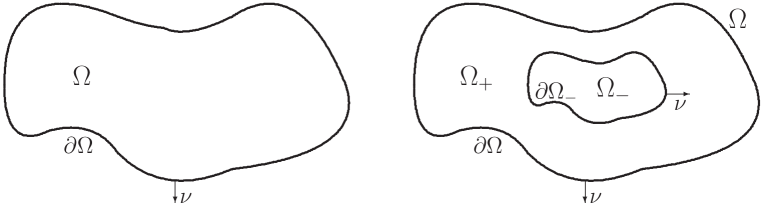
Figure 1: Geometric illustration of the problem: (left) a bounded open set $\Omega\subset{\mathbb{R}}^{n}$ with a smooth boundary $\partial\Omega$, on which Dirichlet, Neumann or Robin boundary condition is imposed; (right) non empty open connected sets $\Omega_{-}$, $\Omega_{+}$, $\Omega\subset{\mathbb{R}}^{n}$ satisfying (1.4), with the transmission boundary condition imposed on $\partial\Omega_{-}$, and Neumann or Dirichlet condition imposed on $\partial\Omega$. The unit normal vector $\nu$ pointing outwards is also shown.

In addition, we shall address, as in [18], a Dirichlet condition on $\partial\Omega$ instead of a Neumann condition. To distinguish between these two situations, we write ${\mathcal{A}}_{h}^{TN}$ and ${\mathcal{A}}_{h}^{TD}$. Sometimes, we use the notation ${\mathcal{A}}_{h,\mathcal{K}}^{TD}$ to keep in mind the reference to the transmission parameter $\mathcal{K}$, which could be $h$-dependent. In the Dirichlet case, the form domain $H^{1}(\Omega_{-})\times H^{1}(\Omega_{+})$ should be replaced by $H^{1}(\Omega_{-})\times\tilde{H}^{1}(\Omega_{+})$, where $\tilde{H}^{1}(\Omega_{+})=\{u\in H^{1}(\Omega_{+})\,,\,u=0\mbox{ on }\partial\Omega\}$. The domain of the operator is then

$$D({\mathcal{A}}_{h}^{TD})=\{u=(u_{-},u_{+})\in H^{2}(\Omega_{-})\times H^{2}(\Omega_{+})\\ \hskip 40.00006pth^{2}\partial_{\nu}u_{-}=h^{2}\partial_{\nu}u_{+}=\mathcal{K}(u_{+}-u_{-})\mbox{ on }\partial\Omega_{-}\,,\,u_{+}=0\mbox{ on }\partial\Omega\}\,,$$ (1.7)

where $\nu$ is pointing outwards of $\Omega_{-}$ at the points of $\partial\Omega_{-}\,$.

The spectral analysis of the various realizations of ${\mathcal{A}}_{h}$ has several applications in mathematical physics, among them are the Orr-Sommerfeld equations in fluid dynamics [28], the Ginzburg-Landau equation in the presence of electric current (when magnetic field effects are neglected) [3, 5, 6, 7], the null controllability of Kolmogorov type equations [10], and the diffusion nuclear magnetic resonance [30, 31, 14]. In particular, the transmission problem naturally arises in diffusion or heat exchange between two sets separated by a partially permeable/isolating interface (see [15, 18] and references therein). In this setting, the first relation in (1.6) or (1.7) ensures the continuity of flux between two sets, whereas the second relation accounts for the drop of the transverse magnetization $u$ across the interface, with the transmission coefficient $\mathcal{K}$. As in [3, 26, 8] for the Dirichlet or Neumann case, we seek an approximation for $\inf{\rm Re\,}\sigma({\mathcal{A}}_{h}^{R})$, $\inf{\rm Re\,}\sigma({\mathcal{A}}_{h}^{TN})$ or $\inf{\rm Re\,}\sigma({\mathcal{A}}_{h}^{TD})$ as $h\to 0$ ($h>0$). In [26, 8, 18], various constructions of quasimodes give some idea for the location of the leftmost eigenvalue (i.e. with smallest real part).

In the following, we formulate the assumptions, the notation and the main statements of the paper.

Assumption 1.1.

The potential $V$ satisfies

$$\nabla V(x)\neq 0\,,\,\forall x\in\overline{\Omega}\,.$$

Since, aside from minor differences, the treatment of all boundary conditions is similar, we use a general notation that can describe all problems. Thus, we define $\Omega^{\#}$ by $\Omega^{\#}=\Omega$ if $\#=D,N,R$ and by $\Omega^{\#}=\Omega_{-}\cup\Omega_{+}$ in the transmission case: $\#=TD$ or $\#=TN$. Let $\partial\Omega_{\perp}^{\#}$ denote the subset of $\partial\Omega^{\#}$ where $\nabla V$ is orthogonal to $\partial\Omega^{\#}$:

$$\partial\Omega_{\perp}^{\#}=\{x\in\partial\Omega^{\#}:\nabla V(x)=(\nabla V(x)\cdot\vec{\nu}(x))\,\vec{\nu}(x)\}\,,$$ (1.8)

where $\vec{\nu}(x)$ denotes the outward normal on $\partial\Omega^{\#}$ at $x$ .

Let $\#\in\{D,N,R,T\}$ and $\mathfrak{D}^{\#}$ be defined in the following manner

$$\begin{cases}\mathfrak{D}^{\#}=\{u\in H^{2}_{loc}(\overline{{\mathbb{R}}_{+}})\,|\,u(0)=0\}&\#=D\\ \mathfrak{D}^{\#}=\{u\in H^{2}_{loc}(\overline{{\mathbb{R}}_{+}})\,|\,u^{\prime}(0)=0\}&\#=N\\ \mathfrak{D}^{\#}=\{u\in H^{2}_{loc}(\overline{{\mathbb{R}}_{+}})\,|\,u^{\prime}(0)=\kappa\,u(0)\}&\#=R\\ \mathfrak{D}^{\#}=\{u\in H^{2}_{loc}(\overline{{\mathbb{R}}_{-}})\times H^{2}_{loc}(\overline{{\mathbb{R}}_{+}})\,|\,u^{\prime}_{+}(0)=&\\ \kern 100.00015ptu^{\prime}_{-}(0)=\kappa\,[u_{+}(0)-u_{-}(0)]\}&\#=T\,.\end{cases}$$ (1.9)

In the two last cases we occasionally write $\mathfrak{D}^{\#}(\kappa)$ in order to emphasize the dependence on the Robin or transmission parameter $\kappa$. In the above $u_{\pm}=u|_{{\mathbb{R}}_{\pm}}$ if we identify $L^{2}(\mathbb{R}_{-}\cup\mathbb{R}_{+})$ and $L^{2}({\mathbb{R}}_{-})\times L^{2}({\mathbb{R}}_{+})$. We further set ${\mathbb{R}}_{\#}={\mathbb{R}}_{+}$ when $\#\in\{D,N,R\}$ and ${\mathbb{R}}_{\#}={\mathbb{R}}_{+}\cup{\mathbb{R}}_{-}$ for $\#=T$. Then, we define the operator

$$\mathcal{L}^{\#}({\mathfrak{j}})=-\frac{d^{2}}{dx^{2}}+i\,{\mathfrak{j}}\,x\,,$$

whose domain is given by

$$D(\mathcal{L}^{\#}({\mathfrak{j}}))=H^{2}({\mathbb{R}}^{\#})\cap L^{2}({\mathbb{R}}^{\#};|x|^{2}dx)\cap\mathfrak{D}^{\#}\,,$$ (1.10)

(where $H^{2}(\mathbb{R}_{-}\cup\mathbb{R}_{+})=H^{2}(\mathbb{R}_{-})\times H^{2}(\mathbb{R}_{+})$) and set

$$\lambda^{\#}({\mathfrak{j}})=\inf{\rm Re\,}\sigma(\mathcal{L}^{\#}({\mathfrak{j}}))\,.$$ (1.11)

Again, when $\kappa$ is involved, we occasionally write $\mathcal{L}^{\#}({\mathfrak{j}},\kappa)$, $\lambda^{\#}({\mathfrak{j}},\kappa)$.

Next, let

$$\Lambda_{m}^{\#}=\inf_{x\in\partial\Omega_{\perp}^{\#}}\lambda^{\#}(|\nabla V(x)|)\,,$$ (1.12)

In the transmission case, for $\#=T\flat$ with $\flat\in\{D,N\}$ the above formula should be interpreted as

$$\Lambda_{m}^{T\flat}(\kappa)=\min\left(\inf_{x\in\partial\Omega_{\perp}^{\#}\cap\partial\Omega_{-}}\lambda^{T}(|\nabla V(x)|,\kappa)\,,\inf_{x\in\partial\Omega_{\perp}^{\#}\cap\partial\Omega}\lambda^{\flat}(|\nabla V(x)|)\right)\,.$$ (1.13)

In all cases we denote by ${\mathcal{S}}^{\#}$ the set

$${\mathcal{S}}^{\#}=\{x\in\partial\Omega_{\perp}^{\#}\,:\,\lambda^{\#}(|\nabla V(x)|,\kappa)=\Lambda_{m}^{\#}(\kappa)\,\}\,.$$ (1.14)

When $\#\in\{D,N\}$ it can be verified by a dilation argument that, when ${\mathfrak{j}}>0\,$,

$$\lambda^{\#}({\mathfrak{j}})=\lambda^{\#}(1)\,{\mathfrak{j}}^{2/3}\,,$$ (1.15)

and when $\#\in\{R,T\}$ with parameter $\kappa\geq 0$ that (see Sections 2 and 3),

$$\lambda^{\#}({\mathfrak{j}},\kappa)=\lambda^{\#}(1,\kappa\,{\mathfrak{j}}^{-\frac{1}{3}})\,{\mathfrak{j}}^{2/3}\,.$$ (1.16)

For the Robin case ($\#=R$) we establish in Appendix B that $\lambda^{R}({\mathfrak{j}},\kappa)$ is monotonously increasing with ${\mathfrak{j}}$. Hence, for $\#\in\{D,N,R\}$ we have for

$${\mathfrak{j}}_{m}=\min_{x\in\partial\Omega_{\perp}}|\nabla V(x)|\,,$$ (1.17)

the property

$$\Lambda_{m}^{\#}=\lambda^{\#}({\mathfrak{j}}_{m})\,,\mbox{ for }\#\in\{D,N\}\,,\,\Lambda_{m}^{R}(\kappa)=\lambda^{R}({\mathfrak{j}}_{m},\kappa)\,.$$

For the transmission case $\#=T\flat$ (with $\flat=D$ or $\flat=N$), as the monotonicity of ${\mathfrak{j}}\mapsto\lambda^{T}({\mathfrak{j}},\kappa)$ has not been established, it is more difficult to define ${\mathfrak{j}}_{m}$ and we shall refrain from using it.

We next make the following additional assumption:

Assumption 1.2.

At each point $x$ of ${\mathcal{S}}^{\#}$,

$$\alpha(x)=\text{\rm det}D^{2}V_{\partial}(x)\neq 0\,,$$ (1.18)

where $V_{\partial}$ denotes the restriction of $V$ to $\partial\Omega^{\#}$, and $D^{2}V_{\partial}$ denotes its Hessian matrix.

It can be easily verified that (1.18) implies that $\mathcal{S}^{\#}$ is finite. Equivalently we may write

$$\alpha(x)=\Pi_{i=1}^{n-1}\alpha_{i}(x)\neq 0\,,$$ (1.19a)

where

$$\{\alpha_{i}\}_{i=1}^{N-1}=\sigma(D^{2}V_{\partial})\,,$$ (1.19b)

where each eigenvalue is counted according to its multiplicity.

The following has been established by R. Henry in [26]

Theorem 1.3.

Under Assumptions 1.1 and 1.2, we have

$$\varliminf\limits_{h\to 0}\frac{1}{h^{2/3}}\inf\bigl{\{}{\rm Re\,}\,\sigma(\mathcal{A}_{h}^{D})\bigr{\}}\geq\Lambda_{m}^{D}\,,\qquad\Lambda_{m}^{D}=\frac{|a_{1}|}{2}{\mathfrak{j}}_{m}^{2/3}\,,$$ (1.20)

where $a_{1}<0$ is the rightmost zero of the Airy function Ai  . Moreover, for every $\varepsilon>0\,$, there exist $h_{\varepsilon}>0$ and $C_{\varepsilon}>0$ such that

$$\forall h\in(0,h_{\varepsilon}),~{}~{}~{}\sup_{\begin{subarray}{c}\gamma\leq\Lambda_{m}^{D}\\[1.50694pt] \nu\in\mathbb{R}\end{subarray}}\|(\mathcal{A}_{h}^{D}-(\gamma-\varepsilon)h^{2/3}-i\nu)^{-1}\|\leq\frac{C_{\varepsilon}}{h^{2/3}}\,.$$ (1.21)

In its first part, this result is essentially a reformulation of the result stated by the first author in [3]. Note that the second part provides, with the aid of the Gearhart-Prüss theorem, an effective bound (with respect to both $t$ and $h$) of the decay of the associated semi-group as $t\to+\infty\,$. The theorem holds in particular in the case $V(x)=x_{1}$ where $\Omega$ is a disk (and hence $S^{T}$ consists of two points) and in the case of an annulus (four points). Note that ${\mathfrak{j}}_{m}=1$ in this case.

A similar result can be proved for the Neumann case where (1.20) is replaced by

$$\varliminf\limits_{h\to 0}\frac{1}{h^{2/3}}\inf\bigl{\{}{\rm Re\,}\,\sigma(\mathcal{A}_{h}^{N})\bigr{\}}\geq\Lambda_{m}^{N}\,,\qquad\Lambda_{m}^{N}=\frac{|a^{\prime}_{1}|}{2}\,{\mathfrak{j}}_{m}^{2/3}\,,$$ (1.22)

where $a^{\prime}_{1}<0$ is the rightmost zero of $\text{\rm Ai\,}^{\prime}$, and (1.21) is replaced by

$$\forall h\in(0,h_{\varepsilon}),~{}~{}~{}\sup_{\begin{subarray}{c}\gamma\leq\Lambda_{m}^{N}\\[1.50694pt] \nu\in\mathbb{R}\end{subarray}}\|(\mathcal{A}_{h}^{N}-(\gamma-\varepsilon)h^{2/3}-i\nu)^{-1}\|\leq\frac{C_{\varepsilon}}{h^{2/3}}\,.$$ (1.23)

We establish here the corresponding results, for both the Robin boundary condition and the various Transmission problems.

Theorem 1.4.

Under Assumptions 1.1 and 1.2,

$$\varliminf\limits_{h\to 0}\frac{1}{h^{2/3}}\inf\bigl{\{}{\rm Re\,}\,\sigma(\mathcal{A}_{h,\mathcal{K}(h)}^{R})\bigr{\}}\geq\Lambda_{m}^{R}(\kappa),\qquad\Lambda_{m}^{R}(\kappa)=\lambda^{R}({\mathfrak{j}}_{m},\kappa)\,,$$ (1.24)

where $\mathcal{A}_{h,\mathcal{K}}^{R}$ is the Robin realization (with parameter $\mathcal{K}\geq 0$) of $\mathcal{A}_{h}$ , and $\mathcal{K}=\mathcal{K}(h)$ satisfies (1.3).
Moreover, for every $\varepsilon>0\,$, there exist $h_{\varepsilon}>0$ and $C_{\varepsilon}>0$ such that

$$\forall h\in(0,h_{\varepsilon}),~{}~{}~{}\sup_{\begin{subarray}{c}\gamma\leq\Lambda_{m}^{R}(\kappa),\\[1.50694pt] \nu\in\mathbb{R}\end{subarray}}\|(\mathcal{A}_{h,\mathcal{K}(h)}^{R}-(\gamma-\varepsilon)h^{2/3}-i\nu)^{-1}\|\leq\frac{C_{\varepsilon}}{h^{2/3}}\,.$$ (1.25)

Theorem 1.5.

Under Assumptions 1.1 and 1.2,

$$\varliminf\limits_{h\to 0}\frac{1}{h^{2/3}}\inf\bigl{\{}{\rm Re\,}\,\sigma(\mathcal{A}_{h,\mathcal{K}(h)}^{T\flat})\bigr{\}}\geq\Lambda_{m}^{T\flat}(\kappa)\,,$$ (1.26)

where $\mathcal{A}_{h,\mathcal{K}}^{T\flat}$ is the $T\flat$-realization (with parameter $\mathcal{K}\geq 0$) of $\mathcal{A}_{h}$ with $\flat$-condition on $\partial\Omega$ ( $\flat\in\{D,N\}$) and $T$-condition along $\partial\Omega_{-}$ and $\mathcal{K}=\mathcal{K}(h)$ satisfies (1.3).
Moreover, for every $\varepsilon>0\,$, there exist $h_{\varepsilon}>0$ and $C_{\varepsilon}>0$ such that

$$\forall h\in(0,h_{\varepsilon}),~{}~{}~{}\sup_{\begin{subarray}{c}\gamma\leq\Lambda_{m}^{T\flat}(\kappa),\\[1.50694pt] \nu\in\mathbb{R}\end{subarray}}\|(\mathcal{A}_{h,\mathcal{K}(h)}^{T\flat}-(\gamma-\varepsilon)h^{2/3}-i\nu)^{-1}\|\leq\frac{C_{\varepsilon}}{h^{2/3}}\,.$$ (1.27)

We now look at upper bounds for the left margin of the spectrum. Our main theorem is:

Theorem 1.6.

Under Assumptions 1.1 and 1.2, for $\#\in\{D,N,R,T\flat\}$ with $\flat\in\{D,N\}$, one has

$$\varlimsup\limits_{h\to 0}\frac{1}{h^{2/3}}\inf\bigl{\{}{\rm Re\,}\,\sigma(\mathcal{A}_{h,\mathcal{K}(h)}^{\#})\bigr{\}}=\Lambda_{m}^{\#}(\kappa)\,,$$ (1.28)

where $\mathcal{K}(h)$ satisfies (1.3).

Remark 1.7.

An immediate conclusion which follows from the previous statements is that under Assumptions 1.1 and 1.2, for $\#\in\{D,N,R,T\flat\}$ with $\flat\in\{D,N\}$, we have

$$\lim_{h\to 0}\frac{1}{h^{2/3}}\inf\bigl{\{}{\rm Re\,}\,\sigma(\mathcal{A}_{h,\mathcal{K}(h)}^{\#})\bigr{\}}=\Lambda_{m}^{\#}(\kappa)\,,$$ (1.29)

where $\mathcal{K}(h)$ satisfies (1.3) .

In the case of the Dirichlet problem, this theorem was obtained in [8, Theorem 1.1] under the stronger assumption that, at each point $x$ of ${\mathcal{S}}^{D}$, the Hessian of $V_{\partial}:=V_{/\partial\Omega^{\#}}$ is positive definite if $\partial_{\nu}V(x)<0\,$ or negative definite if $\partial_{\nu}V(x)>0\,$, with $\partial_{\nu}V:=\nu\cdot\nabla V$. This additional assumption reflects some technical difficulties in the proof, that we overcome in Section 7 by using tensor products of semigroups, a point of view that is missing [8]. This generalization allows us to obtain the asymptotics of the left margin of $\sigma({\mathcal{A}}_{h}^{\#})$, for instance, when $V(x_{1},x_{2})=x_{1}$ and $\Omega$ is either an annulus or the exterior of a disk, where the above assumption is not satisfied. For this particular potential, an extension to the case when $\Omega$ is unbounded is of significant interest in the physics literature [17]. We may assume in this case that $\partial\Omega^{\#}$ is bounded and add for the potential $V$ the assumption (having in mind the case $V=x_{1}$) that there exist a compact set $K$ and positive constants $c$, $C$ such that, $\forall x\notin K\,$, $c\leq|\nabla V(x)|$ and $\sum_{1\leq|\alpha|\leq 2}|\partial_{x}^{\alpha}V(x)|\leq C$ . We leave this problem to future research.

The rest of this paper is organized as follows:
In the next section we briefly review properties of the Robin realization of the complex Airy operator in ${\mathbb{R}}_{+}$ that were established in [19], and extend them slightly further to accommodate our needs in the sequel. We do the same in Section 3 for the transmission problem. In Section 4 we consider the operator $-\Delta+iJ\cdot x$ (for some $J\in{\mathbb{R}}^{n}$) in ${\mathbb{R}}^{n}$ and in the half-space, where the boundary set on the hyperplane $x_{n}=0$. Most of the results in this section have been obtained in [26, 3], but some refined semigroup and resolvent estimates that are necessary in the last section are provided as well. In Section 5 we characterize the domain of operators with quadratic potential both in ${\mathbb{R}}^{n}$ (in fact, we address there a much more general class of operators) and in the presence of a boundary or an interface (the half-space). In Section 6 we prove Theorems 1.4 and 1.5. In the last section 7 we prove Theorem 1.6. Finally, in Appendix A we prove a simple inequality to assist the reader, and in Appendix B, we provide more information on the monotonicity of the real part of the eigenvalue of the one-dimensional complex Airy operator with respect to a parameter, which is less crucial for the sake of proving lower and upper bounds for $\inf{\rm Re\,}\sigma({\mathcal{A}}_{h})$, than what is covered in Sections 2 and 3 but allows for a simpler formulation of some of the results.

2 The complex Airy operator on the half-line: Robin case

For ${\mathfrak{j}}\neq 0$ and $\kappa\geq 0$, we consider

$$\mathcal{L}^{R}(\mathfrak{j},\kappa)=-\frac{d^{2}}{dx^{2}}+i\,\mathfrak{j}\,x$$ (2.1)

defined on (cf. [19])

$$D(\mathcal{L}^{R}(\mathfrak{j},\kappa))=\{u\in H^{2}({\mathbb{R}}_{+},{\mathbb{C}})\cap L^{2}({\mathbb{R}}_{+},{\mathbb{C}}\,;\,x^{2}dx)\,|\,u^{\prime}(0)=\kappa\,u(0)\,\}\,.$$ (2.2)

The operator is associated with the sesquilinear form defined on $H^{1}({\mathbb{R}}_{+},{\mathbb{C}})\times H^{1}({\mathbb{R}}_{+},{\mathbb{C}})$ by

$$a^{R}(u,v)=\int_{0}^{+\infty}u^{\prime}(x)\,\bar{v}^{\prime}(x)\,dx+i\,{\mathfrak{j}}\int_{0}^{+\infty}x\,u(x)\,\bar{v}(x)\,dx+\kappa\,u(0)\,\bar{v}(0)\,.$$

We begin by recalling some of the results of [19] with the Robin boundary condition which naturally extends from both Dirichlet and Neumann cases. One should be more careful with the dilation argument.
Dilation argument.
For ${\mathfrak{j}}>0$, if $U_{\mathfrak{j}}\in\mathcal{L}(L^{2}({\mathbb{R}}_{+},{\mathbb{C}}))$ denotes the following unitary dilation operator

$$(U_{\mathfrak{j}}u)(x)=\mathfrak{j}^{1/3}u(\mathfrak{j}^{1/3}\,x)\,,$$

we observe that

$$\mathcal{L}^{R}(1,\mathfrak{j}^{-1/3}\kappa)=\mathfrak{j}^{2/3}U_{\mathfrak{j}}^{-1}\mathcal{L}^{R}(\mathfrak{j},\kappa)U_{\mathfrak{j}}\,,$$ (2.3)

It is then enough by dilation to consider the case ${\mathfrak{j}}=\pm 1$, but with a new Robin parameter and by using the complex conjugation ${\mathfrak{j}}=1$.

In the Robin case, the distribution kernel (or the Green’s function) of the resolvent is given by

$$\mathcal{G}^{R}(x,y\,;\lambda)=\mathcal{G}_{0}(x,y\,;\lambda)+\mathcal{G}_{1}^{R}(x,y\,;\kappa,\lambda)\,\quad\textrm{for}~{}(x,y)\in\mathbb{R}_{+}^{2}\,,$$

where

$$\begin{split}\mathcal{G}^{R}_{1}(x,y\,;\kappa,\lambda)&=-2\pi\frac{ie^{-i2\pi/3}\text{\rm Ai\,}^{\prime}(e^{-i2\pi/3}\lambda)+\kappa\,\text{\rm Ai\,}(e^{-i2\pi/3}\lambda)}{ie^{i2\pi/3}\text{\rm Ai\,}^{\prime}(e^{i2\pi/3}\lambda)+\kappa\,\text{\rm Ai\,}(e^{i2\pi/3}\lambda)}\\ &\times\text{\rm Ai\,}\bigl{(}e^{i2\pi/3}(-ix+\lambda)\bigr{)}~{}\text{\rm Ai\,}\bigl{(}e^{i2\pi/3}(-iy+\lambda)\bigr{)}\,,\\ \end{split}$$ (2.4)

and $\mathcal{G}_{0}(x,y\,;\lambda)$ is the resolvent of $D_{x}^{2}+ix$ on ${\mathbb{R}}$, which is an entire function of $\lambda$.

Setting $\kappa=0\,$, one retrieves the Neumann case, while the limit $\kappa\to+\infty$ yields the Dirichlet case. As in the Dirichlet case [3, 26], the resolvent is compact and in the Schatten class $\mathcal{C}^{p}$ for any $p>\frac{3}{2}$. Its (complex-valued) poles are determined by solving the equation

$$f^{R}(\kappa,\lambda):=ie^{-i2\pi/3}\text{\rm Ai\,}^{\prime}(e^{-i2\pi/3}\lambda)-\kappa\text{\rm Ai\,}(e^{-i2\pi/3}\lambda)=0\,.$$ (2.5)

Denote by $\lambda_{j}^{R}(\kappa)$ ($j\in\mathbb{N}^{*}$) the sequence of eigenvalues that we order by their non decreasing real part. Except for the case of small (respectively. large) $\kappa$, in which the eigenvalues can be shown to be close to the eigenvalues of the Neumann (respectively Dirichlet) problem, it does not seem easy to obtain the precise value of $\lambda_{j}^{R}$ for any $j\in\mathbb{N}$. Nevertheless, one can prove that the zeros of $f^{R}(\kappa,\cdot)$ are simple. If indeed $\lambda$ is a common zero of $f^{R}$ and $(f^{R})^{\prime}$, then either $\lambda+\kappa^{2}=0$, or $e^{-i2\pi/3}\lambda$ is a common zero of Ai  and $\text{\rm Ai\,}^{\prime}$. The second option is excluded by uniqueness of the trivial solution for the initial value problem $-u^{\prime\prime}+zu=0$, $u(z_{0})=u^{\prime}(z_{0})=0$, whereas the first option is excluded for $\kappa\geq 0$ because the spectrum is contained in the positive half-plane.

Since the numerical range of the Robin realization of $D_{x}^{2}+ix$ is contained in the first quadrant of the complex plane we have

Proposition 2.1.

$$\|\mathcal{G}^{R}(\kappa,\lambda)\|\leq\frac{1}{|{\rm Re\,}\lambda|}\,,\,\mbox{ if }{\rm Re\,}\lambda<0\,,$$ (2.6a)

and

$$\|\mathcal{G}^{R}(\kappa,\lambda)\|\leq\frac{1}{|{\rm Im\,}\lambda|}\,,\,\mbox{ if }{\rm Im\,}\lambda<0\,.$$ (2.6b)

The above, together with the Phragmén-Lindelöf principle (see [2]) and the fact that the resolvent is in $\mathcal{C}^{p}$, for any $p>\frac{3}{2}$, implies (after a dilation to treat general ${\mathfrak{j}}$) the proposition:

Proposition 2.2.

For any $\kappa\geq 0$ and ${\mathfrak{j}}\neq 0$, the space generated by the eigenfunctions of $\mathcal{L}^{R}(\mathfrak{j},\kappa)$ is dense in $L^{2}({\mathbb{R}}_{+},{\mathbb{C}})$.

We conclude this section with some semigroup estimates.

Proposition 2.3.

Let $\lambda^{R}(\mathfrak{j},\kappa)$ denote the real value of the leftmost eigenvalue of $\mathcal{L}^{R}(\mathfrak{j},\kappa)$. Then for any positive $\mathfrak{j}_{0}\,$, $\mathfrak{j}_{1}$, $\kappa_{0}$ and $\epsilon$ there exists $C(\mathfrak{j}_{0},\mathfrak{j}_{1},\kappa_{0},\epsilon)>0$ such that, for $0<\mathfrak{j}_{0}\leq\mathfrak{j}\leq\mathfrak{j}_{1}$ and $\kappa\in[0,\kappa_{0}]$,

$$\|e^{-t\mathcal{L}^{R}(\mathfrak{j},\kappa)}\|\leq{C(\mathfrak{j}_{0},\mathfrak{j}_{1},\kappa_{0},\epsilon)}\,e^{-t(\lambda^{R}(\mathfrak{j},\kappa)-\epsilon)}\,.$$ (2.7)

Proof.

As already observed, it suffices to consider the dependence of $\|e^{-t\mathcal{L}^{R}(1,\kappa^{*})}\|$ on

$$\kappa^{*}=\mathfrak{j}^{-1/3}\kappa\,.$$ (2.8)

Recall that $\lambda_{1}^{R}(\kappa^{*})=\lambda_{1}^{R}(1,\kappa^{*})$ denotes the leftmost eigenvalue of $\mathcal{L}^{R}(1,\kappa^{*})$. Since $\lambda^{R}_{1}(\kappa^{*})$ is a simple zero of solution of $f^{R}(\kappa^{*},\lambda)$ it must be a $C^{1}$ function of $\kappa^{*}$ on $|0,+\infty)$ and since $\lambda^{R}(1,\kappa^{*})={\rm Re\,}\lambda_{1}^{R}(\kappa^{*})$ we readily obtain, for any bounded interval $[0,\kappa_{0}^{*}]$, that

$$\sup_{\kappa^{*}\in[0,\kappa_{0}^{*}]}\lambda^{R}(1,\kappa^{*})<+\infty\,.$$ (2.9)

Let then $\epsilon>0$ and

$$D_{\rho}=\{z\in{\mathbb{C}}\,|\,|z|\geq\rho,\;{\rm Re\,}z\leq\lambda^{R}(1,\kappa^{*})-\epsilon\,\}\,.$$

By applying the same technique as in [21, 19] we can prove that there exist $\rho_{0}>0$ and $C>0$ such that for all $\rho>\rho_{0}\,$,

$$\sup_{\kappa^{*}\in[0,\kappa_{0}^{*}]}\sup_{\lambda\in D_{\rho}(\kappa^{*})}\|(\mathcal{L}^{R}(1,\kappa^{*})-\lambda)^{-1}\|\leq C\,.$$ (2.10)

Next, let $|\lambda|<\rho$, and ${\rm Re\,}\lambda\leq\lambda^{R}(1,\kappa^{*})-\epsilon$. Here we can bound the resolvent norm by its Hilbert-Schmidt norm and then use (2.4) to obtain

$$\|(\mathcal{L}^{R}(1,\kappa^{*})-\lambda)^{-1}\|\leq C\,\Big{|}\frac{ie^{-i2\pi/3}\text{\rm Ai\,}^{\prime}(e^{-i2\pi/3}\lambda)+\kappa^{*}\text{\rm Ai\,}(e^{-2i\pi/3}\lambda)}{ie^{i2\pi/3}\text{\rm Ai\,}^{\prime}(e^{i2\pi/3}\lambda)+\kappa^{*}\text{\rm Ai\,}(e^{i2\pi/3}\lambda)}\Big{|}\,,$$

where $C$ is independent of $\kappa^{*}$ in $[0,\kappa_{0}^{*}]$. Hence, we may infer from the above and (2.9) that

$$\sup_{\kappa^{*}\in[0,\kappa_{0}^{*}]}\sup_{\begin{subarray}{r}\quad\qquad|\lambda|<\rho\\ \quad\qquad{\rm Re\,}\lambda\leq\lambda^{R}(1,\kappa^{*})-\epsilon\end{subarray}}\|(\mathcal{L}^{R}(1,\kappa^{*})-\lambda)^{-1}\|\leq C_{\epsilon}\,.$$

Combining the above with (2.10) yields that for some $M_{\epsilon}>0$

$$\sup_{\kappa^{*}\in[0,\kappa_{0}^{*}]}\sup_{{\rm Re\,}\lambda\leq\lambda^{R}(1,\kappa^{*})-\epsilon}\|(\mathcal{L}^{R}(1,\kappa^{*})-\lambda)^{-1}\|\leq M_{\epsilon}\,.$$

Since $M_{\epsilon}$ is independent of $\kappa^{*}\in[0,\kappa_{0}^{*}]$ we can deduce from the Gearhart-Prüss Theorem (cf. [20] or [29]) that for some $C_{\epsilon}>0$, independent of $\kappa^{*}\in[0,\kappa_{0}^{*}]$,

$$\|e^{-t\mathcal{L}^{R}(1,\kappa^{*})}\|\leq C_{\epsilon}e^{-t(\lambda^{R}(1,\kappa^{*})-\epsilon)}\,.$$

The proposition can now be proved by applying the inverse of (2.3).    

In Section 7 we will need a stronger estimate than (2.7).

Proposition 2.4.

Let $\lambda^{R}(\mathfrak{j},\kappa)$ denote the real value of the leftmost eigenvalue of $\mathcal{L}^{R}(\mathfrak{j},\kappa)$. Then for any positive $\kappa_{0}$, $\mathfrak{j}_{0}\,$ and $\mathfrak{j}_{1}$ there exists $C(\mathfrak{j}_{0},\mathfrak{j}_{1},\kappa_{0})>0$ such that, for $0<\mathfrak{j}_{0}\leq\mathfrak{j}\leq\mathfrak{j}_{1}$ and $\kappa\in[0,\kappa_{0}]$,

$$\|e^{-t\mathcal{L}^{R}(\mathfrak{j},\kappa)}\|\leq C(\mathfrak{j}_{0},\mathfrak{j}_{1},\kappa_{0})\,e^{-t\lambda^{R}(\mathfrak{j},\kappa)}\,.$$ (2.11)

Proof.

As in the previous proof, we can reduce after dilation the proof to the case $\mathfrak{j}=1$. We then need to control the uniformity of the various estimates with respect to $\kappa$ in $[0,\kappa_{0}/{\mathfrak{j}}_{0}^{\frac{1}{3}}]$ Denote by $(\lambda_{1}^{R}(\kappa),v_{1}^{R}(\cdot,\kappa))$ the eigenpair of $\mathcal{L}^{R}(1,\kappa)$ for which ${\rm Re\,}\lambda_{1}^{R}(\kappa)=\lambda^{R}(1,\kappa)$ and $\|v_{1}\|=1$. In [19] (see also Appendix B) we show that for any $\kappa\geq 0$, $\lambda_{1}^{R}(\kappa)$ is simple and unique. Let then $\Pi_{1}^{R}(\kappa)$ denote the projection on ${\rm span}(v_{1}^{R}(\cdot,\kappa))$, i.e,

$$u\mapsto\Pi_{1}^{R}(\kappa)u=\frac{\langle u,\bar{v}_{1}^{R}(\cdot,\kappa)\rangle}{|\langle v_{1}^{R}(\cdot,\kappa),\bar{v}_{1}^{R}(\cdot,\kappa)\rangle|}\,v_{1}^{R}(\cdot,\kappa)\rangle\,.$$ (2.12)

Clearly,

$$\|\Pi_{1}^{R}(\kappa)\|_{\mathcal{L}(L^{2}_{+})}=|\langle v_{1}^{R}(\cdot,\kappa),\bar{v}_{1}^{R}(\cdot,\kappa)\rangle|^{-1}\,.$$ (2.13)

We refer the reader to [19, Section 6 ] for the derivation of the above relation (where an explicit expression of $v_{1}^{R}$ in terms of Airy function is provided). It can be verified [18] that $\|\Pi_{1}^{R}\|$ is uniformly bounded when $\kappa$ belongs to any bounded interval in $\overline{{\mathbb{R}}_{+}}$.

Let $E_{1}=(I-\Pi_{1}^{R})L^{2}({\mathbb{R}}_{+})$, and $\mathcal{L}^{R,1}=\mathcal{L}^{R}(I-\Pi_{1}^{R})$. We may define $\mathcal{L}^{R,1}$ on $(I-\Pi_{1}^{R})D(\mathcal{L}^{R})$, which is clearly a dense set, in $L^{2}$ sense, in $E_{1}$. By Riesz-Schauder theory we have that

$$(\mathcal{L}^{R}-\lambda)^{-1}=\frac{\Pi_{1}^{R}}{\lambda-\nu_{1}}+T_{1}(\lambda,\kappa)\,,$$ (2.14)

where $T_{1}$ is holomorphic for all $\lambda$ satisfying ${\rm Re\,}\lambda<\lambda^{R,2}$, in which

$$\lambda^{R,2}={\rm Re\,}\lambda^{R}_{2}>\lambda^{R}\,.$$ (2.15)

By applying the same techniques as in the previous proposition we can prove that, for any $\kappa_{0}>0$ and $\epsilon>0$ there exists $C_{\epsilon}>0$ such that

$$\sup_{\kappa\in[0,\kappa_{0}]}\sup_{{\rm Re\,}\lambda\leq\lambda^{R,2}-\epsilon}\|T_{1}(\lambda)\|\leq C_{\epsilon}\,.$$ (2.16)

Restricting $T_{1}(\lambda)$ to $E_{1}$ (onto $D(\mathcal{L}^{R,1})$) we may write $T_{1}|_{E_{1}}=(\mathcal{L}^{R,1}-\lambda)^{-1}$. By (2.9) and the Gearhardt-Prüss Theorem we then obtain that for every $\epsilon>0$ there exists $C_{\epsilon}>0$ such that

$$\sup_{\kappa^{*}\in[0,\kappa_{0}^{*}]}\|e^{-t\mathcal{L}^{R,1}}\|\leq C_{\epsilon}e^{-(\lambda^{R,2}-\epsilon)t}\,.$$ (2.17)

We complete the proof of (2.11) by observing that

$$e^{-t\mathcal{L}^{R}}=e^{-t\mathcal{L}^{R}}\Pi_{1}^{R}+e^{-t\mathcal{L}^{R,1}}$$

and setting $\epsilon<\lambda^{R,2}-\lambda^{R}$.    

Remark 2.5.

The estimate (2.11) remains valid at $\kappa=0$, i.e., for Neumann boundary condition. For Dirichlet boundary conditions it is an immediate result of [8, Lemma 4.2].

We conclude this section by making the following simple observation

Lemma 2.6.

Under the previous assumptions, there exists $C({\mathfrak{j}}_{0},{\mathfrak{j}}_{1},\kappa_{0})$ such that if ${\mathfrak{j}}\in[{\mathfrak{j}}_{0},{\mathfrak{j}}_{1}]$ and $\kappa\in[0,\kappa_{0}]$ then

$$\Big{|}\frac{\partial\lambda^{R}_{1}}{\partial{\mathfrak{j}}}({\mathfrak{j}},\kappa)\Big{|}\leq C({\mathfrak{j}}_{0},{\mathfrak{j}}_{1},\kappa_{0})\,.$$ (2.18)

Proof.

The proof is immediate from the Feynman-Hellman formula

$$\Big{|}\frac{\partial\lambda^{R}_{1}}{\partial{\mathfrak{j}}}({\mathfrak{j}},\kappa)\Big{|}=i\frac{\langle x\,\bar{u}_{1}^{R},v_{1}^{R}\rangle}{\langle\bar{u}_{1}^{R},v_{1}^{R}\rangle}\,,$$

and from the fact that $\lambda^{R}_{1}$ is simple and hence $\langle\bar{u}_{1}^{R},v_{1}^{R}\rangle\neq 0\,$.    

3 The complex Airy operator with a semi-permeable barrier: definition and properties

For $\kappa\geq 0\,$, ${\mathfrak{j}}\neq 0$ and $\nu\geq 0\,$, we consider the sesquilinear form $a_{\nu}$ defined for $u=(u_{-},u_{+})$ and $v=(v_{-},v_{+})$ by

$$a_{\nu}^{T}(u,v) = \int_{-\infty}^{0}\Big{(}u_{-}^{\prime}(x)\,\bar{v}_{-}^{\prime}(x)+i\,{\mathfrak{j}}\,xu_{-}(x)\,\bar{v}_{-}(x)+\nu\,u_{-}(x)\,\bar{v}_{-}(x)\Big{)}\,dx$$ (3.1)

$$+\int_{0}^{+\infty}\Big{(}u_{+}^{\prime}(x)\,\bar{v}_{+}^{\prime}(x)+i\,{\mathfrak{j}}\,xu_{+}(x)\,\bar{v}_{+}(x)+\nu\,u_{+}(x)\,\bar{v}_{+}(x)\Big{)}\,dx$$

$$+\kappa\,\big{(}u_{+}(0)-u_{-}(0)\big{)}\big{(}\overline{v_{+}(0)-v_{-}(0)}\big{)}\,,$$

where the form domain $\mathcal{V}^{T}$ is

$$\mathcal{V}^{T}:=\Big{\{}u=(u_{-},u_{+})\in H_{-}^{1}\times H_{+}^{1}:|x|^{\frac{1}{2}}\,u\in L_{-}^{2}\times L_{+}^{2}\Big{\}}\,,$$

with $L_{\pm}^{2}=L^{2}(\mathbb{R}_{\pm})$, $H_{-}^{s}=H^{s}(\mathbb{R}_{\pm})$.

The space $\mathcal{V}$ is endowed with the Hilbertian norm

$$\|u\|_{\mathcal{V}}:=\sqrt{{\|u_{-}\|_{H_{-}^{1}}^{2}+\|u_{+}\|_{H_{+}^{1}}^{2}}+\||x|^{1/2}u\|_{L^{2}}^{2}}\,.$$

To give a precise mathematical definition of the associated closed operator, we cannot, due to the lack of coercivity, use the standard version of the Lax-Milgram theorem. In [19] a generalization of the Lax-Milgram theorem, introduced in [4], is used to obtain that

Proposition 3.1.

The operator $\mathcal{L}^{T}({\mathfrak{j}},\kappa)$ acting as

$$u\mapsto\mathcal{L}^{T}({\mathfrak{j}},\kappa)u=\left(-\frac{d^{2}}{dx^{2}}u_{-}+i\,{\mathfrak{j}}\,x\,u_{-}\,,\,-\frac{d^{2}}{dx^{2}}u_{+}+i\,{\mathfrak{j}}\,x\,u_{+}\right)$$

on the domain

$$\mathcal{D}(\mathcal{L}^{T}({\mathfrak{j}},\kappa))=\big{\{}u\in H_{-}^{2}\times H_{+}^{2}:x\,u\,\in L_{-}^{2}\times L_{+}^{2}\text{and }u\in\mathfrak{D}^{T}\big{\}}\,,$$ (3.2)

where $\mathfrak{D}^{T}(\kappa)$ is given by (1.9), is a closed operator with compact resolvent.
There exists some $\nu\in[0,+\infty)$ such that the operator $\mathcal{L}^{T}({\mathfrak{j}},\kappa)+\nu$ is maximal accretive.

Maximal accretiveness of $\mathcal{L}^{T}({\mathfrak{j}},\kappa)+\lambda$ for all $\lambda\in{\mathbb{R}}_{+}$ can be proved in the following manner. Denote by $(\mathcal{L}^{T}({\mathfrak{j}},\kappa))^{*}$ the adjoint of $\mathcal{L}^{T}({\mathfrak{j}},\kappa)$. By the above construction it is simply $\mathcal{L}^{T}(-{\mathfrak{j}},\kappa)$. Since $\mathcal{L}^{T}(\pm{\mathfrak{j}},\kappa)+\lambda$ is accretive whenever ${\rm Re\,}\lambda>0$, it follows by [13, Theorem II.3.17] that $\mathcal{L}^{T}({\mathfrak{j}},\kappa)+\lambda$ is maximal accretive, and hence generates a contraction semigroup.

As in the previous section we have

Proposition 3.2.

For any $\lambda\in\rho(\mathcal{L}^{T}({\mathfrak{j}},\kappa))$, $(\mathcal{L}^{T}({\mathfrak{j}},\kappa)-\lambda)^{-1}$ belongs to the Schatten class $\mathcal{C}^{p}$ for any $p>\frac{3}{2}$.

In contrast with the previous section, however, the numerical range of $\mathcal{L}^{T}({\mathfrak{j}},\kappa)$ is not embedded in the first quadrant of the complex plane, but instead covers its right half. Hence, we only have

$$\|\mathcal{L}^{T}({\mathfrak{j}},\kappa)-\lambda)^{-1}\|\leq\frac{1}{|{\rm Re\,}\lambda|}\,,\,\mbox{ if }{\rm Re\,}\lambda<0\,,$$ (3.3)

Since the above bound is not enough to establish completeness of the system of the eigenfunctions of $\mathcal{L}^{T}({\mathfrak{j}},\kappa)$ in $L_{-}^{2}\times L_{+}^{2}$ an additional estimate is necessary. It has been established in [19] that there exists $M>0$ such that for all $\lambda\in{\mathbb{R}}_{+}$ we have

$$\|(\mathcal{L}^{T}({\mathfrak{j}},\kappa)-\lambda)^{-1}\|\leq M(1+|\lambda|)^{-\frac{1}{4}}(\log\lambda)^{\frac{1}{2}}\,.$$

The above, together with (3.3), the Phragmén-Lindelöf principle, and the fact that the resolvent is in $\mathcal{C}^{p}$, for any $p>\frac{3}{2}$, implies, modulo the proof that all the eigenvalues are simple,

Proposition 3.3.

For any $\kappa\geq 0$, the space generated by the eigenfunctions of $\mathcal{L}^{T}({\mathfrak{j}},\kappa)$ is dense in $L^{2}_{-}\times L^{2}_{+}$.

We have hence to prove the simplicity. We can reduce the proof to ${\mathfrak{j}}=-1$. We recall from [19] that the eigenvalues of $\mathcal{L}^{T}(-1,\kappa)$ are determined by

$$f_{\kappa}\overset{def}{=}f(\lambda)+\frac{\kappa}{2\pi}=0\,,$$

where

$$f(\lambda)=\text{\rm Ai\,}^{\prime}(e^{i2\pi/3}\lambda)\,\text{\rm Ai\,}^{\prime}(e^{-i2\pi/3}\lambda)\,,$$

is entire.

Lemma 3.4.

All eigenvalues of $\mathcal{L}^{T}(-1,\kappa)$ are simple.

Proof.

Recall that if $\mu\in\sigma(\mathcal{L}^{T}(-1,\kappa))$ then

$$f(\mu)=\text{\rm Ai\,}^{\prime}(e^{i2\pi/3}\mu)\,\text{\rm Ai\,}^{\prime}(e^{-i2\pi/3}\mu)=-\kappa/2\pi\,.$$

Suppose further that $f^{\prime}(\mu)=0$. It has been established in [19] that

$$\text{\rm Ai\,}(e^{i2\pi/3}\mu)=\frac{e^{i\frac{\pi}{6}}}{2\kappa}\text{\rm Ai\,}^{\prime}(e^{i2\pi/3}\mu)\quad;\quad\text{\rm Ai\,}(e^{-i2\pi/3}\mu)=\frac{e^{-i\frac{\pi}{6}}}{2\kappa}\text{\rm Ai\,}^{\prime}(e^{-i2\pi/3}\mu)\,.$$ (3.4)

Let $u=(u_{+},u_{-})$ denote the eigenfunction associated with $\mu$. It can be easily verified that

$$\begin{cases}u_{-}(x)=C_{-}\text{\rm Ai\,}(-e^{i\pi/6}(x-i\mu))&x<0\\ u_{+}(x)=C_{+}\text{\rm Ai\,}(e^{-i\pi/6}(x-i\mu))&x>0\,.\end{cases}$$ (3.5)

We can now rewrite (3.4) in the following manner

$$u_{-}(0)=-\frac{1}{2\kappa}u_{-}^{\prime}(0)\quad;\quad u_{+}(0)=\frac{1}{2\kappa}u_{+}^{\prime}(0)$$

It follows that both $\mu$ and $\bar{\mu}$ are eigenvalues of $\bar{\mathcal{L}}^{R}(1,2\kappa)$. This is, however, a contradiction, as $\sigma(\bar{\mathcal{L}}^{R}(1,2\kappa))$ lies in the fourth quadrant, and since $\mu\notin{\mathbb{R}}$.    

Before providing some semigroup estimates, as in the previous section, we need to establish another auxiliary result.

Lemma 3.5.

Let $\omega\in{\mathbb{R}}_{+}$. Let $Z(\kappa,\omega)\in\mathbb{Z}_{+}$ denote the number of zeros of $f_{\kappa}$ for ${\rm Re\,}\lambda\leq\omega$. Then, for every $\kappa_{0}>0$ there exists $M(\omega,\kappa_{0})$ such that

$$\sup_{\kappa\in[0,\kappa_{0}]}Z(\kappa,\omega)\leq M(\omega,\kappa_{0})\,.$$ (3.6)

Proof.

Let

$$D_{\omega}=\{z\in{\mathbb{C}}\,|\,0\leq{\rm Re\,}z\leq\omega\}\,.$$

The number of zeros of $f_{\kappa}$ in $D_{\omega}$ is precisely $Z$ since there are no eigenvalues of $A_{1}^{+,T}$ in the left side of the complex plane (when $\kappa\geq 0$).
From the analysis of the resolvent for ${\rm Im\,}\lambda$ large (see [19]) and the continuity of the zeros, we deduce that there exists $L(\kappa_{0},\omega)$ such that, for all $\kappa\in[0,\kappa_{0}]$, the number of zeros of $f_{\kappa}$ in

$$D^{L}_{\omega}=\{z\in{\mathbb{C}}\,|\,0\leq{\rm Re\,}z\leq\omega\;;\;|z|\leq L(\kappa_{0},\omega)\}\,,$$

is precisely $Z(\kappa,\omega)$.

To prove (3.6) we now argue by contradiction. Suppose that there exists $\{\kappa_{j}\}_{j=1}^{\infty}\subset[0,\kappa_{0}]$ such that $Z(\kappa_{j},\omega)\to\infty$. Without loss of generality we assume $\kappa_{j}\to\kappa_{\infty}$, otherwise we move to a subsequence. Let $\mathcal{C}$ denote a closed path in ${\mathbb{C}}\setminus D^{L}_{\omega}$ enclosing $D_{\omega}^{L}$ such that $f_{\kappa_{\infty}}\neq 0$ on $\mathcal{C}$. For sufficiently large $j$, $f_{\kappa_{j}}\neq 0$ on $\mathcal{C}$ and we may use Rouché’s theorem to obtain

$$\frac{1}{2\pi i}\oint_{\mathcal{C}}\frac{f^{\prime}}{f_{\kappa_{j}}}d\lambda\to+\infty\,,$$

leading to a contradiction as

$$\frac{1}{2\pi i}\oint_{\mathcal{C}}\frac{f^{\prime}}{f_{\kappa_{\infty}}}d\lambda<+\infty\,.$$

   

As in the previous section we prove a semigroup estimate.

Proposition 3.6.

Let $\lambda^{T}(\mathfrak{j},\kappa)$ denote the real value of the leftmost eigenvalue of $\mathcal{L}^{T}(\mathfrak{j},\kappa)$. Then for any positive $\mathfrak{j}_{0}<\mathfrak{j}_{1}$, $\kappa_{0}$ and $\epsilon$, there exists $C(\mathfrak{j}_{0},\mathfrak{j}_{1},\kappa_{0},\epsilon)>0$ such that, for any $\mathfrak{j}_{0}\leq\mathfrak{j}\leq\mathfrak{j}_{1}$ and $\kappa\in[0,\kappa_{0}]$

$$\|e^{-t\mathcal{L}^{T}(\mathfrak{j},\kappa)}\|\leq C(\mathfrak{j}_{0},\mathfrak{j}_{1},\kappa_{0},\epsilon)\,e^{-t(\lambda^{T}(\mathfrak{j},\kappa)-\epsilon)}\,.$$ (3.7)

We skip the proof as it is identical with the proof of Proposition 2.3. One can also improve the proposition in the following way:

Proposition 3.7.

Let $\mathfrak{j}_{0}<{\mathfrak{j}}_{1}$ and $\kappa_{0}$ be positive constants. Then, there exists $C(\mathfrak{j}_{0},\mathfrak{j}_{1},\kappa_{0})>0$ such that, for any $0<\mathfrak{j}_{0}\leq\mathfrak{j}\leq\mathfrak{j}_{1}$ and $\kappa\in[0,\kappa_{0}]$

$$\|e^{-t\mathcal{L}^{T}(\mathfrak{j},\kappa)}\|\leq C(\mathfrak{j}_{0},\mathfrak{j}_{1},\kappa_{0})\,e^{-t\lambda^{T}(\mathfrak{j},\kappa)}\,.$$ (3.8)

Proof.

The proof is similar to the proof of Proposition 2.4, and we provide therefore only its outlines. Let $\lambda\in\sigma(\mathcal{L}^{T})$. It has been proved in [19] that $\lambda\notin{\mathbb{R}}$ and that there are at least two complex conjugate eigenvalues with a real value equal to $\lambda^{T}$. With the proof of simplicity in mind, we get $K$ pairs of complex conjugate eigenvalues with same real part $\lambda^{T}(\mathfrak{j},\kappa)$ and $K({\mathfrak{j}},\kappa)$ is uniformly bounded by (3.6). Let $U_{K}={\rm span}\{u_{1},\ldots,u_{2K}\}$ denote the space spanned by all the eigenfunctions (and generalized eigenfunctions) of $\mathcal{L}^{T}$ corresponding to eigenvalues whose real value is equal to $\lambda^{T}$. Let

$$P_{k}^{T}=\sum_{\ell=1}^{2k}\Pi_{\ell}\,,$$

where $\Pi_{\ell}$ denotes the projection on $u_{\ell}$ defined in (2.12). Using the same technique as in the proof of Proposition 2.3, we then conclude for any $\epsilon>0$, the existence of $C_{\epsilon}({\mathfrak{j}}_{0},{\mathfrak{j}}_{1},\kappa_{0})>0$ such that

$$\|e^{-t\mathcal{L}^{T}}(I-P_{k}^{T})\|\leq C_{\epsilon}({\mathfrak{j}}_{0},{\mathfrak{j}}_{1},\kappa_{0})\,e^{-(\lambda^{T,2}-\epsilon)t}\,,$$ (3.9)

where

$$\lambda^{T,2}=\inf{\rm Re\,}\sigma\big{(}\mathcal{L}^{T}(I-P_{k}^{T})\big{)}>\lambda^{T}\,.$$ (3.10)

The proposition now follows from the fact that

$$\|e^{-t\mathcal{L}^{T}}P_{k}^{T}\|\leq\left(\sum_{\ell=1}^{2k}\|\Pi_{\ell}\|\right)\,e^{-\lambda^{T}t}\leq C({\mathfrak{j}}_{0},{\mathfrak{j}}_{1},\kappa_{0})e^{-\lambda^{T}t}\,.$$

   

We conclude this section by making the following simple observation

Lemma 3.8.

Let $0<{\mathfrak{j}}_{0}<{\mathfrak{j}}_{1}$ and $\kappa_{0}>0$. Then, there exists $C({\mathfrak{j}}_{0},{\mathfrak{j}}_{1},\kappa_{0})>0$ such that, for ${\mathfrak{j}}\in[{\mathfrak{j}}_{0},{\mathfrak{j}}_{1}]$ and $\kappa\in[0,\kappa_{0}]$,

$$\Big{|}\frac{\partial\lambda^{T}}{\partial{\mathfrak{j}}}({\mathfrak{j}},\kappa)\Big{|}\leq C({\mathfrak{j}}_{0},{\mathfrak{j}}_{1},\kappa_{0})\,.$$ (3.11)

The proof is identical with the proof of Lemma 2.6.

4 Limit problems: linear potential

In this section, we consider the simplified cases where $\Omega$ is either the entire space $\mathbb{R}^{n}$, or the half-space

$$\mathbb{R}_{+}^{n}=\{x=(x_{1},\dots,x_{n})\in\mathbb{R}^{n}:x_{n}>0\}.$$ (4.1)

Furthermore the potential $V$ will be assumed to be a linear function. We note that these relatively simple problems naturally arise in the semi-classical limit $h\to 0$ of $({\mathcal{A}}_{h}-\lambda)^{-1}$, where ${\mathcal{A}}_{h}$ is given by (1.1) or (1.6).

4.1 The entire space problem

In this subsection, we mainly refer to [21], and reformulate the $2$-dimensional statements therein in the $n$-dimensional setting. Let $\vec{J}=(J_{1},\dots,J_{n})\in\mathbb{R}^{n}$ and

$$\mathcal{A}_{0}=-\Delta+i\ell$$

acting on $L^{2}(\mathbb{R}^{n})\,$, where $\ell(x)=\vec{J}\cdot x\,$. Up to an orthogonal change of variable followed by the scale change $x\mapsto J^{2/3}x$, where we use the notation

$$J=|\vec{J}|\,,$$

we can assume that $\mathcal{A}_{0}$ has the form

$$\mathcal{A}_{0}=-\Delta+ix_{n}\,.$$

Let $x=(x^{\prime},x_{n})$. Applying a partial Fourier transform in $x^{\prime}$

$$\mathcal{F}(u)=(2\pi)^{-(n-1)/2}\int_{{\mathbb{R}}^{n-1}}e^{-i\omega^{\prime}\cdot x^{\prime}}\,dx^{\prime}\,,$$

we obtain the transformed operator on $L^{2}(\mathbb{R}_{\omega^{\prime}}^{n-1}\times\mathbb{R}_{x_{n}})$

$$\hat{{\mathcal{A}}}_{0}=-\partial_{x_{n}}^{2}+ix_{n}+|\omega^{\prime}|^{2}\,.$$

with domain

$$D(\hat{{\mathcal{A}}_{0}})=\big{\{}u\in L^{2}(\mathbb{R}^{n}),|\omega^{\prime}|^{2}u\in L^{2}(\mathbb{R}^{n}),\partial_{x_{n}}^{2}u\in L^{2}(\mathbb{R}^{n})\,,\,x_{n}u\in L^{2}(\mathbb{R}^{n})\big{\}}\,.$$

from which we easily obtain that

$$D(\mathcal{A}_{0})=\{u\in H^{2}(\mathbb{R}^{n})\,|\,x_{n}u\in L^{2}(\mathbb{R}^{n})\}\,.$$ (4.2)

Recalling that the complex Airy operator

$$\mathcal{L}=-\frac{d^{2}}{dx_{n}^{2}}+ix_{n}$$ (4.3)

on $L^{2}(\mathbb{R})$ has empty spectrum, we then get as in [21, Proposition $7.1$] the following lemma.

Lemma 4.1.

We have $\sigma(\mathcal{A}_{0})=\emptyset$, and for all $\omega\in\mathbb{R}$, there exists $C_{\omega}^{0}$ such that

$$\sup_{{\rm Re\,}z\leq\omega}\|(\mathcal{A}_{0}-z)^{-1}\|\leq C_{\omega}^{0}.$$ (4.4)

Proof.

Set

$${\mathcal{A}}_{0}=-\Delta_{x^{\prime}}+\mathcal{L}$$

(equivalently we may set $\overline{-\Delta_{x^{\prime}}\otimes I+I\otimes\mathcal{L}}$).
As

$$e^{-t{\mathcal{A}}_{0}}=e^{t\Delta_{x^{\prime}}}\otimes e^{-t\mathcal{L}}\,,$$

and since (see [11])

$$\|e^{-t\mathcal{L}}\|\leq e^{-\frac{t^{3}}{12}}\,,$$

we obtain that

$$\|e^{-t({\mathcal{A}}_{0}-z)}\|\leq e^{-\frac{t^{3}}{12}+t\,{\rm Re\,}z}\,.$$ (4.5)

Recalling that (see [11])

$$({\mathcal{A}}_{0}-z)^{-1}=\int_{0}^{+\infty}e^{-t({\mathcal{A}}_{0}-z)}dt\,,$$ (4.6)

we may conclude that for any $\omega>0$ we have

$$\sup_{{\rm Re\,}z\leq\omega}\|({\mathcal{A}}_{0}-z)^{-1}\|\leq\int_{0}^{+\infty}e^{-\frac{t^{3}}{12}+t\omega}\,dt\,.$$

As $\omega\to+\infty$, we have, using Laplace method,

$$\int_{0}^{+\infty}e^{-\frac{t^{3}}{12}+t\omega}\,dt\sim C\,\omega^{-\frac{1}{4}}\,e^{\frac{4}{3}\omega^{\frac{3}{2}}}\,,$$ (4.7)

which gives a more precise information on $C_{\omega}^{0}$. A universal upper bound is obtained in Appendix A.    

4.2 The half-space problem: Definitions

4.2.1 Notation

Let

$${\mathbb{R}}^{n}_{\pm}=\{(x_{1},\ldots,x_{n})\in{\mathbb{R}}^{n}\,|\,\pm x_{n}>0\}\,,$$

and $\vec{J}=(J^{\prime},J_{n})\in\mathbb{R}^{n}\setminus\{0\}$ where $J^{\prime}\in{\mathbb{R}}^{n-1}$. We study here the spectrum and the behavior of the resolvent of the operator

$${\mathcal{A}}^{\#}={\mathcal{A}}^{\#}(\vec{J}):=-\Delta+i\vec{J}\cdot x$$

acting on $L^{2}(\mathbb{R}_{+}^{n})$ or on $L^{2}({\mathbb{R}}^{n}_{-})\times L^{2}({\mathbb{R}}^{n}_{+})$.
Here the superscript $\#$ means that ${\mathcal{A}}^{\#}$ is defined on a subset of $\mathfrak{D}^{\#}_{n}$, where

$$\begin{cases}\mathfrak{D}^{\#}_{n}=\{u\in H^{2}_{loc}(\overline{{\mathbb{R}}_{+}^{n}})\,|\,u(x^{\prime},0)=0\}&\#=D\\ \mathfrak{D}^{\#}_{n}=\{u\in H^{2}_{loc}(\overline{{\mathbb{R}}_{+}^{n}})\,|\,u_{x_{n}}(x^{\prime},0)=0\}&\#=N\\ \mathfrak{D}^{\#}_{n}=\{u\in H^{2}_{loc}(\overline{{\mathbb{R}}_{+}^{n}})\,|\,u_{x_{n}}(x^{\prime},0)=\,\kappa\,u(x^{\prime},0)\}&\#=R\\ \mathfrak{D}^{\#}_{n}=\{u\in H^{2}_{loc}(\overline{{\mathbb{R}}_{-}^{n}})\times H^{2}_{loc}(\overline{{\mathbb{R}}_{+}^{n}})\,|\partial_{x_{n}}u_{+}(x^{\prime},0)=&\\ \kern 100.00015pt\partial_{x_{n}}u_{-}(x^{\prime},0)=\kappa[u_{+}-u_{-}]{(x^{\prime},0)}\}&\#=T\,.\end{cases}$$ (4.8)

Naturally, $\mathfrak{D}^{\#}_{n}$ depends on $\kappa\geq 0$, when $\#\in\{R,T\}$. We shall occasionally, therefore, write ${\mathcal{A}}^{\#}(\vec{J},\kappa)$ or ${\mathcal{A}}^{\#}(\kappa)$ to emphasize the dependence on the parameters. We now attempt to obtain the domain of definition of ${\mathcal{A}}^{\#}$ so that ${\mathcal{A}}^{\#}:D({\mathcal{A}}^{\#})\to L^{2}({\mathbb{R}}^{n}_{\#})$ is surjective (where ${\mathbb{R}}^{n}_{\#}={\mathbb{R}}^{n-1}\times{\mathbb{R}}_{\#}$). This has been accomplished for Dirichlet boundary conditions by R. Henry [26]. We now employ the same technique as in [26] to obtain $D({\mathcal{A}}^{\#})$ when $\#\in\{N,R,T\}$.

4.2.2 Definition by using the separation of variables

We set, as above, $x^{\prime}=(x_{1},\dots,x_{n-1})$ to be the $(n-1)$ first coordinates of a vector $x\in\mathbb{R}^{n}$ and $\vec{J}=(J^{\prime},J_{n})$, and then let

$$\mathcal{A}_{x^{\prime}}=\mathcal{A}_{x^{\prime}}(J^{\prime})=-\Delta_{x^{\prime}}+iJ^{\prime}\cdot x^{\prime}\,,$$ (4.9)

acting on $L^{2}({\mathbb{R}}^{n-1})$ and

$$\mathcal{L}_{x_{n}}^{\#}=\mathcal{L}_{x_{n}}^{\#}(J_{n})=-\frac{\partial^{2}}{\partial x_{n}^{2}}+iJ_{n}x_{n}\,,$$ (4.10)

acting on $L^{2}_{\#}$, which denotes either $L^{2}({\mathbb{R}}_{+},{\mathbb{C}})$ when $\#\in\{D,N,R\}$ or $L^{2}({\mathbb{R}}_{+},{\mathbb{C}})\times L^{2}({\mathbb{R}}_{-},{\mathbb{C}})$ for the transmission problem.
We recall that the domains of ${\mathcal{A}}_{x^{\prime}}$ and $\mathcal{L}_{x_{n}}^{\#}$ have been well identified in [3, 26, 19, 18] and that estimates for the resolvent have been established in each case (these depend on $J^{\prime}$, $J_{n}$ and on the value of $\#$ in $\{D,N,R,T\}$). In addition, it has been established, with the aid of the Hille-Yosida theorem, that both $\mathcal{A}_{x^{\prime}}$ and $\mathcal{L}_{x_{n}}^{\#}$ are generators of contraction semigroups $(e^{-t\mathcal{A}_{x^{\prime}}})_{t>0}$ and $(e^{-t\mathcal{L}_{x_{n}}^{\#}})_{t>0}$, respectively (recall that $\kappa\geq 0$ when $\#\in\{R,T\}$). It can be easily verified that the family $(e^{-t\mathcal{A}_{x^{\prime}}}\otimes e^{-t\mathcal{L}_{x_{n}}^{\#}})_{t>0}$ is a contraction semigroup in $L^{2}_{\#}$. Thus, we can define

Definition 4.2.

${\mathcal{A}}^{\#,sv}$ is the generator of the semigroup $(e^{-t\mathcal{A}_{x^{\prime}}}\otimes e^{-t\mathcal{L}_{x_{n}}^{\#}})_{t>0}\,$.

To derive the domain of the operator ${\mathcal{A}}^{\#,sv}$, we follow the approach of [26]. Recall, then, the following result (see [27, Theorem X.$49$]):

Theorem 4.3.

Let $\mathcal{A}$ be the generator of a contraction semigroup on a Hilbert space $\mathcal{H}$. Let $\mathcal{C}\subset\mathcal{D}(\mathcal{A})$ be a dense subset of $\mathcal{H}$, such that

$$e^{-t\mathcal{A}}\,\mathcal{C}\subset\mathcal{C}\,,$$ (4.11)

Then, $\ \mathcal{C}$ is a core for $\mathcal{A}\,$, that is

$$\mathcal{A}=\overline{\mathcal{A}_{/\mathcal{C}}}\,.$$

We now apply this theorem with $\mathcal{A}={\mathcal{A}}^{\#,sv}$ and

$$\mathcal{C}=\mathcal{D}(\mathcal{A}_{x^{\prime}})\odot\mathcal{D}(\mathcal{L}_{x_{n}}^{\#})$$ (4.12)

that is the set of all finite linear combinations of functions of the form $f\otimes g=f(x^{\prime})g(x_{n})$, where $f\in\mathcal{D}(\mathcal{A}_{x^{\prime}})$ and $g\in\mathcal{D}(\mathcal{L}_{x_{n}}^{\#})$.
Then it is clear that $\mathcal{C}$ satisfies the conditions of Theorem 4.3, hence

$${\mathcal{A}}^{\#,sv}=\overline{{\mathcal{A}^{\#,sv}}_{/\mathcal{C}}}\,.$$ (4.13)

Remark 4.4.

Instead of $\mathcal{D}(\mathcal{L}_{x_{n}}^{\#})$ in (4.12) we may use the span of the eigenfunctions of $\mathcal{L}_{x_{n}}^{\#}$. Note that it has been shown in [3, 26, 19] that this space is dense in $L^{2}_{\#}$. Furthermore, it is a subset of $\mathcal{S}_{\#}$ and (4.11) is still satisfied, and hence we may still apply to it Theorem 4.3. In this way, it is easier to estimate any expression involving functions in $\mathcal{C}$.

We may now conclude from (4.13) that the domain of $A^{\#,sv}$ is given by

$$\mathcal{D}({\mathcal{A}}^{\#,sv}) = \{u\in L^{2}_{\#}:\exists(u_{j})_{j\geq 1}\in\mathcal{C}^{\mathbb{N}}\,,~{}u_{j}\underset{\tiny{j\to+\infty}}{\overset{L^{2}_{\#}}{\longrightarrow}}u\,,$$ (4.14)

$$\quad\quad\quad\quad({\mathcal{A}}^{\#,sv}u_{j})_{j\geq 1}~{}\textrm{is a Cauchy sequence in }L^{2}_{\#}~{}\}\,.$$

Clearly, $(-\Delta+i\ell)u\in L^{2}_{\#}$ for any $u\in\mathcal{D}(\mathcal{A}^{\#,sv})$. Nevertheless, it is not obvious that $\Delta u\in L^{2}_{\#}$ (and hence also $\ell u\in L^{2}_{\#}$). In the following we obtain bounds on $\|u\|_{H^{2}(\mathbb{R}_{+}^{n})}$ and $\|\ell u\|_{L^{2}(\mathbb{R}_{+}^{n})}\,$ in terms of the graph norm $u\mapsto\sqrt{\|u\|_{2}^{2}+\|{\mathcal{A}}^{\#,sv}u\|^{2}_{2}}$, thereby allowing for a representation of $\mathcal{D}({\mathcal{A}}^{\#,sv})$, which is much more transparent than (4.13) or (4.14). We state the result for the Robin case only, as the statement for the transmission problem are similar.

Proposition 4.5.

If $|\vec{J}|=J\neq 0$, we have

$$\mathcal{D}({\mathcal{A}}^{R,sv})=H^{2}(\mathbb{R}_{+}^{n})\cap L^{2}(\mathbb{R}_{+}^{n};\ell(x)^{2}\,dx)\cap\mathfrak{D}^{R}_{n}\,.$$ (4.15)

Furthermore, for all $u\in\mathcal{D}({\mathcal{A}}^{R,sv})\,$, we have

$$\|\nabla u\|^{2}\leq{\rm Re\,}\langle{\mathcal{A}}^{R,sv}\,u\,,\,u\rangle\,,$$ (4.16)

and

$$\|\Delta u\|_{L^{2}(\mathbb{R}_{+}^{n})}^{2}+\|\ell u\|_{L^{2}(\mathbb{R}_{+}^{n})}^{2}\leq\|{\mathcal{A}}^{R,sv}u\|_{L^{2}(\mathbb{R}_{+}^{n})}^{2}+J\,\|\nabla u\|_{L^{2}(\mathbb{R}_{+}^{n})}\|u\|_{L^{2}(\mathbb{R}_{+}^{n})}\,.$$ (4.17)

Proof.

The proof below is adapted from Henry [26]. Let $u\in\mathcal{D}({\mathcal{A}}^{R,sv})$. By (4.14) there exists $(u_{j})_{j\geq 1}\in\mathcal{C}^{\mathbb{N}}$ such that $u_{j}\underset{\tiny{j\to+\infty}}{\overset{L^{2}}{\longrightarrow}}u$ and $(\mathcal{A}u_{j})_{j\geq 1}$ is a Cauchy sequence. Then, as

$${\rm Re\,}\langle\mathcal{A}v,v\rangle=\|\nabla v\|_{L^{2}(\mathbb{R}_{+}^{n})}^{2}+\kappa\int_{\mathbb{R}^{n-1}}|v(x^{\prime},0)|^{2}dx^{\prime}\geq\|\nabla v\|_{L^{2}(\mathbb{R}_{+}^{n})}^{2}\,,$$

(note that $\kappa\geq 0$) it follows that $(\nabla u_{j})_{j\geq 1}$ is a Cauchy sequence in $L^{2}(\mathbb{R}_{+}^{n})$, and hence

$$u_{j}\underset{\tiny{j\to+\infty}}{\overset{H^{1}}{\longrightarrow}}u\,,$$ (4.18)

and $u\in H^{1}(\mathbb{R}_{+}^{n})\,$.
At this stage, we have established that

$$\mathcal{D}({\mathcal{A}}^{R,sv})\subset H^{1}(\mathbb{R}_{+}^{n})\,.$$ (4.19)

Moreover the first trace of $u_{j}$ on $\{x_{n}=0\}$, which is defined by

$$(\gamma_{0}u_{j})(x^{\prime})=u_{j}(x^{\prime},0)\,,$$

converges to $\gamma_{0}u$ in $H^{\frac{1}{2}}(\mathbb{R}^{n-1})$. For the second trace, which is defined by

$$(\gamma_{1}u_{j})(x^{\prime})=\partial_{x_{n}}u_{j}(x^{\prime},0)\,,$$

we use standard elliptic estimates to obtain that $u\in H^{2}_{loc}({\mathbb{R}}^{n}_{+})$ and hence also that $\gamma_{1}u\in H^{-\frac{1}{2}}_{loc}(\mathbb{R}^{n-1})$. Consequently, the Robin boundary condition is satisfied by $u$ as well.
In order to prove (4.17), we write (all the norms denoting $L^{2}$ norms)

$$\|{\mathcal{A}}u_{j}\|^{2} = \langle(-\Delta+i\ell)u_{j},(-\Delta+i\ell)u_{j}\rangle$$ (4.20)

$$= \|\Delta u_{j}\|^{2}+\|\ell u_{j}\|^{2}+2{\rm Im\,}\langle-\Delta u_{j},\ell u_{j}\rangle\,.$$

Here we use the regularity of $u_{j}$ which follows from the fact that ${\mathcal{D}}(\mathcal{A}_{x^{\prime}})$ is given by (4.2) and ${\mathcal{D}}(\mathcal{L}^{R}_{x_{n}})$ by (2.2).
We now observe that

$$\langle-\Delta u_{j},\ell u_{j}\rangle=\int_{\mathbb{R}_{+}^{n}}\nabla u_{j}(x)\cdot\overline{\nabla(\ell u_{j})(x)}dx-\int_{\mathbb{R}^{n-1}}\partial_{x_{n}}u_{j}(x^{\prime},0)\ell(x^{\prime},0)\bar{u}_{j}(x^{\prime},0)\,dx^{\prime}\,.$$ (4.21)

Using the Robin condition, this reads

$$\langle-\Delta u_{j},\ell u_{j}\rangle=\int_{\mathbb{R}_{+}^{n}}\nabla u_{j}(x)\cdot\overline{\nabla(\ell u_{j})(x)}dx+\kappa\int_{\mathbb{R}^{n-1}}\ell(x^{\prime},0)|u_{j}(x^{\prime},0)|^{2}\,dx^{\prime}\,.$$ (4.22)

Hence we have

$${\rm Im\,}\langle-\Delta u_{j},\ell u_{j}\rangle = {\rm Im\,}\int_{\mathbb{R}_{+}^{n}}\nabla u_{j}(x)\cdot\overline{\nabla(\ell u_{j})(x)}\,dx$$

$$= {\rm Im\,}\int_{\mathbb{R}_{+}^{n}}\left(\vec{J}\cdot\nabla u_{j}(x)\right)\,\overline{u_{j}(x)}\,dx\,.$$

This implies

$$|{\rm Im\,}\langle-\Delta u_{j},\ell u_{j}\rangle|\leq J\,\|\nabla u_{j}\|\,\|u_{j}\|\,.$$

Thus, the estimate (4.17) holds for $u_{j}$ for all $1\leq j$. Consequently, $(u_{j})_{j\geq 1}$ is a Cauchy sequence in $L^{2}(\mathbb{R}_{+}^{n};|\ell(x)|^{2}dx)$ and $\Delta u_{j}$ is a Cauchy sequence in $L^{2}(\mathbb{R}^{n}_{+})$. Hence $u\in H^{1}(\mathbb{R}_{+}^{n})$, $\Delta u\in L^{2}(\mathbb{R}_{+}^{n})$ and $u$ satisfies the Robin condition. We can then use the regularity of the Robin Laplacian which follows from the regularity of the Neumann Laplacian (see [18]) in order to show that $u\in H^{2}(\mathbb{R}_{+}^{n})$. We have thus established that

$$\mathcal{D}({\mathcal{A}}^{R,sv})\subseteq\hat{{\mathcal{D}}}\overset{def}{=}H^{2}(\mathbb{R}_{+}^{n})\cap L^{2}(\mathbb{R}_{+}^{n};\ell(x)^{2}\,dx)\cap\mathfrak{D}^{R}_{n}\,.$$

The proof of the converse inclusion goes as follows. Let $u\in\hat{{\mathcal{D}}}$. Clearly $f=(-\Delta+i\ell+1)u\in L^{2}({\mathbb{R}}^{n}_{+})$. Since $-\Delta+i\ell+1:\mathcal{D}({\mathcal{A}}^{R,sv})\to L^{2}({\mathbb{R}}^{n}_{+})$ is surjective, it follows that there exists $v\in\mathcal{D}({\mathcal{A}}^{R,sv})$ such that $(-\Delta+i\ell+1)v=f$. Thus $w=u-v\in\hat{{\mathcal{D}}}$ and satisfies $(-\Delta+i\ell+1)w=0$. By the injectivity of $(-\Delta+i\ell+1)$ on $\hat{\mathcal{D}}$ we obtain that $u=v$ and hence $\hat{{\mathcal{D}}}\subseteq\mathcal{D}({\mathcal{A}}^{R,sv})$.    

Remark 4.6.

Similar arguments lead to the proof of the same statement for the transmission case.

Remark 4.7.

Using [4, Theorem 2.1], we can also define the operator via a generalized Lax-Milgram lemma (see also [18]). It can be shown that the two definitions coincide. This approach has the advantage that it is applicable in cases where the potential is not a sum of potentials with separate variables. Nevertheless, we may apply the Lax-Milgram approach only under the following assumption on $V$:

$$|\nabla V|\leq C\sqrt{1+V(x)^{2}}\,.$$ (4.23)

We note that in the next section we consider potentials that are neither separable nor satisfy (4.23). However, since in Section 7 we will consider again a separable potential, preference was given to the separation of variables technique over the other approach.

4.3 Determination of the spectrum

Once ${\mathcal{A}}^{\#}$ has been defined in Definition 4.2 (we occasionally write it as either ${\mathcal{A}}^{\#}(\vec{J})$ or ${\mathcal{A}}^{\#}(J,\theta,\vec{v})$ with $\theta\in(-\pi,+\pi]$ to emphasize the dependence on the parameters), we can focus our attention on its spectrum $\sigma({\mathcal{A}}^{\#}((J,\theta,\vec{v})))$ and on its resolvent.

Proposition 4.8.

Let $\vec{J}:=(J^{\prime},J_{n})=J\,(\sin\theta\,\vec{v},\cos\theta)\,$, where $\vec{v}\in\mathbb{S}^{n-2}$ and $J>0$. Then:

• If $\theta\neq 0,\pi\,$, we have $\sigma({\mathcal{A}}^{\#}(J,\theta,\vec{v}))=\emptyset\,$.

• Otherwise, we have

  $$\sigma({\mathcal{A}}^{\#}(J,0,\vec{v}))=\mathop{\bigcup}\limits_{r\geq 0}\{\sigma(\mathcal{L}^{\#}(J))+r\}\,,$$ (4.24)

  and

  $$\sigma({\mathcal{A}}^{\#}(J,\pi,\vec{v}))=\overline{\sigma({\mathcal{A}}^{\#}(J,0,\vec{v}))}\,.$$ (4.25)

Proof.

To prove (4.24) we apply the partial Fourier transform $\mathcal{F}$ defined by

$$(\mathcal{F}f)(\omega^{\prime},x_{n})=\int_{{\mathbb{R}}^{n-1}}e^{i\omega^{\prime}\cdot x^{\prime}}f(x^{\prime},x_{n})\,dx^{\prime}\,,$$ (4.26)

to ${\mathcal{A}}^{\#}$ to obtain (recall that $\theta=0$)

$$\widehat{\mathcal{A}}^{\#}:=\mathcal{F}\,{\mathcal{A}}^{\#}\,\mathcal{F}^{-1}=\mathcal{L}_{x_{n}}^{\#}+|\omega^{\prime}|^{2}\,.$$ (4.27)

As $\sigma({\mathcal{A}}^{\#})=\sigma\big{(}\widehat{\mathcal{A}}^{\#}\big{)}$ we readily obtain (4.24).    

Henry’s lemma [26, Lemma 2.8] can be extended to any realization $\#$ in the following way:

Proposition 4.9.

1. For every $\omega\in\mathbb{R}\,$, there exists $C_{\omega}>0$ such that

   $$\sup_{\tiny{{\rm Re\,}z\leq\omega}}\|({\mathcal{A}}^{\#}(J,\theta,\vec{v})-z)^{-1}\|\leq C_{\omega}\,\exp\Big{\{}\frac{C_{\omega}}{J|\sin\theta|}\Big{\}}\,.$$ (4.28)

2. Let $0<J_{0}<J_{1}$ and $\kappa_{0}>0$. There exists $K(J_{0},J_{1},\varepsilon,\kappa_{0})>0$ such that for all $\varepsilon>0\,$, $\vec{v}\in\mathbb{S}^{n-2}\,$, $J_{0}\leq J\leq J_{1}$, and $\kappa\in[0,\kappa_{0}]$

   $$\sup_{\tiny{\begin{array}[]{c}\theta\in[-\pi,\pi]\\ {\rm Re\,}z\leq\lambda^{\#}(J\cos\theta,\kappa)-\varepsilon\end{array}}}\|({\mathcal{A}}^{\#}(J,\theta,\vec{v})-z)^{-1}\|\leq K(J_{0},J_{1},\varepsilon,\kappa_{0})\,,$$ (4.29)

   where $\lambda^{\#}(J\cos\theta,\kappa)=\min{\rm Re\,}\sigma\big{(}\mathcal{L}^{\#}(J\cos\theta,\kappa)\big{)}$ (when $\#\in\{D,N\}$ the dependence on $\kappa$ should be omitted).

Proof.

Let $\mathcal{L}_{x_{n}}^{\#}$ be given by (4.10) and ${\mathcal{A}}_{x^{\prime}}$ be given by (4.9). When $\#\in\{R,T\}$ with $\#$-constant $\kappa$ we write $\mathcal{L}_{x_{n}}^{\#}(J\cos\theta,\kappa)$. As both ${\mathcal{A}}_{x^{\prime}}$ and $\mathcal{L}_{x_{n}}^{\#}(J\cos\theta)$ are maximal accretive, we may write

$$e^{-t{\mathcal{A}}^{\#}(J,\theta,\vec{v})}=e^{-t{\mathcal{A}}_{x^{\prime}}(J,\theta,\vec{v})}\otimes e^{-t\mathcal{L}_{x_{n}}^{\#}(J\cos\theta)}\,.$$ (4.30)

Note that, for $\pm\theta\in(0,\pi)\,$, we may apply the rescaling $x\mapsto(J\,|\sin\theta|)^{1/3}x\,$, to obtain

$$e^{-t{\mathcal{A}}_{x^{\prime}}(J,\theta,\vec{v})}=e^{-t(J|\sin\theta|)^{2/3}{\mathcal{A}}_{x^{\prime}}(1,\pm\pi/2,\vec{v})}\,,$$

Hence, by (4.5),

$$||e^{-t{\mathcal{A}}_{x^{\prime}}(J,\theta,\vec{v})}||\leq e^{-\frac{t^{3}}{12}(J|\sin\theta|)^{2}}\,.$$ (4.31)

From (4.30) and the fact that $e^{-t\mathcal{L}_{x_{n}}^{\#}(J\cos\theta)}$ is a contraction semi-group, we get

$$\|e^{-t\mathcal{A}^{\#}(J,\theta,\vec{v})}\|\leq e^{-\frac{1}{12}J^{2}\sin^{2}\theta\,t^{3}}\,.$$

Suppose first that $\omega\geq 1$. Using (4.6), this time for ${\mathcal{A}}^{\#}$, i.e.,

$$({\mathcal{A}}^{\#}-z)^{-1}=\int_{0}^{+\infty}e^{-t({\mathcal{A}}^{\#}-z)}dt\,,$$ (4.32)

we obtain from (A.1) that, for all ${\rm Re\,}z\leq\omega\,$,

$$\|({\mathcal{A}}^{\#}-z)^{-1}\|\leq\int_{0}^{+\infty}e^{-\frac{1}{12}J^{2}\sin\theta^{2}\,t^{3}+\omega t}\,dt\leq\frac{\sqrt{2\pi}}{[J|\sin\theta|]^{1/2}\omega^{1/4}}\exp\biggl{(}\frac{2\omega^{3/2}}{J|\sin\theta|}\biggr{)}\,,$$ (4.33)

which proves (4.28) for $\omega\geq 1$. For $\omega<1$ we write

$$\|({\mathcal{A}}^{\#}-z)^{-1}\|\leq\int_{0}^{+\infty}e^{-\frac{1}{12}J^{2}\sin\theta^{2}\,t^{3}+t}\,dt\leq\frac{\sqrt{2\pi}}{[J|\sin\theta|]^{1/2}}\exp\biggl{(}\frac{2}{J|\sin\theta|}\biggr{)}\,,$$

which completes the proof of (4.28).
Let $0<\theta_{0}<\pi/2$. Since (4.29) follows immediately from (4.28) whenever $\theta_{0}\leq|\theta|\leq\pi-\theta_{0}$, we suppose first that $|\theta|<\theta_{0}$. We then use (4.30) and (4.31) to obtain

$$\|e^{-t\mathcal{A}^{\#}(J,\theta,\vec{v})}\|\leq e^{-\frac{t^{3}}{12}(J|\sin\theta|)^{2}}\|e^{-t\mathcal{L}_{x_{n}}^{\#}(J\cos\theta,\kappa)}\|\leq\|e^{-t\mathcal{L}_{x_{n}}^{\#}(J\cos\theta,\kappa)}\|\,.$$

We may now use either (2.7) (for $\#\in\{N,R\}$) or (3.7) (when $\#=T$) to obtain that, for every $\epsilon>0$, there exists $C(J_{0},J_{1},\theta_{0},\kappa_{0},\epsilon)$ such that

$$\|e^{-t\mathcal{A}^{\#}(J,\theta,\vec{v})}\|\leq C(J_{0},J_{1},\theta_{0},\kappa_{0},\epsilon)e^{-t(\lambda^{\#}(J\cos\theta,\kappa)-\epsilon/2)}\,.$$

We now use (4.32) to obtain that

$$\|({\mathcal{A}}^{\#}(J,\theta,\vec{v})-z)^{-1}\|\leq C(J_{0},J_{1},\theta_{0},\kappa_{0},\epsilon)\int_{0}^{\infty}{e^{-t(\lambda^{\#}(J\cos\theta,\kappa)-{\rm Re\,}z-\epsilon/2)}\,}dt\,,$$

from which (4.29) is easily verified for $|\theta|\leq\theta_{0}$. For $\pi-\theta_{0}<|\theta|\leq\pi$ we use the fact that $\mathcal{L}_{x_{n}}^{\#}(J\cos\theta,\kappa)=\overline{\mathcal{L}_{x_{n}}^{\#}(J\cos(\pi-\theta),\kappa)}$ to complete the proof.    

Remark 4.10.

Note that $C_{\omega}$ in (4.28) is independent of $\kappa$ (as long as $\kappa$ is non-negative) for $\#\in\{R,T\}$. Furthermore, let $\theta_{0}\in(0,\pi/2)\,$ and $0<J_{0}<J_{1}$ . Then, (4.28) implies that for all $\omega\in\mathbb{R}\,$, $\kappa\geq 0$, and , there exists $K_{\omega}^{\prime}>0$ such that

$$\sup_{\begin{subarray}{c}J_{0}\leq J\leq J_{1}\\ \vec{v}\in\mathbb{S}^{n-2}\end{subarray}}\sup_{\tiny{\begin{array}[]{c}|\theta|\kern-2.0pt\in\kern-2.0pt[\theta_{0}\kern-1.0pt,\kern-1.0pt\pi\kern-2.0pt-\kern-2.0pt\theta_{0}]\\ {\rm Re\,}z\leq\omega\end{array}}}\|({\mathcal{A}}^{\#}(J,\theta,\vec{v})-z)^{-1}\|\leq K_{\omega}^{\prime}\,.$$ (4.34)

For the sake of the upper bound derived in Section 7, we now provide an extension of (4.29) to the case where ${\rm Re\,}z$ is slightly larger than $\lambda^{\#}$. To this end we use the improved estimates of $||e^{-t\mathcal{L}_{x_{n}}^{\#}}||$ provided in Propositions 2.4 and 3.7.

Proposition 4.11.

Let $\theta_{0}\in(0,\pi/2)$, $0<J_{0}<J_{1}$, and $\kappa_{0}>0$ (for $\#\in\{R,T\}$). Then, there exists $C(\kappa_{0},J_{0},J_{1},\theta_{0})>0$ such that, for all $J\in[J_{0},J_{1}]$, $\kappa\in[0,\kappa_{0}]$ (for $\#\in\{R,T\}$), $t>0$ and $\theta\in[-\theta_{0},\theta_{0}]\cup[\pi-\theta_{0},\pi+\theta_{0}]$ , we have

$$\,~{}\|e^{-t{\mathcal{A}}^{\#}(J,\theta,\vec{v})}\|\leq C(J_{0},J_{1},\theta_{0},\kappa_{0})\,e^{-\frac{1}{12}J^{2}\sin^{2}\theta\,t^{3}-t\lambda^{\#}(J\cos\theta,\kappa)}\,.$$ (4.35)

Furthermore, we have that

$$\sup_{{\rm Re\,}z\leq\lambda^{\#}(J\cos\theta)+[J\,|\sin\theta|]^{2/3}}\|(\mathcal{A}^{\#}(J,\theta,\vec{v})-z)^{-1}\|\leq\frac{C(J_{0},J_{1},\theta_{0},\kappa_{0})}{[\,J\,|\sin\theta|\,]^{2/3}}\,.$$ (4.36)

Proof.

From (2.10) and (3.8) it follows that for any $\theta\in[-\theta_{0},\theta_{0}]$ and $J_{0}\leq J\leq J_{1}$, there exists $C_{1}(\kappa_{0},J_{0},J_{1},\theta_{0})>0$ such that

$$\|e^{-t\mathcal{L}_{x_{n}}^{\#}(J\cos\theta)}\|\leq C_{1}(J_{0},J_{1},\theta_{0},\kappa_{0})\,e^{-t\lambda^{\#}(J\cos\theta,\kappa)}\,.$$ (4.37)

As

$$\|e^{-t{\mathcal{A}}^{\#}(J,\theta,\vec{v})}\|\leq\|e^{-t\mathcal{A}_{x^{\prime}}}\|\,\|e^{-t\mathcal{L}_{x_{n}}^{\#}}\|$$

we readily obtain (4.35).
Combining (4.32) and (4.35) we obtain that

$$\|({\mathcal{A}}^{\#}(J,\theta,\vec{v})-z)^{-1}\|\leq C\int_{0}^{+\infty}e^{-\frac{1}{12}J^{2}\sin\theta^{2}\,t^{3}+({\rm Re\,}z-\lambda^{\#}(J\cos\theta,\kappa))\,t}\,dt\,.$$ (4.38)

To obtain (4.36) we use (4.38) in conjunction with (A.1).    

We conclude this section with the following straightforward estimate which will become useful in Section 7.

Lemma 4.12.

Let $x=(x^{\prime},x_{n})\in{\mathbb{R}}^{n-1}\times{\mathbb{R}}^{\#}$, and

$${\mathcal{A}}^{\#}=-\Delta+ix_{n}\,,$$

be defined on $D({\mathcal{A}}^{\#})$ given by (4.14). For any $\mu\in\mathbb{R}$, there exist positive $C(\mu)$ such that, for any $\lambda=\mu+i\nu$ with with $|\nu|>\mu+4\,$,

$$\|({\mathcal{A}}^{\#}-\lambda)^{-1}\|\leq C(\mu)\,.$$ (4.39)

Proof.

Applying a partial Fourier transform (4.26) in the $x^{\prime}$ direction yields (see also (4.27))

$$\widehat{\mathcal{A}}^{\#}=\int^{\oplus}\widehat{\mathcal{A}}^{\#}(\omega^{\prime})d\omega^{\prime}\,,$$

where, for $\omega^{\prime}\in\mathbb{R}^{n-1}$,

$$\widehat{\mathcal{A}}^{\#}(\omega^{\prime}):=\mathcal{L}_{x_{n}}^{\#}+|\omega^{\prime}|^{2}\,,$$

is considered as an unbounded one variable operator on $L^{2}_{\#}$.
We may now use the same technique as in [21] to establish that

$$\|(\widehat{\mathcal{A}}^{\#}(\omega^{\prime})-\lambda)^{-1}\|\leq C(\mu_{\omega}^{\prime})\,,$$

where $\mu_{\omega^{\prime}}=\mu-|\omega^{\prime}|^{2}$.
Since for sufficiently large $|\omega^{\prime}|$ we have (see [21])

$$\|(\widehat{\mathcal{A}}^{\#}(\omega^{\prime})-\lambda)^{-1}\|\leq\frac{C(\mu)}{|\omega^{\prime}|^{2}}\,.$$

we easily obtain (4.39).    

5 Limit problems: Quadratic potential

5.1 The quadratic model

In this section, we consider the $\#$ realization of the operator

$$\mathcal{P}^{\#}=-\Delta+i\,\biggl{(}\vec{J}^{\cdot}x+\sum_{k=1}^{n-1}\alpha_{j}x_{j}^{2}\biggr{)}\,,$$ (5.1)

acting in $\mathbb{R}^{n}_{\#}$. When $\#\in\{R,T\}$, there is the additional Robin or Transmission parameter $\kappa\geq 0$ which is not always mentioned in the notation. In the above, the $\alpha_{j}\neq 0$ for all $1\leq j\leq n-1$ and $J_{n}\neq 0$. By applying an appropriate translation in the $x^{\prime}=(x_{1},\ldots,x_{n-1})$ direction and a shift of the spectrum, which does not modify its real part, we obtain the case $J^{\prime}=0$ and consider from now on the reduced form

$$\mathcal{P}^{\#}=\mathcal{P}^{\#}(\vec{\alpha})=-\Delta+i\,\biggl{(}\alpha_{n}x_{n}+\sum_{k=1}^{n-1}\alpha_{j}x_{j}^{2}\biggr{)}\,,$$ (5.2)

with $\alpha_{n}:=J_{n}$.
Setting

$$V(x)=\alpha_{n}x_{n}+\sum_{k=1}^{n-1}\alpha_{j}x_{j}^{2}\,,$$ (5.3)

we shall also use the notation

$$\mathcal{P}^{\#}=\mathcal{P}_{V}^{\#}\,.$$

We adopt here an approach which can be applied to a much wider class of operators. To this end it proves useful to consider first the problem in ${\mathbb{R}}^{n}$, and only then to introduce the effect of the boundary.

5.2 The entire space problem

The problem we address here has already been treated for the selfadjoint case in [22], for the polynomial case in [24], for the case of Fokker-Planck operators in [23], and for the complex Schrödinger magnetic operator in [4]. The complex harmonic oscillator was first analyzed in [12] (see also [20]). We consider here a different class of operators, which includes the operator (5.1) acting on a dense set in $L^{2}({\mathbb{R}}^{n})$. More precisely, our goal is to establish compactness of the resolvent and to provide a transparent description, when possible, for the domain of operators of the type $\mathcal{P}_{V}:=-\Delta+iV$. Here $\mathcal{P}_{V}$ is defined as the closure of $P_{V}/{C_{0}^{\infty}(\mathbb{R}^{n})}$.
We note first that $D(\mathcal{P}_{V})\subset D((\mathcal{P}_{-V})^{*})$, since $(\mathcal{P}_{-V})^{*}$ is a closed extension of $\mathcal{P}_{V}$. Moreover by [20, Exercise 13.7] $\mathcal{P}_{V}$ and $\mathcal{P}_{-V}$ are maximal accretive. It follows immediately that $(\mathcal{P}_{-V})^{*}+1$ is injective and $(\mathcal{P}_{V})+1$ is surjective. This implies $D((\mathcal{P}_{-V})^{*})\subset D(\mathcal{P}_{V})$. If indeed, $u\in D((\mathcal{P}_{-V})^{*})$, there exists, by the surjectivity of $(\mathcal{P}_{V})+1$, $v\in D(\mathcal{P}_{V})$ such that $((\mathcal{P}_{-V})^{*}+1)u=(\mathcal{P}_{V}+1)v=((\mathcal{P}_{-V})^{*}+1)v$. We conclude then that $u=v$ by the injectivity of $(\mathcal{P}_{-V})^{*}+1$, so $u\in D(\mathcal{P}_{V})$. Hence, we have proved

$$D(\mathcal{P}_{V}):=\{u\in L^{2}(\mathbb{R}^{n})\,|\,(-\Delta+iV)u\in L^{2}(\mathbb{R}^{n})\}\,.$$ (5.4)

Following [22], we now introduce a rather general class of potentials extending polynomials of degree $r$.

Definition 5.1.

For $r\in\mathbb{N}$, we say that $V\in{\mathcal{T}}_{r}$ if

1. $V\in C^{r+1}(\mathbb{R}^{n},\mathbb{R})$

2. There exists $C_{0}$ such that for all $x\in\mathbb{R}^{n}$

   $$\max_{|\beta|=r+1}|D_{x}^{\beta}V(x)|\leq C_{0}\,m(V,r,x)\,,$$ (5.5)

   where

   $$m:=m(V,r,x)=\sqrt{\sum_{|\alpha|\leq r}|D_{x}^{\alpha}V(x)|^{2}+1}\,.$$ (5.6)

In particular, we have

Example 5.2.

1. The potential $V=J\cdot x$ is of class ${\mathcal{T}}_{0}$.

2. The potential $V$ defined by

   $$V(x^{\prime},x_{n}):=\alpha_{n}x_{n}+\sum_{j=1}^{n-1}\alpha_{j}x_{j}^{2}\,,$$

   with $\alpha_{j}\neq 0$ ($j=1,\cdots,n$), is of class ${\mathcal{T}}_{1}$.

Note also that, for the case $r=0$, (5.5) reduces to (4.23) which is precisely the type of potentials considered in [4] in the absence of magnetic field.

The following auxiliary lemma is an adaptation of a similar result in [22] to our needs.

Lemma 5.3.

Let $T\in C^{2}({\mathbb{R}}^{n})$. Then, for $k=1\,\,\dots,n$, $u\in C_{0}^{\infty}({\mathbb{R}}^{n})$ and $0\leq s\leq 1$ ,

$$\|m^{-1+\frac{s}{2}}(\partial_{x_{k}}T)u\|^{2}=-\langle m^{-1+s}Tu\;|\;m^{-1}(\partial_{x_{k}}T)\partial_{x_{k}}u\rangle-$$

$$\langle\partial_{x_{k}}u\;|\;m^{-1}(\partial_{x_{k}}T)m^{-1+s}Tu\rangle\kern-3.0pt-\kern-3.0pt\langle m^{-1+s}Tu\;|\;m^{1-s}\partial_{x_{k}}(m^{-2+s}\partial_{x_{k}}T)u\rangle\,,$$ (5.7)

where $m$ is given by (5.6).

Proof.

Let $U\in C^{1}$. To make the following integrations by parts more transparent to the reader, we represent the multiplication operator by $\partial_{x_{k}}U$, for each $1\leq k\leq n\,$, as the bracket $[X_{k},U]$ where $X_{k}=\partial_{x_{k}}$. We then write:

$$\begin{array}[]{ll}\|m^{-1+\frac{s}{2}}[X_{k},T]u\|^{2}&=\langle m^{-1+s}(X_{k}T-TX_{k})u\;|\;m^{-1}[X_{k},T]u\rangle\\ &=\langle m^{-1+s}X_{k}Tu\;|\;m^{-1}[X_{k},T]u\rangle\\ &\quad-\langle m^{-1+s}TX_{k}u\;|\;m^{-1}[X_{k},T]u\rangle\\ &=-\langle m^{-1+s}Tu\;|\;m^{-1}[X_{k},T]X_{k}u\rangle\\ &\quad-\langle X_{k}u\;|\;m^{-1}[X_{k},T]m^{-1+s}Tu\rangle\\ &\quad-\langle Tu\;|\;[X_{k},m^{-2+s}[X_{k},T]]u\rangle\,,\end{array}$$

from which (5.3) easily follows.    

The following weighted estimate is useful when proving compactness of the resolvent $(\mathcal{P}_{V}-\lambda)^{-1}$ and for describing $D(\mathcal{P}_{V})$ when $r=1$.

Proposition 5.4.

Let $V$ be such that (5.5) is satisfied for some $r\geq 1$. Then

$$\|m^{\frac{2}{2^{r+1}-1}}u||^{2}+||m^{-2\frac{2^{r-1}-1}{2^{r+1}-1}}Vu||^{2}\leq C\left(||P_{V}u||^{2}+||u||^{2}\right)\,,\,\forall u\in C_{0}^{\infty}(\mathbb{R}^{n})\,.$$ (5.8)

Proof.

Step 1: For $\beta\geq 0$, we prove that for every $\epsilon>0$ there exists $C_{\epsilon}>0$ such that

$$\|m^{\beta/2}\nabla u\|_{2}^{2}\leq C_{\epsilon}\,\left(\|P_{V}u\|_{2}^{2}+\|u\|_{2}^{2}\right)+\epsilon^{2}\|m^{\beta}u\|_{2}^{2}\,,$$ (5.9)

for all $u\in C_{0}^{\infty}({\mathbb{R}}^{n})$.

To prove (5.9) we first observe that

$${\rm Re\,}\langle m^{\beta}u,P_{V}u\rangle=\|m^{\beta/2}\nabla u\|_{2}^{2}+{\rm Re\,}\langle\nabla(m^{\beta})u,\nabla u\rangle\,.$$ (5.10)

It then follows, using Cauchy-Schwarz’s inequality, that

$$\|m^{\beta/2}\nabla u\|_{2}^{2}\leq\frac{2}{\epsilon^{2}}\|P_{V}u\|^{2}_{2}+\frac{\epsilon^{2}}{2}||m^{\beta}u||^{2}_{2}+\|m^{-\beta/2}\nabla(m^{\beta})u\|_{2}^{2}\,.$$ (5.11)

We now use the fact that by Assumption (5.5) we have

$$m^{-\beta/2}|\nabla(m^{\beta})|\leq C\,m^{\beta/2}\,,$$

to obtain

$$\|m^{-\beta/2}\nabla(m^{\beta})u\|_{2}^{2}\leq\frac{C^{2}}{2\epsilon^{2}}\|u\|^{2}_{2}+\frac{\epsilon^{2}}{2}||m^{\beta}u||^{2}_{2}\,,$$

which, combined with (5.11), yields (5.9).

Step 2: We now prove that, for $0\leq\beta\leq 2/3\,$, there exists $C>0$ such that for every $\epsilon>0$ we have, for some $C_{\epsilon}>0$,

$$\|m^{(3\beta-2)/4}Vu\|_{2}^{2}\leq C_{\epsilon}\,(\|P_{V}u\|^{2}_{2}+||u||^{2}_{2})+C\,\epsilon^{2}\,\|m^{\beta}u\|_{2}^{2}\,,$$ (5.12)

for all $u\in C_{0}^{\infty}({\mathbb{R}}^{n})$.
Let $0\leq\alpha\leq 1$. An integration by parts yields

$${\rm Im\,}\langle m^{-\alpha}Vu,P_{V}u\rangle=\langle m^{-\alpha}V^{2}u,u\rangle+{\rm Im\,}\langle\nabla(m^{-\alpha}V)u,\nabla u\rangle\,.$$

We can then conclude that

$$\|m^{-\alpha/2}Vu\|_{2}^{2}\leq\|m^{-\alpha}Vu\|_{2}\|P_{V}u\|_{2}+\|m^{-(1-\alpha)}\nabla(m^{-\alpha}V)\|_{\infty}\|m^{\beta}u\|_{2}\|m^{1-\alpha-\beta}\nabla u\|_{2}\,.$$

Since $m^{-\alpha}\leq m^{-\alpha/2}$ and since by (5.5), $|m^{-(1-\alpha)}\nabla(m^{-\alpha}V)|$ is bounded we obtain

$$\|m^{-\alpha/2}Vu\|_{2}^{2}\leq\|P_{V}u\|_{2}^{2}+2C\,\|m^{\beta}u\|_{2}\,\|m^{1-\alpha-\beta}\nabla u\|_{2}\,.$$

Setting $\alpha=1-3\beta/2$, we obtain (5.12) from (5.9).

Step 3: For $\beta\geq 0$ and $\sigma\leq 0$, we prove that there exists $C>0$ such that for every $\epsilon>0$ there exists $C_{\epsilon}>0$ such that,

$$\|m^{\sigma/2-(2-\beta)/4}(\partial_{x_{k}}T)u\|_{2}^{2}\leq\|m^{\sigma}Tu\|_{2}\,\big{[}C_{\epsilon}(\|P_{V}u\|_{2}+||u||_{2})+C\,\epsilon\,\|m^{\beta}u\|_{2}\big{]}\,,$$ (5.13)

for all $u\in C_{0}^{\infty}({\mathbb{R}}^{n})$, and $T\in C^{2}({\mathbb{R}}^{n})$ satisfying

$$\sup_{1\leq k,j\leq N}\{|\partial_{x_{k}}T|+|\partial_{x_{j}}\partial_{x_{k}}T|\}\leq C\,m\,,$$ (5.14)

for some positive $C>0\,$.

We begin by rewriting (5.3) in the form:

$$||m^{-1+\frac{s}{2}}(\partial_{x_{k}}T)u||^{2}=-\langle m^{-1+s}Tu\;|\;m^{-1}(\partial_{x_{k}}T)\partial_{x_{k}}u\rangle\\ -\langle\partial_{x_{k}}u\;|\;m^{-1}(\partial_{x_{k}}T)m^{-1+s}Tu\rangle+\langle m^{-1+s}Tu\;|\;m^{1-s}\partial_{x_{k}}(m^{-2+s}(\partial_{x_{k}}T))\,u\rangle\;.$$

For the first and second terms on the right-hand-side, which are complex conjugate, we have by (5.9) and (5.5) that

$$|\langle m^{-1+s}Tu\;|\;m^{-1}(\partial_{x_{k}}T)\partial_{x_{k}}u\rangle\,|\leq\hat{C}\,\|m^{\beta/2}\partial_{x_{k}}u\|_{2}\,\|m^{-1+s-\beta/2}Tu\|_{2}\,\\ \leq\hat{C}\,\|m^{-1+s-\beta/2}Tu\|_{2}\,[C_{\epsilon}(\|P_{V}u\|_{2}+||u||_{2})+C\,\epsilon\,\|m^{\beta}u\|_{2}]\,.$$

Finally, for the last term, we have

$$|\langle m^{-1+s}Tu\;|\;m^{1-s}\partial_{x_{k}}(m^{-2+s}(\partial_{x_{k}}T))u\rangle|\leq C\,\|m^{\beta/2}u\|_{2}\,\|m^{-1+s-\beta/2}Tu\|_{2}\\ \leq C\,\|m^{-1+s-\beta/2}Tu\|_{2}\,(C_{\epsilon}\|u\|_{2}+\epsilon\,\|m^{\beta}u\|_{2})\,.$$

Consequently,

$$\|m^{-1+\frac{s}{2}}(\partial_{x_{k}}T)u\|^{2}_{2}\leq C\,\|m^{-1+s-\beta/2}Tu\|_{2}\,[C_{\epsilon}(\|P_{V}u\|_{2}+||u||_{2})+\epsilon\|m^{\beta}u\|_{2}]\,.$$

We now choose $s=\sigma+1+\beta/2$ to obtain (5.13).

Step 4: We prove that for all $u\in C_{0}^{\infty}({\mathbb{R}}^{n})$, $1\leq k\leq r$, $0\leq\beta\leq 1$, and $\epsilon>0\,$, there exists $C_{\epsilon}>0$ such that

$$\|m^{\beta/2-1+(\beta/2+1)2^{-k-1}}(\partial_{x}^{k}V)u\|_{2}^{2}\leq\\ \leq\|m^{(3\beta-2)/4}Vu\|_{2}^{2^{-k+1}}\big{[}C_{\epsilon}(\|P_{V}u\|_{2}+||u||_{2})+\epsilon^{1/2}\|m^{\beta}u\|_{2}\big{]}^{\frac{2^{k}-1}{2^{k-1}}}\,.$$ (5.15)

Applying (5.13) recursively $1\leq k\leq r$ times yields (using the fact that $T=\partial_{x}^{j}V$ satisfies (5.14) for all $0\leq j\leq r-1$)

$$\|m^{\sigma_{k}}(\partial_{x}^{r}V)u\|_{2}^{2}\leq\|m^{\sigma_{0}}Vu\|_{2}^{2^{-k+1}}[C_{\epsilon}(\|P_{V}u\|_{2}+||u||_{2})+\epsilon^{1/2}\|m^{\beta}u\|_{2}]^{\frac{2^{k}-1}{2^{k-1}}}\,,$$ (5.16)

where

$$\sigma_{k}=\frac{1}{2}\sigma_{k-1}+\frac{\beta}{4}-\frac{1}{2}\,.$$ (5.17)

The solution for the above recurrence relation is given by

$$\sigma_{k}=2^{-k}\sigma_{0}+\Big{(}\frac{\beta}{2}-1\Big{)}(1-2^{-k})\,.$$

Setting $\sigma_{0}=(3\beta-2)/4$ in the above and in (5.16) yields (5.15).

Step 5: We finally prove (5.8).
Let $\epsilon>0$ and $u\in C_{0}^{\infty}({\mathbb{R}}^{n})$. As $\{\sigma_{k}\}_{k=0}^{r}$ is monotone decreasing for $\beta\geq-2$, we obtain from (5.15), (5.12) and (5.13), for $T=V$, that

$$\Big{\|}m^{\beta/2-1+(\beta/2+1)2^{-(r+1)}}\sum_{|\gamma|=0}^{r}|(D^{\gamma}V)u|\Big{\|}_{2}^{2}\leq C_{\epsilon}\,(\|P_{V}u\|^{2}_{2}+||u||^{2}_{2})+C\epsilon\|m^{\beta}u\|_{2}^{2}\,.$$

The above, with the aid of (5.5), yields

$$\|m^{\beta/2+(\beta/2+1)2^{-(r+1)}}u\|_{2}^{2}\leq C_{\epsilon}\,(\|P_{V}u\|^{2}_{2}+\|u\|^{2}_{2})+C\,\epsilon^{2}\|m^{\beta}u\|_{2}^{2}\,.$$

Choosing $\beta=[2^{r}-1/2]^{-1}$ and $\epsilon$ which is sufficiently small in the above and in (5.12) yields (5.8).    

Corollary 5.5.

Suppose that

$$\lim_{|x|\to+\infty}m(V,r,x)=+\infty\,.$$

Then, the resolvent of $\mathcal{P}_{V}$ is compact.

Remark 5.6.

For the case $r=1$, (5.8) and (5.9) together yield

$$\|m^{2/3}u\|_{2}^{2}+\|m^{1/3}\nabla u\|_{2}^{2}+\|Vu\|_{2}^{2}\leq C\,(\|P_{V}u\|^{2}_{2}+\|u\|^{2}_{2})\,.$$ (5.18)

Consequently we have

$$\|u\|_{2,2}^{2}\leq C(\|u\|_{2}^{2}+\|\Delta u\|_{2}^{2})\leq C\,(\|P_{V}u\|^{2}_{2}+\|u\|^{2}_{2})\,.$$

We conclude from the above that

$$D(P_{V})=\{u\in H^{2}({\mathbb{R}}^{n})\,|\,Vu\in L^{2}({\mathbb{R}}^{n})\}\,.$$ (5.19)

Note that we do not use in the proof the assumption that $m(V,r,x)\to+\infty$ as $|x|\to+\infty$ .

5.3 Half space problems

We consider in the following the operator (5.1) acting on ${\mathbb{R}}^{n}_{\#}$. The boundary condition satisfied on $\partial{\mathbb{R}}^{n}_{\#}$ are given by (4.8) and depend on the value of $\#$ in $\{D,N,R,T\}$ and on the additional parameter $\kappa\geq 0$ when $\#\in\{R,T\}$. We begin by defining $\mathcal{P}^{\#}$, given by (5.1), using the separation of variables technique presented in the previous section. Recall that the “generalized Lax-Milgram” approach, mentioned in Remark 4.7, which relies on (4.23) (a condition which is not satisfied when all the $\alpha_{j}$’s do not have the same sign in (5.1)) is inapplicable in this case.

In view of the foregoing discussion we now state

Proposition 5.7.

The domain of $\mathcal{P}^{\#}$ is given by (4.14), i.e.,

$$\ D(\mathcal{P}^{\#}):=\{u\in L^{2}_{\#}:\exists(u_{j})_{j\geq 1}\subset\mathcal{C}^{\#}\,,~{}u_{j}\underset{\tiny{j\to+\infty}}{\overset{L^{2}_{\#}}{\longrightarrow}}u\,,\\ (\mathcal{P}^{\#}u_{j})_{j\geq 1}~{}\textrm{is a Cauchy sequence in }L^{2}_{\#}\}\,,$$ (5.20)

where $\mathcal{C}^{\#}$ is the core for $\mathcal{P}^{\#}$.
Moreover, we have

$$D(\mathcal{P}^{\#})\subset H^{1}_{\#}\,,$$ (5.21)

and the $\#$-condition is satisfied for $u$ in the domain of $\mathcal{P}^{\#}$.

Proof.

The proof of (5.20) is identical with that of (4.14). It can also be easily verified that

$$\sum_{j}\|D_{x_{j}}u\|^{2}\leq\frac{1}{2}(\|\mathcal{P}^{\#}u\|^{2}+\|u\|^{2})\,,\,\forall u\in\mathcal{C}^{\#}\,,$$ (5.22)

and hence $D(\mathcal{P}^{\#})\subset H^{1}_{\#}$. Similarly to the proof of (4.14), we can show that either the boundary or transmission condition are well defined and satisfied for $u$ in the domain of $\mathcal{P}^{\#}$.    

We now obtain an estimate, similar to (5.8), in the presence of boundaries. We derive it for operators of the type $\mathcal{P}^{\#}$ as defined in (5.2) and (5.20) and let $V$ be defined, through the remainder of this section, by (5.3) (note that $V\in{\mathcal{T}}_{1}$). We begin by introducing a partition of unity on $\overline{\mathbb{R}_{+}}$ corresponding to the normal variable $x_{n}$

$$1=\phi_{1}^{2}+\phi_{2}^{2}\,,\,\phi_{1}=1\mbox{ on }[0,1]\,,\,\rm Supp\,\phi_{1}\in[0,2]\,.$$ (5.23)

The support of $x\mapsto\phi_{1}(x_{n})u(x)$ belongs to $\mathcal{B}^{n}_{+}:=\mathbb{R}^{n-1}\times[0,2]$. We then define

$$m_{T}(V,r,x^{\prime},x_{n})=\sqrt{1+\sum_{|\alpha^{\prime}|\leq 1}|\partial_{x^{\prime}}^{\alpha^{\prime}}V(x^{\prime},x_{n})|^{2}}$$ (5.24)

which satisfies in $\mathcal{B}^{n}_{+}$

$$|\nabla V(x)|\leq C\,m_{T}\,.$$ (5.25)

We note the explicit expression for $m_{T}$

$$m_{T}(x^{\prime},x_{n})=\sqrt{1+V(x^{\prime},x_{n})^{2}+|x^{\prime}|^{2}}\,.$$

We can now state

Proposition 5.8.

Then for any $u\in\mathcal{C}^{\#}$ we have

$$\|m_{T}^{2/3}\phi_{1}u\|_{2}^{2}+\|m^{2/3}\phi_{2}u\|_{2}^{2}+\|Vu\|_{2}^{2}\leq C\,(\|\mathcal{P}^{\#}u\|^{2}_{2}+\|u\|^{2}_{2})\,.$$ (5.26)

Proof.

The proof is an adaptation of Proposition 5.4 to the $\#$ realization of $\mathcal{P}_{V}$ in the case $r=1$. In view of the similarities we provide only its outlines.

It can be easily verified that (recall that $\kappa\geq 0$) for any $v\in\mathcal{S}(\overline{\mathbb{R}^{n}_{+}})\cap\mathfrak{D}^{\#}_{n}$ with support in $\overline{\mathcal{B}^{n}_{+}}$

$${\rm Re\,}\langle m_{T}^{2/3}v,\mathcal{P}^{\#}v\rangle\geq\|m_{T}^{1/3}\nabla v\|_{2}^{2}+{\rm Re\,}\langle\nabla(m_{T}^{2/3})v,\nabla v\rangle\,.$$

Hence, we obtain that for every $\epsilon>0$ there exists $C_{\epsilon}>0$ such that

$$\|m_{T}^{1/3}\nabla u\|_{2}^{2}\leq C_{\epsilon}\,\left(\|\mathcal{P}^{\#}u\|_{2}^{2}+\|u\|_{2}^{2}\right)+\epsilon^{2}\|m_{T}^{2/3}u\|_{2}^{2}\,,$$ (5.27)

Next we observe that

$${\rm Im\,}\langle Vv,\mathcal{P}^{\#}v\rangle=\langle V^{2}v,v\rangle+{\rm Im\,}\langle v\nabla V,\nabla v\rangle\,,$$

which together with (5.27) leads to

$$\|Vv\|_{2}^{2}\leq C_{\epsilon}\,(\|\mathcal{P}^{\#}v\|^{2}_{2}+\|v\|^{2}_{2})+C\,\epsilon\,\|m_{T}^{1/3}v\|_{2}^{2}\,.$$ (5.28)

We next repeat the argument leading to (5.13), and as the integration by parts does not involve any boundary terms we obtain in the same manner

$$\|m_{T}^{-1/3}(\partial_{x_{k}}V)u\|_{2}^{2}\leq C_{\epsilon}(\|\mathcal{P}^{\#}u\|^{2}_{2}+||u||^{2}_{2})+C\,\epsilon\,\|m_{T}^{2/3}u\|_{2}^{2}\,.$$

We can now combine the above with (5.28) to obtain

$$\|m_{T}^{2/3}v\|_{2}^{2}+\|Vv\|_{2}^{2}\leq C\,(\|\mathcal{P}^{\#}v\|^{2}_{2}+\|v\|^{2}_{2})\,.$$

Since $\phi_{1}u\in\mathcal{S}(\overline{\mathbb{R}^{n}_{+}})\cap{\mathfrak{D}}^{\#}_{n}$ with support in $\overline{\mathcal{B}^{n}_{+}}$, and $\phi_{2}u\in{\mathcal{S}}({\mathbb{R}}^{n})$ we may use the above and (5.18) to obtain that

$$\|m_{T}^{2/3}\phi_{1}u\|_{2}^{2}+\|m^{2/3}\phi_{2}u\|_{2}^{2}+\|Vu\|_{2}^{2}\leq C\,(\|\mathcal{P}^{\#}(\phi_{1}u)\|^{2}_{2}+\|\mathcal{P}^{\#}(\phi_{2}u)\|^{2}_{2}+\|u\|^{2}_{2})\,.$$ (5.29)

It can be easily verified, using (5.22), that

$$\|\mathcal{P}^{\#}(\phi_{1}u)\|^{2}_{2}+\|\mathcal{P}^{\#}(\phi_{2}u)\|^{2}_{2}\leq C\,(\|\mathcal{P}^{\#}(\phi_{2}u)\|^{2}_{2}+\|u\|_{2}^{2})\,,$$

which together with (5.29) yields (5.26).    

As a corollary, we get

Corollary 5.9.

Let $V$ be given by (5.3). Then, the domain of $\mathcal{P}^{\#}$ is

$$D(\mathcal{P}^{\#})=\hat{{\mathcal{D}}}_{\mathcal{P}}\overset{def}{=}\{u\in H^{2}({\mathbb{R}}^{n}_{\#})\cap\mathfrak{D}^{\#}_{n}\,|\,Vu\in L^{2}({\mathbb{R}}^{n}_{\#})\}\,.$$

Proof.

The inclusion $D(\mathcal{P}^{\#})\subseteq\hat{{\mathcal{D}}}_{\mathcal{P}}$ follows immediately from (5.29). To prove the other direction we may use the same argument as in the conclusion of the proof of Proposition 4.5.    

Since $m_{T}(x)$ tends to $+\infty$ as $|x|\to+\infty$, we get another corollary:

Corollary 5.10.

The resolvent of $\mathcal{P}^{\#}$ given by (5.1) is compact.

6 A lower bound

In this section we prove (1.22) for either the Robin boundary condition $\#=R$ or the transmission problem $\#=T\flat$ with $\flat=D$ or $N$. We walk along the same steps used in [26] to obtain the same lower bound as for the Dirichlet boundary condition. The Dirichlet and Neumann cases can appear as particular cases of the Robin case for $\kappa=0$ and $\kappa=+\infty$.

For some $1/3<\varrho<2/3$ and for every $h\in(0,h_{0}]$, we choose two sets of indices ${\mathcal{J}}_{i}(h)\,$, ${\mathcal{J}}_{\partial}(h)\,$, and a set of points (for a transmission problem we have $\Omega^{\#}=\Omega^{T}:=\Omega_{-}\cup\Omega_{+}$ and $\partial\Omega^{\#}=\partial\Omega_{-}\cup\partial\Omega$)

$$\big{\{}a_{j}(h)\in\Omega^{\#}:j\in\mathcal{J}_{i}(h)\big{\}}\cup\big{\{}b_{k}(h)\in\partial{\Omega^{\#}}:k\in\mathcal{J}_{\partial}(h)\big{\}}\,,$$ (6.1a)

such that $$B(a_{j}(h),h^{\varrho})\subset\,{\Omega^{\#}}$$ ,

$$\bar{\Omega}\subset\bigcup_{j\in{\mathcal{J}}_{i}(h)}B(a_{j}(h),h^{\varrho})~{}\cup\bigcup_{k\in{\mathcal{J}}_{\partial}(h)}B(b_{k}(h),h^{\varrho})\,,$$ (6.1b)

and such that the closed balls $$\bar{B}(a_{j}(h),h^{\varrho}/2)\, \bar{B}(b_{k}(h),h^{\varrho}/2) \sharp\mathcal{J}_{i}(h)\propto h^{-n{\varrho}} \sharp\mathcal{J}_{\partial}(h)\propto h^{-(n-1){\varrho}}\,. \mathbb{R}^{n}$$, are all disjoint.
Note that and
Now we construct in two families of functions

$$(\chi_{j,h})_{j\in\mathcal{J}_{i}(h)}\mbox{ and }(\zeta_{j,h})_{j\in\mathcal{J}_{\partial}(h)}\,,$$ (6.1c)

such that, for every $$x\in\bar{\Omega}\,$$,

$$\sum_{j\in\mathcal{J}_{i}(h)}\chi_{j,h}(x)^{2}+\sum_{k\in\mathcal{J}_{\partial}(h)}\zeta_{k,h}(x)^{2}=1\,,$$ (6.1d)

and such that $\textrm{Supp~{}}\chi_{j,h}\subset B(a_{j}(h),h^{\varrho})$ for $j\in\mathcal{J}_{i}(h)$, $\textrm{Supp~{}}\zeta_{j,h}\subset B(b_{j}(h),h^{\varrho})$ for $j\in{\mathcal{J}}_{\partial}\,$, and $\chi_{j,h}\equiv 1$ (respectively $\zeta_{j,h}\equiv 1$) on $\bar{B}(a_{j}(h),h^{\varrho}/2)$ (respectively $\bar{B}(b_{j}(h),h^{\varrho}/2)$) .

To verify that the approximate resolvent constructed in the sequel (see (6.15)) satisfies the boundary conditions on $\partial\Omega^{\#}$, we require in addition that

$$\frac{\partial\zeta_{k,h}}{\partial\nu}\Big{|}_{\partial\Omega^{\#}}=0$$ (6.2)

for $\#\in\{N,R,T\flat\}$. Note that, for all $\alpha\in\mathbb{N}^{n}\,$, we can assume that there exist positive $h_{0}$ and $C_{\alpha}$, such that, $\forall h\in(0,h_{0}]$, $\forall x\in\overline{\Omega}$,

$$\sum_{j}|\partial^{\alpha}\chi_{j,h}(x)|^{2}\leq C_{\alpha}\,h^{-2|\alpha|{\varrho}}~{}~{}~{}\textrm{ and }~{}~{}~{}\sum_{j}|\partial^{\alpha}\zeta_{j,h}(x)|^{2}\leq C_{\alpha}\,h^{-2|\alpha|{\varrho}}\,.$$ (6.3)

We introduce also $\eta_{j,h}=1_{\Omega^{\#}}\,\zeta_{j,h}\,.$

We next introduce for each $j$ an approximate operator.
Interior balls.
For $j\in\mathcal{J}_{i}(h)\,$, we use a linearization of $V$ at $a_{j}$ and set

$$\begin{cases}{\mathcal{A}}_{j,h}=-h^{2}\Delta+i\,\bigl{(}V(a_{j}(h))+\nabla V(a_{j}(h))\cdot(x-a_{j}(h))\bigr{)}\,,\\ {\mathcal{D}}({\mathcal{A}}_{j,h})=H^{2}(\mathbb{R}^{n})\cap L^{2}(\mathbb{R}^{n};|\nabla V(a_{j})\cdot x|^{2}dx)\,.\end{cases}$$ (6.4)

In this case, $\sigma({\mathcal{A}}_{j,h})=\emptyset\,$ and, after the rescaling $x\mapsto h^{-2/3}x\,$, we may use (4.4) to obtain that that for all $\omega\in\mathbb{R}\,$, there exist $C_{\omega}>0$ and $h_{0}>0$ such that, for any $h\in(0,h_{0}]$ and any $j\in\mathcal{J}_{i}(h)$,

$$\sup_{{\rm Re\,}z\leq\,\omega\,h^{2/3}}\|({\mathcal{A}}_{j,h}-z)^{-1}\|\leq\frac{C_{\omega}}{h^{2/3}}\,.$$ (6.5)

To obtain that $C_{\omega}$ is independent of $j$ and $h$, we use Assumption 1.1.
Boundary balls.
In order to define the approximating operators at the boundary, we denote by$\mathcal{F}_{b_{j}}=\mathcal{F}_{b_{j}(h)}$ the local diffeomorphism defined by

$$\mathcal{F}(s,\rho)=\varphi(s)-\rho\,\vec{\nu}(s)\,,$$ (6.6)

where $|\rho|<\delta$, $s\in\mathbb{R}^{n-1}$ and $\varphi(s)\in\partial\Omega^{\#}$ for all $s\in B(0,\delta)$ for some sufficiently small $\delta>0$. We choose $b=b_{j}(h)$ as the origin, so that $\varphi(0)=b_{j}(h)\,$. Let further

$$\vec{J}=\nabla V(b_{j}(h))\cdot D\mathcal{F}(0,0)\quad;\quad\vec{J}^{\prime}=\vec{J}-(\vec{J}\cdot\vec{\nu})\vec{\nu}\,,$$ (6.7)

and

$$\cos\theta=\frac{\vec{J}\cdot\vec{\nu}}{J}\,,$$

where $J=|\vec{J}|$.

In these coordinates, we define our local approximation for ${\mathcal{A}}_{h}^{\#}$ near $b_{j}(h)$ as

$$\begin{cases}{\tilde{\mathcal{A}}_{j,h}^{\#}}=-h^{2}\Delta_{s,\rho}+i\left(V(b_{j}(h))+\vec{J}^{\prime}(b_{j})\cdot s+(\vec{J}(b_{j})\cdot\vec{\nu})\,\rho\right)\,,\\ {\mathcal{D}}(\tilde{\mathcal{A}}_{j,h}^{\#})=\{u\in L^{2}(D^{\#})\cap\mathfrak{D}^{\#}_{n}\,|\,\tilde{\mathcal{A}}_{j,h}u\in L^{2}\}\,,\end{cases}$$ (6.8)

where $D^{R}={\mathbb{R}}^{n}_{+}$, $D^{T,i}={\mathbb{R}}^{n}_{-}\cup{\mathbb{R}}^{n}_{+}$ and $D^{T,o}=\mathbb{R}^{n}_{+}$ (the superscripts $i$ and $o$ respectively refer to the inner transmission condition $\partial\Omega_{-}$ and the outer Neumann condition or outer Dirichlet condition on $\partial\Omega$). Let $\epsilon>0$. We split the boundary into two disjoint subsets

$$\partial\Omega_{s}^{\#}=\{x\in\partial\Omega^{\#}\,|\,\lambda^{\#}(\vec{J}(x)\cdot\vec{\nu}(x))\geq\Lambda_{m}^{\#}-\epsilon/2\,\}\quad;\quad\partial\Omega_{p}^{\#}=\partial\Omega^{\#}\setminus\partial\Omega_{s}^{\#}\,,$$

where $\Lambda_{m}^{\#}$ is introduced in (1.12).
Consider first the case where $b_{j}\in\partial\Omega_{s}^{\#}$. In this case, a straightforward dilation argument (taking (1.3) into account) and (4.29) lead to

$$\sup_{{\rm Re\,}z\leq(\Lambda_{m}^{\#}-\epsilon)h^{2/3}}\|(\tilde{A}_{j,h}^{\#}-z)^{-1}\|\leq C_{\epsilon}\,h^{-2/3}\,.$$ (6.9)

Consider now the case when $b_{j}\in\partial\Omega_{p}^{\#}$.
From the definition of $\partial\Omega_{p}^{\#}$, and from either (2.18) or (3.11) it follows that there exists $C_{\epsilon}>0$, such that

$$\sup_{(x,y)\in\partial\Omega_{p}^{\#}\times\partial\Omega_{\perp}^{\#}}|\vec{J}(x)\cdot\vec{\nu}(x)-\vec{J}(y)\cdot\vec{\nu}(y)|\geq C_{\epsilon}.$$

By Assumption 1.2 we therefore get the existence of $C_{\epsilon}>0$ such that

$$d(\partial\Omega_{p}^{\#},\partial\Omega_{\perp}^{\#})\geq C_{\epsilon}\,.$$

Using Assumption 1.2 once again, we get the existence of $C_{\epsilon}>0$ and $h_{0}>0$ such that, for any $h\in(0,h_{0}]$ and any $b_{j}\in\partial\Omega_{p}^{\#}$

$$|\vec{J^{\prime}}(b_{j})|\geq C_{\epsilon}\,.$$

Consequently, for $|\theta|<\theta_{0}<\pi/2$, we obtain by (4.34)

$$\sup_{{\rm Re\,}z\leq(\Lambda_{m}^{\#}-\epsilon)h^{2/3}}\|(\tilde{{\mathcal{A}}}_{j,h}^{\#}-z)^{-1}\|\leq\frac{C}{C_{\epsilon}\,h^{2/3}}\,.$$

For $0<\theta_{0}\leq|\theta|\leq\pi/2$ we may use (4.28) to obtain (6.9) once again. Combining the above with (6.9) and (6.5) then yields that for any $\epsilon 0$, there exists $C(\epsilon)>0$ such that

$$\sup_{\begin{subarray}{c}{\rm Re\,}z\leq(\Lambda_{m}^{\#}-\epsilon)h^{2/3}\\ j\in{\mathcal{J}}_{i}\cup{\mathcal{J}}_{\partial}\end{subarray}}\|(\tilde{{\mathcal{A}}}_{j,h}^{\#}-z)^{-1}\|\leq\frac{C(\epsilon)}{h^{2/3}}\,.$$ (6.10)

Following the same arguments as in [26] we can establish that the linear approximation of $V$ in the local coordinates $s$ and $\rho$ is a good approximation of $V$ in a closed neighborhood of $b_{j}$. More precisely, we have

$$V\circ\mathcal{F}_{b_{j}}=V(b_{j}(h))+\sum_{i=1}^{n-1}J_{i}^{(j)}s_{i}+J_{n}^{(j)}\rho+\mathcal{O}(|(s,\rho)|^{2})\,,$$ (6.11)

where $\vec{J}^{(j)}=(J_{1}^{(j)},\ldots,J_{n}^{(j)})$.

For any $\nu\in\mathbb{R}$, we set

$$\lambda(h,\nu)=\Lambda_{0}h^{2/3}+i\nu\,,~{}~{}~{}\Lambda_{0}=\Lambda_{m}^{\#}-\varepsilon\,.$$ (6.12)

We now construct an approximation of $({\mathcal{A}}_{h}^{\#}-\lambda(h,\nu))^{-1}$. To this end we first define

$$T_{\mathcal{F}}^{x}:L^{2}(\Omega\cap B(x,\delta))\longrightarrow L^{2}(\mathcal{U})\quad\text{s.t.}\quad T_{\mathcal{F}}^{x}(u)=u\circ\mathcal{F}_{x}\,,$$ (6.13)

where ${\mathcal{U}}=\mathcal{F}_{x}(B(x,\delta))$. Then we set

$$R_{j,h}=T_{\mathcal{F}_{b_{j}}}^{-1}(\tilde{\mathcal{A}}_{j,h}^{\#}-\lambda(h,\nu))^{-1}T_{\mathcal{F}_{b_{j}}}\,,$$ (6.14)

and

$$\widehat{{\mathcal{A}}}_{j,h}^{\#}=T_{\mathcal{F}_{b_{j}}}{\mathcal{A}}_{h}^{\#}T_{\mathcal{F}_{b_{j}}}^{-1}\,,$$

which is defined on $H^{2}({\mathcal{U}},{\mathbb{C}})$.

We can now introduce for $h\in(0,h_{0}]\,$ the following global approximate resolvent

$$\mathcal{R}(h,\nu)=\sum_{j\in\mathcal{J}_{i}(h)}\chi_{j,h}({\mathcal{A}}_{j,h}-\lambda(h,\nu))^{-1}\chi_{j,h}+\sum_{j\in\mathcal{J}_{\partial}(h)}\eta_{j,h}R_{j,h}\eta_{j,h}\,.$$ (6.15)

In view of (6.2), $\mathcal{R}(h,\nu)$ maps $L^{2}(\Omega^{\#})$ into $D({\mathcal{A}}_{h}^{\#})$. Hence, we may apply to it $({\mathcal{A}}_{h}^{\#}-\lambda(h,\nu))$ to obtain

$$({\mathcal{A}}_{h}^{\#}-\lambda(h,\nu))\,\mathcal{R}(h,\nu)=I+\sum_{j\in\mathcal{J}_{i}(h)}\mathcal{B}_{j}\chi_{j,h}+\sum_{j\in\mathcal{J}_{\partial}(h)}\mathcal{B}_{j}\eta_{j,h}\,.$$ (6.16)

In the above

$$\mathcal{B}_{j}:=\chi_{j,h}({\mathcal{A}}_{h}^{\#}-{\mathcal{A}}_{j,h})({\mathcal{A}}_{j,h}-\lambda(h,\nu))^{-1}\hat{\chi}_{j,h}\\ +[{\mathcal{A}}_{h}^{\#},\chi_{j,h}]({\mathcal{A}}_{j,h}-\lambda(h,\nu))^{-1}\hat{\chi}_{j,h}\,,\mbox{ for }j\in\mathcal{J}_{i}\,,$$ (6.17a)

and

$$\mathcal{B}_{j}:=\eta_{j,h}T_{\mathcal{F}_{b_{j}}}^{-1}(\widehat{{\mathcal{A}}}_{j,h}^{\#}-\tilde{{\mathcal{A}}}_{j,h}^{\#})(\tilde{{\mathcal{A}}}_{j,h}^{\#}-\lambda(h,\nu))^{-1}T_{\mathcal{F}_{b_{j}}}\widehat{\eta}_{j,h}\\ +1_{\Omega^{\#}}[{\mathcal{A}}_{h}^{\#},\eta_{j,h}]\,R_{j,h}\,\widehat{\eta}_{j,h}\,,\mbox{ for }j\in\mathcal{J}_{\partial}\,,$$ (6.17b)

where $\widehat{\chi}_{j,h}$ and $\widehat{\eta}_{j,h}$ are such that

• $\textrm{Supp~{}}\widehat{\chi}_{j,h}\subset B(a_{j}(h),2h^{\varrho})$ for $j\in\mathcal{J}_{i}(h)\,$,

• $\textrm{Supp~{}}\widehat{\eta}_{j,h}\subset B(b_{j}(h),2h^{\varrho})$ for $j\in{\mathcal{J}}_{\partial}\,$,

• $\widehat{\chi}_{j,h}\chi_{j,h}=\chi_{j,h}$ and $\widehat{\eta}_{j,h}\eta_{j,h}=\eta_{j,h}\,$.

We note that the approximate resolvent ${\mathcal{R}}$, the remainder ${\mathcal{E}}$ and their various components all depend on $\nu$ through $\lambda(h,\nu)$. Hence, our estimates in the sequel must be uniform with respect to $\nu$.

Following precisely the same steps as in [26] we obtain that there exists $C>0$ and $h_{0}>0$ such that for any $f\in L^{2}(\Omega,{\mathbb{C}})$, $h\in(0,h_{0}]$, $\nu\in\mathbb{R}$ and $j\in{\mathcal{J}}_{i}(h)$

$$\|\mathcal{B}_{j}\|\leq C\,(h^{2/3-{\varrho}}+h^{2({\varrho}-1/3)})\,.$$ (6.18)

The boundary terms in (6.16) can be estimated once again following the same procedure detailed in [26]. To this end we shall need the identity

$$\eta_{j,h}T_{\mathcal{F}_{b_{j}}}^{-1}{\mathcal{T}}=T_{\mathcal{F}_{b_{j}}}^{-1}\tilde{\eta}_{j,h}{\mathcal{T}}\,,$$

where $\tilde{\eta}_{j,h}=T_{\mathcal{F}_{b_{j}}}(\eta_{j,h})$ and ${\mathcal{T}}:L^{2}({\mathcal{U}},{\mathbb{C}})\to L^{2}({\mathcal{U}},{\mathbb{C}})$. We obtain that there exist $C>0$ and $h_{0}>0$ such that for any $f\in L^{2}(\Omega^{\#},{\mathbb{C}})$, $h\in(0,h_{0}]$, $\nu\in\mathbb{R}$ and $j\in{\mathcal{J}}_{\partial}(h)$

$$\|\mathcal{B}_{j}\|\leq C\,(h^{\varrho}+h^{2/3-{\varrho}})\,.$$ (6.19)

Let

$${\mathcal{E}}(h,\nu)=({\mathcal{A}}_{h}^{\#}-\lambda(h,\nu))\,\mathcal{R}(h,\nu)-I\,.$$

The remainder $\mathcal{E}(h,\nu)$ has the form

$$\mathcal{E}(h,\nu):=\sum_{j}\mathcal{C}_{j}\,,$$

with $\mathcal{C}_{j}:=\mathcal{B}_{j}\chi_{j,h}$, if $j\in\mathcal{J}_{i}(h)$ or $\mathcal{C}_{j}:=\mathcal{B}_{j}\eta_{j,h}$ if $j\in\mathcal{J}_{\partial}(h)$.

We seek an estimate for

$$\Big{\|}\sum_{j}\mathcal{C}_{j}f\Big{\|}^{2}=\sum_{j,k}\langle\mathcal{C}_{j}f,\mathcal{C}_{k}f\rangle\,.$$ (6.20)

To this end, let $j\in{\mathcal{J}}_{i}$. If $B(a_{k},h^{\varrho})\cap B(a_{j},h^{\varrho})\neq\emptyset$ (or $B(b_{j},h^{\varrho})\cap B(a_{j},h^{\varrho})\neq\emptyset$) for some $k\neq j$, then $B(a_{k},h^{\varrho})\subset B(a_{j},2h^{\varrho})$ (or $B(b_{k},h^{\varrho})\subset B(a_{j},2h^{\varrho})$). For a given $j\in{\mathcal{J}}_{i}$,

$$\text{card}\{k\in{\mathcal{J}}_{i}\cup{\mathcal{J}}_{\partial}\,|\,B(a_{k},h^{\varrho})\subset B(a_{j},2h^{\varrho})\\ \text{ or }B(b_{k},h^{\varrho})\subset B(a_{j},2h^{\varrho})\,\}\leq\frac{B(0,2h^{\varrho})}{B(0,h^{\varrho}/2)}\leq 4^{n}\,.$$

Hence the cardinality of the set of $k\in{\mathcal{J}}_{i}\cup{\mathcal{J}}_{\partial}$ such that $\mathcal{C}_{k}^{*}\mathcal{C}_{j}\not\equiv 0$ is bounded from above by $N_{0}=4^{n}$. A similar argument applies for $j\in{\mathcal{J}}_{\partial}$ as well. Applying (6.20) together with the inequality

$$|\langle\mathcal{C}_{j}f,\mathcal{C}_{k}f\rangle|\leq\frac{1}{2}(\|\mathcal{C}_{j}f\|^{2}+\|\mathcal{C}_{k}f\|^{2})\,,$$ (6.21)

yields

$$\Big{\|}\sum_{j}\mathcal{C}_{j}f\Big{\|}^{2}_{2}\leq N_{0}\sum_{j}\|\mathcal{C}_{j}f\|^{2}_{2}\\ \leq N_{0}\,\left(\sum_{j\in\mathcal{J}_{i}}\|\mathcal{B}_{j}\|^{2}\|\chi_{j}f\|^{2}_{2}\,+\sum_{j\in\mathcal{J}_{\partial}}\|\mathcal{B}_{j}\|^{2}\|\eta_{j}f\|^{2}_{2}\right)\,.\quad$$ (6.22)

With the aid of (6.18) and (6.19) we then get the existence of $C>0$ and $h_{0}>0$ such that, for any $\nu\in\mathbb{R}$, any $h\in(0,h_{0}]$, any $f\in L^{2}(\Omega^{\#})$,

$$\Big{\|}\sum_{j}\mathcal{\mathcal{missing}}C_{j}f\Big{\|}^{2}\leq C\,h^{2\inf\{\varrho,\frac{2}{3}-\varrho,2(\varrho-\frac{1}{3})\}}\|f\|^{2}\,.$$

Hence, we obtain

$$\|{\mathcal{E}}(h,\nu)\|_{\mathcal{L}(L^{2})}\leq C^{\frac{1}{2}}\,h^{\inf\{\varrho,\frac{2}{3}-\varrho,2(\varrho-\frac{1}{3})\}}\,.$$

From the foregoing discussion we may conclude that

$$\|{\mathcal{E}}(h,\nu)\|\xrightarrow[h\to 0]{}0\,,$$ (6.23)

uniformly with respect to $\nu\in\mathbb{R}$.
Consequently, $I+{\mathcal{E}}(h,\nu)$ is invertible for sufficiently small $h$. Hence

$$({\mathcal{A}}_{h}^{\#}-\lambda(h,\nu))^{-1}=\mathcal{R}(h,\nu)\,(I+{\mathcal{E}}(h,\nu))^{-1}\,.$$

Following the same steps, as in the proof of (6.23) (with differently defined $\mathcal{C}_{j}$’s), we obtain, with the aid of (6.5) and (6.10), that

$$\sup_{\nu\in\mathbb{R}}\|{\mathcal{R}}(h,\nu)\|\leq C_{\epsilon}\,h^{-2/3}\,,$$

and hence

$$\sup_{\nu\in\mathbb{R}}\|({\mathcal{A}}_{h}^{\#}-\lambda(h,\nu))^{-1}\|\leq C_{\epsilon}\,h^{-2/3}\,.$$

Since ${\mathcal{A}}_{h}^{\#}$ is accretive (in the case of $\#\in\{R,T\flat\}$ we assume that $\mathcal{K}\geq 0$), it follows that $\inf{\rm Re\,}\sigma({\mathcal{A}}_{h}^{\#})\geq 0\,$. Thus, we conclude from the above (applied for any $0<\epsilon<2\Lambda_{m}^{\#}$) and (6.12) that for all $\epsilon>0$, there exists $h_{0}>0$ such that, for all $h\in(0,h_{0}]$,

$$\inf{\rm Re\,}\sigma(\mathcal{A}_{h}^{\#})\geq(\Lambda_{m}^{\#}-\epsilon)\,h^{2/3}\,.$$

which is equivalent to (1.20) for $\#=D$, (1.22) for $\#=N$, (1.24) for $\#=R$ and (1.26) for $\#=T\flat$ with $\flat=D$ or $N$. Furthermore, we may also prove in the same manner (1.23), (1.25), and (1.27).

7 Upper bound

In this section we prove (1.28) for the Dirichlet case under a weaker assumption than in [8]. We also prove its extension to the Neumann, the Robin and the transmission problem. The proof is obtained by establishing the existence of an eigenvalue $\lambda(h)\in\sigma({\mathcal{A}}_{h}^{\#})$ such that

$$h^{-2/3}{\rm Re\,}\lambda(h)\xrightarrow[h\to 0]{}\Lambda_{m}^{\#}\,,$$ (7.1)

where $\Lambda_{m}^{\#}$ is defined in (1.12), and the superscript $\#\in\{D,N,R,T\flat\}$ respectively stands for either the Dirichlet, or the Neumann, or the Robin, or one of the transmission boundary conditions, detailed in (1.6) or (1.7). The proof, as in [8], can be splitted into two steps: quasimode constructions and resolvent estimates.

7.1 Quasimodes

The relevant quasimodes have already been obtained in [18]. We recall here a weaker version of these results which is sufficient for our application. Let $x_{0}\in\partial\Omega^{\#}_{\perp}$ (see (1.8)). For $n=2$, let $(s,\rho)$ denote a curvilinear system whose origin is situated at $x_{0}$, in a close neighborhood of $\partial\Omega^{\#}$, $s$ denotes the arclength in the positive trigonometric direction, and $\rho$ denotes the signed distance from $\partial\Omega$: positive inside $\Omega$ (or $\Omega^{+}$ in the transmission case when $x_{0}$ lies on $\partial\Omega_{-}$) and negative outside. When $n>2$, we choose instead of the arclength a local system of coordinates of $\partial\Omega^{\#}$ in the neighborhood of $x_{0}$.

Let further $(s,\rho)=(h^{1/2}\sigma,h^{2/3}\tau)$. For the Robin case the approximate eigenpair is given by [18] (where only the case $n=2$ is treated, and where higher order terms are provided as well):

$$\Lambda^{R,1}_{\mathcal{K}(h)}(h)\kern-3.0pt=\kern-3.0ptiV(x_{0})+h^{2/3}{\lambda^{R}_{1}(\kappa^{*}(x_{0}))}\,{\mathfrak{j}}_{0}^{2/3}+h\sum_{j=1}^{n-1}|\alpha_{j}|^{1/2}e^{i\pi/4\,\text{\rm sign\,}\alpha_{j}}\,,$$ (7.2a)

$$U^{R,1}_{\mathcal{K}(h)}(x,h)=C^{R}_{1}(h)\,\chi_{h}(|x-x_{0}|)\,w_{1}^{R}(\tau)\prod_{j=1}^{n-1}\exp(-|\alpha_{j}|^{1/2}e^{i(\pi/4)\,\text{\rm sign\,}\alpha_{j}}\sigma_{j}^{2}/2)\,,$$ (7.2b)

where

$$w_{1}^{R}(\tau)=\text{\rm Ai\,}\bigl{(}\lambda^{R}_{1}(\kappa^{*}(x_{0}))+\tau{\mathfrak{j}}_{0}^{1/3}\,e^{i\pi/6}\bigr{)}$$

and

$$x=x_{0}+(s,\rho)=x_{0}+(h^{1/2}\sigma,h^{2/3}\tau)\,,\,\mathcal{K}(h)=h^{\frac{4}{3}}\kappa\,,{\mathfrak{j}}_{0}=|\nabla V(x_{0})|\,,\kappa^{*}(x_{0})=\kappa\,{\mathfrak{j}}_{0}^{-\frac{1}{3}}\,.$$

It is implicitly assumed in the above and in the sequel, without any loss of generality, that

$$\frac{\partial V}{\partial\nu}(x_{0})<0\,,$$

(otherwise we consider $\bar{{\mathcal{A}}}_{h}$ instead of ${\mathcal{A}}_{h}$). In the above, the $\{\alpha_{j}\}_{j=1}^{n-1}$ are given by (1.19b), computed at $x_{0}$. $\chi_{h}\in C^{\infty}({\mathbb{R}}_{+},[0,1])$ is a cutoff function satisfying

$$\chi_{h}(r)=\begin{cases}1&\mbox{ for }r<h^{\gamma}\\ 0&\mbox{ for }r>2h^{\gamma}\end{cases}\,,\quad|\chi^{\prime}_{h}(r)|\leq\frac{2}{h^{\gamma}}\,,$$

where $0<\gamma<1/2$. The constant $C^{R,1}(h)$ is chosen such that $\|U^{R,1}\|_{2}=1$, and $\lambda^{R}_{1}(\kappa^{*})$ is the leftmost eigenvalue of $\mathcal{L}^{R}(1,\kappa^{*})$ defined in (2.1).
It is shown in [18] that, there exist $C$ and $h_{0}>0$ such that for $h\in(0,h_{0}]$

$$\|(\mathcal{A}_{h,\mathcal{K}(h)}^{R}-\Lambda^{R,1}_{\mathcal{K}(h)}(h))\,U^{R,1}_{\mathcal{K}(h)}(\cdot,h)\|_{2}\leq C\,h^{7/6}\,.$$ (7.3)

We note that the eigenvalues and eigenmodes for the Dirichlet and Neumann cases are respectively obtained by letting $\kappa\to+\infty$ and $\kappa=0$ respectively. Hence, we have similar quasimodes for the Dirichlet and Neumann cases (see [26] and [4]).

For the transmission case $\#=T\flat$, we have (cf. [18]), if $x_{0}\in\partial\Omega_{-}\cap\partial\Omega_{\perp}^{\#}$,

$$\Lambda^{T\flat,1}_{\mathcal{K}(h)}(h)=iV(x_{0})+h^{2/3}\lambda^{T}_{1}(\kappa^{*}(x_{0}))\,{\mathfrak{j}}_{0}^{2/3}+h\sum_{j=1}^{n-1}|\alpha_{j}|^{1/2}e^{i(\pi/4)\,\text{\rm sign\,}\alpha_{j}}\,,$$ (7.4a)

$$U^{T\flat,1}_{\mathcal{K}(h)}(x,h)=C^{T,1}(h)\chi_{h}(|x-x_{0}|)w_{1}^{T}(\tau)\prod_{j=1}^{n-1}\exp(-|\alpha_{j}|^{1/2}e^{i(\pi/4)\text{\rm sign\,}\alpha_{j}}\sigma_{j}^{2}/2)\,,$$ (7.4b)

where

$$w_{1}^{T}(\tau)=\begin{cases}\text{\rm Ai\,}(\lambda^{T}_{1}(\kappa^{*}(x_{0}))+\tau{\mathfrak{j}}_{0}^{1/3}e^{i\pi/6})&\tau>0\,,\\ \text{\rm Ai\,}(\bar{\lambda}^{T}_{1}(\kappa^{*}(x_{0}))+|\tau|{\mathfrak{j}}_{0}^{1/3}e^{-i\pi/6})&\tau<0\,.\end{cases}$$ (7.4c)

In the above $\lambda^{T}_{1}(\kappa^{*})$ denotes one of leftmost eigenvalues of $\mathcal{L}^{T}(1,\kappa^{*})$ (we can indeed choose a relabeling in which this is $\lambda^{T}_{1}$) and $C^{T,1}(h)$ is chosen such that $\|U^{T,1}(\cdot,h)\|_{2}=1$. Note that this quasimode is independent of the boundary condition $\flat$ on the exterior boundary $\partial\Omega$. We note also that (7.4) will be used whenever $\Lambda_{m}^{\#}\,$, defined in (1.12), is obtained on $\partial\Omega_{-}$. Otherwise, if it is obtained on $\partial\Omega$ we need to use the quasimode for either the Dirichlet or the Neumann condition depending on whether we consider (1.7) or (1.6), i.e. $\flat=D$ or $N$.

We borrow from [18], as we did in (7.3), the estimate

$$\|(\mathcal{A}_{h,\mathcal{K}(h)}^{T\flat}-\Lambda^{T\flat,1}_{\mathcal{K}(h)}(h))\,U^{T\flat,1}_{\mathcal{K}(h)}(\cdot,h)\|_{2}\leq C\,h^{7/6}\,.$$ (7.5)

We now turn to prove the existence of an eigenvalue of ${\mathcal{A}}_{h}^{\#}$ satisfying (7.1). To this end we shall obtain, in the next subsection, a resolvent estimate for ${\mathcal{A}}_{h}^{\#}$ in the vicinity of some $x_{0}\in{\mathcal{S}}^{\#}$. More precisely, we seek an estimate for $\chi_{h}({\mathcal{A}}_{h}^{\#}-\lambda)^{-1}\chi_{h}$ for $\lambda$ which is close to $\Lambda^{\#,1}$.

7.2 Resolvent estimates for simplified models

For $\kappa^{*}\geq 0$, let $\mathcal{L}_{\tau}^{\#}:=\mathcal{L}_{\tau}^{\#}(1,\kappa^{*})$ as before. Let $\{\lambda_{k}^{\#}\}_{k=1}^{+\infty}$ and $\{v_{k}^{\#}\}_{k=1}^{+\infty}$ respectively denote the eigenvalues of $\mathcal{L}_{\tau}^{\#}$ and their associated eigenfunctions normalized by

$$\langle v_{k}^{\#}\,,\,\bar{v}_{k}^{\#}\rangle=1\,.$$

Since the eigenvalues of $\mathcal{L}_{\tau}^{\#}$ are all simple, this normalization is indeed possible (see [9]) and we denote by

$$\Pi_{k}^{\#}=v_{k}^{\#}\,\langle\cdot\,,\,\bar{v}_{k}^{\#}\rangle\,,$$

the spectral projection on ${\rm span}\,\{v^{\#}_{k}\}$.

Recall the definition of $\lambda^{\#}=\lambda^{\#}(1)$ from (1.11). Let $K^{\#}$ denote the number of eigenvalues whose real value is given by $\lambda^{\#}$. When $\#\in\{D,N,R\}$ we have $K^{\#}=1$ whereas for $\#=T$, $K^{\#}\geq 2$. We thus set, as in Section 3,

$$P_{1}^{\#}=\sum_{k=1}^{K^{\#}}\Pi_{k}^{\#}\,.$$ (7.6)

Let $\lambda^{\#,2}={\rm Re\,}\lambda_{2}^{\#}$ for $\#\in\{D,N,R\}$, and let $\lambda^{T,2}$ be defined as in the proof of Proposition 3.7. Combining (2.17) and (3.9) yields that for any $\epsilon>0$ and $\kappa_{0}^{*}>0$, there exists $C_{\epsilon}^{\#}(\kappa_{0}^{*})>0$ such that for all $\kappa^{*}\in[0,\kappa_{0}^{*}]$ we have

$$\|e^{-t\mathcal{L}_{\tau}^{\#}}(I-P_{1}^{\#})\|\leq C_{\epsilon}^{\#}(\kappa^{*})\,e^{-t\,(\lambda^{\#,2}-\epsilon)}\,.$$ (7.7)

We now consider the tangential operator

$$\mathcal{L}_{\sigma}=-\Delta_{\sigma}+i\,V_{\sigma}\,,$$

where

$$V_{\sigma}=\sum_{j=1}^{n-1}\alpha_{j}\sigma_{j}^{2}$$

be defined on

$$D(\mathcal{L}_{\sigma})=\{u\in H^{2}({\mathbb{R}}^{n-1},{\mathbb{C}})\,|\,V_{\sigma}\,u\in L^{2}({\mathbb{R}}^{n-1},{\mathbb{C}})\,\}$$

(see Corollary 5.5 which holds for $\mathcal{L}_{\sigma}$ as well). Let

$$\mathcal{L}_{j}=-\partial^{2}_{\sigma_{j}}+i\alpha_{j}^{2}\sigma_{j}^{2}\,,$$ (7.8)

where $\alpha_{j}\neq 0$, be defined on

$$D(\mathcal{L}_{j})=\{u\in H^{2}({\mathbb{R}},{\mathbb{C}})\,|\,|\sigma_{j}|^{2}u\in L^{2}({\mathbb{R}},{\mathbb{C}})\,\}\,.$$

It is well known (see for example [11, Corollary 14.5.2]) that there exists $C>0$, independent of $\alpha_{j}$, such that, for any $t\geq 0\,$,

$$\|e^{-t\mathcal{L}_{j}}\|\leq C\,e^{-|\alpha_{j}/2|^{1/2}t}\,.$$

As

$$e^{-t\mathcal{L}_{\sigma}}=e^{-t\mathcal{L}_{1}}\otimes\cdots\otimes e^{-t\mathcal{L}_{n-1}}\,,$$

we obtain that

$$\|e^{-t\mathcal{L}_{\sigma}}\|\leq C^{\,n-1}\,\exp(-t\,\mu_{1}^{r})\,,$$ (7.9)

where

$$\mu_{1}^{r}=\sum_{j=1}^{n-1}\left(\frac{|\alpha_{j}|}{2}\right)^{1/2}\,.$$ (7.10)

For $\varepsilon>0$, we define the operator

$$\mathcal{B}_{\varepsilon}^{\#}=\mathcal{L}_{\tau}^{\#}+\varepsilon^{1/2}\mathcal{L}_{\sigma}$$ (7.11a)

on

$$D(\mathcal{B}_{\varepsilon}^{\#})=\{u\in L^{2}({\mathbb{R}}^{n}_{\#},{\mathbb{C}})\,|\,\mathcal{B}_{\varepsilon}^{\#}u\in L^{2}({\mathbb{R}}^{n}_{\#},{\mathbb{C}})\,\}\,.$$ (7.11b)

Set

$$\mu_{1}=\sum_{j=1}^{n-1}|\alpha_{j}|^{1/2}e^{i(\pi/4)\,\text{\rm sign\,}\alpha_{j}}\,,$$

and then let

$$\Lambda(\varepsilon)=\lambda_{1}^{\#}+\varepsilon^{1/2}\mu_{1}\,.$$ (7.12)

In the case $\#=T$ , we may choose any $\lambda_{\ell}^{\#}$ (with $1\leq\ell\leq K^{\#}$) satisfying ${\rm Re\,}\lambda_{\ell}^{\#}=\lambda^{\#}$. We set $\ell=1$ without any loss of generality. When $\{\alpha_{j}\}_{j=1}^{n-1}\in{\mathbb{R}}_{+}^{n-1}$, it has been established in [8] that there exist positive $r_{0}$, $\varepsilon_{0}$, and $C$, such that, for $r\in(0,r_{0}]\,$, $\varepsilon\in(0,\varepsilon_{0}]$   and $\lambda\in\partial B(\Lambda(\varepsilon),r\varepsilon^{1/2})$,

$$\|(\mathcal{B}_{\varepsilon}^{D}-\lambda)^{-1}\|\leq\frac{C}{r\varepsilon^{1/2}}\,.$$

Since the technique used in [8] cannot be applied neither to the case when there exists $1\leq j\leq n-1$ for which $\alpha_{j}<0$ when $\#\in\{D,N,R\}$, nor to $\mathcal{B}_{\epsilon}^{T}$, we apply here a more general technique that could be applied in all cases.

Lemma 7.1.

There exist positive $r_{0}$, $\varepsilon_{0}$, and $C$, such that, for all $\varepsilon\in(0,\varepsilon_{0}]$ and $r\in(0,r_{0}]$, $B(\Lambda(\varepsilon),r\varepsilon^{1/2})$ must belong to the resolvent set of $\mathcal{B}_{\varepsilon}^{\#}$, and such that for any $\lambda\in B(\Lambda(\varepsilon),r\varepsilon^{1/2})$,

$$\|(\mathcal{B}_{\varepsilon}^{\#}-\lambda)^{-1}\|\leq\frac{C}{r\varepsilon^{1/2}}\,.$$ (7.13)

Furthermore, for every $a>0$ there exist $C_{a}>0$ and $\varepsilon_{0}$, such that, for $\varepsilon\in(0,\varepsilon_{0}]$,

$$\sup_{{\rm Re\,}\lambda\leq{\rm Re\,}\Lambda(\varepsilon)-a\,\varepsilon^{1/2}}\|(\mathcal{B}_{\varepsilon}^{\#}-\lambda)^{-1}\|\leq\frac{C_{a}}{\varepsilon^{1/2}}\,.$$ (7.14)

Proof.

Let $P_{1}^{\#}$ be given by (7.6). Since $\mathcal{L}_{\tau}^{\#}$ and $\mathcal{L}_{\sigma}$ commute we have

$$(I-P_{1}^{\#})e^{-t\mathcal{B}_{\varepsilon}^{\#}}=(I-P_{1}^{\#})e^{-t\mathcal{L}_{\tau}^{\#}}\otimes e^{-t\varepsilon^{1/2}\mathcal{L}_{\sigma}}=e^{-t\mathcal{L}_{\tau}^{\#,2}}\otimes e^{-t\varepsilon^{1/2}\mathcal{L}_{\sigma}}\,.$$

Hence, by (7.7) (with $\epsilon=\frac{1}{2}(\lambda^{\#,2}-\lambda^{\#})$) and (7.9), there exists $C>0$ such that, for all $t\geq 0\,$, $\varepsilon>0\,$,

$$\|e^{-t\mathcal{B}_{\varepsilon}^{\#}}(I-P_{1}^{\#})\|\leq C\,e^{-\frac{t}{2}(\lambda^{\#}+\lambda^{\#,2})}\,e^{-t\varepsilon^{1/2}\mu_{1}^{r}}\,,$$

where $\lambda^{\#,2}$ is given by (2.15) and (3.10). Since

$$(\mathcal{B}_{\varepsilon}^{\#}-\lambda)^{-1}(I-P_{1}^{\#})=\int_{0}^{\infty}e^{-t\mathcal{B}_{\varepsilon}^{\#}}(I-P_{1}^{\#})\,dt\,,$$

there exist positive $\hat{C}$, $r_{0}$ and $\varepsilon_{0}$ such that, for $\varepsilon\in(0,\varepsilon_{0}]$, $r\in(0,r_{0}]$, and $\lambda\in\partial B(\Lambda(\varepsilon),r\varepsilon^{1/2})$ or ${\rm Re\,}\lambda\leq\Lambda(\varepsilon)-a\varepsilon^{1/2}\,$,

$$\|(\mathcal{B}_{\varepsilon}^{\#}-\lambda)^{-1}(I-P_{1}^{\#})\|\leq C\int_{0}^{\infty}\exp\bigl{\{}-t((\lambda^{\#}+\lambda^{\#,2})/2+\varepsilon^{1/2}{\rm Re\,}\mu_{1}-{\rm Re\,}\lambda)\bigr{\}}\,dt\\ \leq C\int_{0}^{\infty}\exp\bigl{\{}-t((\lambda^{\#,2}-\lambda^{\#})/2-r\varepsilon^{1/2})\bigr{\}}\,dt\leq\hat{C}\,.$$ (7.15)

To complete the estimate of $\|(\mathcal{B}_{\varepsilon}^{\#}-\lambda)^{-1}\|$ we first observe that

$$\|(\mathcal{B}_{\varepsilon}^{\#}-\lambda)^{-1}P_{1}^{\#}\|\leq\sum_{k=1}^{K^{\#}}\|(\varepsilon^{1/2}\mathcal{L}_{\sigma}-\lambda+\lambda_{k}^{\#})^{-1}\|\,\|\Pi_{k}^{\#}\|\,.$$

By the Riesz-Schauder theory there exist $C>0$ and some fixed neighborhood ${\mathcal{U}}$ of $\mu_{1}$, such that, for any $\mu\in{\mathcal{U}}$,

$$\|(\mathcal{L}_{\sigma}-\mu)^{-1}\|\leq\frac{C}{|\mu-\mu_{1}|}\,.$$

Consequently

$$\|(\mathcal{B}_{\varepsilon}^{\#}-\lambda)^{-1}P_{1}^{\#}\|\leq\frac{C}{|\lambda-\Lambda(\varepsilon)|}\,,$$

which together with (7.15) readily yields both (7.13) and (7.14).    

Unlike in [8], the assumptions made on $V$ in this case do not guarantee that $V\neq V(x_{0})$ in some neighborhood of $x_{0}$. This makes the resolvent estimates more complicated, since it is much more difficult to prove exponential decay of the error terms away from $x_{0}$. We thus need the following auxiliary lemma, where we introduce the characteristic function in the normal variable $\mathbf{1}_{|\tau|\geq\varepsilon^{-a}}$ of the set $\{|\tau|\geq\varepsilon^{-a}\}$.

Lemma 7.2.

Let $a>0$ and $b>0$. Then there exist positive $C$, $r_{0}$ and $\varepsilon_{0}$ such that, for $r\in(0,r_{0}]$ and $\varepsilon\in(0,\varepsilon_{0}]$, if either $\lambda\in\partial B(\Lambda(\varepsilon),r\varepsilon^{1/2})$, or ${\rm Re\,}\lambda\leq{\rm Re\,}\Lambda(\varepsilon)-b\,\varepsilon^{1/2}$, we have

$$\big{\|}{\mathbf{1}}_{|\tau|\geq\varepsilon^{-a}}(\mathcal{B}_{\varepsilon}^{\#}-\lambda)^{-1}\big{\|}\leq C\,,$$ (7.16a)

$$\big{\|}\partial_{\tau}(\mathcal{B}_{\varepsilon}^{\#}-\lambda)^{-1}\big{\|}+\epsilon^{1/4}\big{\|}\nabla_{\sigma}(\mathcal{B}_{\varepsilon}^{\#}-\lambda)^{-1}\big{\|}\leq C\,(1+\|(\mathcal{B}_{\varepsilon}^{\#}-\lambda)^{-1}\|)\,,$$ (7.16b)

and, for any $$f\in L^{2}({\mathbb{R}}^{n}_{\#},{\mathbb{C}}) \sigma f\in L^{2}({\mathbb{R}}^{n}_{\#},{\mathbb{C}}^{n-1})$$ such that

$$\big{\|}(\partial_{\tau}^{2}+\varepsilon^{1/2}\Delta_{\sigma})(\mathcal{B}_{\varepsilon}^{\#}-\lambda)^{-1}f\big{\|}\leq C\left(\|(\mathcal{B}_{\varepsilon}^{\#}-\lambda)^{-1}\|+1\right)\big{(}\|f\|_{2}+\varepsilon^{1/2}\|\sigma f\|_{2}\big{)}\,.$$ (7.16c)

Finally, we have

$$\big{\|}{\mathbf{1}}_{|\tau|\geq\varepsilon^{-a}}\partial_{\tau}(\mathcal{B}_{\varepsilon}^{\#}-\lambda)^{-1}\big{\|}+\varepsilon^{1/4}\big{\|}{\mathbf{1}}_{|\tau|\geq\varepsilon^{-a}}\nabla_{\sigma}(\mathcal{B}_{\varepsilon}^{\#}-\lambda)^{-1}\big{\|}\leq C\,.$$ (7.16d)

Proof.

Obviously,

$$\big{\|}{\mathbf{1}}_{|\tau|\geq\varepsilon^{-a}}(\mathcal{B}_{\varepsilon}^{\#}-\lambda)^{-1}\big{\|}\leq\big{\|}{\mathbf{1}}_{|\tau|\geq\varepsilon^{-a}}(\mathcal{B}_{\varepsilon}^{\#}-\lambda)^{-1}P_{1}^{\#}\big{\|}+\big{\|}{\mathbf{1}}_{|\tau|\geq\varepsilon^{-a}}(\mathcal{B}_{\varepsilon}^{\#}-\lambda)^{-1}(I-P_{1}^{\#})\big{\|}\,.$$

By (7.15) there exists $C>0$ such that

$$\big{\|}{\mathbf{1}}_{|\tau|\geq\varepsilon^{-a}}(\mathcal{B}_{\varepsilon}^{\#}-\lambda)^{-1}(I-P_{1}^{\#})\big{\|}\leq C\,.$$ (7.17)

In view of the asymptotic behavior of the $\{v_{k}\}_{k=1}^{K^{\#}}$ (given by (B.2) for $\#\in\{D,N,R\}$, and (3.5) for $\#=T$), which can be derived from the behavior of $\text{\rm Ai\,}(\tau)$ as $\tau\to\infty$ (see (B.26)), we have

$$\big{\|}{\mathbf{1}}_{|\tau|\geq\varepsilon^{-a}}P_{1}^{\#}\|\leq C\,\exp\biggl{(}-\frac{\sqrt{2}}{3}\varepsilon^{-3a/2}\biggr{)}\,.$$ (7.18)

Consequently, as $(\mathcal{B}_{\varepsilon}^{\#}-\lambda)^{-1}$ and $P_{1}^{\#}$ commute,

$$\big{\|}{\mathbf{1}}_{|\tau|\geq\varepsilon^{-a}}(\mathcal{B}_{\varepsilon}^{\#}-\lambda)^{-1}P_{1}^{\#}\big{\|}\leq C\,\exp\biggl{(}-\frac{\sqrt{2}}{3}\varepsilon^{-3a/2}\biggr{)}\,.$$

The above, combined together with (7.17), yields (7.16a).

To prove (7.16b) we let $w=(\mathcal{B}_{\varepsilon}^{\#}-\lambda)^{-1}f$ for $f\in L^{2}({\mathbb{R}}^{n}_{\#},{\mathbb{C}})$. As

$${\rm Re\,}\langle w,(\mathcal{B}_{\varepsilon}^{\#}-\lambda)w\rangle\geq\|\partial_{\tau}w\|_{2}^{2}+\varepsilon^{1/2}\,\|\nabla_{\sigma}w\|_{2}^{2}-{\rm Re\,}\lambda\,\|w\|_{2}^{2}\$$

(where the inequality reflects the missing boundary term for $\#\in\{R,T\}$), we easily obtain the existence of a constant $C>0$ such that, for $f\in L^{2}({\mathbb{R}}^{n}_{\#},{\mathbb{C}})$, such that

$$\|\partial_{\tau}w\|_{2}^{2}+\varepsilon^{1/2}\|\nabla_{\sigma}w\|_{2}^{2}\leq C\,(\|w\|_{2}^{2}+\|f\|_{2}^{2})\,.$$

From this (7.16b) readily follows.
To prove (7.16c) we begin by writing

$$(\mathcal{B}_{\varepsilon}^{\#}-\lambda)(\sigma_{j}w)=\sigma_{j}f+2\frac{\partial w}{\partial\sigma_{j}}\,.$$

This implies that $\sigma_{j}w$ (which satisfies the $\#$-boundary condition) belongs to $\mathcal{D}(B_{\epsilon}^{\#})$ when $\sigma_{j}f\in L^{2}$. Hence,

$$\|\sigma_{j}w\|_{2}\leq\|(\mathcal{B}_{\varepsilon}^{\#}-\lambda)^{-1}\|\Big{(}\|\sigma_{j}f\|_{2}+2\,\Big{\|}\frac{\partial w}{\partial\sigma_{j}}\Big{\|}_{2}\Big{)}\,.$$ (7.19)

We now write

$${\rm Re\,}\langle-(\partial_{\tau}^{2}+\varepsilon^{1/2}\Delta_{\sigma})w,(\mathcal{B}_{\varepsilon}^{\#}-\lambda)w\rangle\geq\|(\partial_{\tau}^{2}+\varepsilon^{1/2}\Delta_{\sigma})w\|_{2}^{2}\\ \quad-{\rm Re\,}\lambda(\|\partial_{\tau}w\|_{2}^{2}+\varepsilon^{1/2}\|\nabla_{\sigma}w\|_{2}^{2})+2\,{\rm Im\,}\langle\partial_{\tau}w,w\rangle+2\varepsilon\sum_{j=1}^{n-1}\alpha_{j}{\rm Im\,}\langle\partial_{\sigma_{j}}w,\sigma_{j}w\rangle\,.$$

The inequality reflects, once again, the missing boundary term for $\#\in\{R,T\}$, which is nonnegative under the assumption that $\kappa\geq 0\,$. Consequently, by (7.16b) and (7.19) we have

$$\|(\partial_{\tau}^{2}+\varepsilon^{1/2}\Delta_{\sigma})w\|_{2}\leq C\left(\|(\mathcal{B}_{\varepsilon}^{\#}-\lambda)^{-1}\|+1\right)\,\Big{(}\|f\|_{2}+\varepsilon^{1/2}\|\sigma f\|_{2}\Big{)}\,.$$

To prove (7.16d) we introduce a cutoff function $\zeta_{\varepsilon}\in C^{\infty}({\mathbb{R}}_{\#},[0,1])$ satisfying

$$\zeta_{\epsilon}(\tau)=\begin{cases}1&|\tau|\geq\varepsilon^{-a}\\ 0&|\tau|\leq\varepsilon^{-a}-1\end{cases}\quad;\quad|\zeta_{\varepsilon}^{\prime}(\tau)|\leq 2\,.$$

For $f\in L^{2}({\mathbb{R}}^{n}_{\#},{\mathbb{C}})$ we write as before $w=(\mathcal{B}_{\varepsilon}^{\#}-\lambda)^{-1}f$. As

$${\rm Re\,}\langle\zeta_{\varepsilon}^{2}w,(\mathcal{B}_{\varepsilon}^{\#}-\lambda)w\rangle\geq\|\partial_{\tau}(\zeta_{\varepsilon}w)\|_{2}^{2}+\varepsilon^{1/2}\,\|\zeta_{\varepsilon}\nabla_{\sigma}w\|_{2}^{2}-\|w\,\zeta^{\prime}_{\varepsilon}\|_{2}^{2}-{\rm Re\,}\lambda\|\zeta_{\varepsilon}w\|_{2}^{2}\,,$$

we obtain that

$$\|{\mathbf{1}}_{|\tau|\geq\varepsilon^{-a}}\partial_{\tau}w\|_{2}^{2}+\varepsilon^{1/2}\,\|{\mathbf{1}}_{|\tau|\geq\varepsilon^{-a}}\nabla_{\sigma}w\|_{2}^{2}\leq C\,(\|{\mathbf{1}}_{|\tau|\geq(\varepsilon^{-a}-1)}\,w\|_{2}^{2}+\|f\|_{2}^{2})\,.$$

For sufficiently small $\varepsilon$ we may now use (7.16a) (with $\varepsilon/2$ instead of $\varepsilon$) to obtain (7.16d).    

Remark 7.3.

Using a standard regularity theorem for the $\#$ realization of the Laplacian in $\mathbb{R}^{n}_{\#}$ we may conclude from (7.16c) that

$$\sum_{|\alpha|+|\beta|=2}\big{\|}\partial_{\tau}^{\alpha}(\varepsilon^{1/4}\partial_{\sigma})^{\beta}\,(\mathcal{B}_{\varepsilon}^{\#}-\lambda)^{-1}f\big{\|}\leq C\left(\|(\mathcal{B}_{\varepsilon}^{\#}-\lambda)^{-1}\|+1\right)\big{(}\|f\|_{2}+\varepsilon^{1/2}\|\sigma f\|_{2}\big{)}\,.$$

For later reference we need yet the following result

Lemma 7.4.

Let $0<a<3/4$. Then there exist positive $C$, $r_{0}$ and $\varepsilon_{0}$ such that:

• For $r\in(0,r_{0}]$ and $\varepsilon\in(0,\varepsilon_{0}]$, $\lambda\in\partial B(\Lambda(\varepsilon),r\varepsilon^{1/2})$, we have

  $$\big{\|}{\mathbf{1}}_{|\sigma|\geq\varepsilon^{-a}}\partial_{\tau}(\mathcal{B}_{\varepsilon}^{\#}-\lambda)^{-1}\big{\|}+\big{\|}{\mathbf{1}}_{|\sigma|\geq\varepsilon^{-a}}(\mathcal{B}_{\varepsilon}^{\#}-\lambda)^{-1}\big{\|}\leq\frac{C}{r\varepsilon^{1/2-2a/3}}\,,$$ (7.20a)

  $$\big{\|}{\mathbf{1}}_{|\sigma|\geq\varepsilon^{-a}}\nabla_{\sigma}(\mathcal{B}_{\varepsilon}^{\#}-\lambda)^{-1}\big{\|}\leq\frac{C}{r\varepsilon^{1/2-a/3}}\,.$$ (7.20b)

• For $\varepsilon\in(0,\varepsilon_{0}]$, $b>0$ and ${\rm Re\,}\lambda\leq{\rm Re\,}\Lambda(\varepsilon)-b\,\varepsilon^{1/2}$, we have

  $$\big{\|}{\mathbf{1}}_{|\sigma|\geq\varepsilon^{-a}}\partial_{\tau}(\mathcal{B}_{\varepsilon}^{\#}-\lambda)^{-1}\big{\|}+\big{\|}{\mathbf{1}}_{|\sigma|\geq\varepsilon^{-a}}(\mathcal{B}_{\varepsilon}^{\#}-\lambda)^{-1}\big{\|}\leq\frac{C}{(\min(1,b))\varepsilon^{1/2-2a/3}}\,,$$ (7.21a)

  $$\big{\|}{\mathbf{1}}_{|\sigma|\geq\varepsilon^{-a}}\nabla_{\sigma}(\mathcal{B}_{\varepsilon}^{\#}-\lambda)^{-1}\big{\|}\leq\frac{C}{(\min(1,b))\varepsilon^{1/2-a/3}}\,.$$ (7.21b)

Proof.

By (7.15)

$$\|(\mathcal{B}_{\varepsilon}^{\#}-\lambda)^{-1}(I-P_{1}^{\#})\|\leq C\,,$$

Furthermore since, for every $w\in D(\mathcal{B}_{\varepsilon}^{\#})$,

$${\rm Re\,}\langle(I-P_{1}^{\#})w,(\mathcal{B}_{\varepsilon}^{\#}-\lambda)(I-P_{1}^{\#})w\rangle=\|\partial_{\tau}(I-P_{1}^{\#})w\|_{2}^{2}+\varepsilon^{1/2}\|\partial_{\sigma}(I-P_{1}^{\#})w\|_{2}^{2}-{\rm Re\,}\lambda\|(I-P_{1}^{\#})w\|_{2}^{2}\,,$$

we easily get

$$\|\partial_{\tau}(\mathcal{B}_{\varepsilon}^{\#}-\lambda)^{-1}(I-P_{1}^{\#})\|\leq C\,,$$ (7.22)

and

$$\|\nabla_{\sigma}(\mathcal{B}_{\varepsilon}^{\#}-\lambda)^{-1}(I-P_{1}^{\#})\|\leq C\varepsilon^{-\frac{1}{4}}\,.$$ (7.23)

Consequently, it suffices to prove (7.20a) for ${\mathbf{1}}_{|\sigma|\geq\varepsilon^{-a}}(\mathcal{B}_{\varepsilon}^{\#}-\lambda)^{-1}P_{1}^{\#}$.
Let $w\in D(\mathcal{B}_{\varepsilon}^{\#})$ and $g\in L^{2}({\mathbb{R}}^{n}_{\#})$ satisfy

$$(\mathcal{B}_{\varepsilon}^{\#}-\lambda)w=g\,.$$

We further introduce $P_{1}^{\#}w=w_{1}(\sigma)v_{1}^{\#}(\tau)$ (or $w_{1}=\langle w\,,\,\overline{v_{1}^{\#}}\,\rangle_{\tau}$) and $g_{1}=\langle g\,,\,\overline{v_{1}^{\#}}\,\rangle_{\tau}$).
Then,

$$(\mathcal{L}_{\sigma}-\nu_{1})w_{1}=\frac{g_{1}}{\varepsilon^{1/2}}\,,$$ (7.24)

where $\nu_{1}=\varepsilon^{-1/2}(\lambda-\lambda_{1}^{\#})$, and $\lambda_{1}^{\#}$ is the leftmost eigenvalue of $\mathcal{L}_{\tau}^{\#}$.
If $-1\leq{\rm Re\,}\nu_{1}\leq\mu_{1}^{r}+1$, where $\mu_{1}^{r}$ is given by (7.10), we may write

$$(\mathcal{L}_{\sigma}-i\,{\rm Im\,}\nu_{1})w_{1}=\frac{g_{1}}{\varepsilon^{1/2}}+{\rm Re\,}\nu_{1}w_{1}\,,$$

to obtain from (5.18), with

$$V=\sum_{j=0}^{n-1}\alpha_{j}\sigma_{j}^{2}-{\rm Im\,}\nu_{1}\,,$$

that

$$\||\sigma|^{2/3}w_{1}\|_{2}+\||\sigma|^{1/3}\nabla w_{1}\|_{2}\leq C\Big{(}\frac{||g_{1}||}{\varepsilon^{1/2}}+|{\rm Re\,}\nu_{1}|\,||w_{1}||\Big{)}\,.$$ (7.25)

Note that $C$ is independent of ${\rm Im\,}\nu_{1}$ as

$$|D^{2}V|\leq C_{0}[1+|\nabla V|^{2}+|V|^{2}]^{1/2}$$

where $C_{0}$ is independent of ${\rm Im\,}\nu_{1}$.
In the first case, i.e. for $\lambda\in\partial B(\Lambda(\varepsilon),r\varepsilon^{1/2})$ we have by (7.13)

$$\|w_{1}\|_{2}\leq\frac{C}{r\varepsilon^{1/2}}||g_{1}||_{2}\,,$$

which, when substituted into (7.25) easily yields both (7.20a) and (7.20b) via the inequality $|\sigma|^{p}\geq\varepsilon^{-pa}{\mathbf{1}}_{|\sigma|\geq\varepsilon^{-a}}$.
We now consider the second case: ${\rm Re\,}\lambda\leq{\rm Re\,}\Lambda(\varepsilon)-b\,\varepsilon^{1/2}$. For

$${\rm Re\,}\Lambda(\varepsilon)-(\mu_{1}^{r}+1)\,\varepsilon^{1/2}\leq{\rm Re\,}\lambda\leq{\rm Re\,}\Lambda(\varepsilon)-b\,\varepsilon^{1/2}$$

we obtain (7.21a) in the same manner using this time (7.14). For

$${\rm Re\,}\lambda<{\rm Re\,}\Lambda(\varepsilon)-(\mu_{1}^{r}+1)\varepsilon^{1/2}$$

(i.e. for ${\rm Re\,}\nu_{1}<-1$) we may use the accretiveness of $\mathcal{L}_{\sigma}$ to get

$$-{\rm Re\,}\nu_{1}\|w_{1}\|_{2}\leq\varepsilon^{-1/2}\|g_{1}\|_{2}\,.$$

Substituting the above into (7.25) yields (7.21a) and (7.21b) for ${\rm Re\,}\nu_{1}\leq-1$ as well.    

The last auxiliary result we present here is useful for the estimate of the resolvent in regions where $\nabla V$ is nearly perpendicular to $\partial\Omega$.

Lemma 7.5.

For $\ell\in\{1,\ldots,K^{\#}\}$, let $0<r_{0}\leq d(\lambda_{\ell}^{\#},\sigma(\mathcal{L}^{\#}_{\tau})\setminus\lambda_{\ell}^{\#})/2$ and $\lambda\in\partial B(\lambda_{\ell}^{\#},r_{0})$. Let further $\vec{J}\in{\mathbb{R}}^{n}$ satisfy $|\vec{J}\times\hat{i}_{\tau}|>0$, i.e. $J^{\prime}\neq 0$, and

$$\mathcal{B}_{\vec{J}}^{\#}=-\partial^{2}_{\tau}-\Delta_{\sigma}+i\,[J^{\prime}\cdot\sigma+(1+\tilde{J}_{n})\tau]\,,$$

be defined on (4.15), with $J_{n}=1+\tilde{J}_{n}\,$. Then, for any $a>0$, $\kappa_{0}>0$, there exist positive $C(\kappa_{0})$ and $\delta$ such that if

$$\exp\bigl{(}-\varepsilon^{-a/2}\bigr{)}\leq|J^{\prime}|\leq\delta\,,\quad|\tilde{J}_{n}|\leq\delta\,,\quad\kappa\in[0,\kappa_{0}]\,,\mbox{ and }\quad 0<\varepsilon<1\,,$$ (7.26)

then

$$\big{\|}{\mathbf{1}}_{|\tau|\geq\varepsilon^{-a}}(\mathcal{B}_{\vec{J}}^{\#}-\lambda)^{-1}\big{\|}\leq C$$ (7.27a)

and

$$\big{\|}{\mathbf{1}}_{|\tau|\geq\varepsilon^{-a}}\nabla_{\sigma,\tau}(\mathcal{B}_{\vec{J}}^{\#}-\lambda)^{-1}\big{\|}\leq C\,.$$ (7.27b)

Finally, for sufficiently small $\delta$ and for $|{\rm Re\,}(\lambda-\lambda^{\#}_{\ell}(1+\tilde{J}_{n})^{1/3})|\leq|J^{\prime}|^{2/3}$ we have

$$\big{\|}\nabla_{\sigma}(\mathcal{B}_{\vec{J}}^{\#}-\lambda)^{-1}\big{\|}\leq\frac{C}{|J^{\prime}|^{1/3}}\,.$$ (7.28)

Proof.

The proof is very similar to the proof of (7.16). Without any loss of generality we assume $\tilde{J}_{n}=0$, otherwise we rescale $\tau$ and $\sigma$ by $(1+\tilde{J}_{n})^{1/3}$ and proceed similarly. There exists $\delta>0$ such that, under assumption (7.26),

$$\|(I-P_{1}^{\#})e^{-t\mathcal{B}_{\vec{J}}^{\#}}\|\leq C\,e^{-t(\lambda^{\#}+\lambda^{\#,2})/2}\,,$$

where $P_{1}^{\#}$ is given by (7.6).
Hence,

$$\|(\mathcal{B}_{\vec{J}}^{\#}-\lambda)^{-1}(I-P_{1}^{\#})\|\leq C\,,$$ (7.29)

and since by (7.18) and (4.36) we have

$$\|{\mathbf{1}}_{|\tau|\geq\varepsilon^{-a}}(\mathcal{B}_{\vec{J}}^{\#}-\lambda)^{-1}P_{1}^{\#}\|\leq\frac{C}{|J^{\prime}|^{2/3}}\,\exp\biggl{(}-\frac{\sqrt{2}}{3}\varepsilon^{-3a/2}\biggr{)}\,,$$

(7.27a) readily follows under the lower bound assumption appearing in (7.26). The proof of (7.27b) is obtained in a similar manner to the proof of (7.16d).

It can be easily verified that for every $w\in D(\mathcal{B}_{\vec{J}}^{\#})$

$$\|\nabla_{\sigma}(I-P_{1}^{\#})w\|_{2}^{2}\leq{\rm Re\,}\lambda\|(I-P_{1}^{\#})w\|_{2}^{2}+\|(I-P_{1}^{\#})w\|_{2}\|(\mathcal{B}_{\vec{J}}^{\#}-\lambda)(I-P_{1}^{\#})w\|_{2}$$

By (7.29) we thus have

$$\|\nabla_{\sigma}(I-P_{1}^{\#})w\|_{2}\leq C\,.$$

Consequently, once we establish (7.28) for $P_{1}^{\#}w$ it will hold for $w$ as well. Let then $w_{1}(\sigma)=\langle v_{l}^{\#},w\rangle_{\tau}$. As

$$(-\Delta_{\sigma}+iJ^{\prime}\cdot\sigma)w_{1}=(\lambda-\lambda_{\ell}^{\#})w_{1}+g_{1}\,,$$

where $g_{1}=\langle v_{l}^{\#},(\mathcal{B}_{\vec{J}}^{\#}-\lambda)w\rangle_{\tau}$, we easily obtain, via integration by parts that

$$\|\nabla_{\sigma}w_{1}\|_{2}^{2}\leq|{\rm Re\,}(\lambda-\lambda_{\ell}^{\#})|\|w_{1}\|_{2}^{2}+\|w_{1}\|_{2}\|g_{1}\|_{2}\,.$$

Since, $\|w_{1}\|_{2}\leq C|J^{\prime}|^{-2/3}$, we can easily establish (7.28) keeping in mind that

$$|{\rm Re\,}(\lambda-\lambda^{\#}_{\ell})|\leq|J^{\prime}|^{2/3}\,.$$

   

7.3 Approximate resolvent

Let $x_{0}\in\mathcal{S}^{\#}$, where ${\mathcal{S}}^{\#}$ is given by (1.14), and $\Lambda^{\#,1}_{\mathcal{K}(h)}(x_{0},h)$ be given by either (7.2) or (7.4). We seek an estimate for the resolvent along a circle in the complex plane, centered at $\Lambda^{\#,1}_{\mathcal{K}(h)}(h)$, whose radius is of some suitably chosen $o(h)$ size.

We now construct once again the partition of unity as in (6.1). In contrast with the previous section we need to use two different scales (or ball sizes). We first split ${\mathcal{J}}_{\partial}$ into two disjoint subsets:

$${\mathcal{J}}_{\partial}^{\perp}=\{j\in{\mathcal{J}}_{\partial}\,|\,b_{j}\in\partial\Omega_{\perp}^{\#}\}\quad;\quad{\mathcal{J}}_{\partial}^{o}={\mathcal{J}}_{\partial}\setminus{\mathcal{J}}_{\partial}^{\perp}\,.$$

We note here that, since $\partial\Omega_{\perp}^{\#}$ is a finite set, we could have easily constructed ${\mathcal{J}}_{\partial}$ so that ${\mathcal{J}}_{\partial}^{\perp}=\emptyset$. However, since it simplifies the construction of the approximate resolvent in the vicinity of $\partial\Omega_{\perp}^{\#}$ , we prefer to select a partition of unity for which

$$\mathop{\bigcup}\limits_{j\in{\mathcal{J}}_{\partial}^{\perp}}\{b_{j}\}=\partial\Omega_{\perp}^{\#}\,.$$ (7.30)

We use different ball sizes for $j\in{\mathcal{J}}_{\partial}^{\perp}$ and $j\in{\mathcal{J}}_{i}\cup{\mathcal{J}}_{\partial}^{o}$. We proceed in two steps. We first construct a finite (independent of $h$) partition of unity (of size $h^{\varrho_{\perp}}$) $\tilde{\xi}_{h},\zeta_{j,h}$ with $j\in\mathcal{{\mathcal{J}}}^{\perp}$ such that

$$\tilde{\xi}_{h}^{2}+\sum_{j\in\mathcal{{\mathcal{J}}}_{\partial}^{\perp}}\zeta_{j,h}^{2}=1\mbox{ in }\Omega^{\#}\,,$$ (7.31)

with

$$\zeta_{j,h}\equiv 1\mbox{ in }B(b_{j},h^{\varrho_{\perp}}/2)\,,\,\zeta_{j,h}\equiv 0\mbox{ in }\Omega\setminus B(b_{j},h^{\varrho_{\perp}})\,,$$

$$|\nabla\zeta_{j,h}|+h^{\varrho_{\perp}}|D^{2}\zeta_{j,h}|\leq C\,h^{-\varrho_{\perp}}\,,\;\forall j\in{\mathcal{J}}_{\partial}^{\perp}\,.$$ (7.32)

and

$$|\nabla\tilde{\xi}_{h}|+h^{\varrho_{\perp}}|D^{2}\tilde{\xi}_{h}|\leq C\,h^{-\varrho_{\perp}}\,.$$ (7.33)

As in (6.2) we introduce an additional condition

$$\frac{\partial\zeta_{j,h}}{\partial\nu}\big{|}_{\partial\Omega^{\#}}=0\,,\,\forall j\in\mathcal{{\mathcal{J}}}_{\partial}^{\perp}\mbox{ and }\frac{\partial\tilde{\xi}_{h}}{\partial\nu}\big{|}_{\partial\Omega^{\#}}=0\,.$$ (7.34)

We now combine the above with the partition of unity (of size $h^{\varrho}$ with $\varrho<\varrho_{\perp}$) given in (6.1) and (6.1c): $(\chi_{k,h},\zeta_{k,h})$. Note that $\chi_{k,h}$ and $\zeta_{k,h}$ are respectively supported on $B(a_{j},h^{\varrho})$ or $B(b_{j},h^{\varrho})$. We set

$$\tilde{\zeta}_{k,h}=\zeta_{k,h}\,\tilde{\xi}_{h}\quad\tilde{\chi}_{k,h}=\chi_{k,h}\,\tilde{\xi}_{h}\,.$$

As $\varrho<\varrho_{\perp}$, for sufficiently small $h$ we must have for some $k\in{\mathcal{J}}_{i}$ and $j\in{\mathcal{J}}_{\partial}^{\perp}$ that $B(a_{k},h^{\varrho})\subset B(b_{j},h^{\varrho_{\perp}}/2)$ and hence $\tilde{\chi}_{k,h}\equiv 0$. A similar observation can be made for $k\in{\mathcal{J}}_{\partial}^{o}$. We thus define

$$\tilde{{\mathcal{J}}}_{i}=\{k\in{\mathcal{J}}_{i}\,|\,\tilde{\chi}_{k,h}\not\equiv 0\}\quad;\quad\tilde{{\mathcal{J}}}_{\partial}^{o}=\{k\in{\mathcal{J}}_{\partial}^{o}\,|\,\tilde{\zeta}_{k,h}\not\equiv 0\}\,.$$

Clearly,

$$\sum_{j\in{\mathcal{J}}_{\partial}^{\perp}}\zeta_{j,h}^{2}+\sum_{j\in\tilde{{\mathcal{J}}}_{\partial}^{o}}\tilde{\zeta}_{j,h}^{2}+\sum_{j\in\tilde{{\mathcal{J}}}_{i}}\tilde{\chi}_{j,h}^{2}=1\mbox{ in }\Omega^{\#}\,.$$

For simplicity of notation we drop the tilde accent in the sequel and use $(\chi_{j,h},\zeta_{j,h})$ instead of $(\tilde{\chi}_{j,h},\tilde{\zeta}_{j,h})$ and $({\mathcal{J}}_{i},{\mathcal{J}}_{\partial}^{o})$ instead of $(\tilde{{\mathcal{J}}}_{i},\tilde{{\mathcal{J}}}_{\partial}^{o})$.
Note that we deduce of the previous construction that

$$\begin{cases}|\nabla\chi_{j,h}|+h^{\varrho_{\perp}}|D^{2}\chi_{j,h}|\leq Ch^{-\varrho_{\perp}}&\text{ in }B(a_{j},h^{\varrho}/2)\\ |\nabla\chi_{j,h}|+h^{\varrho}|D^{2}\chi_{j,h}|\leq Ch^{-\varrho}&\text{ in }B(a_{j},h^{\varrho})\end{cases}\;\forall j\in{\mathcal{J}}_{i}$$ (7.35a)

and

$$\begin{cases}|\nabla\zeta_{j,h}|+h^{\varrho_{\perp}}|D^{2}\zeta_{j,h}|\leq Ch^{-\varrho_{\perp}}&\text{ in }B(b_{j},h^{\varrho}/2)\\ |\nabla\zeta_{j,h}|+h^{\varrho}|D^{2}\zeta_{j,h}|\leq Ch^{-\varrho}&\text{ in }B(b_{j},h^{\varrho})\end{cases}\;\forall j\in{\mathcal{J}}_{\partial}^{o}\,.$$ (7.35b)

As in the previous section, we keep the property that each point of $\Omega^{\#}$ belongs to at most $N_{0}$ balls with $N_{0}$ independent of $h$ and the inequality

$$\sum_{j}|\partial^{\alpha}\chi_{j,h}(x)|^{2}+\sum_{j}|\partial^{\alpha}\zeta_{j,h}(x)|^{2}\leq C_{\alpha}\,h^{-2|\alpha|{\varrho}}\,,$$ (7.36)

and introduce $\eta_{j,h}=1_{\Omega^{\#}}\,\zeta_{j,h}\,.$
Note that, as a result of (6.2) and (7.34), we have

$$\frac{\partial\zeta_{j,h}}{\partial\nu}\big{|}_{\partial\Omega^{\#}}=0\,,\,\forall j\in\mathcal{{\mathcal{J}}}_{\partial}\,.$$ (7.37)

As a consequence of future constraints we impose from now on the following conditions:

$$0<\frac{1}{3}<\varrho_{\perp}<\frac{2}{5}\mbox{ and }\frac{1}{2}<\varrho<\frac{5}{9}\,.$$ (7.38)

We further split ${\mathcal{J}}_{\partial}^{\perp}$ into the subsets

$${\mathcal{J}}_{\partial}^{m}=\{j\in{\mathcal{J}}_{\partial}^{\perp}\,|\,b_{j}\in\partial\Omega_{\perp}^{\#}\;;\;V(b_{j})=V(x_{0})\;;\;\lambda^{\#}(|\nabla V(b_{j})|)=\Lambda_{m}^{\#}\;;\;\lambda_{1}^{\#}(b_{j})=\lambda_{1}^{\#}(x_{0})\}$$

and

$${\mathcal{J}}_{\partial}^{c}={\mathcal{J}}_{\partial}^{\perp}\setminus{\mathcal{J}}_{\partial}^{m}\,.$$

Recall again that

$$\mathop{\bigcup}\limits_{j\in{\mathcal{J}}_{\partial}^{m}}\{b_{j}\}={\mathcal{S}}^{\#}\,.$$

We now construct the approximate resolvent in a similar, though slightly different, manner to the one used in the previous section. We obtain bounds for the approximate operators ${\mathcal{A}}_{j,h}$ defined in (6.4), and $\tilde{A}_{j,h}^{\#}$, which for $j\in{\mathcal{J}}_{\partial}^{0}$ is defined by (6.8). A separate definition of $\tilde{A}_{j,h}^{\#}$ is necessary for $j\in{\mathcal{J}}_{\partial}^{m}$. For $j\in{\mathcal{J}}_{i}$, (6.5) still holds, whereas for $j\in{\mathcal{J}}_{\partial}^{m}$, we need to refine the estimates of Section 6. Thus, for $j\in{\mathcal{J}}_{\partial}^{m}$, we set

$$\begin{cases}\tilde{\mathcal{A}}_{j,h}^{\#}=-h^{2}\Delta_{s,\rho}+i\big{(}V(b_{j})+J(b_{j})\rho+s\cdot D^{2}_{s}V_{\partial}(b_{j})s\big{)}\,,\\ {\mathcal{D}}(\tilde{\mathcal{A}}_{j,h}^{\#})=\{u\in L^{2}({\mathbb{R}}^{n}_{\#})\cap\mathfrak{D}^{\#}_{n}\,|\,\tilde{\mathcal{A}}_{j,h}u\in L^{2}({\mathbb{R}}^{n}_{\#})\}\,,\end{cases}$$ (7.39)

where the curvilinear coordinates $(s,\rho)$ are given by (6.6) and $\mathfrak{D}^{\#}_{n}$ is given by (4.8). Note that $\tilde{\mathcal{A}}_{j,h}^{\#}$ depends on $\mathcal{K}(h)=\kappa h^{\frac{4}{3}}$ when $\#\in\{R,T\flat\}$ and $b_{j}\in\partial\Omega_{-}$.
We now set

$$r(h)=h^{q}\,,$$

for some $q$ satisfying

$$0<q<\frac{1}{15}\,.$$ (7.40)

Applying to (7.39) the dilation

$$\rho=\Big{[}\frac{h^{2}}{J(b_{j})}\Big{]}^{1/3}\tau\quad;\quad s=h^{1/2}\sigma\,,$$ (7.41)

we obtain the operator

$$iV(b_{j}(h))+h^{2/3}J(b_{j})^{-\frac{1}{3}}\mathcal{B}_{\varepsilon_{j}}^{\#}\,,$$

where $\mathcal{B}_{\varepsilon}^{\#}$ is defined in (7.11),

$$\varepsilon_{j}=h^{\frac{2}{3}}J(b_{j})^{\frac{2}{3}}$$

and (if appropriate) the Robin or Transmission parameter

$$\kappa_{j}^{*}=\kappa J(b_{j})^{-\frac{1}{3}}\,.$$

By (7.13) we then have

$$\sup_{j\in{\mathcal{J}}_{\partial}^{m}}\sup_{\lambda\in\partial B(\Lambda^{\#,1},rh)}\|(\tilde{{\mathcal{A}}}_{j,h}^{\#}-\lambda)^{-1}\|\leq\frac{C}{rh}=\frac{C}{h^{1+q}}\,,$$ (7.42)

where $\Lambda^{\#,1}$ is given by (7.2) and (7.4).
The case $j\in{\mathcal{J}}_{\partial}^{o}$.
Here we use (6.8) for the definition of $\tilde{{\mathcal{A}}}_{j,h}$ in this case. By the smoothness of $\partial\Omega$ and $V$, and by Assumption 1.2, there exists $C>0$ such that

$$|\nabla V-(\vec{\nu}\cdot\nabla V)\vec{\nu}|(b_{j})\geq C\,d(b_{j},\partial\Omega_{\perp}^{\#})\,.$$

Furthermore, as $\lambda^{\#}_{1}$ is a simple eigenvalue $\mathcal{L}^{\#}$, we have, by either (2.18) or (3.11), for $\lambda\in\partial B(\Lambda^{\#,1},rh)$,

$$|\lambda^{\#}(J(b_{j})\cdot\nu)-\lambda|\leq C\,d(b_{j},\partial\Omega_{\perp}^{\#})\leq\hat{C}\,|\nabla V-(\vec{\nu}\cdot\nabla V)\vec{\nu}|(b_{j})\,.$$

Hence, we may use (4.33) together with (7.41) to establish that

$$\sup_{\lambda\in\partial B(\Lambda^{\#,1},rh)}\|(\tilde{{\mathcal{A}}}_{j,h}^{\#}-\lambda)^{-1}\|\leq\frac{C}{[d(b_{j},\partial\Omega_{\perp}^{\#})h]^{\frac{2}{3}}}\leq\frac{\widehat{C}}{h^{\frac{2}{3}(1+\varrho_{\perp})}}\,.$$ (7.43)

Note that by (7.30) there exists $C>0$ such that $d(b_{j},\partial\Omega_{\perp}^{\#})\geq\frac{1}{C}h^{\varrho_{\perp}}$ for all $j\in{\mathcal{J}}_{\partial}^{o}$ and sufficiently small $h$.

The case $j\in{\mathcal{J}}_{\partial}^{c}$.
In this case we need to consider three different subsets:

1. ${\mathcal{J}}_{\partial}^{c,1}=\{j\in{\mathcal{J}}_{\partial}^{c}\,|\,V(b_{j})\neq V(x_{0})\,\}$,

2. ${\mathcal{J}}_{\partial}^{c,2}=\{j\in{\mathcal{J}}_{\partial}^{c}\,|\,V(b_{j})=V(x_{0})\,,\;\lambda^{\#}(J(b_{j}))>\Lambda^{\#}_{m},\}$,

3. ${\mathcal{J}}_{\partial}^{c,3}=\{j\in{\mathcal{J}}_{\partial}^{c}\,|\,V(b_{j})=V(x_{0})\,,\;\lambda^{\#}(J(b_{j}))=\Lambda^{\#}_{m},\,,\;\mu_{1}^{r}(b_{j})>\mu_{1}^{r}(x_{0})\,\}$,

where $\mu_{1}^{r}$ is given by (7.10), in which the $\{\alpha_{j}\}_{j=1}^{n-1}$ are the eigenvalues of $D^{2}V_{\partial}$, where $V_{\partial}$ denotes the restriction of $V$ to $\partial\Omega^{\#}$ (see Assumption 1.2).

For the first subset we use (6.8) as the definition of $\tilde{{\mathcal{A}}}_{j,h}^{\#}$. Using (4.39) upon applying (7.41) leads for $h$ small enough to the following estimate

$$\max_{j\in{\mathcal{J}}_{\partial}^{c,1}}\sup_{\lambda\in\partial B(\Lambda^{\#,1},\,h^{1+q})}\|(\tilde{{\mathcal{A}}}_{j,h}^{\#}-\lambda)^{-1}\|\leq\frac{C}{h^{2/3}}\,.$$ (7.44)

For the second subset, i.e. for $j\in{\mathcal{J}}_{\partial}^{c,2}$ we may use (6.9), with

$$\epsilon=\epsilon^{c,2}=\min_{j\in{\mathcal{J}}_{\partial}^{c,2}}\{J(b_{j})-J(x_{0})\}\,,$$

to obtain that there exists $C>0$ such that

$$\max_{j\in{\mathcal{J}}_{\partial}^{c,2}}\sup_{\lambda\in\partial B(\Lambda^{\#,1},\,h^{1+q})}\|(\tilde{{\mathcal{A}}}_{j,h}^{\#}-\lambda)^{-1}\|\leq\frac{C}{\epsilon^{c,2}\,h^{2/3}}\,.$$ (7.45)

Finally, for the third subset, i.e. for $j\in{\mathcal{J}}_{\partial}^{c,3}$, we use (7.39) as the definition of $\tilde{A}_{j,h}^{\#}$, together with (7.14) and a dilation to obtain

$$\sup_{j\in{\mathcal{J}}_{\partial}^{c,3}}\sup_{\lambda\in\partial B(\Lambda^{\#,1},\,h^{1+q})}\|(\tilde{{\mathcal{A}}}_{j,h}^{\#}-\lambda)^{-1}\|\leq\frac{C}{h}\,.$$ (7.46)

We use (6.15) for the approximate resolvent, whose definition is repeated here for the convenience of the reader,

$$\mathcal{R}(h,\lambda)=\sum_{j\in\mathcal{{\mathcal{J}}}_{i}(h)}\chi_{j,h}({\mathcal{A}}_{j,h}-\lambda)^{-1}\chi_{j,h}+\sum_{j\in\mathcal{{\mathcal{J}}}_{\partial}(h)}\eta_{j,h}R_{j,h}\eta_{j,h}\,,$$

where the definition of $R_{j,h}$ is given in (6.14) with $\lambda(h,\nu)$ replaced by some $\lambda\in\partial B(\Lambda^{\#,1},h^{1+q})\,$. The boundary transformation $\mathcal{F}_{b_{j}}$ and its associated operator $T_{\mathcal{F}_{b_{j}}}$, needed in (6.14), are respectively given by (6.6) and (6.13). Let, as in the previous section,

$${\mathcal{E}}(h,\lambda)=({\mathcal{A}}_{h}^{\#}-\lambda)\mathcal{R}(h,\lambda)-I\,.$$

Then, as in (6.16), we get

$${\mathcal{E}}(h,\lambda)=\sum_{j\in\mathcal{{\mathcal{J}}}_{i}(h)}\chi_{j,h}({\mathcal{A}}_{h}-{\mathcal{A}}_{j,h})({\mathcal{A}}_{j,h}-\lambda)^{-1}\chi_{j,h}+[{\mathcal{A}}_{h},\chi_{j,h}]({\mathcal{A}}_{j,h}-\lambda)^{-1}\chi_{j,h}\\ \quad+\sum_{j\in\mathcal{{\mathcal{J}}}_{\partial}(h)}\left(\eta_{j,h}T_{\mathcal{F}_{b_{j}}}^{-1}(\widehat{{\mathcal{A}}}_{j,h}-\tilde{{\mathcal{A}}}_{j,h})(\tilde{{\mathcal{A}}}_{j,h}-\lambda)^{-1}T_{\mathcal{F}_{b_{j}}}\eta_{j,h}+[{\mathcal{A}}_{h},\eta_{j,h}]R_{j,h}\eta_{j,h}\right)\,.$$ (7.47)

In the sequel we prove the following

Lemma 7.6.

Under Assumptions 1.1 and 1.2, for $q$, $\varrho_{\perp}$, and $\varrho$ satisfying (7.38) and (7.40), we have with $r=h^{q}$,

$$\lim_{h\to 0}\sup_{\lambda\in\partial B(\Lambda^{\#,1},rh)}\|{\mathcal{E}}(h,\lambda)\|=0\,.$$ (7.48)

Proof.

As in (6.22) we may write

$$\|{\mathcal{E}}(h,\lambda)f\|_{2}^{2}\leq C_{0}\,\left(\sum_{j\in\mathcal{J}_{i}}\|\mathcal{B}_{j}\|^{2}\|\chi_{j,h}f\|^{2}_{2}\,+\sum_{j\in\mathcal{J}_{\partial}}\|\mathcal{B}_{j}\|^{2}\|\eta_{j,h}f\|^{2}_{2}\right)\,,$$ (7.49)

where $\mathcal{B}_{j}$ is given by (6.17) with $\lambda(h,\nu)$ replaced by some $\lambda\in\partial B(\Lambda^{\#,1},h^{1+q})\,$.

For $j\in{\mathcal{J}}_{i}$, the estimates are unchanged in this new partition and we can still write

$$\|\chi_{j,h}({\mathcal{A}}_{h}-{\mathcal{A}}_{j,h})({\mathcal{A}}_{j,h}-\lambda)^{-1}\chi_{j,h}\|\leq Ch^{2(\varrho-1/3)}$$

and

$$\|[{\mathcal{A}}_{h},\chi_{j,h}]({\mathcal{A}}_{j,h}-\lambda)^{-1}\chi_{j,h}\|\leq Ch^{2/3-\varrho}\,.$$

Consequently,

$$\sum_{j\in\mathcal{J}_{i}}\|\mathcal{B}_{j}\|^{2}\|\chi_{j,h}f\|^{2}_{2}\,\leq C\,(h^{4/3-2\varrho}+h^{4(\varrho-1/3)})\|f\|_{2}^{2}$$ (7.50)

For $j\in{\mathcal{J}}_{\partial}^{c,1}\cup{\mathcal{J}}_{\partial}^{c,2}$, we follow the same steps as in the proof of (6.19) to obtain, with the aid of (7.44), (7.45), and (7.32) that

$$\sum_{j\in{\mathcal{J}}_{\partial}^{c,1}\cup{\mathcal{J}}_{\partial}^{c,2}}\|\mathcal{B}_{j}\|^{2}\|\eta_{j,h}f\|^{2}_{2}\leq C\,(h^{2(\varrho_{\perp}-1/3)}+h^{4/3-2\varrho_{\perp}})\|f\|_{2}^{2}\,.$$ (7.51)

To complete the proof of the lemma we need yet an estimate for the terms in (7.47) for which $j\in{\mathcal{J}}_{\partial}^{c,3}\cup{\mathcal{J}}_{\partial}^{m}\cup{\mathcal{J}}_{\partial}^{o}$.

The case $j\in{\mathcal{J}}_{\partial}^{m}$.
For $j\in{\mathcal{J}}_{\partial}^{m}$ we write (using the methods in [26] while taking account the regularity of the $\#$-realization for the Laplacian in $\mathbb{R}^{n}_{\#}$)

$$\big{\|}\eta_{j,h}T_{\mathcal{F}_{b_{j}}}^{-1}(\widehat{{\mathcal{A}}}_{j,h}^{\#}-\tilde{{\mathcal{A}}}_{j,h}^{\#})(\tilde{{\mathcal{A}}}_{j,h}-\lambda)^{-1}T_{\mathcal{F}_{b_{j}}}\hat{\eta}_{j,h}\big{\|}\\ \leq C\Big{(}h^{\varrho_{\perp}}\|h^{2}\Delta_{(s,\rho)}(\tilde{\mathcal{A}}_{j,h}^{\#}-\lambda)^{-1}\breve{\eta}_{j,h}\|+\|h^{2}\nabla_{(s,\rho)}(\tilde{\mathcal{A}}_{j,h}^{\#}-\lambda(h))^{-1}\|\\ +\|(V\circ\mathcal{F}_{b_{j}}-V_{b_{j}}^{(2))\,}\tilde{\eta}_{j,h}(\tilde{\mathcal{A}}_{j,h}^{\#}-\lambda)^{-1}\breve{\eta}_{j,h}\|\Big{)}\,,$$ (7.52)

where

$$V_{b_{j}}^{(2)}(s,\rho))=V(b_{j})+J(b_{j})\rho+s\cdot D^{2}_{s}V_{\partial}(b_{j})s\,,$$

and

$$\breve{\eta}_{j,h}=T_{\mathcal{F}_{b_{j}}}\hat{\eta}_{j,h}\,,\quad\tilde{\eta}_{j,h}=T_{\mathcal{F}_{b_{j}}}\eta_{j,h}\,.$$

For the first term on the right-hand-side we use dilation together with (7.16c), Lemma 7.1, and the localization of the support of $\breve{\eta}_{j,h}$,

$$h^{\varrho_{\perp}}\|h^{2}\Delta_{(s,\rho)}(\tilde{\mathcal{A}}_{j,h}^{\#}-\lambda)^{-1}\breve{\eta}_{j,h}\|\leq C\,h^{\varrho_{\perp}-1/3-q}\,.$$ (7.53)

The second term can be bounded via dilation and (7.16b), yielding

$$\|h^{2}\nabla_{(s,\rho)}(\tilde{\mathcal{A}}_{j,h}^{\#}-\lambda(h))^{-1}\|\leq C\,h^{1/6-q}\,.$$ (7.54)

Finally, to bound the last term on the right-hand-side of (7.52) we first write, for some $a>0$,

$$\|(V\circ\mathcal{F}_{b_{j}}-V_{b_{j}}^{(2)})\tilde{\eta}_{j,h}(\tilde{\mathcal{A}}_{j,h}^{\#}-\lambda)^{-1}\breve{\eta}_{j,h}\|\leq\|(V\circ\mathcal{F}_{b_{j}}-V_{b_{j}}^{(2)}){\mathbf{1}_{\rho\geq h^{2/3-a}}}\tilde{\eta}_{j,h}(\tilde{\mathcal{A}}_{j,h}^{\#}-\lambda)^{-1}\breve{\eta}_{j,h}\|\\ +\|(V\circ\mathcal{F}_{b_{j}}-V_{b_{j}}^{(2)})\mathbf{1}_{\rho<h^{2/3-a}}\tilde{\eta}_{j,h}(\tilde{\mathcal{A}}_{j,h}^{\#}-\lambda)^{-1}\breve{\eta}_{j,h}\|\,.$$ (7.55)

We use (7.13) together with (7.16a), to obtain via dilation,

$$\|(V\circ\mathcal{F}_{b_{j}}-V_{b_{j}}^{(2)})\,{\mathbf{1}_{\rho\geq h^{2/3-a}}}\tilde{\eta}_{j,h}(\tilde{\mathcal{A}}_{j,h}^{\#}-\lambda)^{-1}\breve{\eta}_{j,h}\|_{2}\leq C\,h^{2(\varrho_{\perp}-1/3)}\,.$$ (7.56)

For the second term on the right-hand-side,

$$\|(V\circ\mathcal{F}_{b_{j}}-V_{b_{j}}^{(2)}){\mathbf{1}_{\rho<h^{2/3-a}}}\breve{\eta}_{j,h}\|_{\infty}\leq C\,(h^{3\varrho_{\perp}}+h^{2/3+\varrho_{\perp}-a}+h^{\frac{4}{3}-2a})\,.$$

Hence, using Lemma 7.1,

$$\|(V\circ\mathcal{F}_{b_{j}}-V_{b_{j}}^{(2)}){\mathbf{1}_{\rho<h^{2/3-a}}}\tilde{\eta}_{j,h}(\tilde{\mathcal{A}}_{j,h}^{\#}-\lambda)^{-1}\breve{\eta}_{j,h}\|\leq C(h^{3\varrho_{\perp}-1-q}+h^{\varrho_{\perp}-1/3-a-q}+h^{\frac{1}{3}-2a-q})\,.$$

Substituting the above together with (7.56) into (7.55) then yields, for any $(a,\varrho_{\perp},q)$ such that (7.38), (7.40), and

$$0<a<\varrho_{\perp}-1/3-q\,,$$ (7.57)

are satisfied, the upper bound

$$\|(V\circ\mathcal{F}_{b_{j}}-V_{b_{j}}^{(2)})\,\tilde{\eta}_{j,h}(\tilde{\mathcal{A}}_{j,h}^{\#}-\lambda)^{-1}\breve{\eta}_{j,h}\|\leq C\,h^{\varrho_{\perp}-1/3-a-q}\,.$$

The above together with (7.54) and (7.53) yield, when substituted into (7.52),

$$\sup_{j\in{\mathcal{J}}_{\partial}^{m}}\Big{\|}\eta_{j,h}T_{\mathcal{F}_{b_{j}}}^{-1}(\widehat{{\mathcal{A}}}_{j,h}-\tilde{{\mathcal{A}}}_{j,h})(\tilde{{\mathcal{A}}}_{j,h}-\lambda)^{-1}\breve{\eta}_{j,h}\Big{\|}\leq C\,h^{\varrho_{\perp}-1/3-a-q}\,.$$ (7.58)

To estimate the entire contribution of ${\mathcal{J}}_{\partial}^{m}$ to the second sum in (7.47) we need yet the following bound, which is obtained with the aid of (7.16a), (7.16d), (7.20), and a dilation:

$$\sup_{j\in{\mathcal{J}}_{\partial}^{m}}\Big{\|}[{\mathcal{A}}_{h},\eta_{j,h}]R_{j,h}\eta_{j,h}\Big{\|}\leq C\sup_{j\in{\mathcal{J}}_{\partial}^{m}}\,\big{(}h^{2(1-\varrho_{\perp})}\|(\tilde{\mathcal{A}}_{j,h}^{\#}-\lambda)^{-1}\|\\ +h^{2-\varrho_{\perp}}\big{[}\|{\mathbf{1}_{\rho>h^{2/3-a}}}\nabla_{s,\rho}(\tilde{\mathcal{A}}_{j,h}^{\#}-\lambda)^{-1}\|+\|{\mathbf{1}_{s>\frac{h^{\rho_{\perp}}}{2}}}\nabla_{s}(\tilde{\mathcal{A}}_{j,h}^{\#}-\lambda)^{-1}\|\big{]}\\ +h^{8/3-a-2\varrho_{\perp}}\|{\mathbf{1}_{s>\frac{h^{\rho_{\perp}}}{2}}}\nabla_{\rho}(\tilde{\mathcal{A}}_{j,h}^{\#}-\lambda)^{-1}\|\big{)}\leq C\,h^{\frac{2}{3}(1-2\varrho_{\perp})-q}\,,$$

where use has been made of the fact that by (7.32) and (7.34), we have, for $\rho<h^{2/3-a}$, the inequality

$$|\partial\eta_{j,h}/\partial\rho|\leq Ch^{2/3-a-\varrho_{\perp}}\,.$$

Combining the above with (7.58) then yields that for $(a,q,\varrho_{\perp})$ satisfying (7.57), we have

$$\sum_{j\in{\mathcal{J}}_{\partial}^{m}}\|\mathcal{B}_{j}\|^{2}\|\eta_{j,h}f\|^{2}_{2}\leq C\,\big{(}h^{\frac{2}{3}(1-2\varrho_{\perp})-q}+h^{\varrho_{\perp}-1/3-a-q}\big{)}\|f\|_{2}^{2}\,.$$ (7.59)

In a similar manner, with the aid of (7.46), we establish

$$\sum_{j\in{\mathcal{J}}_{\partial}^{c,3}}\|\mathcal{B}_{j}\|^{2}\|\eta_{j}f\|^{2}_{2}\leq C\,\big{(}h^{\frac{2}{3}(1-2\varrho_{\perp})}+h^{\varrho_{\perp}-1/3-a}\big{)}\|f\|_{2}^{2}\\ .$$ (7.60)

The case $j\in{\mathcal{J}}_{\partial}^{o}$.
Using the fact that

$$\|(V\circ\mathcal{F}_{b_{j}}-V_{b_{j}}^{(2)})\breve{\eta}_{j,h}\|_{\infty}\leq C\,h^{2\varrho}\,,$$

we get, as in (7.52),

$$\big{\|}\eta_{j,h}T_{\mathcal{F}_{b_{j}}}^{-1}(\widehat{{\mathcal{A}}}_{j,h}^{\#}-\tilde{{\mathcal{A}}}_{j,h}^{\#})(\tilde{{\mathcal{A}}}_{j,h}^{\#}-\lambda)^{-1}\breve{\eta}_{j,h}\big{\|}\leq C\,\Big{(}h^{\varrho}\|h^{2}\Delta_{(s,\rho)}(\tilde{\mathcal{A}}_{j,h}^{\#}-\lambda)^{-1}\breve{\eta}_{j,h}\|\\ +\|h^{2}{\nabla_{(s,\rho)}}(\tilde{\mathcal{A}}_{j,h}^{\#}-\lambda(h))^{-1}\|+h^{2\varrho}\|\tilde{\eta}_{j,h}(\tilde{\mathcal{A}}_{j,h}^{\#}-\lambda)^{-1}\breve{\eta}_{j,h}\|\Big{)}\,.$$ (7.61)

We may now use (7.43) to obtain that

$$h^{2\varrho}\|\tilde{\eta}_{j,h}(\tilde{\mathcal{A}}_{j,h}^{\#}-\lambda)^{-1}\breve{\eta}_{j,h}\|\leq C\,h^{2\varrho-\frac{2}{3}(\varrho_{\perp}+1)}\,,$$ (7.62)

which is small as $h\to 0$, in view of (7.38).
As in [26, Eq. (4.24)] (or see the proof of (7.53) with (7.13) replaced by (7.43)) we then obtain, with the aid of (7.38)

$$h^{\varrho}\|h^{2}{\Delta_{(s,\rho)}}(\tilde{\mathcal{A}}_{j,h}^{\#}-\lambda)^{-1}\breve{\eta}_{j,h}\|\leq C\,h^{\varrho-2\varrho_{\perp}/3}\leq C\,h^{(1-\varrho_{\perp})/3}\,.$$ (7.63)

Similarly,

$$\|h^{2}{\nabla_{(s,\rho)}}(\tilde{\mathcal{A}}_{j,h}^{\#}-\lambda)^{-1}\|\leq C\,h^{\frac{4}{3}(1-\varrho_{\perp})}\,.$$

Substituting the above, together with (7.63) and (7.62), into (7.61) yields

$$\sup_{j\in{\mathcal{J}}_{\partial}^{o}}\big{\|}\eta_{j,h}T_{\mathcal{F}_{b_{j}}}^{-1}(\widehat{{\mathcal{A}}}_{j,h}^{\#}-\tilde{{\mathcal{A}}}_{j,h}^{\#})(\tilde{{\mathcal{A}}}_{j,h}^{\#}-\lambda)^{-1}\breve{\eta}_{j,h}\big{\|}\leq C\,h^{2\varrho-\frac{2}{3}(\varrho_{\perp}+1)}\,.$$ (7.64)

We now estimate the rest of the contribution of ${\mathcal{J}}_{\partial}^{o}$, as in (7.59), by writing first

$$\big{\|}[{\mathcal{A}}_{h},\eta_{j,h}]R_{j,h}\eta_{j,h}\big{\|}\leq C\Big{(}h^{2(1-\varrho)}\|(\tilde{\mathcal{A}}_{j,h}^{\#}-\lambda)^{-1}\|+h^{2-\varrho_{\perp}}\|{\mathbf{1}}_{[s^{2}+\rho^{2}]^{1/2}\leq h^{\varrho}/4}\nabla_{s,\rho}(\tilde{\mathcal{A}}_{j,h}^{\#}-\lambda)^{-1}\|\\ +h^{2-\varrho}\|{\mathbf{1}_{\rho>h^{2/3-a}}}\nabla_{s,\rho}(\tilde{\mathcal{A}}_{j,h}^{\#}-\lambda)^{-1}\|+h^{2-\varrho}\|{\mathbf{1}_{\rho<h^{2/3-a}}}\nabla_{s}(\tilde{\mathcal{A}}_{j,h}^{\#}-\lambda)^{-1}\|\\ +h^{8/3-a-2\varrho}\|{\mathbf{1}}_{[s^{2}+\rho^{2}]^{1/2}>h^{\varrho}/4}{\mathbf{1}_{\rho<h^{2/3-a}}}\partial_{\rho}(\tilde{\mathcal{A}}_{j,h}^{\#}-\lambda)^{-1}\|\Big{)}\,,$$ (7.65)

where use have been made again of the fact that, by (7.32) and (7.37), for $\rho<h^{2/3-a}$ and $[s^{2}+\rho^{2}]^{1/2}>h^{\varrho}/4$ in coordinates $(s,\rho)$ centered at $b_{j}$, we must have

$$|\partial\eta_{j,h}/\partial\rho|\leq Ch^{2/3-a-2\varrho}\,.$$

Note that for sufficiently small $h$,

$$[s^{2}+\rho^{2}]^{1/2}\leq h^{\varrho}/4\Rightarrow x(s,\rho)\in B(b_{j},h^{\varrho}/2)$$

and hence, by (7.35a),

$$|{\mathbf{1}}_{[s^{2}+\rho^{2}]^{1/2}\leq h^{\varrho}/4}\nabla\eta_{j,h}|\leq Ch^{-\varrho_{\perp}}\,.$$

We begin the estimate of the right-hand-side of (7.65) by observing that, in view of (7.43),

$$h^{2(1-\varrho)}\|(\tilde{\mathcal{A}}_{j,h}^{\#}-\lambda)^{-1}\|\leq C\,h^{2\Big{[}\frac{2-\varrho_{\perp}}{3}-\varrho\Big{]}}\,.$$ (7.66)

The second term on the right-hand-side can be estimated using (7.43) and dilation

$$h^{2-\varrho_{\perp}}\|{\mathbf{1}}_{[s^{2}+\rho^{2}]^{1/2}\leq h^{\varrho}/4}\nabla_{s,\rho}(\tilde{\mathcal{A}}_{j,h}^{\#}-\lambda)^{-1}\|\leq C\,h^{2/3-5\varrho_{\perp}/3}\,.$$ (7.67)

Let $\delta>0$ be as in Lemma 7.5. Then, there exists $C_{0}>0$ such that if $d(b_{j},\partial\Omega_{\perp}^{\#})\leq C_{0}\delta$, we may use (7.27) to obtain that

$$h^{2-\varrho}\|{\mathbf{1}_{\rho>h^{2/3-a}}}\nabla_{s,\rho}(\tilde{\mathcal{A}}_{j,h}^{\#}-\lambda)^{-1}\|\leq C\,h^{4/3-\varrho}\,.$$ (7.68)

Furthermore, by (7.28) we have, as $|J^{\prime}|\geq C\,h^{\varrho_{\perp}}$,

$$h^{2-\varrho}\|{\mathbf{1}_{\rho<h^{2/3-a}}}\nabla_{s}(\tilde{\mathcal{A}}_{j,h}^{\#}-\lambda)^{-1}\|\leq C\,h^{\frac{2-\varrho_{\perp}}{3}-\varrho}\,.$$ (7.69)

Finally, for the last term on the right-hand-side of (7.65) we have

$$h^{8/3-a-2\varrho}\|{\mathbf{1}_{\rho<h^{2/3-a}}}\partial_{\rho}(\tilde{\mathcal{A}}_{j,h}^{\#}-\lambda)^{-1}\|\leq C\,h^{2\Big{[}\frac{2-\varrho_{\perp}}{3}-\varrho\Big{]}-a}\,.$$

Substituting the above together with (7.69), (7.68), (7.67), and (7.66) into (7.65) yields, choosing $a<(2-\varrho_{\perp})/3-\varrho$

$$\sup_{\begin{subarray}{c}j\in{\mathcal{J}}_{\partial}^{o}\\ d(b_{j},\partial\Omega_{\perp}^{\#})\leq C_{0}\,\delta\end{subarray}}\Big{\|}[{\mathcal{A}}_{h},\eta_{j,h}]R_{j,h}\eta_{j,h}\Big{\|}\leq C\,h^{\frac{2-\varrho_{\perp}}{3}-\varrho}\,.$$

Otherwise, if $d(b_{j},\partial\Omega_{\perp}^{\#})>C_{0}\,\delta$, then, since in that case $|\nabla V-(\vec{\nu}\cdot\nabla V)\vec{\nu}|(b_{j})\geq C\,\delta$, we may use (4.36) to obtain that

$$\sup_{\begin{subarray}{c}j\in{\mathcal{J}}_{\partial}^{o}\\ d(b_{j},\partial\Omega_{\perp}^{\#})>C_{0}\,\delta\end{subarray}}\big{\|}[{\mathcal{A}}_{h},\eta_{j,h}]R_{j,h}\eta_{j,h}\big{\|}\leq C\,h^{2/3-\varrho}\,,$$

and hence,

$$\sum_{j\in{\mathcal{J}}_{\partial}^{o}}\|\mathcal{B}_{j}\|^{2}\|\eta_{j,h}f\|^{2}_{2}\leq C\,h^{\frac{2-\varrho_{\perp}}{3}-\varrho}\|f\|_{2}^{2}\,.$$

Substituting the above together with (7.60), (7.59), (7.51), and (7.50), into (7.49) yields

$$\|{\mathcal{E}}(h,\lambda)\|\leq C\,(h^{\frac{2-\varrho_{\perp}}{3}-\varrho}+h^{\frac{2}{3}(1-2\varrho_{\perp})-q}+h^{\varrho_{\perp}-1/3-a-q}+h^{2\varrho-\frac{2}{3}(\varrho_{\perp}+1)})\,,$$

for $(a,\varrho,q)$ satisfying (7.57). Assumptions (7.38) and an appropriate choice of $a$ then complete the proof of the lemma.    

From (7.48) it follows that $(I+{\mathcal{E}}(h,\lambda))^{-1}$ is uniformly bounded as $h\to 0$. Consequently, as in Section 6, using this time the estimates (7.42), (7.43), (7.44), (7.45) and (7.46), we obtain the existence of $h_{0}$ and $C>0$, such that for $h\in(0,h_{0}]$ and $\lambda\in\partial B(h^{2/3}\lambda_{1}^{\#}+h\mu_{1},h^{1+q})$

$$\|({\mathcal{A}}_{h}^{\#}-\lambda)^{-1}\|\leq C\,h^{-(1+q)}\,.$$

We have thus established the following result:

Proposition 7.7.

Under Assumptions 1.1 and 1.2, there exist for $q\in(0,\frac{1}{15})$ positive constants $C$ and $h_{0}$ such that, for all $h\in(0,h_{0}]$,

$$\sup_{\lambda\in\partial B(iV(x_{0})+h^{2/3}\lambda^{\#}_{1}+h\mu_{1},h^{1+q})}\|({\mathcal{A}}_{h}^{\#}-\lambda)^{-1}\|\leq C\,h^{-(1+q)}\,.$$ (7.70)

We can now prove the upper bound for the spectrum.

Proposition 7.8.

There exist $h_{0}>0$ and, for $h\in(0,h_{0}]$, an eigenvalue $\lambda\in\sigma({\mathcal{A}}_{h}^{\#})$ satisfying

$$\lambda-iV(x_{0})-\lambda_{1}^{\#}(|\nabla V(x_{0})|,\kappa)h^{\frac{2}{3}}-\mu_{1}(x_{0})h=o(h)\quad\text{as }h\to 0\,.$$ (7.71)

Proof.

Let $U^{\#,1}$ be given by either (7.2b) or (7.4b), and let $f=({\mathcal{A}}_{h}^{\#}-\Lambda^{\#,1})U^{\#,1}$. Clearly,

$$({\mathcal{A}}_{h}^{\#}-\lambda)U^{\#,1}=f+(\Lambda^{\#,1}-\lambda)U^{\#,1}\,.$$

Hence

$$\langle U^{\#,1},({\mathcal{A}}_{h}^{\#}-\lambda)^{-1}U^{\#,1}\rangle=-\frac{1}{\lambda-\Lambda^{\#,1}}[1-\langle U^{\#,1},({\mathcal{A}}_{h}^{\#}-\lambda)^{-1}f\rangle]\,.$$

By (7.70) and either (7.2) or (7.4), we then obtain that

$$\|({\mathcal{A}}_{h}^{\#}-\lambda)^{-1}f\|_{2}\leq\frac{C}{h^{1+q}}\|f\|_{2}\leq C\,h^{1/6-q}\,.$$

Consequently,

$$\Big{|}\frac{1}{2\pi i}\oint_{\partial B(iV(x_{0})+\lambda_{1}^{\#}(|\nabla V(x_{0})|,\kappa)h^{\frac{2}{3}}+h\mu_{1},h^{1+q})}\langle U^{\#,1},({\mathcal{A}}_{h}^{\#}-\lambda)^{-1}f\rangle\,d\lambda+1\Big{|}\leq C\,h^{1/6-q}\,.$$

Hence there exists $h_{0}>0$ such that, for $h\in(0,h_{0}]$, $({\mathcal{A}}_{h}^{\#}-\lambda)^{-1}$ is not holomorphic in $B(iV(x_{0})+\lambda_{1}^{\#}(|\nabla V(x_{0})|,\kappa)h^{\frac{2}{3}}+h\mu_{1},h^{1+q})$ and the proposition is proved.    

Appendix A An integral estimate

In the following we prove the following estimate, which is useful in Section 4.

Lemma A.1.

Let $\alpha$ and $\beta$ be positive. Then,

$$\int_{0}^{\infty}\exp(-\alpha t^{3}+\beta t)\,dt\leq\frac{\sqrt{\pi}}{(3\beta\alpha)^{1/4}}\exp\biggl{(}\frac{\beta^{3/2}}{(3\alpha)^{1/2}}\biggr{)}\,.$$ (A.1)

Proof.

Let

$$I=\int_{0}^{\infty}\exp(-\alpha t^{3}+\beta t)\,dt\,.$$

Let $t=(\beta/\alpha)^{1/2}\,\tau$. Then we have

$$I=\sqrt{\frac{\beta}{\alpha}}\int_{0}^{\infty}\exp\bigl{(}\gamma(-\tau^{3}+\tau)\bigr{)}\,d\tau\,,$$

where $\gamma=(\beta^{3}/\alpha)^{1/2}$. We now observe that for any $\tau\geq 0$

$$-\tau^{3}+\tau=\frac{2}{3\sqrt{3}}-\sqrt{3}\Big{(}\tau-\frac{1}{\sqrt{3}}\Big{)}^{2}-\Big{(}\tau-\frac{1}{\sqrt{3}}\Big{)}^{3}\leq\frac{1}{\sqrt{3}}-\sqrt{3}\Big{(}\tau-\frac{1}{\sqrt{3}}\Big{)}^{2}\,.$$

Consequently,

$$I\leq\sqrt{\frac{\beta}{\alpha}}\exp\biggl{(}\frac{\gamma}{\sqrt{3}}\biggr{)}\int_{0}^{\infty}\exp\biggl{(}-\gamma\sqrt{3}\Big{(}\tau-\frac{1}{\sqrt{3}}\Big{)}^{2}\biggr{)}\,d\tau\leq 3^{-1/4}\sqrt{\frac{\beta\pi}{\alpha\gamma}}\exp\biggl{(}\frac{\gamma}{\sqrt{3}}\biggr{)}\,,$$

from which we easily conclude (A.1).    

Appendix B The dependence on current of 1D eigenvalues

B.1 Robin boundary condition

As in Section 2 we consider here for ${\mathfrak{j}}\neq 0$ and $\kappa\geq 0$ the operator

$$\mathcal{L}^{R}(\mathfrak{j},\kappa)=-\frac{d^{2}}{dx^{2}}+i\,\mathfrak{j}\,x$$ (B.1)

defined on

$$D(\mathcal{L}^{R}(\mathfrak{j},\kappa))=\{u\in H^{2}({\mathbb{R}}_{+},{\mathbb{C}})\cap L^{2}({\mathbb{R}}_{+},{\mathbb{C}}\,;\,x^{2}dx)\,|\,u^{\prime}(0)=\kappa\,u(0)\,\}\,.$$

The eigenfunctions of this operator are given for $n\geq 1$ by

$$u_{n}^{R}(x,{\mathfrak{j}},\kappa)=\text{\rm Ai\,}\bigl{(}e^{i2\pi/3}(-i{\mathfrak{j}}^{1/3}x+\lambda_{n}^{R}({\mathfrak{j}},\kappa)\,{\mathfrak{j}}^{-2/3})\bigr{)}\,.$$ (B.2)

Hence, the Robin boundary condition reads

$$0=\left(\frac{du_{n}}{dx}-\kappa\,u_{n}\right)_{x=0}=-i{\mathfrak{j}}^{1/3}e^{i2\pi/3}\text{\rm Ai\,}^{\prime}\big{(}e^{i2\pi/3}\lambda_{n}^{R}({\mathfrak{j}},\kappa){\mathfrak{j}}^{-2/3}\big{)}-\kappa\text{\rm Ai\,}\big{(}e^{i2\pi/3}\lambda_{n}^{R}({\mathfrak{j}},\kappa){\mathfrak{j}}^{-2/3}\big{)}\,.$$ (B.3)

Setting $\lambda^{R}_{n}(y)=\lambda^{R}_{n}(1,\kappa)\,$, with $y=\kappa{\mathfrak{j}}^{-\frac{1}{3}}$ (note that $y=\kappa^{*}$ in Section 2), one obtains the following equation

$$ie^{i2\pi/3}\text{\rm Ai\,}^{\prime}(e^{i2\pi/3}\mu)+y\text{\rm Ai\,}(e^{i2\pi/3}\mu)=0\,.$$ (B.4)

One can numerically get $\lambda_{n}^{R}(y)$ and recover the eigenvalue of $\mathcal{L}^{R}({\mathfrak{j}},\kappa)$ via the relation

$$\lambda_{n}^{R}({\mathfrak{j}},\kappa)={\mathfrak{j}}^{2/3}\,\lambda_{n}^{R}(\kappa\,{\mathfrak{j}}^{-1/3})\,.$$ (B.5)

Taking the derivative of (B.5) with respect to ${\mathfrak{j}}$ yields

$$\frac{\partial\lambda_{n}^{R}}{\partial{\mathfrak{j}}}({\mathfrak{j}},\kappa)=\frac{\lambda_{n}^{R}(\kappa\,{\mathfrak{j}}^{-1/3})}{3{\mathfrak{j}}^{1/3}}\biggl{(}2-\kappa\,{\mathfrak{j}}^{-1/3}\,\frac{(\mu^{R}_{n})^{\prime}(\kappa\,{\mathfrak{j}}^{-1/3})}{\lambda_{n}^{R}(\kappa\,{\mathfrak{j}}^{-1/3})}\biggr{)}\,.$$ (B.6)

We focus our interest on the dependence of ${\rm Re\,}\lambda_{n}^{R}$ on ${\mathfrak{j}}$. From (B.6) we easily obtain

$$\frac{\partial{\rm Re\,}\lambda_{n}^{R}}{\partial{\mathfrak{j}}}({\mathfrak{j}},\kappa)=\frac{{\rm Re\,}\lambda_{n}^{R}(\kappa\,{\mathfrak{j}}^{-1/3})}{3{\mathfrak{j}}^{1/3}}\biggl{(}2-\kappa\,{\mathfrak{j}}^{-1/3}\,\frac{{\rm Re\,}(\mu^{R}_{n})^{\prime}(\kappa\,{\mathfrak{j}}^{-1/3})}{{\rm Re\,}\lambda_{n}^{R}(\kappa\,{\mathfrak{j}}^{-1/3})}\biggr{)}\,.$$ (B.7)

We now state

Proposition B.1.

For fixed $\kappa\geq 0$ and any $n\geq 1$, ${\mathfrak{j}}\mapsto{\rm Re\,}\{\lambda_{n}^{R}({\mathfrak{j}},\kappa)\}$ is monotonically increasing on $[0,+\infty)$.

Before presenting the proof, we provide, in Fig. 2, the result of numerical simulations manifesting the monotonic dependence of ${\rm Re\,}\{\lambda_{1}^{R}({\mathfrak{j}},\kappa)\}$ on ${\mathfrak{j}}$. In this figure, we plot a numerical solution of Eq. (B.4) for three values of $\kappa$. These curves (shown by lines) are compared to the graph of $\inf{\rm Re\,}\sigma\big{(}\mathcal{L}^{R,D}({\mathfrak{j}},\kappa)\big{)}$ (shown by symbols), where $\mathcal{L}^{R,D}$, which is given again by (B.1), is defined on

$$D(\mathcal{L}^{R,D}(\mathfrak{j},\kappa))=\{u\in H^{2}([0,10],{\mathbb{C}})\cap L^{2}([0,10],{\mathbb{C}})\,|\,u^{\prime}(0)=\kappa\,u(0)\;,\;u(10)=0\,\}\,.$$

The solution in the latter case is obtained via a Galerkin expansion in the Laplacian basis of $D(\mathcal{L}^{R,D})$ (see [14, 15, 16] for details). One can observe a perfect agreement between these numerical solutions for ${\mathfrak{j}}$ values that are not too small. This perfect agreement is a consequence of the localization of the associated eigenfunction near $0$ at large ${\mathfrak{j}}$ so that the boundary condition at the other endpoint $x=10$ has no effect on the eigenvalue.

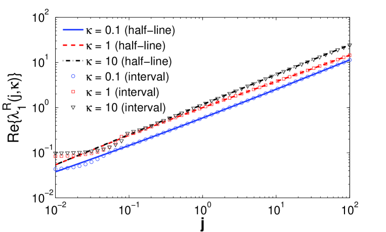
Figure 2: The graph of the real part of $\lambda_{1}^{R}({\mathfrak{j}},\kappa)$ as a function of ${\mathfrak{j}}$ for $\kappa=0.1$ (blue solid line and circles), $\kappa=1$ (red dashed line and squares), and $\kappa=10$ (black dash-dotted line and triangles). Lines show the numerical solution of (B.3), while symbols show $\inf{\rm Re\,}\sigma\big{(}\mathcal{L}^{R,D}({\mathfrak{j}},\kappa)\big{)}$.

We also present a numerical solution of (B.4) in Fig. 3 where we plot $\lambda_{1}^{R}$ as a function of $y=\kappa{\mathfrak{j}}^{-1/3}$. Note that, for any $y$, an eigenvalue of $\mathcal{L}^{R}(1,y)$ is the unique continuous solution of

$$ie^{i\,2\pi/3}\text{\rm Ai\,}^{\prime}(e^{i\,2\pi/3}\lambda(y))+y\,\text{\rm Ai\,}(e^{i\,2\pi/3}\lambda(y))=0\,,\,\lambda(0)=e^{-i\,2\pi/3}a^{\prime}_{n}\,,$$ (B.8)

where $a_{n}^{\prime}$ denotes the $n$-th zero of $\text{\rm Ai\,}^{\prime}$ starting from the right. We note this extension by $\widetilde{\lambda}_{n}^{R}(y)$ and we observe that $\widetilde{\lambda}_{n}^{R}(y)=\lambda_{n}^{R}(y)$ for $y\geq 0$ small enough by continuity. We will show at the end that this is true for any $y$. This notion is well defined since all the solutions of (B.8) are simple, as established in [19].

Considering in more detail the behavior of $\lambda_{1}^{R}(y)$, one expects that ${\rm Re\,}\{\lambda_{1}^{R}(y)\}$ monotonically grows from ${\rm Re\,}\{e^{-i2\pi/3}a^{\prime}_{1}\}\approx 0.5094$ (at $y=0$, corresponding to a Neumann condition [1]) to ${\rm Re\,}\{e^{-i2\pi/3}a_{1}\}\approx 1.1691$ (as $y\to+\infty$, corresponding to a Dirichlet condition [1]), where $a_{1}$ and $a^{\prime}_{1}$ are the rightmost zeros of Airy function and its derivative, i.e., ${\rm Re\,}(\lambda^{R}_{1})^{\prime}(y)>0\,$. This expected behavior is clearly manifested in Fig. 3.

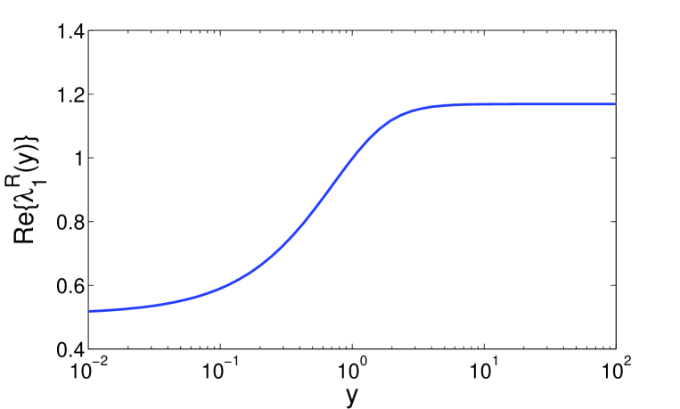
Figure 3: Robin case: the graph of the real part of $\lambda_{1}^{R}(y)$ obtained by numerical solution of (B.4).

Proof of Proposition B.1.

Let

$$\delta^{R}_{n}(y)=2-y\,\frac{{\rm Re\,}(\widetilde{\lambda}^{R}_{n})^{\prime}(y)}{{\rm Re\,}\widetilde{\lambda}_{n}^{R}(y)}\,,$$ (B.9)

By (B.7), it is sufficient to prove that

$$\delta^{R}_{n}(y)>0\,,\,\forall y\in[0,+\infty)\,,$$

in order to establish Proposition B.1. To this end, we first establish a differential equation for $\lambda_{n}^{R}(y)$. We set $\hat{\lambda}_{n}=e^{i\,2\pi/3}\widetilde{\lambda}^{R}_{n}$. We may represent (B.4) in the form

$$i\,e^{i\,2\pi/3}\text{\rm Ai\,}^{\prime}(\hat{\lambda}_{n}(y))+y\,\text{\rm Ai\,}(\hat{\lambda}_{n}(y))=0\,.$$ (B.10)

Differentiating with respect to $y$ yields, with the aid of Airy’s equation,

$$-i\,e^{i\,2\pi/3}\hat{\lambda}_{n}(y)\hat{\lambda}^{\prime}_{n}(y)-i\,e^{-i\,2\pi/3}\,y^{2}\hat{\lambda}^{\prime}_{n}(y)=1\,,$$

leading to the initial value problem, formulated for $\widetilde{\lambda}_{n}^{R}$,

$$\begin{cases}(\widetilde{\lambda}_{n}^{R})^{\prime}(y)(\widetilde{\lambda}_{n}^{R}(y)+y^{2})=-i\,,&\\ \widetilde{\lambda}_{n}^{R}(0)=e^{-i\,2\pi/3}a^{\prime}_{n}\,.&\end{cases}$$ (B.11)

We may now conclude that,

$$(\widetilde{\lambda}_{n}^{R})^{\prime}(0)=-i\,/\,\widetilde{\lambda}_{n}^{R}(0)\,.$$ (B.12)

Writing $u_{n}(y)={\rm Re\,}\{\widetilde{\lambda}_{n}^{R}(y)\}$ and $v_{n}(y)={\rm Im\,}\{\widetilde{\lambda}_{n}^{R}(y)\}$, one gets

$$\begin{split}u^{\prime}_{n}u_{n}-v^{\prime}_{n}v_{n}+u^{\prime}_{n}y^{2}&=0\,,\\ u^{\prime}_{n}v_{n}+v^{\prime}_{n}u_{n}+v^{\prime}_{n}y^{2}&=1\,,\\ \end{split}$$ (B.13)

from which we easily obtain that

$$u^{\prime}_{n}(y)=\frac{v_{n}(y)}{(u_{n}+y^{2})^{2}+v_{n}(y)^{2}}$$ (B.14)

and

$$v^{\prime}_{n}(y)=\frac{u_{n}(y)+y^{2}}{(u_{n}(y)+y^{2})^{2}+v_{n}(y)^{2}}>0\,.$$ (B.15)

As both $u_{n}$ and $v_{n}$ must be positive for all $y\in{\mathbb{R}}_{+}$ and $n\in\mathbb{N}^{*}$ (eigenvalues must belong to the numerical range), it easily follows that both $y\mapsto u_{n}(y)$ and $y\mapsto v_{n}(y)$ are monotone increasing for all $n\in\mathbb{N}$. In particular we have

$$\frac{1}{2}|a_{n}^{\prime}|=u_{n}(0)\leq u_{n}(y)\leq\lim_{y\to+\infty}u_{n}(y)=\frac{1}{2}|a_{\ell(n)}|\,,$$

for some $\ell(n)\in\mathbb{N}^{*}$.
But the same argument shows that each continuous (with respect to $y$) eigenvalue of $\mathcal{L}^{R}(1,y)$ is monotonous. This leads to a contradiction if $\ell(n)>n$. By recursion on $n$, we get that $\ell(n)=n$. Hence we have

$$-a^{\prime}_{n}<-a_{n}<-a^{\prime}_{n+1}\quad\forall n\in\mathbb{N}^{*}\,,$$

and we obtain that

$$u_{n}(y)<-a_{n}<u_{n+1}(y)\,,\quad\forall(y,n)\in{\mathbb{R}}_{+}\times\mathbb{N}^{*}\,,$$

and that $\widetilde{\lambda}_{n}^{R}(y)=\lambda_{n}^{R}(y)$ for all $y$ as expected.

We can now control the sign of $\delta^{R}_{n}(y)$, using the lower bound for $u_{n}$,

$$\frac{yu^{\prime}_{n}}{u_{n}}\leq\frac{yv_{n}}{u_{n}[2u_{n}y^{2}+v^{2}_{n}]}\leq\frac{1}{2^{\frac{3}{2}}u_{n}^{3/2}}\leq\frac{1}{2\sqrt{2}|a_{1}^{\prime}|^{3/2}}<2\,.$$ (B.16)

(cf. [1] for the justification of the last inequality.) The proposition now follows from (B.9) and (B.7).    

Remark B.2.

We may also obtain the asymptotic behavior of $\delta^{R}_{n}$ as $y\to+\infty$. As

$$\frac{yu^{\prime}_{n}(y)}{u_{n}(y)}\leq\frac{1}{2|a_{n}^{\prime}|\,y}\,\frac{2v_{1}(y)\,y^{2}}{y^{4}+v_{n}(y)^{2}}\leq\frac{1}{2|a_{n}^{\prime}|\,y}\,,$$ (B.17)

we obtain that

$$\lim_{y\to+\infty}\delta^{R}_{n}(y)=2\,.$$

In Fig. 4 we plot $yu_{1}^{\prime}(y)/u_{1}(y)$ as a function of $y$.

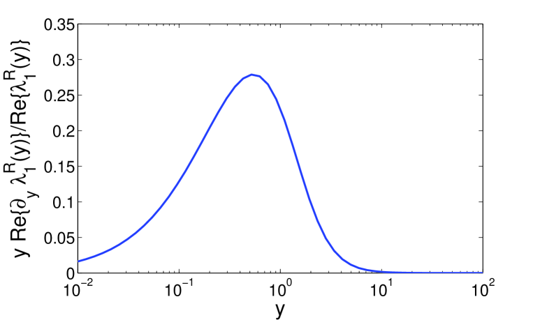
Figure 4: Robin case: the graph of $y\mapsto y\,{\rm Re\,}\{(\lambda^{R}_{1})^{\prime}(y)\}/{\rm Re\,}\{\lambda^{R}_{1}(y)\}$ obtained by a numerical solution of (B.4).

Alternatively, one can solve the problem on the interval $[0,L]$ with Robin and Dirichlet boundary conditions at $0$ and $L$ (with $L\gg 1$), respectively, using a Galerkin expansion, and then diagonalize the underlying matrix.

B.2 Transmission case

We consider the eigenvalues of the operator $\mathcal{L}^{T}({\mathfrak{j}},\kappa)=-\frac{d^{2}}{dx^{2}}+i{\mathfrak{j}}x$ on the line with transmission condition in (1.9) for a given non-negative value of $\kappa$. Introducing $\lambda^{T}=\lambda^{T}({\mathfrak{j}},\kappa)\,{\mathfrak{j}}^{-2/3}$, one gets the following equation

$$2\pi\text{\rm Ai\,}^{\prime}(e^{i2\pi/3}\lambda)\,\text{\rm Ai\,}^{\prime}(e^{-i2\pi/3}\lambda)=-\kappa\,{\mathfrak{j}}^{-1/3}.$$ (B.18)

Setting, as in the Robin case, $y=\kappa\,{\mathfrak{j}}^{-1/3}$ leads to

$$2\pi\text{\rm Ai\,}^{\prime}(e^{i2\pi/3}\lambda)\,\text{\rm Ai\,}^{\prime}(e^{-i2\pi/3}\lambda)=-y\,,$$ (B.19)

for $y\geq 0$.
This equation can be solved numerically to find $\lambda_{n}(\kappa{\mathfrak{j}}^{-1/3})$, from which we obtain the eigenvalues via the relation

$$\lambda_{n}^{T}({\mathfrak{j}},\kappa)={\mathfrak{j}}^{2/3}\,\lambda_{n}^{T}(\kappa\,{\mathfrak{j}}^{-1/3})\,.$$ (B.20)

Taking the derivative with respect to ${\mathfrak{j}}$ yields

$$\frac{\partial}{\partial{\mathfrak{j}}}{\rm Re\,}\lambda_{n}^{T}({\mathfrak{j}},\kappa)=\frac{{\rm Re\,}\lambda_{n}^{T}(\kappa\,{\mathfrak{j}}^{-1/3})}{3{\mathfrak{j}}^{1/3}}\biggl{(}2-\kappa\,{\mathfrak{j}}^{-1/3}\,\frac{({\rm Re\,}\lambda^{T}_{n})^{\prime}(\kappa\,{\mathfrak{j}}^{-1/3})}{{\rm Re\,}\lambda_{n}^{T}(\kappa\,{\mathfrak{j}}^{-1/3})}\biggr{)}\,.$$ (B.21)

We focus attention on the variation of ${\rm Re\,}\lambda_{1}^{T}({\mathfrak{j}},\kappa)$ with respect to ${\mathfrak{j}}$. To this end we attempt to determine the sign of

$$\delta^{T}(y)=2-y\,\frac{{\rm Re\,}(\lambda^{T}_{1})^{\prime}(y)}{{\rm Re\,}\lambda^{T}_{1}(y)}\,,$$ (B.22)

where $\lambda_{1}^{T}(y)$ is the unique continuous solution of (B.19) satisfying $\lambda_{1}^{T}(0)=|a_{1}^{\prime}|e^{i\pi/3}$.

Obviously, (B.19) poses a significantly greater obstacle than (B.4). The following simple observation can still be made:

Lemma B.3.

There exists $y_{0}>0$ such that $\delta^{T}(y)>0$ on $[0,y_{0}]$.

Proof.

By continuity, it is enough to prove the statement at $y=0$. By (B.22) and the fact that ${\rm Re\,}\lambda_{1}^{T}(0)=|a_{1}^{\prime}|/2>0$ we readily obtain $\delta^{T}(0)=2$.    

The following conjecture can be made in the large $y$ limit

Conjecture B.4.

There exists $y_{1}>0$ such that $\delta^{T}(y)>0$ on $[y_{1},+\infty)$.

Note that as $y\to+\infty$ the transmission problem “tends” to $-\frac{d^{2}}{dx^{2}}+ix$ on the line, which has no spectrum. Following [16], we provide in the sequel a formal justification for the conjecture together with an enlightening picture.

Figure 5 shows that the graph of $y\mapsto y\,\frac{{\rm Re\,}(\lambda^{T}_{1})^{\prime}(y)}{{\rm Re\,}\lambda_{1}^{T}(y)}$ attends its maximum at a value which is below $0.30$. As a consequence, by (B.6), ${\rm Re\,}\lambda_{1}^{T}$ is monotone increasing in ${\mathfrak{j}}$.

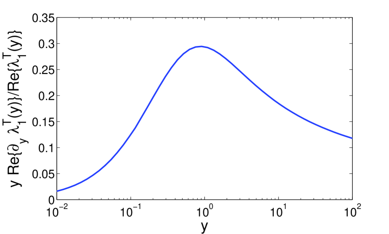
Figure 5: Transmission case: graph of $y\mapsto y\,{\rm Re\,}\{\partial_{y}\lambda_{1}^{T}(y)\}/{\rm Re\,}\{\lambda_{1}^{T}(y)\}$ obtained by numerical solution of (B.18).

B.2.1 Reminder on Airy functions

The Wronskian for Airy functions is

$$e^{-i2\pi/3}\text{\rm Ai\,}^{\prime}(e^{-i2\pi/3}z)\text{\rm Ai\,}(e^{i2\pi/3}z)-e^{i2\pi/3}\text{\rm Ai\,}^{\prime}(e^{i2\pi/3}z)\text{\rm Ai\,}(e^{-i2\pi/3}z)=\frac{i}{2\pi}\,\quad\forall~{}z\in\mathbb{C}\,.$$ (B.23)

Note that these two functions are related to $\text{\rm Ai\,}(z)$ by the identity

$$\text{\rm Ai\,}(z)+e^{-i2\pi/3}\text{\rm Ai\,}(e^{-i2\pi/3}z)+e^{i2\pi/3}\text{\rm Ai\,}(e^{i2\pi/3}z)=0\quad\forall~{}z\in\mathbb{C}\,.$$ (B.24)

By differentiation we also get

$$\text{\rm Ai\,}^{\prime}(z)+e^{i2\pi/3}\text{\rm Ai\,}^{\prime}(e^{-i2\pi/3}z)+e^{-i2\pi/3}\text{\rm Ai\,}^{\prime}(e^{i2\pi/3}z)=0\quad\forall~{}z\in\mathbb{C}\,.$$ (B.25)

The Airy function and its derivative satisfy different asymptotic expansions depending on their argument:
For $|\arg z|<\pi$,

$$\text{\rm Ai\,}(z) = \frac{1}{2}\pi^{-\frac{1}{2}}z^{-1/4}\,\exp\left(-\frac{2}{3}z^{3/2}\right)\bigl{(}1+\mathcal{O}(|z|^{-\frac{3}{2}})\bigr{)},$$ (B.26)

$$\text{\rm Ai\,}^{\prime}(z) = -\frac{1}{2}\pi^{-\frac{1}{2}}\,z^{1/4}\,\exp\left(-\frac{2}{3}z^{3/2}\right)\bigl{(}1+\mathcal{O}(|z|^{-\frac{3}{2}})\bigr{)}\,,$$ (B.27)

where moreover $\mathcal{O}$ is, for any $\epsilon>0$, uniform when $|\arg z|\leq\pi-\epsilon$ .

B.2.2 The behavior as $y\to+\infty$

The behavior of $\lambda_{1}^{T}(y)$ as $y\to+\infty$ (we choose the eigenvalue with positive imaginary part) was analyzed in [16] (in particular, see Fig. 1). Without full mathematical rigor, using in particular the asymptotics of the previous sub-subsection, it is established (see formula (40)) that

$${\rm Re\,}\lambda_{1}^{T}(y)\sim\biggl{(}\frac{3}{4}\log y\biggr{)}^{\frac{2}{3}}\mbox{ as }y\to+\infty\,.$$

and that

$$\lim_{y\to+\infty}{\rm Im\,}\lambda_{1}^{T}(y)=0\,.$$

With more effort, one can establish at least formally that

$${\rm Re\,}(\lambda_{1}^{T})^{\prime}(y)\sim\frac{1}{2}\,\frac{1}{y}\,\biggl{(}\frac{3}{4}\log y\biggr{)}^{-\frac{1}{3}}\,,$$

which confirms the monotonicity of ${\rm Re\,}\lambda_{1}^{T}$ for large $y$ and implies

$$\lim_{y\to+\infty}\delta^{T}(y)=2\,,$$

which confirms Conjecture B.4.
One can also formally obtain

$${\rm Im\,}\lambda_{1}^{T}(y)\sim\frac{\pi}{2}\,\biggl{(}\frac{3}{4}\log y\biggr{)}^{-\frac{1}{3}}\,.$$

References

- [1] M. Abramovitz and I. A. Stegun. Handbook of Mathematical Functions with Formulas, Graphs, and Mathematical Tables. United States Department of Commerce, National Bureau of Standards (NBS) (1964).
- [2] S. Agmon. Elliptic Boundary Value Problems. D. Van Nostrand Company, 1965.
- [3] Y. Almog. The stability of the normal state of superconductors in the presence of electric currents. SIAM J. Math. Anal. 40 (2) (2008), pp. 824-850.
- [4] Y. Almog and B. Helffer. On the spectrum of non-selfadjoint Schrödinger operators with compact resolvent. Comm. in PDE 40 (8) (2015), pp. 1441–1466.
- [5] Y. Almog, B. Helffer, and X.-B. Pan. Superconductivity near the normal state under the action of electric currents and induced magnetic fields in . Comm. Math. Phys. 300 (2010), pp. 147–184.
- [6] Y. Almog, B. Helffer, and X. Pan. Superconductivity near the normal state in a half-plane under the action of a perpendicular electric current and an induced magnetic field. Trans. AMS 365 (2013), pp. 1183-1217.
- [7] Y. Almog, B. Helffer, and X.-B. Pan. Superconductivity near the normal state in a half-plane under the action of a perpendicular electric current and an induced magnetic field II: The large conductivity limit. SIAM J. Math. Anal. 44 (2012), pp. 3671–3733.
- [8] Y. Almog and R. Henry. Spectral analysis of a complex Schrödinger operator in the semiclassical limit. SIAM J. Math. Anal. 44 (2016), pp. 2962–2993.
- [9] A. Aslanyan and E. B. Davies. Spectral instability for some Schrödinger operators. Numer. Math. 85 (2000), no. 4, 525–552.
- [10] K. Beauchard, B. Helffer, R. Henry, and L. Robbiano. Degenerate parabolic operators of Kolmogorov type with a geometric control condition. ESAIM: COCV 21 (2015), pp. 487–512.
- [11] E. B. Davies. Linear Operators and their Spectra, vol. 106 of Cambridge Studies in Advanced Mathematics, Cambridge University Press, Cambridge, 2007.
- [12] E. B. Davies. Pseudospectra, the harmonic oscillator and complex resonances. Proc. R. Soc. London A 455 (1999), pp. 585–599.
- [13] K.-J. Engel and R. Nagel. One-parameter Semigroups for Linear Evolution Equations, vol. 194 of Graduate Texts in Mathematics, Springer-Verlag, New York, 2000.
- [14] D. S. Grebenkov. NMR Survey of Reflected Brownian Motion. Rev. Mod. Phys. 79 (2007), pp. 1077–1137.
- [15] D. S. Grebenkov. Pulsed-gradient spin-echo monitoring of restricted diffusion in multilayered structures. J. Magn. Reson. 205 (2010), pp. 181-195.
- [16] D. S. Grebenkov. Exploring diffusion across permeable barriers at high gradients. II. Localization regime. J. Magn. Reson. 248 (2014), pp. 164–176.
- [17] D. S. Grebenkov, Diffusion MRI/NMR at high gradients: challenges and perspectives. (accepted to Micro. Meso. Mater., 2017).
- [18] D. S. Grebenkov, B. Helffer. On spectral properties of the Bloch-Torrey operator in two dimensions. Submitted. Preprint: http://arxiv.org/abs/1608.01925.
- [19] D. S. Grebenkov, B. Helffer, and R. Henry. The complex Airy operator with a semi-permeable barrier. To appear in SIAM J. Math. Anal (2017). Preprint: http://arxiv.org/abs/1603.06992.
- [20] B. Helffer. Spectral Theory and its Applications. Cambridge University Press (2013).
- [21] B. Helffer. On pseudo-spectral problems related to a time dependent model in superconductivity with electric current. Confluentes Math. 3 (2) (2011), pp. 237-251.
- [22] B. Helffer and A. Mohamed. Sur le spectre essentiel des opérateurs de Schrödinger avec champ magnétique. Ann. Inst. Fourier 38(2), pp. 95–113 (1988).
- [23] B. Helffer and F. Nier. Hypoelliptic estimates and spectral theory for Fokker-Planck operators and Witten Laplacians. Springer Lecture Note in Mathematics 1862 (2005).
- [24] B. Helffer and J. Nourrigat. Hypoellipticité Maximale pour des Opérateurs Polynômes de Champs de Vecteurs. Progress in Mathematics, Birkhäuser, Vol. 58 (1985).
- [25] R. Henry. Spectre et pseudospectre d’opérateurs non-autoadjoints. PhD thesis, Université Paris-Sud (2013).
- [26] R. Henry. On the semi-classical analysis of Schrödinger operators with purely imaginary electric potentials in a bounded domain. ArXiv:1405.6183 (2014).
- [27] M. Reed and B. Simon. Methods of Modern Mathematical Physics. Academic Press, New York, 4 volumes, 1972-1978.
- [28] A. A. Shkalikov, Spectral portraits of the Orr-Sommerfeld operator at large Reynolds numbers, Sovrem. Mat. Fundam. Napravl. 3 (2003), pp. 89–112.
- [29] J. Sjöstrand. Resolvent estimates for non-selfadjoint operators via semigroups. Around the research of Vladimir Maz’ya. III. Int. Math. Ser. 13, Springer, New York (2010), pp. 359-384.
- [30] S. D. Stoller, W. Happer, and F. J. Dyson. Transverse spin relaxation in inhomogeneous magnetic fields. Phys. Rev. A 44 (1991), pp. 7459-7477.
- [31] T. M. de Swiet and P. N. Sen. Decay of nuclear magnetization by bounded diffusion in a constant field gradient. J. Chem. Phys. 100 (1994), pp. 5597-5604.