Scaling characteristics of fractional diffusion processes in the presence of power-law distributed random noise

Abstract

We present results of the numerical simulations and the scaling characteristics of one-dimensional random fluctuations with heavy tailed probability distribution functions. Assuming that the distribution function of the random fluctuations obeys Lévy statistics with a power-law scaling exponent, we investigate the fractional diffusion equation in the presence of $\mu$-stable Lévy noise. We study the scaling properties of the global width and two point correlation functions, we then compare the analytical and numerical results for the growth exponent $\beta$ and the roughness exponent $\alpha$. ̵‌We also investigate the fractional Fokker-Planck equation for heavy-tailed random fluctuations. We show that the fractional diffusion processes in the presence of $\mu$-stable Lévy noise display special scaling properties in the probability distribution function (PDF). Finally, we study numerically the scaling properties of the heavy-tailed random fluctuations by using the diffusion entropy analysis. This method is based on the evaluation of the Shannon entropy of the PDF generated by the random fluctuations, rather than on the measurement of the global width of the process. We apply the diffusion entropy analysis to extract the growth exponent $\beta$ and to confirm the validity of our numerical analysis. The proposed fractional langevin equation can be used for modeling, analysis and characterization of experimental data, such as solar flare fluctuations, turbulent heat flow and etc.

I Introduction

In recent years, the study of systems displaying heavy-tailed distributions has attracted considerable attention including physical, chemical, biological, economical and geological systems sornette ; Jacobs ; Klages . Examples include, solar flare fluctuations Scafetta , the statistics of the turbulent fields sorriso ; biskamp and turbulent heat flow kadanoff , the global velocity of imbibition fronts planet2009 , density of a vibrated column of granular material Nowak , particle velocity fluctuations in granular system Radjai , front propagation in porous media Hansen2007 ; Asikainen2002 , propagation of cracks in solids alava2006statistical , crackling noise sethna2001crackling ; bonamy2008crackling and the motion of geological faults fisher1997statistics ; kawamura2012statistical , and many others.

The ability to summarize observations using a unified statistical model takes the great deal of interest of Physicists. One strategy for handling the unusual properties of the phenomenon addressed here is relying on the particle based models such as fractional Lévy motion, which includes power-law statistics and long-range correlations leading to non-Gaussian and non-local anomalous behaviors bovet2015r . In particular, fractional Lévy motion has been used to study suprathermal ions, created by fusion reaction bovet2014 , and turbulent plasmas bovet2015 , in vivo diffusion magnetic resonance imaging data fan2015 , solar power influx into the magnetosphere Schumann2012 , network traffic modeling Laskin2001 , solar wind fluctuations Watkin2005 and spatial variability in sedimentary rock formations Painter1994 .

We are particularly interested to understand these problems based on the investigation of the fluctuation dynamics on a macroscopic scale, which leading finally to random field associated with linear (or non-linear) stochastic partial differential equations. The propagation dynamics of random fluctuations, can be obtained by diffusion phenomena in the presence of random forcing functions. Theoretical modeling of diffusion processes in the presence of random fluctuations have been started with the famous work by Edwards and Wilkinson (EW) edwards-wilkinson . The EW model has found interesting applications in a wide range of non-equilibrium statistical physics, i.e. the interface dynamics surface2 ; nelsonbook . In the EW model, the scalar random field $h({x},t)$ evolving via the Langevin equation,

$$\frac{\partial h({x},t)}{\partial t}=D\nabla^{2}h({x},t)+\eta({x},t),$$ (1)

where $D$ is a constant related to the dynamical surface tension or diffusion, and $\eta({x},t)$ is assumed to be a Gaussian white noise which satisfies $\langle\eta({x},t)\rangle=0$ and $\langle\eta({x},t)\eta({x}^{\prime},t^{\prime})\rangle=2k_{B}T\delta({x}-{x}^{\prime})\delta(t-t^{\prime})$. Since the probability distribution function of the solution to Eq. (1), obeys a Gaussian law, it would be interesting to introduce a deformed version of EW model to investigate random fluctuations with heavy-tailed distributions.

A modified version of Eq. (1) was introduced by Lam and Sander lam1993exact . They suggested that one might describe the dynamics of the random fluctuations by a linear stochastic partial differential equation (1) in the presence of heavy-tailed noise. They answered how the statistics of height fluctuations, is affected by the presence of random noise with power-law distribution.

The fractional langevin equation governing the dynamics of non-local random fluctuations with heavy tailed distributions, recently proposed in Ref. nezhadhaghighi2017 . According to the scaling analysis approach, we have investigated the scaling characteristics of the fractional diffusion processes in the presence of $\mu$-stable Lévy noise.

In this work, our aim is to consider the same model in one spatial dimension and, based on the numerical simulations, to investigate the scaling properties of the heavy-tailed random fluctuations. Starting with Langevin equation (1) to describe the dynamics of Gaussian fluctuating interfaces, we systematically change the local diffusion operator by the non-local fractional operator. We also added heavy-tailed random processes to obtain a description applicable on the study of the correlated random fluctuations with power-law probability density functions. To this end, in Sec. II, we introduce our model and by means of scaling arguments we present the statistical properties of the model that is characterized by the $q$th order global width and $q$th order two point function. The existence of power-law behaviors, plus the assumption of the self-affine character of the heavy-tailed correlated random fluctuations allows us to obtain the scaling exponents of the process i.e. growth exponent and local (global) roughness exponent. Particular emphasis is put on the scaling characteristics of the probability distribution function (PDF). Using diffusion entropy analysis we show how the growth scaling exponent of the random fluctuation can be described by PDF dynamics. Sec. III, is devoted to the analysis of the fractional Fokker-Planck equation in order to drive the power-law scaling properties of the distributions. In Sec. IV, finite-difference numerical scheme is used to integrate stochastic fractional differential equation. In this section we summarize our numerical results. In Sec. V, we summarize the main findings and conclusions.

II Dynamics of heavy-tailed random fluctuations

In Eq. (1), the term $\nabla^{2}h({x},t)$ is proportional to the diffusion of the random fluctuation which is a local operator. In the general case we are interested to replace ordinary derivative with fractional one that is non-local fractional Laplacian. For this purpose, we define the fractional Langevin equation in the presence of heavy-tailed noise as,

$$\frac{\partial h({x},t)}{\partial t}=D_{z}\frac{\partial^{z}}{\partial|{x}|^{z}}h({x},t)+\eta_{\mu}({x},t),$$ (2)

so that for $z=2$ and $\mu=2$ we recover the standard EW model Eq. (1) (see Ref. nezhadhaghighi2017 ). In the above equation, the Laplacian operator has been replaced by $\frac{\partial^{z}}{\partial|{x}|^{z}}$, which is the fractional space derivative of order $z$. The fractional derivative is defined via its Fourier transform

$$\mathcal{F}\left\{\frac{\partial^{z}}{\partial|{x}|^{z}}h({x},t)\right\}\equiv-|\mathbf{q}|^{z}h(\mathbf{q},t),$$ (3)

where, $h(\mathbf{q},t)$ is Fourier transform of the random field $h({x},t)$. It is also possible to rewrite the fractional derivative in terms of the standard Laplacian $\mathop{}\!\mathbin{\bigtriangleup}$ as $\frac{\partial^{z}}{\partial|{x}|^{z}}\equiv-(\mathop{}\!\mathbin{\bigtriangleup})^{z/2}$ samko ; kilbas . The $\mu$-stable Lévy noise $\eta_{\mu}({x},t)$ is uncorrelated noise with power-law distribution function and $\langle\eta_{\mu}({x},t)\rangle=0$. The parameter $\mu>0$ characterizes the asymptotic power-law behavior of the stable distribution

$$p(x)\sim\frac{1}{|x|^{1+\mu}}.$$ (4)

We should note that the corresponding Lévy white noise with $0<\mu<2$, has infinite variance and the higher cumulants Klages ; stochastic book ; gardiner .

Here we are focusing on the scaling characteristics of Eq. (2) in one-dimension. It is easy to show that the solution to Eq. (2) is a self-affine random process. The scale transformation of space by factor $\lambda$ and of time by a factor $\lambda^{\nu}$ ($\nu$ is the dynamical scaling exponent), re-scales the random process $h(x,t)$ by factor $\lambda^{\alpha}$ as follows,

$$h(\lambda x,\lambda^{\nu}t)\equiv\lambda^{\alpha}h(x,t),$$ (5)

where $\alpha$ is called the roughness (Hurst) exponent. Therefore, the scale transformations of equation of motion for the random fields with heavy-tailed PDF, give us

$$\lambda^{\alpha-\nu}\frac{\partial h(x,t)}{\partial t}=\lambda^{\alpha-z}D_{z}\frac{\partial^{z}}{\partial|x|^{z}}h(x,t)+\lambda^{\gamma}\eta_{\mu}(x,t),$$ (6)

where $\gamma=(1+\nu)(1/\mu-1)$ (see Appendix A). The solution to Eq. (2), is scale invariant. Therefore, the values of the dynamical exponent $\nu$ as well as of the roughness exponent $\alpha$ depend on the fractional order $z$ and the asymptotic scaling power of the stable distribution $\mu$:

$$\nu=z\textrm{ and }\alpha=\frac{z+1}{\mu}-1.$$ (7)

Consider a random process $\eta_{\mu}(x,t)$ in Eq. (2) that is distributed with the probability density function Eq. (4). It implies that the variance, $\langle|\eta|^{2}\rangle$, is infinite. Most importantly, fractional moments $\langle|\eta|^{q}\rangle$ for all $q<\mu$, become finite. From this viewpoint it is evident that, the random fluctuations governed by fractional diffusion processes in the presence of heavy-tailed noise may be characterized by the $q$th order moments. In order to quantitatively characterize the fluctuation dynamics, let us first consider the $q$th order global width of the random field $h(x,t)$ defined by

$$w_{q}(t,L)\equiv\left\langle\overline{|h(x,t)-\overline{h(x,t)}|^{q}}\right\rangle^{1/q},$$ (8)

where the overline denotes a spatial average over the system of size $L$, and bracket denote ensemble averaging. For scale invariant random fluctuations, the global width satisfies the Family-Viscek scaling ansatz family85 and have asymptotic behavior given by

$$w_{q}(t,L)\sim\begin{cases}t^{\beta}&\quad t\ll t_{\times}\\ L^{\alpha_{g}}&\quad t\gg t_{\times}\\ \end{cases},$$ (9)

where $t_{\times}=L^{\nu}$ is the characteristic time and $\beta$ is called the growth exponent. The exponent $\alpha_{g}$ defines the so-called global roughness exponent. Self-affinity occurs when the $q$th order global width scales with a single $q$-independent exponent $\beta$. The scaling exponents $\alpha_{g}$, $\beta$ and $\nu$ are connected through the ratio $\beta=\alpha_{g}/\nu$, because of the self-affine scaling properties of the model under study surface2 .

To study the local properties of the fluctuating random field $h(x,t)$, the $q$th order two-point correlation function is defined as

$$C_{q}(r,t)\equiv\langle\left[h(x,t))-h(x^{\prime},0)\right]^{q}\rangle^{1/q}\sim r^{\alpha_{l}}f(rt^{-1/\nu}),$$ (10)

where the scaling function $f(u)$ behaves like

$$f(u)=\begin{cases}u^{-\alpha_{l}}&\quad u\gg 1\\ \text{const.}&\quad u\ll 1\\ \end{cases}.$$ (11)

where $r=|{x}-{x}^{\prime}|$. In the saturated regime ($t\gg L^{z}$), one expects $C_{q}$ to scale as $C_{q}(r)\sim r^{\alpha_{l}}$. The exponent $\alpha_{q}$’s define local roughness exponent. This exponent is another measure to distinguish between self-affine and multiscaling properties of the random fluctuations. For self-affine random fluctuations there is only one roughness exponent, and thus $\alpha_{g}=\alpha_{l}=\alpha$ for all $q$s surface2 .

The scale-invariance property in the fractional diffusion processes in the presence of $\mu$-stable Lévy noise can be described mathematically with the probability distribution function $\mathcal{P}[h(x,t)]$. It is the probability that the fluctuating non-equilibrium field in the position $x$ and time $t$ can take a specific value $h(x,t)$. Therefore, in order to investigate more precisely the scaling properties of $q$th order global width (9) and $q$th order two-point correlation function (10), it would be necessary to analyze and quantify the PDF of the process.

The Lagevin equation (2) is invariant under spatial translation $x\rightarrow x+x_{0}$ and scale transformations $x\rightarrow\lambda x$ and $t\rightarrow\lambda^{z}$. In spite of these symmetries, we expect the probability distribution function in this case to follow

$$\mathcal{P}[h(x,t)]\equiv\mathcal{P}(y=h|_{x=x_{0}},t,L)=\frac{1}{t^{\beta}L^{\alpha}}\mathcal{F}\left(\frac{y}{t^{\beta}},\frac{y}{L^{\alpha}}\right),$$ (12)

where in the early time, $t\ll L^{z}$, it takes the form

$$\lim_{t\to 0}\mathcal{P}(y,t)\equiv\mathcal{P}_{er}(y,t)=\frac{1}{t^{\beta}}\mathcal{G}_{1}\left(\frac{y}{t^{\beta}}\right),$$ (13)

and in long-time limit, $t\gg L^{z}$, Eq. (12) has the form

$$\lim_{t\to\infty}\mathcal{P}(y,t,L)\equiv\mathcal{P}_{st}(y,L)=\frac{1}{L^{\alpha}}\mathcal{G}_{2}\left(\frac{y}{L^{\alpha}}\right),$$ (14)

where $\mathcal{G}_{1}$ and $\mathcal{G}_{2}$ are universal functions. In the next section we carry out the asymptotic behavior $\mathcal{G}_{n}(x)\sim 1/x^{1+\mu}$.

According to Eq. (9), the $q$th order deviation of height from its mean behaves as:

$$w^{q}\equiv\int dy|y-\overline{y}|^{q}\mathcal{P}(y,t,L).$$ (15)

By taking into account that the fractional diffusion process (2) is invariant under $h\rightarrow-h$ (up/dawn symmetry), we immediately obtain $\mathcal{P}(y,t,L)=\mathcal{P}(-y,t,L)$. The symmetry in the PDF, corresponds to $\bar{h}=0$. To get the scaling form of Eq. (9), we have

$$w^{q}(t,L)\equiv 2\int_{0}^{\infty}dyy^{q}\mathcal{P}(y,t,L)=\begin{cases}I_{1}t^{q\beta}&\quad t\ll L^{z}\\ I_{2}L^{q\alpha}&\quad t\gg L^{z}\\ \end{cases},$$ (16)

where $I_{n}=2\int_{0}^{\infty}u^{q}\mathcal{G}_{n}(u)du$.

To get more complete description of the non-Gaussian probability distribution function of the process (2), it is instructive to calculate the diffusion entropy. This method of analysis is based on the Shannon entropy of the diffusion process information entropy . The Shannon entropy for the random field $h(x,t)$ can be defined as,

$$S(t)=-\int\mathcal{P}[h]\log\mathcal{P}[h]\mathcal{D}[h].$$ (17)

Let us suppose that $\mathcal{P}[h]$ fits the scaling condition of Eqs. (12) and (13). To show how the entropy analysis works, let us plug Eq. (13) into Eq. (17). After a simple algebra, we get:

$$S(t)=-\int\mathcal{G}_{1}(u)\log\mathcal{G}_{1}(u)du+\beta\log t$$ (18)

where the scaling exponent $\beta$ is the growth exponent. As a consequence, when the PDF has the scaling form of Eq. (13), the diffusion entropy grows log-linearly with time, $S(t)=\beta\log t+\mathrm{const}$. In addition the entropy, $S(t)=\mathrm{const}$, for the long time limit ($t\gg L^{z}$) and it depends on the system size.

III Fractional Fokker-Planck equation for heavy-tailed random fluctuations

The stochastic part $\eta_{\mu}(x,t)$ denotes a $\delta$-correlated, Lévy white noise which is composed of independent identical random variables that are distributed according to the stable density with the characteristic index $\mu$ ($0<\mu<2$); i.e. $P_{\mu}(x)$. The characteristic function $\phi(k)$ of a $\mu$-stable random variable $x$ can be represented by

$$\phi(k)\equiv\int_{-\infty}^{\infty}e^{-ikx}P_{\mu}(x)dx=e^{-c^{\mu}|k|^{\mu}}~{},$$ (19)

where $c$ is the scale factor Klages . From above definition it is obvious that the parameter choice $\mu=2$ yields the usual, Gaussian probability distribution $P_{2}(x)=(4\pi c^{2})^{-1/2}\exp(x^{2}/4c^{2})$ with the variance $\langle|x|^{2}\rangle=2c^{2}$. The closed form for the symmetric Lévy distribution when $\mu=1$ corresponds to the Cauchy distribution, $P_{1}(x)=\frac{c}{\pi(c^{2}+x^{2})}$. In general, all Lévy stable distributions $P_{\mu}(x)$ with $\mu<2$ follow the power-law asymptotic behavior

$$\lim_{x\rightarrow\infty}P_{\mu}(x)\equiv\frac{c^{\mu}\Gamma(1+\mu)\sin\pi\mu/2}{x^{1+\mu}}~{},$$ (20)

such that the variance is infinite and the fractional moments $\langle|x|^{q}\rangle$ are finite only for $q<\mu$ Jacobs . Note that the “tail” of Lévy densities are much wider than those of the Gaussian distribution Jacobs .

In order to characterize the probability distribution of the random fluctuations $h(x,t)$, we start from Eq. (23), and write the Langevin equation governing the dynamics of the Fourier components of the random field $h(k,t)=\int_{-\infty}^{\infty}e^{-ikx}h(x,t)dx$ which evolve according to

$$\dot{h}(k,t)=-D|k|^{z}h(k,t)+\eta_{\mu}(k,t)~{},$$ (21)

where $\eta_{\mu}(k,t)$ is power-law uncorrelated noise (in Fourier space) with the symmetric heavy-tailed distribution given in Eq. (20) at a particular time instant. For a fixed value of the Fourier mode $k$, it is convenient to discuss Eq. (21) in terms of the Langevin approach to Lévy flights in harmonic potential, such that

$$\dot{\mathcal{Q}}=f(\mathcal{Q})+\tilde{\eta}_{\mu}(t)~{},$$ (22)

where $\mathcal{Q}$ is the stochastic random process, $f(\mathcal{Q})=-D_{k}\mathcal{Q}$ is the harmonic force and $\tilde{\eta}_{\mu}(t)$ is the white Lévy stable noise. In many situations, one is interested in the probability distributions $\mathcal{P}(\mathcal{Q},t)\equiv\mathcal{P}(h,k,t)$ at some given time $t$. It can be shown that the kinetic equation for the probability distribution of the stochastic process $\mathcal{Q}$ has the form

$$\frac{\partial}{\partial t}\mathcal{P}(\mathcal{Q},t)=\left(-\frac{\partial}{\partial\mathcal{Q}}f(\mathcal{Q})+K_{\mu}\frac{\partial^{\mu}}{\partial|\mathcal{Q}|^{\mu}}\right)\mathcal{P}(\mathcal{Q},t)~{},$$ (23)

which is called space-fractional Fokker-Planck equation Klages . Stationary solution of the fractional diffusion equation Eq. (23) can be read from the asymptotic time independent solutions $\mathcal{P}_{st}(\mathcal{Q})=\lim_{t\rightarrow\infty}\mathcal{P}(\mathcal{Q},t)$. By analogy with the Ref. Chechkin2002 , the asymptotic limit ($\mathcal{Q}\rightarrow\infty$) of the stationary solution to the fractional Fokker-Planck equation (23) reads

$$\mathcal{P}_{st}(\mathcal{Q})=\frac{C_{\mu}}{D_{k}}\frac{1}{|\mathcal{Q}|^{1+\mu}}~{},$$ (24)

where $C_{\mu}=\frac{K_{\mu}\sin\pi\mu/2\Gamma(\mu)}{\pi}$ and $D_{k}=D|k|^{z}$. Thus, the stationary solution $\mathcal{P}_{st}(\mathcal{Q})\equiv\mathcal{P}_{st}(h,k)$ is a symmetric Lévy distribution, see Eqs. (20) and (24). Thus, we expect that the stationary probability distribution of the fluctuating field (with dynamics governed by a linear Langevin equation 2) is given by

$$\mathcal{P}_{st}(h)\propto 1/h^{1+\mu}.$$ (25)

It turns out, that the random field $h(x,t)$ given by the solution to Eq. (2) is clearly a correlated $\mu$-stable process (for $0<\mu<2$).

IV Numerical Results

Figure 1: (Color online) The $q$th order global width $w_{q}(t,L)$ with respects to time $t$ ($q=2/\mu$ for each case). For early times $t\ll L^{z}$, the $q$th order order global width scaled according to $w_{q}(t)\sim t^{\beta}$. Inset shows the scaling exponent (growth exponent) $\beta$ for different values of the fractional order $z$ and the stable parameter $\mu$. The solid red lines show the theoretical prediction $\beta=\frac{z+1}{z\mu}-\frac{1}{z}$.

Figure 2: (Color online) The $q$th order order global width $w_{q}(L)$ in the steady-state regime ($q=2/\mu$ for each case). Solid red line represents the scaling behavior $w_{q}(L)\sim L^{\alpha_{g}}$. Inset shows the scaling exponent (global roughness) $\alpha_{g}$ for different values of the fractional order $z$ and the stable parameter $\mu$. The solid red lines show the theoretical prediction $\alpha=\frac{z+1}{\mu}-1$.

In order to check the above predictions, this part is concerned with the numerical simulations of non-local diffusion equation in the presence of the $\mu$-stable Lévy noise for different fractional order $z$ and stable exponent $\mu$. To this end, we transform the Langevin equation (2) to discrete time and space. Consider the one-dimensional lattice of size $L$ and grid size $\Delta x$, with periodic boundary condition. We define $x=m\Delta x$ with $m=1,\dots,L$ and $t=n\Delta t$ with $n=0,1,\dots,N$, where $\Delta t$ is the time step.

The discretization of the Riesz-Feller derivative, can be efficiently generated by the matrix transform algorithm ilic2005numerical ; ilic2006numerical ; nezhadhaghighi2014 , which is,

$$\left.\frac{\partial^{z}}{\partial|x|^{z}}h(x,t)\right|_{(x=i\Delta x,t=n\Delta t)}\equiv\frac{1}{(\Delta x)^{z}}\sum_{j=1}^{L}\mathbb{K}_{i,j}h_{j}^{n}~{},$$ (26)

where the elements of the matrix $\mathbb{K}$, representing the discretized fractional operator, can be expressed as,

$$\mathbb{K}_{l,m}=\frac{\Gamma(-\frac{z}{2}+n)\Gamma(z+1)}{\pi\Gamma(1+\frac{z}{2}+n)}\sin(\frac{z}{2}\pi),$$ (27)

where $n=|l-m|$, and fractional order $z\geq 1$. If $z/2$ is an integer, then $\mathbb{K}(n)=(-1)^{z-n+1}C_{z,\frac{z}{2}+n}$ for $n\leq z/2$ and $\mathbb{K}(n)=0$ for $n>z/2$, where $C_{z,\frac{z}{2}+n}$ are binomial coefficients zoia2007fractional .

If the differential equation (2) is discretized in time using an explicit (Euler) method, besides Eq. (27), we obtain a finite difference approximations to the fractional diffusion equation, that is,

$$h_{i}^{n+1}=h_{i}^{n}+\frac{\Delta t}{(\Delta x)^{z}}\sum_{j=1}^{L}\mathbb{K}_{i,j}h_{j}^{n}+\Delta t^{1/\mu}\Delta x^{1/\mu-1}\zeta~{},$$ (28)

where $h_{i}^{n}$ approximates the random fluctuation $h(x,t)$ in terms of discrete space and time variables $x=i\Delta x$ and $t=n\Delta t$. In order to numerically generate the uncorrelated random noise $\eta(x,t)$ with heavy-tailed distribution, using the approximation discussed in Appendix. A, we used $\eta(x,t)\sim(\Delta x\Delta t)^{1/\mu-1}\zeta$ where $\zeta$ is independent identically random variable with distribution in the family (4).

Although the probability densities for almost all the $\mu$-stable processes have no known closed form, there is a simple and efficient method for numerically generating uncorrelated random numbers $\zeta$ with the symmetric Lévy distribution Jacobs . These are given by

$$\zeta=\frac{\sin(\mu V)}{\cos(V)^{1/\mu}}\left[\frac{\cos((1-\mu)V)}{W}\right]^{(1-\mu)/\mu},$$ (29)

where $V$ has a uniform density on the interval $(-\pi/2,\pi/2)$, and $W$ has the standard exponential distribution with mean $1$ weron .

Here, for sake of simplicity, the lattice constant $\Delta x$ has been set equal to one. The length of the time step, $\Delta t$, must be small enough (we choose $\Delta t=0.01$) to ensure the stability in Eq. (28). In order to determine scaling characteristics of the scalar field $h(x,t)$, we have simulated this model on a lattice of size $L\in{64,128,256,512,1024,2048}$, with flat initial condition ($h(x,0)=0$). All numerical measurements are made using an ensemble of $2\times 10^{4}$ realizations. As already mentioned earlier, in order to minimize finite-size effects, we impose periodic boundary conditions in such a way that for each elements of the matrix kernel $\mathbb{K}$, the relation $\mathbb{K}(n)=\mathbb{K}(n-L)$ occurs.

Figure 3: (Color online) The $q$th order correlation functions $C_{q}(r)$ in the saturated regime ( $q=2/\mu$ for each case). Solid red line represents the universal scaling behavior $C_{q}(r)\sim r^{\alpha_{l}}$. Inset shows the scaling exponent (local roughness) $\alpha_{l}$ for different values of the fractional order $z$ and the stable parameter $\mu$. The solid red lines show the theoretical prediction $\alpha=\frac{z+1}{\mu}-1$.

IV.1 Scaling exponents and self-affinity

We will now consider in detail the procedure for extracting the scaling exponents, $\beta$ and $\alpha_{g}$, from the $q$th order global width Eq. (9) and, $\alpha_{l}$ from the $q$th order two-point function Eq. (10).

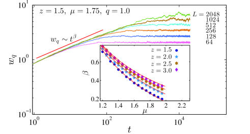
From the scaling properties the $q$th order global width, Eq. (9), we can measure growth exponent $\beta$. A plot of the global width $w_{q}$, with respect to time $t$, is given in Fig. (1) for various system size $L$. Through the relation $w_{q}\sim t^{\beta}$ for early times $t\ll L^{\nu}$, we obtain the exponent governing the rate of growth of the interface width. Since the log-log plot of $w_{q}$ is a linear function of time, we calculate $\beta$ as a function of stable parameter $\mu$ and fractional order $z$ in Fig. (1). Our numerical results agree well with the theoretical prediction $\beta=\frac{z+1}{z\mu}-\frac{1}{z}$.

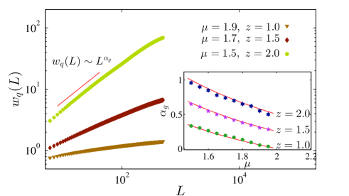
To determine the global roughness exponent $\alpha_{g}$ describing the saturation of the $q$th order global width, we use the relation $w_{q}\sim L^{\alpha_{g}}$ in the steady-state regime $t\gg L^{z}$. In Fig. (2) we show the scaling behavior of $q$th order global width $w_{q}$ with respect to the system size $L$ in the $\log-\log$ scale. In Fig. (2) we show $\alpha_{g}$ versus $\mu$ for different values of the fractional order $z$. The numerical simulation results were found to agree well with the analytical prediction $\alpha=\frac{z+1}{\mu}-1$.

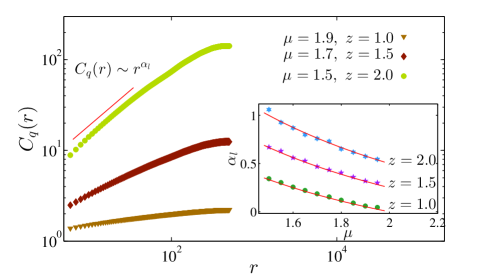
To check the validity of the scaling formulas derived in Sec. II, and to ensure the self-affinity of the correlated random fluctuations with heavy-tailed distributions, we have numerically evaluated the $q$th order two-point function Eq. (10). In the saturation regime, In Fig. (3) we show our numerical results for the correlation function $C_{q}$ scaled according to $C_{q}(r)\sim r^{\alpha_{l}}$ where $\alpha_{l}$ is the local roughness exponent. As shown in Fig. (3), we find excellent agreement between measured values of $\alpha_{l}$ with theoretical predictions $\alpha=\frac{z+1}{\mu}-1$. The self-affine scaling property of the heavy-tailed random fluctuation $h(x,t)$ obtained from $\alpha_{l}=\alpha$ for all $q$s.

IV.2 Heavy-tailed distribution function

Figure 4: (Color online) The probability distribution function $\mathcal{P}\{h,t\}$ for the random fluctuation $h$ in semi-log scale. The heavy-tailed random fluctuation $h(x,t)$ is the solution to the Eq. (2) with $z=1.5$ and $\mu=1.55$. (Inset) The same figure in $\log$-$\log$ scale shows this distribution is not Gaussian and it is distributed according to a power-law form $\mathcal{P}\{h\}\sim 1/h^{1+\mu}$.

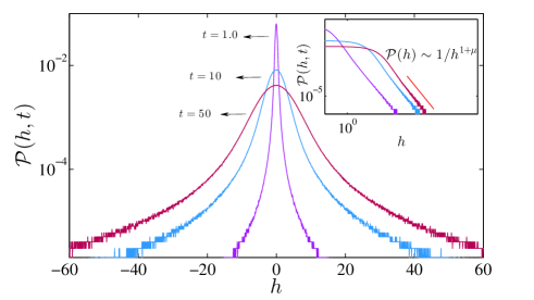
We now present the special properties of distribution function of the random fluctuation $h(x,t)$. As we saw earlier, probability distribution $\mathcal{P}(h,t,L)$ is essential for understanding the behavior of the dynamics of the process Eq. (2). Specifically, using Fourier component $\mathcal{Q}\equiv h(k,t)$, the time evolution of the corresponding probability distribution $\mathcal{P}(\mathcal{Q},t)$ is governed by the fractional Fokker-Planck equation (23). Therefore, we expect the stationary solution to the fractional Langevin equation (2) in the presence of the $\mu$-stable Lévy noise, to be distributed according to a power-law $\mathcal{P}(h)\sim{1/h^{1+\mu}}$. Fig. (4) shows $\mathcal{P}(h,t)$ as functions of $h$ for several times. These distributions are not Gaussian as indicated by the heavy-tails of the PDFs. These tails can be well approximated by power-law scaling behavior (25). So, in the saturation regime, $\mathcal{P}_{st}(h)$ increases linearly on a log-log plot, with the slope equal to $1+\mu^{\prime}$. We observe that the scaling factor $\mu^{\prime}$ behaves equal to the stable Lévy distribution index $\mu$.

IV.3 Diffusion entropy analysis

Figure 5: (Color online) Time evolution of diffusion entropy $S(t)$ for a numerical solution to Eq. (2). When the probability distribution is a power law in time (see Eq. (12)), the diffusion entropy increases linearly on a log-linear plot: $S(t)\sim\beta\log(t)$. Inset shows the scaling exponent (growth exponent) $\beta$ for different values of the fractional order $z$. The solid red lines show the theoretical prediction $\beta=\frac{z+1}{z\mu}-\frac{1}{z}$ (with $\mu=1.55$).

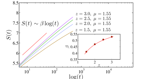
As a final characterization of the scaling behavior for the probability distribution $\mathcal{P}(h,t,L)$, we shall discuss here the special form of PDF: $\mathcal{P}(h,t,L)=\frac{1}{t^{\beta}L^{\alpha}}\mathcal{F}\left(\frac{h}{t^{\beta}},\frac{h}{L^{\alpha}}\right)$. As has been already shown, the early time dynamics of the probability distribution function, can be written in the scaling form of $\mathcal{P}_{er}(y,t)=\frac{1}{t^{\beta}}\mathcal{G}_{1}\left(\frac{y}{t^{\beta}}\right)$ (see Eq. 13). Very interestingly, when the scaling function is a power law in time, the diffusion entropy $S(t)=-\int dxp(x,t)\log p(x,t)$ provides an estimation for the scaling exponent $\beta$ which is exactly the same as the growth exponent. Figure (5) illustrates diffusion entropy analysis of the correlated random fluctuations with heavy-tailed distribution which exhibit the log-linear scaling property $S(t)\propto\beta\log t$. It is an interesting fact to stress here that the scaling exponent $\beta$ closely follows the theoretical prediction given by $\beta=\frac{z+1}{z\mu}-\frac{1}{z}$. In Fig. (5) the prefactor $\beta$ is plotted as a function of fractional order $z$.

V Conclusion

To summarize, we have studied the scaling properties of the random fluctuations with power-law distribution functions. By considering the non-local fractional operator and the $\mu$-stable Lévy noise, in a rather simple linear langevin equation (2), we have been able to characterize the statistical properties of non-Gaussian heavy-tailed random fluctuations. First, through scaling arguments we have shown that the solution to the fractional diffusion equation (2) obeys a simple scaling law, with a scaling exponent $\alpha$. We expect that the $q$-th order global moment and the $q$-th order correlation functions obey the power-law scaling. We derive analytic expressions for the local scaling exponents. We have also shown how the roughness exponent $\alpha$ and growth exponent $\beta$ can be analytically derived. We performed numerical simulations and measured these scaling exponents. Our numerical results are in perfect agreement with the analytical calculations, which supporting the numerical scheme developed herein. We also analyzed the scaling properties of the probability distribution functions and demonstrated the heavy-tailed distributions of the process by investigating the fractional Fokker-Planck equation for non-Gaussian heavy-tailed random fluctuations. We have shown that the probability distribution function for the solution to Eq. (2), even if the process is correlated in space and time, scales like $\mu$-stable Lévy processes. Based on the diffusion entropy analysis, we have studied the special scaling properties of the probability distribution functions, and we numerically calculated the growth scaling exponent $\beta$. The excellent agreement between the theoretical predictions and the numerical simulations provides a validation of our simulations. Finally, our study gives useful insights into the correlated random fluctuations with power-law PDFs, which makes it possible to establish the genuine nature of the related Physical phenomenons. This is left as a subject for further studies.

Appendix A Scaling properties of $\mu$-stable Lévy noise

Here, we discuss the scaling behavior of the symmetrical Lévy stable process $\eta_{\mu}(x,t)=\lambda^{-\gamma}\eta_{\mu}(\lambda x,\lambda^{\nu}t)$ under a scale transformation $x\rightarrow\lambda x$ and $t\rightarrow\lambda^{\nu}t$ lam1993exact . First consider a small region $\Omega=\Delta x\Delta t$ in ($x-t$) space, so we need to perform integration $I=\int_{\Omega}\eta_{\mu}(x,t)dxdt$. We can easily approximate it using the Monte Carlo method that numerically computes a definite integral. Thus, we could use the following procedure: (a) consider $N\sim\Delta x\Delta t$ random points on $\Omega$ with uniform distribution, (b) generate $N$ random numbers ${\xi_{i}}$ from power-law distribution $P(x)\sim 1/|x|^{1+\mu}$, (c) the integral $I$ can be approximated by

$$\int_{\Omega}\eta_{\mu}(x,t)dxdt=\sum_{i=1}^{N}\xi_{i}\sim N^{1/\mu}\xi.$$ (30)

where the latter approximation is obtained using the properties of the stable laws and the generalization of the central limit theorem stochastic book ; gardiner . This relation should be invariant under the scale transformation:

$$\lambda^{1+\nu}\int_{\Omega}\eta_{\mu}(\lambda x,\lambda^{z}t)dxdt\equiv\lambda^{(1+\nu)/\mu}N^{1/\mu}\xi.$$ (31)

which implies $\gamma=(1/\mu-1)(1+\nu)$ lam1993exact .

References

- (1) D. Sornette, Critical Phenomena in Natural Sciences: Chaos, Fractals, Selforganization and Disorder: Concepts and Tools, (Heidelberg, Germany: Springer-Verlag, 2000).
- (2) K. Jacobs, Stochastic processes for physicists: understanding noisy systems (Cambridge University Press, 2010).
- (3) R. Klages, G. Radons and I. M. Sokolov (Eds.) Anomalous transport: foundations and applications (John Wiley and Sons, 2008).
- (4) N. Scafetta and B. J. West, Phys. Rev. Lett., 90(24), (2003) 248701.
- (5) L. Sorriso-Valvo, V. Carbone, P. Veltri, H. Politano and A. Pouquet, EPL, 51(5) (2000) 520
- (6) D. Biskamp, and U. Bremer, Phys. Rev. Lett. 72.24 (1994) 3819
- (7) Leo P. Kadanoff, Physics today 54.8 (2001): 34-39.
- (8) R. Planet, S. Santucci and J. Ortín, Phys. Rev. Lett., 102.9 (2009) 094502
- (9) E. R. Nowak, A. Grushin, A. C. B. Barnum and M. B. Weissman, Phys. Rev. E, 63(2), (2001) 020301.
- (10) F. Radjai and S. Roux, Phys. Rev. Lett., 89(6), (2002) 064302.
- (11) A. Hansen, G. G. Batrouni, T. Ramstad and J. Schmittbuhl, (2007) Phys. Rev. E, 75(3), p.030102.
- (12) J. Asikainen, S. Majaniemi, M. Dubé and T. Ala-Nissila, (2002) Phys. Rev. E, 65(5), p.052104.
- (13) M. J. Alava, P. K. Nukala, and S. Zapperi, Advances in Physics, 55(3-4), 349-476 (2006).
- (14) J. P. Sethna, K. A. Dahmen and C. R. Myers, Nature, 410(6825), 242-250 (2001).
- (15) D. Bonamy, S. Santucci, and L. Ponson, Phys. Rev. Lett., 101(4), 045501 (2008).
- (16) D.S. Fisher, K. Dahmen, S. Ramanathan and Y. Ben-Zion, Phys. Rev. Lett. 78, 4885 (1997).
- (17) H. Kawamura, T. Hatano, N. Kato, S. Biswas and B. K. Chakrabarti, Reviews of Modern Physics, 84(2), 839 (2012).
- (18) A. Bovet, preprint: arXiv:1508.01879v1
- (19) A. Bovet, M. Gamarino, I. Furno, P. Ricci, a. Fasoli, K. Gustafson, D. E. Newman and R. Sánchez, Nuclear Fusion, 54(10), (2014) p.104009.
- (20) A. Bovet, A. Fasoli, P. Ricci, I. Furno and K. Gustafson, Phys. Rev. E, 91(4), (2015) p.041101.
- (21) Y. Fan and J-H Gao, Phys. Rev. E 92, (2015) 012707
- (22) A.Y. Schumann, N. R. Moloney and J. Davidsen, Extreme Events and Natural Hazards: The Complexity Perspective, (2012) pp.315-334.
- (23) N. Laskin, I. Lambadaris, F. C. Harmantzis and M. Devetsikiotis, Teletraffic Science and Engineering, 4, (2001) pp.457-470.
- (24) N. W. Watkins, D. Credgington, B. Hnat, S. C. Chapman, M. P. Freeman and J. Greenhough, Space science reviews, 121(1-4), (2005) pp.271-284.
- (25) S. Painter and L. Paterson, Geophysical Research Letters, 21(25), (1994) pp.2857-2860.
- (26) S. F. Edwards and D. R. Wilkinson, Proceedings of the Royal Society of London A: Mathematical, Physical and Engineering Sciences. Vol. 381. No. 1780. The Royal Society, (1982)
- (27) A. L. Barabśi and H. E. Stanley, Fractal Concepts in Surface Growth (Cambridge University Press, Cambridge, 1995)
- (28) D. Nelson, T. Piran, S. Weinberg, Statistical Mechanics of Membranes and Surfaces (World Scientific, 2004)
- (29) C. H. Lam and L. M. Sander,Phys. Rev. E 48.2 (1993) 979.
- (30) M. Ghasemi Nezhadhaghighi and A. Nakhlband, [arXiv:1703.07067] accepted for publication in: Phys. Rev. E (2017)
- (31) S. G. Samko, A. A. Kilbas and O. O. I. Marichev, Fractional integrals and derivatives (Gordon and Breach, New York, NY, 1993).
- (32) A. A. Kilbas, H. M. Srivastava, and J. J. Trujillo, Theory and Applications of Fractional Differential Equations, vol. 204 (Elsevier, 2006).
- (33) N. G. Van Kampen, Stochastic processes in physics and chemistry (Vol. 1. Elsevier, 1992)
- (34) C. W. Gardiner, Handbook of stochastic methods (Springer-Verlag, 1985)
- (35) F. Family and T. Viscek, J. Phys. A 18, L75 (1985).
- (36) N. Scafetta and P. Grigolini, Phys. Rev. E 66.3 (2002) 036130
- (37) A. V. Chechkin, V. Gonchar, J. Klafter, R. Metzler and L. Tanatarov, Chem. Phys. 284, (2002) 233–251.
- (38) M. Ilic, F. Liu, I. Turner, and V. Anh, Fractional Calcu- lus and Applied Analysis 8, 323p (2005).
- (39) M. Ilic, F. Liu, I. Turner, and V. Anh, Fractional Calcu- lus and Applied Analysis 9, 333p (2006).
- (40) M. Ghasemi Nezhadhaghighi, A. Chechkin and Ralf Metzler, The Journal of Chemical Physics 140.2 (2014): 024106.
- (41) A. Zoia, A. Rosso, and M. Kardar, Phys. Rev. E 76, 021116 (2007).
- (42) A. Janicki and A. Weron, Statistical Science, (1994) 109-126.