Computation of Ground States of the Gross-Pitaevskii Functional via Riemannian Optimization

Abstract

In this paper we combine concepts from Riemannian Optimization [P.-A. Absil, R. Mahony, R. Sepulchre, Optimization algorithms on matrix manifolds, Princeton University Press, 2008] and the theory of Sobolev gradients [J. W. Neuberger, Sobolev gradients, Springer 2010] to derive a new conjugate gradient method for direct minimization of the Gross-Pitaevskii energy functional with rotation. The conservation of the number of particles in the system constrains the minimizers to lie on a manifold corresponding to the unit $L^{2}$ norm. The idea developed here is to transform the original constrained optimization problem to an unconstrained problem on this (spherical) Riemannian manifold, so that fast minimization algorithms can be applied as alternatives to more standard constrained formulations. First, we obtain Sobolev gradients using an equivalent definition of an $H^{1}$ inner product which takes into account rotation. Then, the Riemannian gradient (RG) steepest descent method is derived based on projected gradients and retraction of an intermediate solution back to the constraint manifold. Finally, we use the concept of the Riemannian vector transport to propose a Riemannian conjugate gradient (RCG) method for this problem. It is derived at the continuous level based on the “optimize-then-discretize” paradigm instead of the usual “discretize-then-optimize” approach, as this ensures robustness of the method when adaptive mesh refinement is performed in computations. We evaluate various design choices inherent in the formulation of the method and conclude with recommendations concerning selection of the best options. Numerical tests carried out in the finite-element setting based on Lagrangian piecewise quadratic space discretization demonstrate that the proposed RCG method outperforms the simple gradient descent (RG) method in terms of rate of convergence. While on simple problems a Newton-type method implemented in the Ipopt library exhibits a faster convergence than the (RCG) approach, the two methods perform similarly on more complex problems requiring the use of mesh adaptation. At the same time the (RCG) approach has far fewer tunable parameters. Finally, the RCG method is extensively tested by computing complicated vortex configurations in rotating Bose-Einstein condensates, a task made challenging by large values of the non-linear interaction constant and the rotation rate as well as by strongly anisotropic trapping potentials.

68Q25, 68R10, 68U05

1 Introduction

The rotating Bose-Einstein condensate (BEC) represents a highly-controllable quantum system offering an ideal framework to study quantized vortices at a macroscopic level. A rich variety of vortex states, from a single vortex line to dense Abrikosov vortex lattices and giant vortices, were experimentally observed and extensively studied in the last two decades (e. g. [56]). A standard mathematical approach to describe equilibrium configurations with quantized vortices in rotating BEC is the minimization of the Gross-Pitaevskii (GP) energy functional with rotation [49, 42]. In addition to the global minima, the so-called “ground states”, local minima are also of interest as they represent excited, or meta-stable, states which are more likely to be observed in experiments [20]. The minimizers have the form of complex-valued wavefunction fields dependent on the space variable, resulting in an infinite-dimensional minimization problem. The complexity of the minimization problem is further compounded by a constraint imposed on the $L^{2}$ norm of the minimizers which reflects the conservation of the number of atoms in the condensate. For the mathematical properties of the GP energy with rotation and the corresponding ground states we refer the reader to [3, 6, 42, 15].

In this paper we address the problem of direct minimization of the GP energy functional with rotation when large nonlinear interaction constants and high rotation frequencies are considered. A number of approaches to direct minimization of the GP energy have been proposed based on various standard and emerging mathematical methods for optimization problems in finite dimension: Optimal Damping Algorithm [31, 38], Newton-like method based on Sequential Quadratic Programming (SQP) [21], Interior Point Method (Ipopt) [57], Inertial Proximal Algorithm (iPiano) [10] and regularized Newton method with trust region [60]. Alternative approaches which do not involve direct minimization of energy rely instead on the solution of the corresponding Euler-Lagrange system which has the form of a nonlinear eigenvalue problem. In the latter context, a wide variety of classical integration and iterative techniques have been employed such as Newton’s method [18], Runge-Kutta [22] and continuation methods [24], etc. We also mention the “deflated” Newton’s method, recently proposed in [25], which represents a systematic approach to determine several distinct solution branches.

Another class of approaches, pioneered in [16], relies on a normalized gradient flow for the GP functional and became popular due to their efficiency and ease of implementation (see also the review papers [13, 15, 9, 14]). These methods consist in first solving the gradient flow equation for the minimization of an unconstrained energy followed by a normalization of this “predictor” solution to bring it back to the constraint manifold. Solution of the gradient flow equation can be viewed as a pseudo-time (or imaginary time) integration of the time-independent GP equation. Discretization of the gradient-flow equations using a (natural) steepest descent method would result in a very inefficient explicit Euler scheme for the (imaginary-) time integration. For this reason in [16] the gradient-flow equation was solved using a semi-implicit backward Euler scheme which proved even more efficient than the classical Crank-Nicolson scheme. The convergence of the original scheme suggested in [16] was recently improved in [11, 12] by using different discrete preconditioners. It is interesting to note that the gradient-flow equation for the GP functional has structure similar to the complex-valued heat equation which makes it amenable to solution with different classical time-integration schemes such as Runge-Kutta-Fehlberg [34], backward Euler [16, 6, 17], second-order Strang time-splitting [16, 6], combined Runge-Kutta-Crank-Nicolson scheme [4, 5, 28], etc.

As regards the development of numerical methods, there are two main paradigms, namely, “optimize-then-discretize” and “discretize-then-optimize”, depending on whether the gradient expressions are derived at the continuous or discrete level. In the first case, the Sobolev gradient approach [45] represents the gradient-flow method formulated with respect to a judiciously selected inner product in a Hilbert space, rather than the classical $L^{2}$ inner product. The required gradients are obtained via the Riesz representation theorem. When discretized, the Sobolev gradient approach can be also interpreted as suitable preconditioning applied to the $L^{2}$ gradient [32]. However, the key advantage of working with the “optimize-then-discretize” formulation is that the form of this preconditioning is dictated by the functional (Sobolev) setting of the problem and thus avoids the technically complicated search for a good (and mesh-independent) discrete preconditioner. Sobolev gradient methods were successfully applied to minimize the GP energy in the presence of rotation in [34, 30].

The purpose of this contribution is to develop and validate an efficient computational approach to minimization of the GP energy by combining the Sobolev gradient method with concepts of Riemannian optimization [1, 54]. This allows us to transform the original constrained optimization problem to an unconstrained problem on a Riemannian manifold with a very simple structure which is amenable to solution using the conjugate gradient approach. We remark that while the “Riemannian structure” of an optimization problem may be exploited at various levels, in the present study we will focus solely on the basic concepts of “retraction” and “vector transport” describing how information travels along a manifold, and will not, in particular, consider endowing the constraint manifold with a Riemannian metric. In other words, we will assume that the constraint manifold is equipped with the metric induced by the embedding space. We begin by formulating a Riemannian version of the Sobolev gradient approach in which the retraction operation ensures that the norm constraint is satisfied at all discrete times. Then, convergence is accelerated using a Riemannian version of the conjugate gradient method which relies on the notion of the vector transport applied to the gradient and the descent direction. Such approaches are already well established in the context of problems formulated in finite dimensions [19], but have received only limited attention in the context of problems in infinite dimension. Convergence of the Riemannian versions of the BFGS quasi-Newton approach and of the Fletcher-Reeves conjugate gradients method was established in [51], whereas some applications were considered in [7, 48, 8, 44]. To the best of our knowledge, they represent a new direction as regards minimization of the GP energy. In our study, we carefully evaluate various design choices inherent in the formulation of the method and come up with recommendations concerning selection of the best options. Then, we demonstrate that in combination with a flexible finite-element discretization involving adaptive grid refinement [29, 57], the proposed approach outperforms a number of first-order techniques and performs on a par with a Newton-type method implemented in the Ipopt library [59].

The structure of the paper is as follows: in the next section we state the mathematical model describing minimization of the GP energy; in §3 we recall the Sobolev gradient method with its projected gradient variant, whereas the Riemannian gradient and conjugate gradient methods are introduced in §4; numerical discretization based on adaptive finite elements and its software implementation are discussed in §5; design choices to be explored in the formulation of the method are identified in §6; in §7 we use the method of the manufactured solutions to estimate the speeds of convergence of the different approaches; in §8 we compute a number of challenging BEC configurations with vortices in various arrangements; discussions and conclusions are deferred to §9.

2 Mathematical Model

The energy of a rotating homogeneous BEC at zero temperature is given in terms of the Gross-Pitaevskii (GP) energy functional [49, 42]. After applying standard scaling and dimension reduction [49, 15], its non-dimensional form defined here on a two-dimensional domain ${\mathcal{D}}\subset{\mathbb{R}}^{2}$ becomes

(1) $${E}(u)=\int_{{\mathcal{D}}}\left[\frac{1}{2}|\bm{\nabla}u|^{2}+C_{\text{trap}}\,|u|^{2}+\frac{1}{2}C_{g}|u|^{4}-iC_{\Omega}\,u^{*}{\bf A}^{t}\cdot\bm{\nabla}u\right]\,d{\mathbf{x}},$$

where $u\;:\ \;{\mathcal{D}}\rightarrow{\mathbb{C}}$ is a complex-valued wavefunction and $u^{*}$ its complex conjugate, ${\bf A}^{t}=(y,-x)$, $C_{\text{trap}}\;:\;{\mathcal{D}}\rightarrow{\mathbb{R}}$ is the trapping potential. $C_{g}$ and $C_{\Omega}$ are real constants characterizing the strength of the nonlinear interactions and rotation frequency, respectively. The wavefunction $u$ vanishes outside the trap and is therefore assumed to satisfy the homogeneous Dirichlet boundary conditions $u=0$ on $\partial{\mathcal{D}}$. The conservation of the number of atoms in the condensate is expressed as

(2) $$\|u\|_{2}:=\|u\|_{L^{2}({\cal D},{\mathbb{C}})}={\sqrt{\int_{{\mathcal{D}}}\left|u({\mathbf{x}})\right|^{2}\,d{\mathbf{x}}}}=1$$

and serves as a constraint on $u$. For the energy functional (1) to be well-defined, the wavefunction $u$ must belong to the Sobolev space $H_{0}^{1}({\mathcal{D}},{\mathbb{C}})$ of functions with square-integrable gradients [2] and vanishing traces on the boundary (precise definitions of the norms in this function space will be provided in §3 below). The constraint (2) may now be interpreted as defining a manifold ${\mathcal{M}}$ in the solution space, i. e.

(3) $${\cal M}:=\left\{u\in H^{1}_{0}({\cal D},{\mathbb{C}})\;:\;\|u\|_{2}=1\right\}.$$

We assume the trapping potential to have the following general form allowing us to represent different trapping potentials used in experiments

(4) $$C_{\text{trap}}(x,{y})=\frac{1}{2}\left(a_{x}x^{2}+a_{y}y^{2}+a_{4}r^{4}\right),\quad r^{2}=(x^{2}+y^{2}),$$

for some $a_{x},a_{y},a_{4}\in{\mathbb{R}}$. Along with the energy (1), another important integral quantity describing the rotating BEC is the total angular momentum

(5) $$L:={L}_{z}=i\int_{{\mathcal{D}}}u^{*}{\bf A}^{t}\cdot\bm{\nabla}u\,d{\mathbf{x}}$$

which under the assumed homogeneous Dirichlet boundary conditions is real-valued.

Global minimizers of the energy functional (1) defined through

(6) $$u_{g}=\arg\min_{u\in{\cal M}}E(u),\quad E(u_{g})<\infty,$$

are called ground states. Local minimizers, with energy larger than that of the ground state, are referred to as excited or meta-stable states. The Euler-Lagrange system corresponding to the minimization problem (6) is derived using standard techniques and leads to the stationary Gross-Pitaevskii equation

(7a) $$-\frac{1}{2}\nabla^{2}u+C_{\text{trap}}u+C_{g}|u|^{2}u-iC_{\Omega}{\bf A}^{t}\cdot\bm{\nabla}u = \,\,{\mu}\,u \text{in}\ {\mathcal{D}},$$

(7b) $$u = 0 \text{on}\ \partial{\mathcal{D}},$$

(7c) $${\|u\|_{2}} = 1$$ .

The ground state and excited states are therefore eigenfunctions of the nonlinear eigenvalue problem (7).

3 Gradient Flows and Steepest Descent Sobolev Gradient Methods

Numerical techniques for the solution of optimization problem (6) can be derived from a form of the gradient-flow equation which for practical reasons we state here in terms of the gradient of the energy functional (1) rather than the gradient of the corresponding Lagrangian functional

(8) $$\frac{du}{dt} =-\nabla_{{X}}E(u),\qquad t>0,$$

$$u(0) =u_{0},$$

where $u_{0}\in{\mathcal{M}}$ is an initial guess and $\nabla_{{X}}E(u)$ represents the gradient of the GP energy functional (1) at $u$, computed with respect to the topology of the Hilbert space ${X}$ (to be made specific below). The gradient flow needs to be additionally constrained to ensure that $u(t)\in{\mathcal{M}}$ for $t>0$. This approach is similar to the so-called normalized gradient-flow method [16], which first evolves (8) and then projects the intermediate solution back onto the manifold. It can be viewed as a splitting method for solving the continuous normalized gradient-flow equation [16] which is the constrained version of problem (8) in which the gradient $\nabla_{{X}}E(u)$ is replaced with the gradient of the corresponding Lagrangian.

As shown below, many different computational approaches can be derived from (8) by making specific choices of (i) the Hilbert space ${X}$, (ii) discretization of the initial-value problem (8) with respect to pseudo-time $t$ and (iii) how the constraint $u(t)\in{\mathcal{M}}$ is imposed.

As regards the expression of the gradient $\nabla_{{X}}E(u)$, it can be derived from the Gâteaux differential of energy (1) using the Riesz representation theorem [43] which depends on the choice of the inner-product space $X$. Since energy (1) is a twice continuously differentiable function from $H_{0}^{1}({\mathcal{D}},{\mathbb{C}})$ to ${\mathbb{R}}$, a natural choice for the inner product that will ensure the existence of a gradient is

(9) $${\langle u,v\rangle}_{H^{1}}=\int_{\mathcal{D}}{(u,v)+(\bm{\nabla}u,\bm{\nabla}v)}\,d{\bf x},$$

where $(u,v)=uv^{*}$ is the complex (${\mathds{C}}$ or ${\mathds{C}}^{2}$) inner product. A new inner product equivalent (in the precise sense of norm equivalence) to (9) was suggested in [30]

(10) $${\langle u,v\rangle}_{H_{A}}=\int_{\mathcal{D}}{(u,v)+(\bm{\nabla}_{A}u,\bm{\nabla}_{A}v)}\,d{\bf x},\quad\bm{\nabla}_{A}=\bm{\nabla}+iC_{\Omega}{\bf A},$$

and will be adopted in our considerations below. Its definition was motivated by the following physically more revealing form of the energy functional equivalent to (1)

(11) $${E}(u)=\int_{\cal D}\left[\frac{1}{2}\left|\bm{\nabla}u+iC_{\Omega}\,{\bf A}u\right|^{2}+C^{\text{eff}}_{\text{trap}}\,|u|^{2}+\frac{1}{2}C_{g}|u|^{4}\right]\,d{\mathbf{x}},$$

where the effective non-dimensional trapping potential $C^{\text{eff}}_{\text{trap}}$ is obtained from the original potential by subtracting a term representing the centrifugal force [55]

(12) $$C^{\text{eff}}_{\text{trap}}(x,y)=C_{\text{trap}}(x,y)-\frac{1}{2}C_{\Omega}^{2}\,r^{2}.$$

We add that, since the solution space $H^{1}_{0}({\mathcal{D}},{\mathbb{C}})$ is a subspace of both $H^{1}({\mathcal{D}},{\mathbb{C}})$ and $H_{A}({\mathcal{D}},{\mathbb{C}})$, we will assume $H^{1}_{0}({\mathcal{D}},{\mathbb{C}})$ to be equipped with the inner product (9) or (10), and the notation $X=H^{1}$ or $X=H_{A}$ will make it clear which one is used.

For each $u\in X$, one can find an element of $X$ denoted $\nabla_{X}E(u)$, such that the directional Gâteaux derivative of the energy at $u$ in the direction $v$, which is a continuous linear functional from ${X}$ to ${\mathbb{R}}$, is expressed as

(13) $$E^{\prime}(u)v=\Re\left(\langle\nabla_{X}E(u),v\rangle_{X}\right),\quad\forall v\in X,$$

where $\Re(\cdot)$ denotes the real part of a complex number. We refer to such an element of $X$ as the gradient of $E$ at $u$. Computing the Gâteaux derivative of the energy functional (1), we obtain

(14) $$E^{\prime}(u)v=2\Re\left(\int_{\mathcal{D}}\left[\frac{1}{2}(\bm{\nabla}u,\bm{\nabla}v)+\left(C_{\text{trap}}u+C_{g}\lvert u\rvert^{2}u-iC_{\Omega}{\bf A}^{t}\cdot\bm{\nabla}u,v\right)\right]\,d{\mathbf{x}}\right)$$

which, together with (13), allows us to identify the gradient $\nabla_{X}E(u)$. In particular, the $H_{A}$ gradient, hereafter denoted $G=\nabla_{H_{A}}E(u)$, will be computed by solving the elliptic boundary-value problem resulting from (14), (13) and (10), which we state here in the equivalent weak form

(15) $${\forall v\in{H_{0}^{1}({\mathcal{D}},{\mathds{R}})}},\int_{\mathcal{D}}\left[\left(1+C_{\Omega}^{2}(x^{2}+y^{2})\right)(G,v)+(\bm{\nabla}G,\bm{\nabla}v)-2iC_{\Omega}({\bf A}^{t}\cdot\bm{\nabla}G,v)\right]\,d{\mathbf{x}}\\ =2\int_{\mathcal{D}}\left[\frac{1}{2}(\bm{\nabla}u,\bm{\nabla}v)+\left(C_{\text{trap}}u+C_{g}\lvert u\rvert^{2}u-iC_{\Omega}{\bf A}^{t}\cdot\bm{\nabla}u,v\right)\right]\,d{\mathbf{x}}.$$

3.1 Normalized gradient flow

We note from (13) and (14) that, in order for $E^{\prime}(u)$ to be bounded in the $L^{2}({\mathcal{D}},{\mathbb{C}})$ norm, stronger regularity assumptions must be imposed on the solution $u$, namely $u\in H^{2}({\mathcal{D}},{\mathbb{C}})$. In this case, from (14) we obtain that

(16) $$E^{\prime}(u)v=2\Re\left(\int_{\mathcal{D}}\left({-\frac{1}{2}}\nabla^{2}u+C_{\text{trap}}u+C_{g}\lvert u\rvert^{2}u-iC_{\Omega}{\bf A}^{t}\cdot\bm{\nabla}u,v\right)\,d{\mathbf{x}}\right),$$

which allows us to formally derive a ”$L^{2}$-gradient” corresponding to the $L^{2}$ inner product

(17) $${\langle u,v\rangle}_{L^{2}}=\int_{\mathcal{D}}(u,v)\,d{\bf x}.$$

We add that this is the expression appearing on the left-hand side of the Euler-Lagrange equation (7a). The gradient flow equation (8) with this $L^{2}$-gradient was discretized in [16] using a semi-implicit backward Euler (BE) method

(18) $$\frac{{\tilde{u}}-u_{n}}{\delta t}=\frac{1}{2}\nabla^{2}{\tilde{u}}-C_{\text{trap}}{\tilde{u}}-C_{g}|u_{n}|^{2}{\tilde{u}}+iC_{\Omega}{\bf A}^{t}\cdot\bm{\nabla}{\tilde{u}},$$

where $u_{n}=u(t_{n})$ denotes the approximation obtained at the $n$th discrete time level, $\tilde{u}=\tilde{u}(t_{n+1})$ is an intermediate (predictor) field and $\delta t$ is a fixed (pseudo-)time step. The approximation $u_{n+1}$ at the time level $t_{n+1}$ has to satisfy the unit-norm constraint (2) and is therefore obtained by normalizing the predictor solution as

(19) $$u_{n+1}=\frac{{\tilde{u}}(t_{n+1})}{\|{\tilde{u}}(t_{n+1})\|_{2}}.$$

This approach is referred to as the normalized gradient flow method (see also [13, 15, 9, 14]). Different existing variants of this method use various numerical approaches to integrate the gradient-flow equation (8), e. g. Runge-Kutta methods [34, 4, 5, 28], different implicit schemes [16, 6, 17] and Strang-type time-splitting approaches [16, 6]. Even though some of these schemes do possess the energy-decreasing property, they typically do not preserve the gradient-flow structure at the discrete level, in the sense that the expression on the right-hand side (RHS) of the gradient-flow equation (8) discretized with respect to the pseudo-time $t$ is no longer in the form of a gradient of $E(u)$ (this is because, as a result of the hybrid explicit/implicit treatment, different terms in this expression may depend on the state $u$ approximated at different time levels, as happens in (18)). Therefore, such imaginary-time methods can be regarded as solving the nonlinear eigenvalue problem (7), rather than directly minimizing the GP energy. Another potential drawback of such approaches is that solutions of (7) are in general critical points of the energy which are not necessarily minima.

3.2 Steepest Descent Sobolev Gradient Methods

Hereafter we focus on techniques which do preserve the gradient-flow structure of (8) on the discrete level while explicitly accounting for the presence of the unit-norm constraint (2). As a starting point, we will thus consider an explicit discretization of (8) in the following generic form

(20) $$u_{n+1}=u_{n}-\tau_{n}\,G_{n},\quad n=0,1,\dots,$$

where $\tau_{n}$ is a suitable descent step size, whereas $G_{n}=G(u_{n})=\nabla_{X}E(u_{n})$ is a Sobolev gradient defined for ${X}=H_{A}$ or $H^{1}$. Below we discuss two ways in which the information about the constraint $u\in{\mathcal{M}}$ can be incorporated in the gradient method.

3.2.1 Projected Sobolev Gradient Method

By considering the following identity derived from (20)

(21) $$\|u_{n+1}\|_{2}^{2}=\|u_{n}-\tau_{n}\,G_{n}\|_{2}^{2}=\|u_{n}\|_{2}^{2}-2\tau_{n}\Re\langle u_{n},G_{n}\rangle_{L^{2}}+\tau_{n}^{2}\|G_{n}\|_{2}^{2},$$

we note that using an unconstrained gradient $G_{n}$ leads to an $\mathcal{O}(\tau_{n})$ error in the satisfaction of the constraint (2) at each iteration. Normalization of the solution is then necessary to bring it back onto the manifold $\cal M$ (see Figure 1a).

Figure 1: Schematic illustration of the principle of the steepest descent method on the spherical manifold $\cal M$ for (a) the simple (“unprojected”) gradient method and (b) the projected gradient (PG) and the Riemannian gradient (RG) methods. In case (b), since the projected gradient $P_{u_{n},H_{A}}G_{n}$ belongs to the subspace ${\cal T}_{u_{n}}{\cal M}$ tangent to the manifold at $u_{n}$, normalization is equivalent to Riemannian retraction (27).

This error can be reduced to second order $\mathcal{O}(\tau_{n}^{2})$ by requiring that $\langle u_{n},G_{n}\rangle_{L^{2}}=0$, which is achieved by projecting the gradient $G_{n}$ onto the subspace

(22) $${\cal T}_{u_{n}}{\cal M}=\left\{v\in H_{0}^{1}({\mathcal{D}},{\mathbb{C}})\;:\;\langle u_{n},v\rangle_{L^{2}}=0\right\}$$

tangent to the constraint manifold $\cal M$ at $u_{n}$. As was shown in [30, 41], the associated projection operator $P_{u_{n},{X}}$ can be expressed in the following general form

(23) $$P_{u_{n},{X}}G_{n}=G_{n}-\lambda\,v_{{X}},\qquad\lambda=\frac{\Re\langle u_{n},G_{n}\rangle_{L^{2}}}{\Re\langle u_{n},v_{{X}}\rangle_{L^{2}}},$$

where $v_{{X}}$ is a solution of the variational problem

(24) $$\langle v_{{X}},v\rangle_{{X}}=\langle u_{n},v\rangle_{L^{2}},\quad\forall v\in{{X}}.$$

We note that if $X=L^{2}$, $v_{X}=u$ in (24) and we recover the well-known explicit expression of the projected $L^{2}$-gradient (e. g. [7]).

Hereafter we will set ${X}=H_{A}$ and denote $G_{n}=\nabla_{H_{A}}E(u_{n})$. Replacing $G_{n}$ with $P_{u_{n},H_{A}}G_{n}$ in (20), we obtain the projected gradient (PG) method suggested in [30]

(25) $$\text{(PG)}\qquad u_{n+1}=u_{n}-\tau_{n}\ P_{u_{n},H_{A}}G_{n},\quad n=0,1,\dots,$$

While in [30] a fixed step size $\tau_{n}=\tau>0$ was used, here we use an optimal step size found through the solution of a line-minimization problem

(26) $$\tau_{n}=\mathop{argmin}_{\tau>0}\,E\left(u_{n}-\tau\,P_{u_{n},H_{A}}G_{n}\right).$$

An explicit expression for the optimal descent step was derived in [57] based on a particular form of the GP energy. In this study, we prefer to solve problem (26) with a general line-minimization approach such as Brent’s algorithm [50, 46] as it has the advantage of being easily adapted to the Riemannian gradient methods presented in the next section. To mitigate the $\mathcal{O}(\tau_{n}^{2})$ drift away from the constraint manifold ${\mathcal{M}}$ allowed by the (PG) iterations, normalization analogous to (19) may be applied to the iterates $u_{n}$ after a certain number of steps. The idea of the (PG) approach is illustrated schematically in Figure 1b.

4 Riemannian Optimization

In this section we discuss some basic concepts relevant to optimization on manifolds, known as Riemannian optimization [1, 54]. In contrast to the perspective developed in the previous section, here we pursue a different, “intrinsic” approach where optimization is performed directly on the manifold $\cal M$. The main advantage of such a formulation is that it allows one to treat (6) as an unconstrained optimization problem creating an opportunity to apply a suitable modification of the conjugate gradient method as an alternative to more traditional constrained approaches such as, e. g. Sequential Quadratic Programming (SQP) for nonlinear optimization.

In addition to the definition of the projection on the tangent space ${\cal T}_{u}{\cal M}$ already introduced above, cf. (23)–(24), we need to introduce two more concepts, namely, the “retraction” (also referred to as “exponential mapping”) and the associated “vector transport”. While in general these operators can have a rather complicated form, in the present problem where the constraint manifold $\cal M$ is given by (3), they can be reduced to fairly simple expressions. We refer the reader to the monograph [1] for additional details concerning the differential–geometry foundations of this approach.

4.1 Riemannian Gradient Method

Given a tangent vector $\xi\in{\cal T}_{u}{\cal M}$, where $u\in{\cal M}$ is a state on the manifold, the retraction ${{\cal R}}_{u}\;:\;{\cal T}_{u}{\cal M}\rightarrow{\cal M}$ is defined as the operator

(27) $${{\cal R}}_{u}(\xi)=\frac{u+\xi}{\|u+\xi\|_{2}},$$

where the norm used in the denominator is the same as the norm defining the constraint manifold in (3). We note that for the spherical manifold ${\mathcal{M}}$ the retraction operator is equivalent to normalization (19) already used in the previous sections.

The Riemannian gradient (RG) method is then obtained applying relation (27) to the projected gradient $P_{u_{n},H_{A}}G_{n}$, cf. (23)–(24), used in the (PG) approach which yields

(28) $$\text{(RG)}\qquad u_{n+1}={{\cal R}}_{u_{n}}\left(-\tau_{n}P_{u_{n},H_{A}}G_{n}\right),\qquad n=0,1,\dots.$$

The step size $\tau_{n}$ is found optimally by solving a generalization of the line-minimization problem (26) which uses retraction (27) to constrain the samples to manifold ${\mathcal{M}}$, i. e.

(29) $$\tau_{n}=\mathop{argmin}_{\tau>0}E\left({{\cal R}}_{u_{n}}(-\tau P_{u_{n},H_{A}}G_{n})\right).$$

We refer to problem (29) as “arc-minimization”. It is solved using a straightforward modification of Brent’s algorithm [50, 46]. In addition to application of retraction (27) at every iteration in the latter case, the key difference between the (PG) and (RG) approaches lies in how the optimal step size $\tau_{n}$ is determined, cf. (26) vs. (29). The idea of the (RG) method is illustrated schematically in Figure 1b.

4.2 Riemannian Conjugate Gradient Method

As a point of reference, we begin by recalling the nonlinear conjugate gradients method in the Euclidean case. Given a function $f\;:\;{\mathds{R}}^{N}\rightarrow{\mathds{R}}$, this approach finds its local minimum $\overline{{\bf u}}$ as $\overline{{\bf u}}=\lim_{n\rightarrow\infty}{\bf u}_{n}$, with the iterates ${\bf u}_{n}$ defined as follows [46]

(30) $${\bf u}_{n+1}={\bf u}_{n}+\tau_{n}\,{\bf d}_{n},\qquad n=0,1,\dots,$$

where ${\bf u}_{0}$ is the initial guess and the descent direction ${\bf d}_{n}$ is constructed as

(31) $${\bf d}_{0} =-{\bf g}_{0},$$

$${\bf d}_{n} =-{\bf g}_{n}+\beta_{n}\,{\bf d}_{n-1},\qquad n=1,2,\dots$$

in which ${\bf g}_{n}=\bm{\nabla}f({\bf u}_{n})$ and $\beta_{n}$ is a “momentum” term chosen to enforce the conjugacy of the search directions ${\bf d}_{k}$, $k=1,\dots,n$. When the objective function is convex-quadratic, i. e. $f({\bf u})={\bf u}^{T}{\bf A}{\bf u}$ for some positive-definite matrix ${\bf A}\in{\mathds{R}}^{N\times N}$, approach (30)–(31) reduces to the “linear” conjugate gradient method in which $\tau_{n}$ and $\beta_{n}$ are given in terms of simple expressions involving ${\bf A}$ [46]. In the non-quadratic setting, which is the case of problem (6), the step size $\tau_{n}$ needs to be found via line minimization as described by (29), whereas the momentum term is typically computed using one of the following expressions

(32a) $$\beta_{n} =\beta_{n}^{FR}:=\frac{\langle{\bf g}_{n},{\bf g}_{n}\rangle_{{\cal Y}}}{\langle{\bf g}_{n-1},{\bf g}_{n-1}\rangle_{{\cal Y}}} \text{(Fletcher-Reeves)},$$

(32b) $$\beta_{n} =\beta_{n}^{PR}:=\frac{\langle{\bf g}_{n},({\bf g}_{n}-{\bf g}_{n-1})\rangle_{{\cal Y}}}{\langle{\bf g}_{n-1},{\bf g}_{n-1}\rangle_{{\cal Y}}} \text{(Polak-Ribi{\`{e}}re)},$$

where $\langle\cdot,\cdot\rangle_{{\cal Y}}$ is the inner product defined with respect to the metric $\cal Y$ (in the simplest case when ${\bf u}\in{\mathds{R}}^{N}$, $\langle{\bf{a}},{\bf{b}}\rangle_{{\cal Y}}={\bf{a}}^{T}{\bf{b}}$ for ${\bf{a}},{\bf{b}}\in{\mathds{R}}^{N}$). The coefficient $\beta_{n}$ may be periodically reset to zero which is known to improve convergence for convex, non-quadratic problems [46]. It is well known that for optimization problems which are locally quadratic the conjugate gradient approach exhibits faster (though still linear) convergence than the convergence characterizing the simple gradient method, especially for poorly scaled problems [46]. Similar observations have been also reported for Riemannian optimization problems [1, 54].

We explain below how the conjugate gradients approach can be adapted to the Riemannian case involving the energy functional (1) defined for infinite-dimensional state variables $u\in H_{0}^{1}({\cal D})$. There are two key issues which must be addressed:

1. the two terms on the RHS of formula (31) belong to two different linear spaces which are the tangent spaces constructed at two consecutive iterations, i. e. ${\bf g}_{n}\in{\cal T}_{{\bf u}_{n}}{\cal M}$ and ${\bf d}_{n-1}\in{\cal T}_{{\bf u}_{n-1}}{\cal M}$; as a result, they cannot be simply added; the same problem also concerns the inner-product expressions in the numerator of the Polak-Ribière momentum term (32b),

2. while in the finite dimensions all norms are equivalent, this is no longer the case in the infinite-dimensional setting where the choice of the metric does play a significant role; in our approach, although the gradient-descent equations are discretized in space for the purpose of the numerical solution, their specific form is derived in the infinite-dimensional setting (in other words, we follow the “optimize-then-discretize” paradigm [35]); in addition to the momentum term (32), the choice of the metric implied by the inner product also plays a role in the construction of the projection (23)–(24) and the vector transport which will be defined below.

The key concept required in order to address the first issue is the vector transport

(33) $${{\cal TM}\oplus{\cal TM}\rightarrow{\cal TM}\;:\;(\eta,\xi)\longmapsto{\mathcal{T}}_{\eta}(\xi)\in{\cal TM},}$$

where ${\cal TM}=\cup_{x\in{\cal M}}{{\cal T}_{x}{\cal M}}$ is the tangent bundle, describing how the vector field $\xi$ is transported along the manifold $\cal M$ by the field $\eta$ [1]. It therefore generalizes the concept of the parallel translation to the motion on the manifold and is also closely related to the “affine connection” which is one of the key differential-geometric quantities characterizing a manifold. The vector transport thus provides a map between the tangent spaces ${{\cal T}_{u_{n-1}}{\cal M}}$ and ${\cal T}_{u_{n}}{\cal M}$ obtained at two consecutive iterations, so that algebraic operations can be performed on vectors belonging to these subspaces.

In general, vector transport is not defined uniquely and in the present case when the manifold is a sphere, the following two definitions lead to expressions particularly simple from the computational point of view. Let $u\in{\cal M}$ and $\eta_{u},\xi_{u}\in{{\cal T}_{u}{\cal M}}$; the transport of $\xi_{u}$ by $\eta_{u}$ can be expressed either by

• vector transport via differentiated retraction

  (34) $${\mathcal{T}}_{\eta_{u}}(\xi_{u})=\frac{d}{dt}{\cal R}_{u}({\eta_{u}+t\xi_{u}})\big{|}_{t=0}=\frac{1}{\|u+\eta_{u}\|}\left[\xi_{u}-\frac{\langle u+\eta_{u},\xi_{u}\rangle}{\|u+\eta_{u}\|^{2}}(u+\eta_{u})\right],$$

• or by vector transport using Riemannian submanifold structure

  (35) $${\mathcal{T}}_{\eta_{u}}(\xi_{u})=P_{{\cal R}_{u}(\eta_{u})}\xi_{u}=\left[\xi_{u}-\frac{\langle u+\eta_{u},\xi_{u}\rangle}{\|u+\eta_{u}\|^{2}}(u+\eta_{u})\right],$$

where $P_{u}$ is the orthogonal projector on ${{\cal T}_{u}{\cal M}}$. We note that these formulas differ only by a scalar factor $\|u+\eta_{u}\|^{-1}$ and expression (35) can be interpreted as a Riemannian parallel transport. We further remark that the vector transport ${\mathcal{T}}_{\eta_{u}}(\xi_{u})$ is linear in the field $\xi_{u}$, but not in $\eta_{u}$. The reader is referred to monograph [1] for details concerning the derivation of formulas (34)–(35). The numerical results presented in §7 and §8 are obtained using the vector-transport expression (34) or (35) with the $L^{2}$ inner product and norm. This choice of the metric is dictated by the norm defining the constraint manifold, cf. (2).

Finally, the conjugate gradient method (30)–(32) can be rewritten in the Riemannian infinite-dimensional setting as

(36) $$\text{(RCG)}\qquad u_{n+1}={{\cal R}}_{u_{n}}\left(-\tau_{n}\,d_{n}\right),\qquad n=0,1,\dots,$$

where

(37) $$d_{0} =-{P_{u_{0},H_{A}}G_{0}},$$

$$d_{n} =-P_{u_{n},H_{A}}G_{n}+\beta_{n}\,{\mathcal{T}}_{-\tau_{n-1}d_{n-1}}(d_{n-1}),\qquad n=1,2,\dots$$

with the Polak-Ribière momentum term modified as follows (the corresponding term in the Fletcher-Reeves approach remains unchanged)

(38) $$\beta_{n}=\beta_{n}^{PR}:=\frac{\Big{\langle}P_{u_{n},H_{A}}G_{n},\left(P_{u_{n},H_{A}}G_{n}-{\mathcal{T}}_{-\tau_{n-1}d_{n-1}}P_{u_{n-1},H_{A}}G_{n-1}\right)\Big{\rangle}_{H_{A}}}{\Big{\langle}P_{u_{n-1},H_{A}}G_{n-1},P_{u_{n-1},H_{A}}G_{n-1}\Big{\rangle}_{H_{A}}}.$$

The optimal descent step $\tau_{n}$ in (36) is computed as in (29) by solving the corresponding arc-minimization problem

(39) $$\tau_{n}=\mathop{argmin}_{\tau>0}E\left({{\cal R}}_{u_{n}}(-\tau d_{n})\right)$$

using a generalization of Brent’s method. We refer to approach (36)–(39) as the Riemannian Conjugate Gradients (RCG) method, and its idea is schematically illustrated in Figure 2.

Figure 2: Schematic illustration of the principle of Riemannian conjugate gradients (RCG) method on a spherical manifold. (a) Riemannian vector transport of the anterior conjugate direction $d_{n-1}$; the transport of the anterior gradient $G_{n-1}$ is performed in a similar way. (b) Projection of the new Sobolev gradient $G_{n}$ onto the tangent subspace ${\cal T}_{u_{n}}{\cal M}$ resulting in $P_{u_{n},H_{A}}G_{n}$. The linear combination (37) of $P_{u_{n},H_{A}}G_{n}$ and the transported anterior direction is computed in ${\cal T}_{u_{n}}{\cal M}$.

5 Space Discretization

We use a finite-element approximation constructed as follows. Let ${T}_{h}$ be a family of triangulations of the domain $\cal D$ parametrized by the mesh size $h>0$. We assume that ${T}_{h}$ is a regular family in the sense of Ciarlet [26], with $h$ belonging to a generalized sequence converging to zero. We denote by $P^{l}(T)$ the space of polynomial functions of degree not exceeding $l\geq 1$ defined on triangles $T\in{T}_{h}$. We also introduce the finite-element approximation spaces

(40) $$W_{h}^{l} = \left\{w_{h}\in C^{0}({\bar{\cal D}_{h}});\ w_{h}|_{T}\in P^{l}(T),\ \forall T\in{T}_{h}\right\},$$

(41) $$V_{h}^{l} = \left\{w_{h}\in W_{h}^{l};\ w_{h}|_{\Gamma_{h}}=0\right\},\quad\text{where}\ \Gamma_{h}=\partial{\cal D}_{h}.$$

The finite dimensional space $V_{h}^{l}$ is a subspace of $H^{1}_{0}({\cal D})$ and therefore will be used to approximate the energy functional (1) and the different expressions representing gradients and descent directions in algorithms (PG), (RG) and (RCG). In the following we use $P^{4}$ ($l=4$, piecewise quartic) finite elements to approximate the nonlinear terms in (15) and the $P^{2}$ representation for the remaining terms, for evaluation of the GP energy (1) and also to represent the approximate solution $u_{n}$. In addition, adaptive mesh refinement suggested in [29] and tested in [29, 57] is used to adapt the grid during iterations leading to a significant reduction of the computational time. The approach is implemented in FreeFEM++ [36, 37], where mesh adaptivity relies on metric control [23]. The main idea is to define a metric based on the Hessian and use a Delaunay procedure to build a new mesh such that all the edges are close to the unit length with respect to this new metric. We use the adaptive meshing strategy suggested in [29, 57]. The relative change of the energy of the solution (cf. (45)) is used as an indicator to trigger mesh adaptation in which the metrics are computed simultaneously using the real and imaginary part of the solution. The implementation of the Riemannian retraction (27) and vector transport (34) or (35) is straightforward and was found to work very well with arc-minimization (39) and adaptive mesh refinement.

6 Design Choices Inherent in the (RCG) Method

As is evident from §4.2, the (RCG) method offers a number of design choices which can be exploited to optimize its performance for a specific problem. One of the goals of this study is to evaluate these options in the context of minimization of the GP energy, and we will focus on the following choices most relevant for the Riemannian aspect of the proposed approach:

• form of the momentum term $\beta_{n}$: Fletcher-Reeves (32a) or Polak-Ribière (32b), with the corresponding variants of the (RCG) method referred to as (RCG)-(FR) and (RCG)-(PR), respectively;

• form of the vector transport ${\mathcal{T}}_{\eta_{u}}(\xi_{u})$: defined via differentiated retraction (34) or using the Riemannian submanifold structure (35), with the corresponding variants of the (RCG) method referred to as (RCG)-(VtDR) and (RCG)-(VtRS), respectively; in addition, we will also consider the classical conjugate gradients (CG) method without vector transport (i. e. with ${\mathcal{T}}_{\eta_{u}}(\xi_{u})=\xi_{u}$).

Combining these different choices yields already six distinct variants, i. e. (RCG)-(FR)-(VtDR), (RCG)-(FR)-(VtRS), (RCG)-(FR), (RCG)-(PR)-(VtDR), (RCG)-(PR)-(VtRS) and (RCG)-(PR). Evidently, there also exist other design choices which, however, will not be considered here, because they are less relevant for the Riemannian aspect of the problem and/or have already been considered elsewhere before. For example, the choice of the metric $X$ defining the gradient in (13) and the projection in (23)–(24) was extensively analyzed in [30, 29, 57], and here we will exclusively use $X=H_{A}$ which was found to be the best choice for minimization of the GP energy in the presence of rotation. For the Riemannian operators of retraction and vector transport we use the $L^{2}$ metric naturally induced by the spherical manifold defined in (3).

In principle, we could also consider the frequency of retractions as yet another design parameter, however, since this operation has a negligible cost, it is performed at every iteration (which is also consistent with the need to reinterpolate the solution once a grid adaptation has been taken place). On the other hand, we will consider the effect of periodically resetting the momentum term $\beta_{n}$ to zero (cf. §4.2). In the sections to follow we will analyze these different design choices in order to identify the most robust (RCG) method capable of handling mesh adaptivity, which in earlier studies [29, 57] was shown to be indispensable for computational efficiency.

7 Convergence Speeds of Different Gradient Methods

We start by assessing the convergence speed of the minimization algorithms (PG), (RG), (CG) and the different variants of the (RCG) approach using fixed meshes with different resolutions. We use the method of manufactured solutions [52], a general tool for verification of calculations which has the advantage of providing an exact solution to a modified problem, related to the true one. The general idea is that, by introducing an extra source term, the original system of equations is modified to admit an exact solution given by a convenient analytic expression. Even though in most cases exact solutions constructed in this way are not physically realistic, this approach allows one to rigorously verify computations. Here we manufacture such an exact solution in the form

(42) $$u_{ex}(x,y)=U(r)\,\exp(im\theta),\qquad U(r)=\frac{2\sqrt{21}}{\sqrt{\pi}}\,{\frac{{r}^{2}\left(R-r\right)}{R^{4}}},\quad m\in\mathbb{N},$$

where $(r,\theta)$ are the cylindrical coordinates of the point $(x,y)$ and $R$ is the radius of the circular domain $\cal D$. We note that this solution satisfies constraint (2) and qualitatively resembles a giant vortex in the condensate (see Figure 3 and §8).

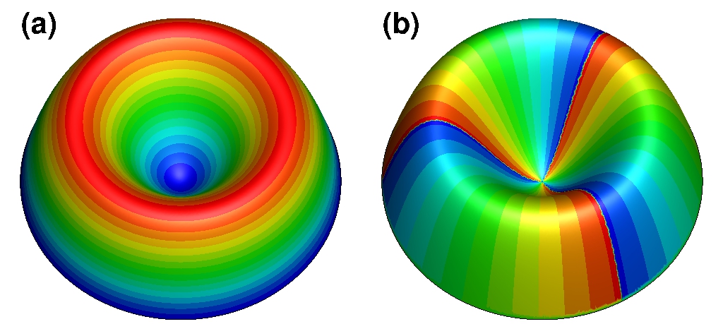
Figure 3: Manufactured solution (42) visualized with a 3D-rendering of the modulus $|u_{ex}|$ color-coded with (a) the modulus itself and (b) the phase of the solution for $m=3$.

It also satisfies an inhomogeneous form of the nonlinear problem (7), i. e.

(43) $$-\frac{1}{2}\nabla^{2}u_{ex}+C_{\text{trap}}u_{ex}+C_{g}|u_{ex}|^{2}u_{ex}-iC_{\Omega}{\bf A}^{t}\cdot\bm{\nabla}u_{ex} = f \text{in}\ {\mathcal{D}},$$

$$u_{ex} = 0 \text{on}\ \partial{\mathcal{D}},$$

and is a critical point of the modified energy functional

(44) $$E(u,f)=\int_{{\mathcal{D}}}\left[\frac{1}{2}|\bm{\nabla}u|^{2}+C_{\text{trap}}\,|u|^{2}+\frac{1}{2}C_{g}|u|^{4}-iC_{\Omega}\,u^{*}{\bf A}^{t}\cdot\bm{\nabla}u-(f^{*}u+fu^{*})\right]\,d{\mathbf{x}}.$$

For this energy functional, the $L^{2}$ gradient is expressed as discussed in §3.1, but with a supplementary term $-2f$ added. Given the form (42) of the manufactured solution and assuming a harmonic trapping potential $C_{\text{trap}}=r^{2}/2$, from (43) we obtain $f(r,\theta)=F(r)\,\exp(im\theta)$, where $F(r)$ is a polynomial of degree 9. From this and relations (44) and (5) we can deduce exact expressions for the energy $E_{ex}:=E(u_{ex})$ and the angular momentum $L_{ex}:=L(u_{ex})=m$.

The numerical tests are based on the manufactured solution (42) corresponding to the following parameter values: $C_{\text{trap}}=r^{2}/2$, $C_{g}=500$, $R=1$, $m=3$, $C_{\Omega}=10$, where, to make the problem more challenging, large values of the nonlinear interaction constant $C_{g}$ and rotation frequency $C_{\Omega}$ are used (cf. Figure 3). The step size $\tau_{n}$ is determined at each iteration by line-minimization (26) for the (PG) method and arc-minimization (29) or (39) for the (RG), (CG) and (RCG) methods.

In order to assess the mesh-independent effect of the Sobolev gradient preconditioning, cf. §5, we perform computations using two grids: Mesh 1 consisting of 24,454 triangles with $h_{min}=0.0118$ and Mesh 2 consisting of 99,329 triangles with $h_{min}=0.0059$, where $h_{min}$ is the smallest grid size. In the present case no mesh refinement was performed during iterations. The initial guess is taken as $u_{0}=0$, whereas iterations are declared converged once the following condition based on the relative energy decrease is satisfied [29, 57]

(45) $$\varepsilon_{E}=|E_{n+1}-E_{n}|/E_{n}<\varepsilon_{st}=10^{-12},\qquad\text{where}\ E_{n}:=E(u_{n}).$$

The performance of the approaches corresponding to the different design choices discussed in §6 is summarized in Table 1 where all computations were performed on Mesh 2. In this and in the following tables the CPU time reflects the computations performed on a Linux workstation with two 3.10GHz Intel Xeon E5-2687w CPUs.

Method	iter	CPU
(RCG)-(PR)-(VtRS)	37	1270
(RCG)-(PR)-(VtDR)	38	1326
(CG)-(PR)	38	1529
(RCG)-(FR)-(VtRS)	54	1852
(RCG)-(FR)-(VtDR)	49	1668
(CG)-(FR)	31	1297
(RG)	180	5274
(PG)	219	3104

Table 1: Test case based on the manufactured solution (42). Performance of the gradient methods corresponding to the different design choices, cf. §6 measured in terms of the number of iterations (iter) and the computational time in seconds (CPU) required for convergence. Note that the total computational time depends both on the number of iterations and the number of evaluations of the energy functional in the line- or arc-minimization procedures.

In the calculations reported in Table 1 for the (CG) and (RCG) methods we did not reset the momentum term $\beta_{n}$ to zero. Firstly, we note that all variants of the (RCG) and (CG) methods outperform the simple gradient methods (PG) and (RG). The reduced CPU time of the (PG) method comes from the fact that it implements a line-minimization strategy (26) based on analytical expressions derived from the particular form of the GP energy (see [57] for details). This is not the case for the arc-minimization used by all Riemannian gradient methods, where an adaptation of Brent’s algorithm is employed. Secondly, we observe that the (RCG) algorithm with the Polak-Ribière (PR) momentum term is least sensitive to the form of the vector transport. On the other hand, the Fletcher-Reeves version of the (RCG) method proves more sensitive to the form of the vector transport and, somewhat surprisingly, the (CG)-(FR) approach (without vector transport) turns out to be the most efficient in terms of the number of iterations (although not in terms of the computational time). The method which converged in the shortest time was the (RCG)-(PR)-(VtRS) approach and it will be used for further tests in the remainder of this section; for brevity, we will refer to it simply as (RCG).

To assess the speed of convergence of the (PG), (RG) and (RCG) approaches, the quantities $\|u_{n}-u_{ex}\|_{2}$ and $|E_{n}-E_{ex}|$ are shown as functions of iterations $n$ for the two spatial discretizations in Figures 4a and 4b. In these figures we observe linear convergence followed by a slower convergence at final iterations. The change of the slope of error curves occurs at the level at which the minimization errors $(u_{n}-u_{ex})$ are comparable to the errors related to the spatial discretization. In other words, in the “optimize-then-discretize” setting adopted here, gradient expressions derived based on the continuous formulation, cf. (15), may no longer accurately represent the sensitivity of the discretized objective function, when the difference between $u_{n}$ and $u_{ex}$ is of the order of the space discretization errors. This is also confirmed by computing the errors $\|u_{n}-u_{ex}\|_{H^{1}}$ at which convergence stagnates. These errors drop by a factor of roughly 4 when the mesh is refined such that $h_{min}$ is reduced by approximately one half (cf. Figure 4a), as expected from the well-known error estimates for the finite-element approximation.

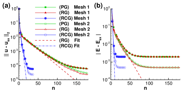
Figure 4: Test case based on the manufactured solution (42). Convergence of the (PG), (RG) and (RCG) methods: (a) $\|(u_{n}-u_{ex})\|_{2}$ and (b) $|E_{n}-E_{ex}|$ are shown as functions of iterations $n$ for different discretizations. Dashed and dash-dotted lines indicate the least-squares fits (46).

In Figures 4a and 4b it is evident that the (RCG) method converges much more rapidly (39 iterations) than the (RG) approach (180 iterations). As expected, the convergence of the (PG) method (202 iterations) is similar to that of the (RG) method. To quantify the convergence rates we use the following ansatz to represent the errors:

(46) $$\|u_{n}-u_{ex}\|_{2}\sim B_{u}\,A_{u}^{n},\qquad|E_{n}-E_{ex}|\sim B_{e}\,A_{e}^{n}.$$

The values of the parameters $A_{u}$ and $A_{e}$, which represent the factors by which the corresponding errors are reduced between two iterations can be obtained from least-squares fits of the data in Figures 4a,b in the linear regime. These results are collected in Table 2 (the corresponding fits are also indicated in Figures 4a,b). First, these results demonstrate that the rate and speed of convergence are grid-independent as expected from the general theory of Sobolev-gradient descent methods [45]. The data in Table 2 can also be interpreted in terms of the classical theory of the conjugate gradient method in the finite-dimensional Euclidean setting [46], which for the minimization of quadratic functions predicts that $A_{u}\approx\sqrt{A_{e}}$. We see that the data from Table 2 satisfies this relationship with the accuracy of a few percent. For the simple gradient and conjugate gradient methods we furthermore have the approximate relationships $A_{u}=(\kappa-1)/(\kappa+1)$ and $A_{u}=(\sqrt{\kappa}-1)/(\sqrt{\kappa}+1)$, respectively, where $\kappa$ is the “effective” condition number characterizing the problem. It is defined in terms of the condition number of the discrete Hessian of the GP energy (1) at the minimum preconditioned by the metric of the Sobolev space $H_{A}({\mathcal{D}})$, cf. (10), in which optimization is performed. Using the data from Table 2 (Mesh 2), we infer that $\kappa\approx 42.37$ for the gradient (RG) and $\kappa\approx 3.2$ for the conjugate gradient (RCG) method, indicating that the convergence acceleration produced in the present problem by the Riemannian conjugate gradient approach actually exceeds what can be expected from the standard theory.

	Mesh 1			Mesh 2
	$A_{e}$	$\sqrt{A_{e}}$	$A_{u}$	$A_{e}$	$\sqrt{A_{e}}$	$A_{u}$
(RG)	0.9167	0.9574	0.9496	0.9268	0.9627	0.9538
(RCG)	0.2909	0.5394	0.5275	0.2924	0.5408	0.5238

Table 2: Parameters characterizing the least-squares fits (46) of the data shown in Figure 4.

Since the exact solution $u_{ex}$ is usually unavailable in physically relevant problems, we now verify that convergence of iterations can be monitored based on quantities which do not involve $u_{ex}$. Indeed, the evolution of $\|u_{n+1}-u_{n}\|_{2}$ and $|E_{n+1}-E_{n}|$ with iterations $n$ shown in Figures 5a and 5b exhibits the same trends as the data shown in Figures 4a and 4b, except for the slowdown observed in the latter case. This demonstrates that either of these two quantities can be used to monitor convergence and, in particular, check the stopping criterion (see also [16, 13, 15, 9, 14]).

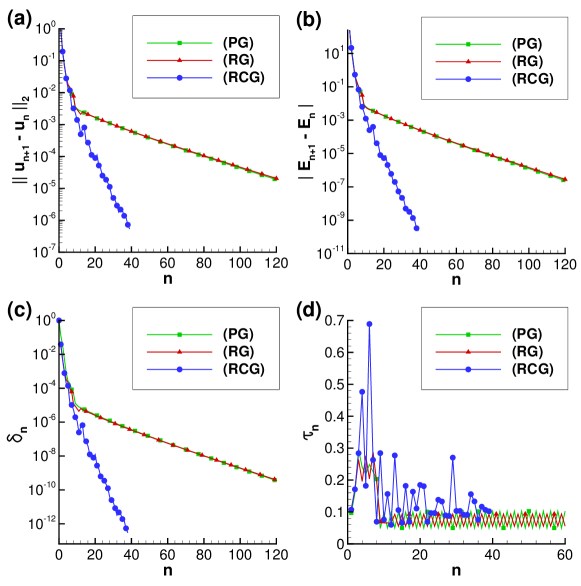
Figure 5: Test case based on the manufactured solution (42). Convergence of the different quantities with iterations $n$: (a) $\|(u_{n+1}-u_{n})\|_{2}$, (b) $|E_{n+1}-E_{n}|$, (c) $\delta_{n}$, cf. (47), drift away from the constraint manifold and (d) $\tau_{n}$, the optimal descent step.

There are two additional aspects of the convergence of the different methods we wish to comment on. In Figure 5c we show the evolution of the “drift” away from the constraint manifold ${\mathcal{M}}$ exhibited by the intermediate approximations $\hat{u}_{n}$ before retraction (27) is applied

(47) $$\delta_{n}=\left|1-{\|\hat{u}_{n}\|^{2}_{2}}\right|,\qquad n=0,1,\dots.$$

This quantity measures how far the intermediate steps diverge from the constraint manifold. We see that, as compared to the (PG) and (RG) methods, in the (RCG) approach the intermediate approximations always remain closer to ${\mathcal{M}}$ . Finally, the step size $\tau_{n}$ determined by the gradient approaches (PG), (RG) and (RCG) via line/arc-minimization, cf. (26), (29) and (39), is shown in Figure 5d. We see that the step sizes generated by the simple gradient methods, (PG) and (RG), tend to oscillate between two values, a behavior indicating that the iterations are trapped in narrow “valleys”. This is a common behavior of the steepest descent method when applied to poorly conditioned problems and is not exhibited by the the (RCG) iterations where on average the steps also tend to be longer. The data in Figure 5a,c,d offers interesting insights about the behavior of iterations in different approaches. It follows from relation (21) that $\|u_{n+1}\|_{2}^{2}-\|u_{n}\|_{2}^{2}=\tau_{n}^{2}\|G_{n}\|_{2}^{2}$ is satisfied for all cases considered here, whereas in Figure 5d it is evident that the corresponding step sizes $\tau_{n}$ are bounded away from zero. We therefore deduce that the drift $\delta_{n}$ is directly linked to the magnitude of the gradient $\|G_{n}\|_{2}$, which is smallest for the approach with the fastest convergence, i. e. the RCG method (cf. Figure 5a). This demonstrates that the small drift away from the constraint manifold ${\mathcal{M}}$ observed in this approach, cf. Figure 5c, is a consequence of its rapid convergence. Performance of the different methods applied to several realistic problems will be discussed in the next section.

8 Computation of Rotating Bose-Einstein Condensates

In this section we compare the performance of the minimization algorithms (PG), (RG) and (RCG) on a number of test cases involving configurations of rotating BEC with vortices. We consider increasingly complex arrangements: a single vortex, Abrikosov vortex lattices with more than one hundred vortices, giant vortices and, finally, condensates in anisotropic trapping potentials. To make these test cases more challenging, we consider large values of the nonlinear interaction constant $C_{g}$ and large angular frequencies $C_{\Omega}$. In some cases, we will provide comparisons between the gradient methods and other state-of-the-art techniques, one of which is the (BE) approach (18)–(19) implemented using the same $P^{2}$ finite-element setting. In addition, in order to offer a comparison with a higher-order method, we will also solve the minimization problem (6) using the library Ipopt which is interfaced with FreeFem++. This approach, which we will refer to as (Ipopt), is based on a combination of an interior point minimization [58], barrier functions [39] and a filter line-search [59]. For problems with equality constraints only (such as the present problem), (Ipopt) reduces to a Newton-like method with an elaborate line-search used to optimally determine the step size. Here we use (Ipopt) to solve the Euler-Lagrange system (7) in the course of which it is provided with the expressions for the $L^{2}$ gradient and the Hessian of the GP energy, reformulated by separating the real and imaginary parts of the solution (see also [57]). Computations with (Ipopt) are based on several calls of the library where, for each call, the residual of the optimality condition (7), on which the termination criterion is based, is progressively decreased.

8.1 Test Case #1: BEC with a Single Central Vortex

We consider the case of a BEC trapped in a harmonic potential and rotating at low angular velocities: $C_{\text{trap}}=r^{2}/2$, $C_{g}=500$, $C_{\Omega}=0.4$. For this case, the Thomas-Fermi (TF) theory [55] offers a good approximation of the atomic density $\rho=|u|^{2}$ of the condensate $\rho\approx\rho_{\hbox{\tiny TF}}=\left((\mu-C^{\text{eff}}_{\text{trap}})/{C_{g}}\right)_{+}$ with the effective trapping potential $C^{\text{eff}}_{\text{trap}}$ given by (12). By imposing $\int_{\cal D}\rho_{\hbox{\tiny TF}}=1$, we can derive analytical expressions for the corresponding approximation of the chemical potential $\mu\in{\mathbb{R}}$ [57]. From the same TF approximation, we can estimate the radius of the condensate as $R_{\hbox{\tiny TF}}=\sqrt{2\mu/(1-C_{\Omega})}$. Consequently, we set up the computational domain ${\mathcal{D}}$ as a disk of radius $R=1.25R_{\hbox{\tiny TF}}=6.56$. The initial guess $u_{0}$ is taken in the form of an off-center vortex placed at $(x_{v}=0.25,y_{v}=0)$, see Figure 6a. We use the ansatz $u_{0}=\sqrt{\rho_{\hbox{\tiny TF}}}\,u_{v}$, where $u_{v}=r/\sqrt{r^{2}+2\xi^{2}}\,e^{i\theta}$ with $(r,\theta)$ representing the polar coordinates centered at $(x_{v},y_{v})$ and $\xi=1/\sqrt{2\mu}$ the non-dimensional healing length, which is a good approximation of the vortex radius in rotating BEC [33]. A similar ansatz will also be used in subsequent sections to set up initial guesses with vortices for the calculation of more complicated BEC configurations. The stopping criterion (45) is used with the value $\varepsilon_{st}=10^{-12}$. In these calculations the grid remains fixed (i. e. no grid adaptation is performed), with 9,578 vertices and 18,825 triangles. In the (BE) method the imaginary time step is chosen as $\delta t=10$, which proved to be optimal for convergence after testing values of $\delta t$ in the range from $0.01$ to $100$. In the (Ipopt) approach, two successive calls to the library were sufficient to converge the solution to the same level of accuracy as with other methods.

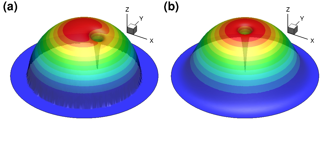
Figure 6: Computation of a rotating BEC with a single central vortex (cf. §8.1). 3D rendering of the atomic density $\rho=|u|^{2}$ for: (a) the initial guess $u_{0}$ and (b) the converged ground state.

For the considered physical parameters the ground state features a vortex centered at the origin. All considered methods, (PG), (RG), (RCG), (BE) and (Ipopt), converged to the same ground state shown in Figure 6b. In order to assess their respective rates of convergence, we compute a reference (“exact”) solution $u_{ex}$ using the same grid and starting the minimization algorithms from the initial guess $u_{0}$ with $(x_{v}=0,y_{v}=0)$. The corresponding energy and angular momentum are $E_{ex}=8.36059$ and $L_{ex}=1$.

The performance of the approaches corresponding to the different design choices discussed in §6 is summarized in Table 3, whereas their convergence monitored in terms the error norm $\|u_{n}-u_{ex}\|_{2}$ is illustrated in Figure 7. As compared with the results analyzed in §7, the difference here is that we now allowed for periodic resets of the momentum term $\beta_{n}$ to zero and it was found by trial-and-error that the fastest convergence in terms of the CPU time was obtained when such resets were performed every 50 iterations. From Table 3 we conclude that the (RCG)-(PR) approach is more robust than the (RCG)-(FR) approach with respect to the choice of the vector transport and the reset frequency. We also note that ignoring the vector transport, which is the case in the (CG) methods, produces a significant increase of the computational time resulting from slow convergence of the arc-minimization procedure. As regards resetting the momentum term to zero, we note that it turns out to be particularly important for the (FR) approaches, concurring with the insights about them already known from the Euclidean setting [46]. In addition to being costly to determine, optimal momentum reset strategies also tend to be strongly problem-dependent. Thus, with this in mind, we conclude that the (RCG)-(PR)-(VtRS) approach again turns out to be the most efficient and is also characterized by the most consistent performance. Therefore, it will be used for further tests in the remainder of this section and we will continue to refer to is as (RCG).

Method	Reset: none		Reset: 50 iter
	iter	CPU	iter	CPU
(RCG)-(PR)-(VtRS)	196	913	190	903
(RCG)-(PR)-(VtDR)	186	954	180	868
(CG)-(PR)	198	1328	184	1271
(RCG)-(FR)-(VtRS)	242	1244	140	637
(RCG)-(FR)-(VtDR)	563	2652	359	1703
(CG)-(FR)	237	1583	150	1077
(RG)	2643	13872
(PG)	3631	8472
(BE)	2796	6838
(Ipopt)	18	99

Table 3: Computation of a rotating BEC with a single central vortex (cf. §8.1). Performance of the gradient methods corresponding to the different design choices, cf. §6, and of the (Ipopt) approach measured in terms of the number of iterations (iter) and the computational time in seconds (CPU) required for convergence.

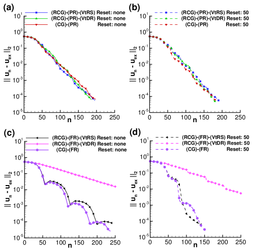
Figure 7: Computation of a rotating BEC with a single central vortex (cf. §8.1). Comparison of different design choices for the (RCG) method in terms of convergence of the error norm $\|u_{n}-u_{ex}\|_{2}$.

The quantities $\|u_{n}-u_{ex}\|_{2}$, $|E_{n}-E_{ex}|$ and $|L_{n}-L_{ex}|$ shown in Figures 8a, 8b and 8c as functions of $n$ indicate that while the (RG) and (BE) methods converge with similar rates, the (RCG) approach converges much faster. The drift $\delta_{n}$ away from the constraint manifold ${\mathcal{M}}$ at intermediate steps $\hat{u}_{n}$, cf. (47), during the first 200 iterations is shown for different methods in Figure 8d. We note that for the (BE) method this quantity is always $\mathcal{O}(1)$ which is due to the fact that the RHS of (18) is based on an unprojected gradient further compounded by a large step size $\delta t$ used. The normalization step is therefore crucial in this approach. On the other hand, $\delta_{n}$ is reduced faster in the (RCG) approach where it also attains lower values than in the (PG) and (RG) methods.

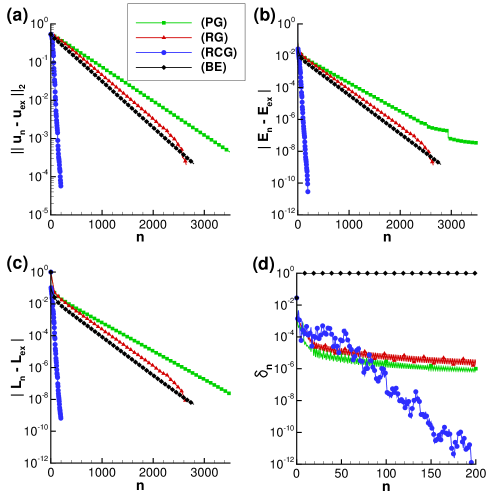
Figure 8: Computation of a rotating BEC with a single central vortex (cf. §8.1). Convergence of the different quantities with iterations $n$: (a) $\|(u_{n}-u_{ex})\|_{2}$, (b) $|E_{n}-E_{ex}|$, (c) $|L_{n}-L_{ex}|$ and (d) $\delta_{n}$, cf. (47), the drift away from the manifold.

Finally, let us note that, even though the (RCG) method outperforms all other first-order methods, the (Ipopt) approach actually converges much faster, cf. Table 3. Only 18 Hessian evaluations are needed during the two calls to Ipopt and the total computational time is smaller by a factor of 10 as compared to the (RCG) methods. However, we stress that this test was performed with a fixed grid and in fact this remarkable performance of the (Ipopt) method will be lost when computing more complicated cases that require mesh adaptivity (see the next section).

8.2 Test Case #2: BEC with a dense Abrikosov vortex lattice

We now move on to consider more challenging test cases corresponding to a harmonic potential ($C_{\text{trap}}=r^{2}/2$), high rotation rate ($C_{\Omega}=0.9$) and large values of the nonlinear interaction constant ($C_{g}=1000$ to $15000$). We note that for the harmonic trapping potential there is a physical limit occurring at the rotation frequency $C_{\Omega}=1$ when the trapping is canceled by the centrifugal force (i. e. $C^{\text{eff}}_{\text{trap}}=0$, see eq. (12)). The next section will consider cases with a modified trapping potential, allowing for higher rotation frequencies.

We start with the case with $C_{g}=1000$ and $C_{\Omega}=0.9$ for which the ground state features over fifty vortices arranged in a regular triangular lattice called the Abrikosov lattice. The difficulty here is to obtain a very regular lattice, in particular for the vortices located near the border of the condensate where the atomic density is low. This explains why the results previously reported for this case exhibit configurations with somewhat different arrangements of the peripheral vortices which nevertheless have very similar energy levels [61, 30, 11]. These differences can be attributed to the use of different initial guesses $u_{0}$. A nearly perfect arrangement of vortices on a triangular/hexagonal lattice is reported in the recent study [60] and will be considered here as a reference result used to validate our methods (the corresponding energy level is $E^{ref}=6.3607$). Details of the computed stationary states depend on the initial guess $u_{0}$, and we used three distinct forms of $u_{0}$: (i) “ansatz d” proposed in [60] to model a central vortex using Gaussian functions, and the Thomas-Fermi approximation described in §8.1 with (ii) one central vortex and (iii) six vortices. The corresponding stationary solutions obtained using the (RCG)-(PR)-(VtRS) method are shown in Figures 9a, 9b and 9c. We can see that the central parts of the vortex lattices are in all cases essentially identical (modulo rotation) and some differences are detected among the peripheral vortices. The values of energy corresponding to these configurations differ by less than $0.01\%$.

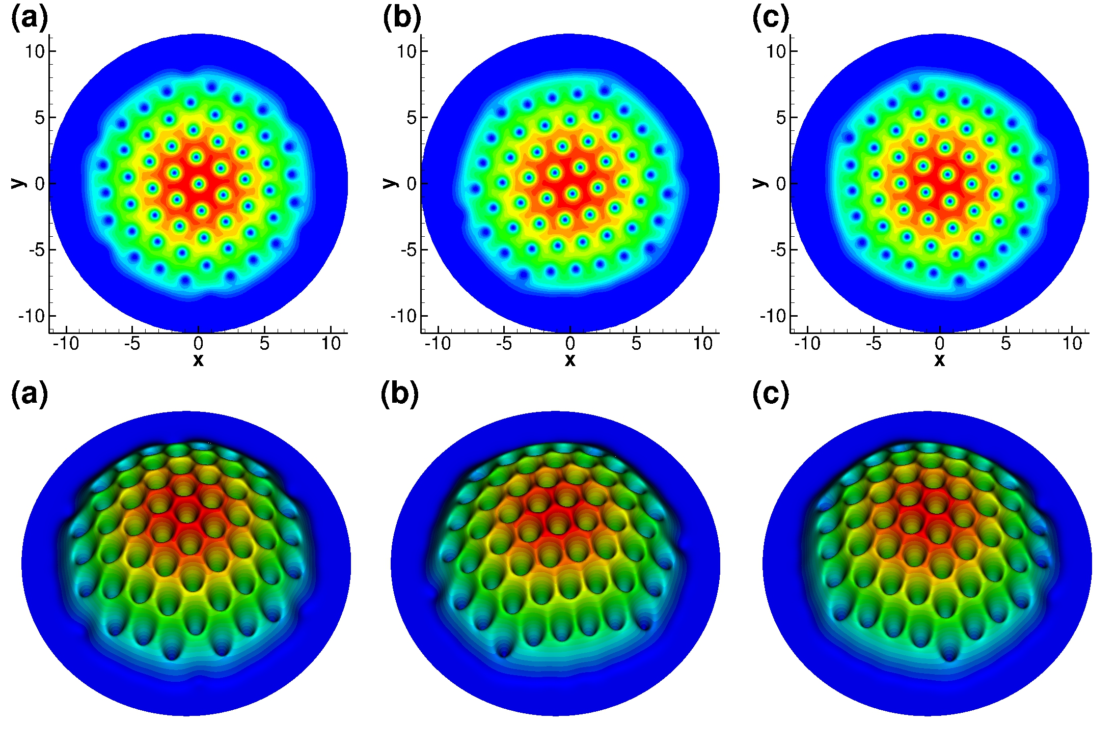
Figure 9: Computation of a rotating BEC with a dense Abrikosov vortex lattice (cf. §8.2). Stationary states obtained using the (RCG)-(PR)-(VtRS) method with mesh adaptivity and different initial conditions $u_{0}$: (a) “ansatz d” suggested in [60], (b) Thomas-Fermi atomic density with one central vortex, (c) Thomas-Fermi atomic density with a ring of six vortices. The figures in the first row show contours of the atomic density (normalized by its maximum value $\rho/\rho_{max}$) and in the second row they show the 3D-rendering of the same contours. The corresponding energies are: (a) $E=6.3615$, (b) $E=6.3621$, (c) $E=6.3620$, to be compared to the reference value $E^{ref}=6.3607$ from [60].

In the following we carry out computations starting from the initial guess (i) and mesh adaptation is now performed during iterations which are declared converged when the termination condition (45) with $\varepsilon_{st}=10^{-9}$ is met. For this challenging test case the performance of a few selected design choices for the (RCG) and (CG) approaches is summarized in Table 4. Since the (FR) methods with and without momentum resets failed to converge to the same minimum as other approaches, we focus here on the (PR) techniques and note the fast convergence of the (RCG)-(PR)-(VtRS) approach which will be used in further tests in this section; for brevity, we will refer to it simply as (RCG). It is interesting to note in Table 4 that the performance of the (Ipopt) method is significantly degraded as compared to the results from §8.1 and is now comparable to that of the (RCG) method. The reason is that Ipopt is linked as an external library to FreeFem++ and therefore we cannot directly use mesh adaptivity in its internal algorithm. As a result, one has to use an external algorithm to couple the computation of the minimizer with the mesh adaptivity procedure employed in the other methods. The computations in the present case required 17 calls to Ipopt, with a total of 354 Hessian evaluations and a large number of internal iterations.

Method	$E$	iter	CPU
(RCG)-(PR)-(VtRS)	6.3615	1339	23192
(RCG)-(PR)-(VtDR)	6.3615	2684	59431
(CG)-(PR)	6.3615	1557	25693
(Ipopt)	6.3621	354	22943

Table 4: Computation of a rotating BEC with a dense Abrikosov vortex using mesh adaptivity and initial condition $u_{0}$ described by the “ansatz d” suggested in [60] (cf. §8.2). Performance of the gradient methods corresponding to the indicated design choices, cf. §6, and of the (Ipopt) approach measured in terms of the number of iterations (iter) and the computational time in seconds (CPU) required for convergence.

Convergence of the iterations carried out with the (RG), (RCG) and (BE) methods is compared in Figures 10a and Figures 10b.

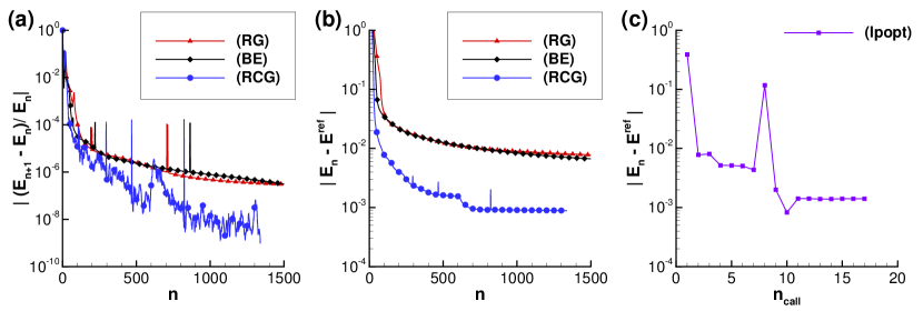
Figure 10: Computation of a rotating BEC with a dense Abrikosov vortex lattice (cf. §8.2). Convergence of the different quantities with iterations $n$: (a) $|(E_{n+1}-E_{n})/E_{n}|$ and (b, c) $|E_{n}-E^{ref}|$. All computations start from the initial guess suggested in [60] (”ansatz d”).

The gradient (RG) and the backward-Euler (BE) methods show a similar, but markedly slower convergence (they were stopped after 5000 iterations) than the (RCG) method. We note that the peaks in the curves shown in Figures 10a and 10b result from reinterpolation of intermediate solutions after grid adaptation [29, 57]. In these figures we see that in all cases convergence slows down at later iterations which is related to the slow rearrangement of vortices near the boundary of the condensate. Another possible reason is that since in [60] a different discretization was used (Fourier spectral approach with periodic boundary conditions), the value of $E^{ref}$ taken from that reference might not exactly correspond to ours. Since convergence is monitored differently for the (Ipopt) method, in Figure 10c we show the decrease of the energy with the number of calls to the library (we add that the energy also tends to exhibit significant oscillations during iterations performed within each such call). While the energy level attained with the (Ipopt) method is a little higher than obtained with the (RCG) and (CG) methods, the corresponding minimizer is similar to that shown in Figure 9c.

8.3 Test Case #3: BEC with a large number of vortices

In this section, we use the (RCG)-(PR)-(VtRS) method to compute fast rotating BEC ($C_{\Omega}=0.9$) corresponding to large values of the nonlinear interaction constant with $C_{g}$ varying from 1,000 to 15,000. For these difficult cases, a more physically relevant assessment of the convergence of iterations is provided by the alignment of vortices on parallel lines inside the vortex lattice. Since isocontours of atomic density do not always coincide with these lines, we developed a post-processing approach to identify the centers of vortices by detecting local minima of the function $\rho_{\hbox{\tiny TF}}-\rho$. This post-processing is similar to that used for experimental data [27] or 3D numerical simulations [28] and also allows to build the Delaunay triangulation of the lattice and compute the radius of each vortex. The resulting stationary states are presented in this way in Figure 11. We notice an arrangement of vortices on a nearly perfect lattice for $C_{g}=1,000$ and $5,000$, and a less regular arrangement for $C_{g}=10,000$ and $15,000$ with the presence of some defects in the lattice. This effect could be related to physical theories addressing the non-uniformity of the inter-vortex spacing in dense Abrikosov lattices [27, 53].

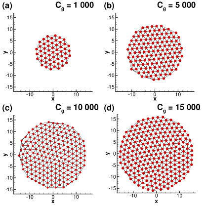
Figure 11: Computation of a fast rotating BEC ($C_{\Omega}=0.9$) in a harmonic trapping potential (cf. §8.2). The Abrikosov vortex lattice is represented using the Delaunay triangulation built from the detected vortex centers. Configurations obtained for large values of the nonlinear interaction constant: $C_{g}=1000$ (55 vortices), $C_{g}=5000$ (134 vortices), $C_{g}=10000$ (193 vortices) and $C_{g}=15000$ (237 vortices).

8.4 Test Case #4: BEC with giant vortex

To overcome the limit $C_{\Omega}=1$ imposed by the harmonic trapping potential, a modified “harmonic-plus-Gaussian” potential was tested in experiments [20]. In [5, 28] this new experimental set-up was modeled as

(48) $$C_{\text{trap}}(x,{y})=(1-\alpha)r^{2}+\frac{1}{4}kr^{4},$$

with the possibility to switch from a “quartic-plus-quadratic” potential ($\alpha<1$), which corresponds to experiments, to a “quartic-minus-quadratic” potential ($\alpha>1$), which is experimentally feasible but was never tested. Adapting the analysis from [5] to our 2D case, we obtain three possible regimes depending on the type of potential:
$\bullet$ Regime 1: “quartic-plus-quadratic” (or weak attractive) potential obtained for $\alpha<1$ and $\mu>0$ (see the Thomas-Fermi approximation in §8.1).
$\bullet$ Regime 2: weak “quartic-minus-quadratic” (or weak repulsive) potential obtained when $\alpha>1$ and $\mu>0$; this regime appears when $|1-\alpha|<\left(k\sqrt{3C_{g}/\pi}\right)/2$.
$\bullet$ Regime 3: strong “quartic-minus-quadratic” (or strong repulsive) potential obtained when $\alpha>1$ and $\mu<0$; this regime appears when $|1-\alpha|>\left(k\sqrt{3C_{g}/\pi}\right)/2$.

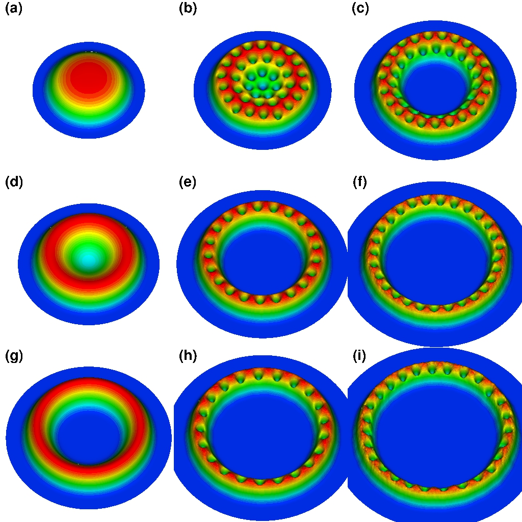
Figure 12: Computation of a rotating BEC with giant vortices (cf. §8.4). 3D-rendering of the atomic density (normalized by its maximum value $\rho/\rho_{max}$) obtained in Regime 1 (a, b, c), Regime 2 (d, e, f) and Regime 3 (g, h, i) for different rotations $C_{\Omega}=0$ (first column), $C_{\Omega}=3$ (second column) and $C_{\Omega}=4$ (third column).

All computations are performed with the (RGC)-(PR)-(VrRS) method and the obtained stationary states are presented in Figure 12. The parameters for these simulations are: $C_{g}=1000$, $k=1$ and $\alpha=1/2$ (Regime 1), $\alpha=11/2$ (Regime 2), $\alpha=9$ (Regime 3). In the first column of Figure 12 we notice that the atomic density distribution in the condensate without rotation ($C_{\Omega}=0$) changes from the classical parabolic profile in Regime 1 to a Mexican-hat type profile in Regime 2 and, finally, to a profile with a central hole in Regime 3. It is then expected that, when rotation is applied, in Regimes 2 and 3 the condensate will develop a central hole (or giant vortex) at lower rotations frequencies than in Regime 1. This prediction is indeed supported by the results in Figure 12 (second and third column). When rotation is increased, the condensate configuration evolves from a classical (Abrikosov) vortex lattice to a vortex lattice with a central depletion and, finally, to a giant vortex surrounded by a ring of individual vortices. The giant vortex is indeed obtained for lowest rotation frequencies in Regimes 2 and 3. The existence of a giant vortex was predicted theoretically (e. g. [33]) and was already observed in 2D [40] and 3D computations [5, 28].

8.5 Test Case #5: Strongly Anisotropic BEC with Vortices

To demonstrate the efficiency of the (RGC)-(PR)-(VrRS) method for the case without any symmetry, in this section we consider a rotating BEC trapped in a strongly anisotropic (asymmetrical) potential of the form suggested in [47]

(49) $$C_{\text{trap}}(x,{y})=\frac{1}{2}\left[(1+\eta^{2})x^{2}+(1-\eta)y^{2}\right],\quad\eta=2(1-C_{\Omega})\epsilon,$$

where $\epsilon<1$ characterizes the anisotropy of the trap for very high rotation frequencies $C_{\Omega}\approx 1$. The theoretical analysis presented in [47] shows that, when the condensate contains a large number of vortices, the deviation of the vortex lattice from a triangular arrangement is small. This finding is supported by our computational results shown in Figure 13 for three values of the anisotropy parameter $\epsilon$. This example illustrates the flexibility of the finite-element discretization, cf. §5, in handling highly deformed computational domains ${\mathcal{D}}$.

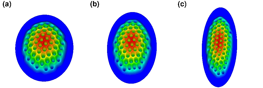
Figure 13: Computation of a rotating BEC in a strongly anisotropic trapping potential (cf. §8.5). 3D-rendering of the atomic density (normalized by its maximum value $\rho/\rho_{max}$) obtained for $\epsilon=0.15$ (a), $\epsilon=0.35$ (b), $\epsilon=0.65$ (c).

9 Conclusions

The difficulty of direct minimization of the Gross-Pitaevskii energy functional with rotation comes from the unit-norm constraint (2). The novel idea proposed here is to transform this problem to an unconstrained Riemannian optimization problem defined on a spherical manifold and then develop a Riemannian conjugate gradient (RCG) method based on classical approaches. The key ingredients of this new method are the following: (i) the gradient direction is derived using the theory of Sobolev gradients and relies on a physically-inspired definition of the inner product which accounts for rotation [30], thereby offering a good preconditioning for the problem; (ii) the gradient is projected on the subspace tangent to the spherical manifold before being used in simple gradient or conjugate gradient methods, which ensures the iterates stay close to manifold ${\mathcal{M}}$; (iii) the conjugate descent direction is computed using classical approaches (i. e. the Polak-Ribière or Fletcher-Reeves variant of the nonlinear conjugate gradient method) and the Riemannian vector transport is used to bring the gradient and descent directions determined at the previous iteration to the current tangent subspace ${\cal T}_{u_{n}}{\cal M}$; (iv) the optimal descent step is computed by solving an arc-minimization problem (in which samples are constrained to lie on the manifold), instead of the classical line-minimization; (v) finally, the updated solution is “retracted” back to the spherical manifold. In our study we carefully analyzed the effect of the key design choices, namely, the form of the momentum term and of the vector transport, on the performance of the Riemannian conjugate gradients approach. Based on tests involving several different problems, we conclude that the (RGC)-(PR)-(VrRS) approach, combining the Polak-Ribière form of the momentum term with the vector transport based on the Riemannian submanifold structure, exhibited the most robust and efficient performance. The (RCG)-(PR) methods in general also showed a systematic improvement over the (CG) approaches without vector transport.

As demonstrated by our tests performed in the finite-element setting, several features make the (RCG) method very appealing for practical computations: (i) since the “optimize-then-discretize” paradigm is used, the preconditioning is mesh-independent; (ii) the Riemannian retraction and transport operators are simple to implement; (iii) for the arc-minimization problem a classical approach such as Brent’s method can be easily adapted; (iv) there are no tuning parameters or trust-region tests involved. In addition, general mesh refinement or mesh adaptivity strategies are compatible with the RCG method without any modifications. Our extensive numerical experiments showed a significant improvement of the convergence rate of the RCG method over the simple gradient and imaginary-time methods. For more involved problems requiring mesh adaptation the (RCG) approach exhibited performance comparable to the (Ipopt) method which for equality-constrained problems implements a Newton-type technique. The reason is that there is no straightforward way to incorporate mesh adaptation in the (Ipopt) approach, something that can be done rather easily in the (RCG) method. We stress that the use of mesh adaptation is essential for efficient computational solution of problems of the type discussed in §§8.2–8.5 and, to the best of our knowledge, implementation of mesh adaptation in Ipopt-type, or more generally, in Newton-type methods, remains an open problem. We also emphasize that the (RCG) approach has far fewer parameters than the (Ipopt) method which greatly simplifies its performance optimization. Finally, as a challenging test, the (RCG) method was used to compute vortex configurations in rotating BEC with high values of the nonlinear interaction constants and very high rotation rates as well as in configurations with strongly anisotropic trapping potentials.

Lastly, we reiterate that the approach presented in this study does not exploit all opportunities inherent in the Riemannian formulation. In particular, it remains an open question whether the use of a well-adapted Riemannian metric defined on the constraint manifold could further improve the performance of the approach. In addition, one can also consider the Riemannian formulations of Newton’s method and of different variants of the quasi-Newton method. Work is already on-going on some of these problems and results will be reported in the near future.

The authors are grateful to the anonymous referees for providing constructive feedback on this manuscript.

References

- [1] P.-A. Absil, R. Mahony, and R. Sepulchre, Optimization Algorithms on Matrix Manifolds, Princeton University Press, 2008.
- [2] R. A. Adams and J. F. Fournier, Sobolev Spaces, Elsevier, 2005.
- [3] A. Aftalion, Vortices in Bose-Einstein Condensates, Birkhauser, 2006.
- [4] A. Aftalion and I. Danaila, Three-dimensional vortex configurations in a rotating Bose-Einstein condensate, Physical Review A, 68 (2003), pp. 023603(1–6).
- [5] A. Aftalion and I. Danaila, Giant vortices in combined harmonic and quartic traps, Physical Review A, 69 (2004), pp. 033608(1–6).
- [6] A. Aftalion and Q. Du, Vortices in a rotating Bose-Einstein condensate: critical angular velocities and energy diagrams in the Thomas-Fermi regime, Phys. Rev. A, 64 (2001), p. 063603.
- [7] F. Alouges, A new algorithm for computing liquid crystal stable configurations: The harmonic mapping case, SIAM Journal on Numerical Analysis, 34 (1997), pp. 1708–1726.
- [8] F. Alouges and C. Audouze, Gradient flows, and application to the Hartree-Fock functional, Numer. Meth. for PDE, 25 (2009), pp. 380–400.
- [9] X. Antoine, C. Besse, and W. Bao, Computational methods for the dynamics of the nonlinear Schrödinger/Gross-Pitaevskii equations, Comput. Phys. Comm., 184 (2013), pp. 2621–2633.
- [10] X. Antoine, C. Besse, R. Duboscq, and V. Rispoli, Acceleration of the imaginary time method for spectrally computing the stationary states of Gross-Pitaevskii equations, hal-01356227, (2016).
- [11] X. Antoine and R. Duboscq, Robust and efficient preconditioned Krylov spectral solvers for computing the ground states of fast rotating and strongly interacting Bose-Einstein condensates, J. Comput. Physics, 258 (2014), pp. 509–523.
- [12] X. Antoine, A. Levitt, and Q. Tang, Efficient spectral computation of the stationary states of rotating Bose-Einstein condensates by the preconditioned nonlinear conjugate gradient method, arxiv:1611.02045, (2016).
- [13] W. Bao, Ground states and dynamics of rotating Bose-Einstein condensates, Modeling and Simulation in Science, Engineering and Technology, Birkhauser, 2006, pp. 215–255.
- [14] W. Bao, Mathematical models and numerical methods for Bose-Einstein condensation, Proc. of the International Congress of Mathematicians (Seoul 2014), IV (2014), pp. 971–996.
- [15] W. Bao and Y. Cai, Mathematical theory and numerical methods for Bose-Einstein condensation, Kinetic and related models, 6 (2013), pp. 1–135.
- [16] W. Bao and Q. Du, Computing the ground state solution of Bose-Einstein condensates by a normalized gradient flow, Siam J. Sci. Comput., 25 (2004), p. 1674.
- [17] W. Bao and J. Shen, A generalized Laguerre-Hermite pseudospectral method for computing symmetric and central vortex states in Bose-Einstein condensates, J. Comput. Physics, 227 (2008), pp. 9778–9793.
- [18] W. Bao and W. Tang, Ground-state solution of Bose-Einstein condensate by directly minimizing the energy functional, J. Comp. Physics.
- [19] N. Boumal, B. Mishra, P.-A. Absil, and R. Sepulchre, Manopt, a Matlab toolbox for optimization on manifolds, J. of Machine Learning Research, 15 (2014), pp. 1455–1459.
- [20] V. Bretin, S. Stock, Y. Seurin, and J. Dalibard, Fast rotation of a Bose-Einstein condensate, Phys. Rev. Lett., 92 (2004), p. 050403.
- [21] M. Caliari and S. Rainer, GSGPEs: A Matlab code for computing the ground state of systems of Gross-Pitaevskii equations, Comput. Phys. Comm., 184 (2013), pp. 812 – 823.
- [22] R. Caplan, NLSEmagic: Nonlinear Schrödinger equation multi-dimensional Matlab-based GPU-accelerated integrators using compact high-order schemes, Comput. Phys. Comm., 184 (2013), pp. 1250–1271.
- [23] M. Castro-Diaz, F. Hecht, and B. Mohammadi, Anisotropic grid adaptation for inviscid and viscous flows simulations, Int. J. Comput. Fluid Dynamics, 25 (2000), pp. 475–491.
- [24] S.-L. Chang, C.-S. Chien, and B.-W. Jeng, Computing wave functions of nonlinear Schrödinger equations: A time-independent approach, J. Comput. Physics, 226 (2007), pp. 104 – 130.
- [25] E. Charalampidis, P. Kevrekidis, and P. Farrell, Computing stationary solutions of the two-dimensional gross-pitaevskii equation with deflated continuation, Communications in Nonlinear Science and Numerical Simulation, 54 (2018), pp. 482 – 499.
- [26] P. G. Ciarlet, The finite element method for elliptic problems, Studies in Mathematics and its Applications, North-Holland, 1978.
- [27] I. Coddington, P. C. Haljan, P. Engels, V. Schweikhard, S. Tung, and E. A. Cornell, Experimental studies of equilibrium vortex properties in a Bose-condensed gas, Phys. Rev. A, 70 (2004), p. 063607.
- [28] I. Danaila, Three-dimensional vortex structure of a fast rotating Bose-Einstein condensate with harmonic-plus-quartic confinement, Phys. Review A, 72 (2005), pp. 013605(1–6).
- [29] I. Danaila and F. Hecht, A finite element method with mesh adaptivity for computing vortex states in fast-rotating Bose-Einstein condensates, J. Comput. Physics, 229 (2010), pp. 6946–6960.
- [30] I. Danaila and P. Kazemi, A new Sobolev gradient method for direct minimization of the Gross–Pitaevskii energy with rotation, SIAM J. Sci. Computing, 32 (2010), pp. 2447–2467.
- [31] C. M. Dion and E. Cancès, Ground state of the time-independent Gross-Pitaevskii equation, Comput. Phys. Comm., 177 (2007), pp. 787–798.
- [32] I. Faragò and J. Karàtson, Numerical solution of nonlinear elliptic problems via preconditioning operators: Theory and applications, NOVA Science Publishers, New York, 2002.
- [33] A. L. Fetter, Rotating vortex lattice in a Bose-Einstein condensate trapped in combined quadratic and quartic radial potentials, Phys. Rev. A, 64 (2001), p. 063608.
- [34] J. J. García-Ripoll and V. M. Pérez-García, Optimizing Schrödinger functionals using Sobolev gradients: application to quantum mechanics and nonlinear optics, SIAM J. Sci. Comput., 23 (2001), pp. 1315–1333.
- [35] M. D. Gunzburger, Perspectives in Flow Control and Optimization, SIAM, 2003.
- [36] F. Hecht, New developments in Freefem++, Journal of Numerical Mathematics, 20 (2012), pp. 251–266.
- [37] F. Hecht, O. Pironneau, A. L. Hyaric, and K. Ohtsuke, FreeFem++ (manual), www.freefem.org, 2007.
- [38] U. Hohenester, OCTBEC a Matlab toolbox for optimal quantum control of Bose-Einstein condensates, Comput. Phys. Comm., 185 (2014), pp. 194–216.
- [39] A. W. J. Nocedal and R. A. Waltz, Adaptive barrier strategies for nonlinear interior methods, SIAM Journal on Optimization, 19(4) (2008), pp. 1674–1693.
- [40] K. Kasamatsu, M. Tsubota, and M. Ueda, Giant hole and circular superflow in a fast rotating Bose-Einstein condensate, Phys. Rev. A, 66 (2002), p. 053606.
- [41] P. Kazemi and M. Eckart, Minimizing the Gross-Pitaevskii energy functional with the Sobolev gradient– analytical and numerical results, Int. J. of Comput. Methods, 7 (2009).
- [42] E. H. Lieb and R. Seiringer, Derivation of the Gross-Pitaevskii equation for rotating Bose gases, Comm. in Math. Physics, 264 (2006), pp. 505–537.
- [43] D. Luenberger, Optimization by Vector Space Methods, John Wiley and Sons, 1969.
- [44] B. Merlet and T. N. Nguyen, Convergence to equilibrium for discretizations of gradient-like flows on Riemannian manifolds, Differential Integral Equations, 26 (2013), pp. 571–602.
- [45] J. W. Neuberger, Sobolev Gradients and Differential Equations, Lecture notes in mathematics, 1670, Springer, Berlin/Heidelberg, 1997 (2nd Edition 2010).
- [46] J. Nocedal and S. Wright, Numerical Optimization, Springer, 2002.
- [47] M. Ö. Oktel, Vortex lattice of a Bose-Einstein condensate in a rotating anisotropic trap, Phys. Rev. A, 69 (2004), p. 023618.
- [48] M. Pierre, Newton and conjugate gradient for harmonic maps from the disc into the sphere, ESAIM Control Optim. Calc. Var., 10 (2004), pp. 142–167.
- [49] L. P. Pitaevskii and S. Stringari, Bose-Einstein condensation, Clarendon Press, Oxford, 2003.
- [50] W. H. Press, B. P. Flanner, S. A. Teukolsky, and W. T. Vetterling, Numerical Recipes: the Art of Scientific Computations, Cambridge University Press, 1986.
- [51] W. Ring and B. Wirth, Optimization methods on Riemannian manifolds and their application to shape space, SIAM Journal on Optimization, 22 (2012), pp. 596–627.
- [52] P. J. Roache, Verification and Validation in Computational Science and Engineering, Hermosa Publishers, 1998.
- [53] D. E. Sheehy and L. Radzihovsky, Vortices in spatially inhomogeneous superfluids, Phys. Rev. A, 70 (2004), p. 063620.
- [54] S. T. Smith, Optimization techniques on Riemannian manifolds, Fields Institute Communications, 3 (1994).
- [55] S. Stringari, Phase diagram of quantized vortices in a trapped Bose-Einstein condensed gas, Phys. Rev. Lett., 82 (1999), p. 4371.
- [56] M. Tsubota, Quantized vortices in superfluid helium and Bose-Einstein condensates, Journal of Physics: Conference Series, 31 (2006), p. 88.
- [57] G. Vergez, I. Danaila, S. Auliac, and F. Hecht, A finite-element toolbox for the stationary Gross-Pitaevskii equation with rotation, Comput. Phys. Comm., 209 (2016), pp. 144–162.
- [58] A. Wächter, An interior point algorithm for large-scale nonlinear optimization with applications in process engineering, PhD thesis, Carnegie Mellon University, Pittsburgh, PA, USA, (January 2002).
- [59] A. Wächter and L. T. Biegler, On the implementation of an interior-point filter line-search algorithm for large-scale nonlinear programming, Mathematical Programming, 106 (2006), pp. 25–57.
- [60] X. Wu, Z. Wen, and W. Bao, A regularized Newton method for computing ground states of Bose-Einstein condensates, arXiv: 1504.02891, (2015).
- [61] R. Zeng and Y. Zhang, Efficiently computing vortex lattices in rapid rotating Bose-Einstein condensates, Comput. Phys. Comm., 180 (2009), pp. 854–860.