Assesment of Smarandache Curves in The Null Cone $\mathbf{Q}^{2}$

Mihriban Kulahci Department of Mathematics, Firat University, 23119 ELAZIĞ/TÜRKİYE mihribankulahci@gmail.com  and  Fatma Almaz fb_fat_almaz@hotmail.com
(Date: 2017)
Abstract.

In this paper, we give Smarandache curves according to the asymptotic orthonormal frame in null cone $\mathbf{Q}^{2}$. By using cone frame formulas, we present some characterizations of Smarandache curves and calculate cone frenet invariants of these curves. Also, we illustrate these curves with an example.

Key words and phrases:
Smarandache curve, asymptotic orthonormal frame, null cone, cone frame formulas.
2000 Mathematics Subject Classification:
Primary 53A40; Secondary 53A35
This paper is in final form and no version of it will be submitted for publication elsewhere.

1. Introduction

Human being were bewitched by curves and curved shapes long before they took into account them as mathematical objects. But the greatest effect in the research of curves was, of course, the discovery of the calculus. Geometry before calculus includes only the simplest curves.

In classical curve theory, the geometry of a curve in three-dimensions is actually characterized by Frenet vectors.

Smarandache geometry is a geometry which has at least one Smarandachely denied axiom [4]. An axiom is said to be Smarandachely denied, if it behaves in at least two different ways within the same space. Smarandache curve is defined as a regular curve whose position vector is composed by Frenet frame vectors of another regular curve. Smarandache curves in various ambient spaces have been classfied in [1]-[14], [19], [21]-[32].

In this study, we define special Smarandache curves such as $x\alpha,xy,\alpha y$ and $x\alpha y$ Smarandache curves according to asymptotic orthonormal frame in the null cone $\mathbf{Q}^{2}$ and we examine the curvature and the asymptotic orthonormal frame’s vectors of Smarandache curves. We also give an example related to these curves.

2. Preliminaries

Some basics of the curves in the null cone are provided from, [15]-[18].

Let $E_{1}^{3}$ be the $3-$dimensional pseudo-Euclidean space with the

$$\widetilde{g}(X,Y)=\langle X,Y\rangle=x_{1}y_{1}+x_{2}y_{2}-x_{3}y_{3}$$

for all $X=(x_{1},x_{2},x_{3}),$ $Y=(y_{1},y_{2},y_{3})\in E_{1}^{3}$. $E_{1}^{3}$ is a flat pseudo-Riemannian manifold of signature $(2,1)$.

Let $M$ be a submanifold of $E_{1}^{3}$. If the pseudo-Riemannian metric $\widetilde{g}$ of $E_{1}^{3}$ induces a pseudo-Riemannian metric $g$(respectively, a Riemannian metric, a degenerate quadratic form) on $M$, then $M$ is called a timelike( respectively, spacelike, degenerate) submanifold of $E_{1}^{3}.$ Let $c$ be a fixed point in $E_{1}^{3}.$ The pseudo-Riemannian lightlike cone(quadric cone ) is defined by

$$\mathbf{Q}_{1}^{2}(c)=\left\{x\in E_{1}^{3}:g(x-c,x-c)=0\right\},$$

where the point $c$ is called the center of $\mathbf{Q}_{1}^{2}(c)$. When $c=0$, we simply denote $\mathbf{Q}_{1}^{2}(0)$ by $\mathbf{Q}^{2}$ be and call it the null cone.

Let $E_{1}^{3}$ be $3$-dimensional Minkowski space and $\mathbf{Q}^{2}$ the lightlike cone in $E_{1}^{3}.$ A vector Vβ‰ 0𝑉0V\neq 0 Β Β in $E_{1}^{3}$ is called spacelike, timelike or lightlike, if $\langle V,V\rangle>0$, $\langle V,V\rangle<0$ or $\langle V,V\rangle=0,$ respectively. The norm of a vector $x\in E_{1}^{3}$ is given by $\left\|x\right\|=\sqrt{\left\langle x,x\right\rangle},$ [20].

We assume that curve $x:I\rightarrow\mathbf{Q}^{2}\subset E_{1}^{3}$ is a regular curve in $\mathbf{Q}^{2}$ for $t\in I.$ In the following, we always assume that the curve is regular.

A frame field $\left\{x,\alpha,y\right\}$ on $E_{1}^{3}$ is called an asymptotic orthonormal frame field, if

$$\langle x,x\rangle=\langle y,y\rangle=\langle x,\alpha\rangle=\langle y,\alpha\rangle=0,\text{ }\langle x,y\rangle=\langle\alpha,\alpha\rangle=1.$$

Using Β x′​(s)=α​(s)superscriptπ‘₯′𝑠𝛼𝑠x^{\prime}(s)=\alpha(s) we know that $\left\{x(s),\alpha(s),y(s)\right\}$ from an asymptotic orthonormal frame along the curve $x(s)$ and the cone frenet formulas of $x(s)$ are given by

$\displaystyle x^{\prime}(s)$ $\displaystyle=\alpha(s)$
(2.1) $\displaystyle\alpha^{\prime}(s)$ =κ​(s)​x​(s)βˆ’y​(s)absentπœ…π‘ π‘₯𝑠𝑦𝑠\displaystyle=\kappa(s)x(s)-y(s)
$\displaystyle y^{\prime}(s)$ =βˆ’ΞΊβ€‹(s)​α​(s)absentπœ…π‘ π›Όπ‘ \displaystyle=-\kappa(s)\alpha(s)

where the function κ​(s)πœ…π‘ \kappa(s) is called cone curvature function of the curve $x(s)$, [17].

Let $x:I\rightarrow\mathbf{Q}^{2}\subset E_{1}^{3}$ be a spacelike curve in $\mathbf{Q}^{2}$ with an arc length parameter $s.$ Then $x=x(s)=(x_{1},x_{2},x_{3})$ can be written as

(2.2) $$x(s)=\frac{f_{s}^{-1}}{2}(f^{2}-1,2f,f^{2}+1)$$

for some non constant function $f(s)$ and $f_{s}=f^{\prime}$, [18].

3. Smarandache Curves in The Null Cone $\mathbf{Q}^{2}$

In this section, we define the Smarandache curves according to the asymptotic orthonormal frame in $\mathbf{Q}^{2}$. Also, we obtain the asymptotic orthonormal frame and cone curvature function of the Smarandache partners lying on $\mathbf{Q}^{2}$ using cone frenet formulas.

Smarandache curve Ξ³=γ​(sβˆ—β€‹(s))𝛾𝛾superscriptπ‘ βˆ—π‘ \gamma=\gamma(s^{\ast}(s)) of the curve $x$ is a regular unit speed curve lying fully on $\mathbf{Q}^{2}$. Let $\left\{x,\alpha,y\right\}$ and $\left\{\gamma,\alpha_{\gamma},y_{\gamma}\right\}$ be the moving asymptotic orthonormal frames of $x$ and $\gamma,$ respectively.

Definition 1.

Let $x$ be unit speed spacelike curve lying on $\mathbf{Q}^{2}$ with the moving asymptotic orthonormal frame $\left\{x,\alpha,y\right\}.$ Then, $x\alpha-$smarandache curve of $x$ is defined by

(3.1) Ξ³x​α​(sβˆ—)=cb​x​(s)+α​(s),subscript𝛾π‘₯𝛼superscriptπ‘ βˆ—π‘π‘π‘₯𝑠𝛼𝑠\gamma_{x\alpha}(s^{\ast})=\frac{c}{b}x(s)+\alpha(s),

where $c,b\in\mathbb{R}_{0}^{+}.$

Theorem 1.

Let $x$ be unit speed spacelike curve in $\mathbf{Q}^{2}$ with the moving asymptotic orthonormal frame $\left\{x,\alpha,y\right\}$ and cone curvature κ​(s)πœ…π‘ \kappa(s) and let $\gamma_{x\alpha}$ be $x\alpha-$smarandache curve with asymptotic orthonormal frame $\left\{\gamma_{x\alpha},\alpha_{x\alpha},y_{x\alpha}\right\}.$ Then the following relations hold:

i) The asymptotic orthonormal frame $\left\{\gamma_{x\alpha},\alpha_{x\alpha},y_{x\alpha}\right\}$ of the $x\alpha$-smarandache curve $\gamma_{x\alpha}$ is given as

(3.2) $$\begin{bmatrix}\gamma_{x\alpha}\\ \alpha_{x\alpha}\\ y_{x\alpha}\end{bmatrix}=\begin{bmatrix}\frac{c}{b}&1&0\\ \psi&\frac{b}{c}\kappa\psi&-\frac{b}{c}\psi\\ \varrho_{1}&\varrho_{2}&\varrho_{3}\end{bmatrix}\begin{bmatrix}x\\ \alpha\\ y\end{bmatrix}$$

where

(3.3) $\displaystyle\psi$ $\displaystyle=\frac{c}{\sqrt{c^{2}-2\kappa b^{2}}},$
$\displaystyle\Upsilon_{1}$ $\displaystyle=\frac{b}{c}(\frac{b}{c}\kappa^{\prime}+\kappa)\psi\psi^{\prime}+\frac{b^{2}}{c^{2}}\kappa\left(\psi^{\prime}\right)^{2},$
(3.4) $\displaystyle\Upsilon_{2}$ $\displaystyle=\frac{b}{c}\psi(\psi^{\prime}+2\frac{b}{c}\kappa\psi),$
$\displaystyle\Upsilon_{3}$ $\displaystyle=-\frac{b}{c}\psi(\frac{b}{c}\psi^{\prime}+\psi)$

and

$\displaystyle\varrho_{1}$ =βˆ’(Ξ₯1+c2​b​(2​Ξ₯1​Ξ₯3+Ξ₯22))=βˆ’Ξ₯1+cb​κγx​α​(sβˆ—),absentsubscriptΞ₯1𝑐2𝑏2subscriptΞ₯1subscriptΞ₯3superscriptsubscriptΞ₯22subscriptΞ₯1𝑐𝑏subscriptπœ…subscript𝛾π‘₯𝛼superscriptπ‘ βˆ—\displaystyle=-(\Upsilon_{1}+\frac{c}{2b}\left(2\Upsilon_{1}\Upsilon_{3}+\Upsilon_{2}^{2}\right))=-\Upsilon_{1}+\frac{c}{b}\kappa_{\gamma_{x\alpha}}(s^{\ast}),
(3.5) $\displaystyle\varrho_{2}$ =βˆ’(Ξ₯2+12​(2​Ξ₯1​Ξ₯3+Ξ₯22))=βˆ’Ξ₯2+ΞΊΞ³x​α​(sβˆ—),absentsubscriptΞ₯2122subscriptΞ₯1subscriptΞ₯3superscriptsubscriptΞ₯22subscriptΞ₯2subscriptπœ…subscript𝛾π‘₯𝛼superscriptπ‘ βˆ—\displaystyle=-(\Upsilon_{2}+\frac{1}{2}\left(2\Upsilon_{1}\Upsilon_{3}+\Upsilon_{2}^{2}\right))=-\Upsilon_{2}+\kappa_{\gamma_{x\alpha}}(s^{\ast}),
$\displaystyle\varrho_{3}$ $\displaystyle=-\Upsilon_{3}.$

ii) The cone curvature ΞΊΞ³x​α​(sβˆ—)subscriptπœ…subscript𝛾π‘₯𝛼superscriptπ‘ βˆ—\kappa_{\gamma_{x\alpha}}(s^{\ast}) of the curve $\gamma_{x\alpha}$ is given by

(3.6) ΞΊΞ³x​α​(sβˆ—)=βˆ’12​(2​Ξ₯1​Ξ₯3+Ξ₯22).subscriptπœ…subscript𝛾π‘₯𝛼superscriptπ‘ βˆ—122subscriptΞ₯1subscriptΞ₯3superscriptsubscriptΞ₯22\kappa_{\gamma_{x\alpha}}(s^{\ast})=-\frac{1}{2}\left(2\Upsilon_{1}\Upsilon_{3}+\Upsilon_{2}^{2}\right).

where

sβˆ—=1bβ€‹βˆ«c2βˆ’2​b2​κ​(s)​𝑑s.superscriptπ‘ βˆ—1𝑏superscript𝑐22superscript𝑏2πœ…π‘ differential-d𝑠s^{\ast}=\frac{1}{b}\int\sqrt{c^{2}-2b^{2}\kappa(s)}ds.
Proof.

i) We assume that the curve $x$ is a unit speed spacelike Β curve with the asymptotic orthonormal frame $\left\{x,\alpha,y\right\}$ and cone curvature $\kappa$. Differentiating the equation (3.1) with respect to $s$ and considering (2.1), we have

(3.7) Ξ³x​α′​(sβˆ—)=A​(α​(s)+bc​κ​x​(s)βˆ’bc​y​(s)),superscriptsubscript𝛾π‘₯𝛼′superscriptπ‘ βˆ—π΄π›Όπ‘ π‘π‘πœ…π‘₯𝑠𝑏𝑐𝑦𝑠\gamma_{x\alpha}^{\prime}(s^{\ast})=A\left(\alpha(s)+\frac{b}{c}\kappa x(s)-\frac{b}{c}y(s)\right),

where

(3.8) d​sβˆ—d​s𝑑superscriptπ‘ βˆ—π‘‘π‘ \displaystyle\frac{ds^{\ast}}{ds} =1b​c2βˆ’2​b2​κ​(s),absent1𝑏superscript𝑐22superscript𝑏2πœ…π‘ \displaystyle=\frac{1}{b}\sqrt{c^{2}-2b^{2}\kappa(s)},
(3.9) $\displaystyle\psi$ =cc2βˆ’2​κ​(s)​b2.absent𝑐superscript𝑐22πœ…π‘ superscript𝑏2\displaystyle=\frac{c}{\sqrt{c^{2}-2\kappa(s)b^{2}}}.

It can be easily seen that the tangent vector Ξ³x​α′​(sβˆ—)=Ξ±x​α​(sβˆ—)superscriptsubscript𝛾π‘₯𝛼′superscriptπ‘ βˆ—subscript𝛼π‘₯𝛼superscriptπ‘ βˆ—\gamma_{x\alpha}^{\prime}(s^{\ast})=\alpha_{x\alpha}(s^{\ast}) is a unit spacelike vector.

Differentiating (3.7) , we obtain equation as follows

(3.10) Ξ³x​α′′​(sβˆ—)=Ξ₯1​x​(s)+Ξ₯2​α​(s)+Ξ₯3​y​(s),superscriptsubscript𝛾π‘₯𝛼′′superscriptπ‘ βˆ—subscriptΞ₯1π‘₯𝑠subscriptΞ₯2𝛼𝑠subscriptΞ₯3𝑦𝑠\gamma_{x\alpha}^{\prime\prime}(s^{\ast})=\Upsilon_{1}x(s)+\Upsilon_{2}\alpha(s)+\Upsilon_{3}y(s),

where

$\displaystyle\Upsilon_{1}$ $\displaystyle=\frac{b}{c}(\frac{b}{c}\kappa^{\prime}+\kappa)\psi\psi^{\prime}+\frac{b^{2}}{c^{2}}\kappa\left(\psi^{\prime}\right)^{2},$
$\displaystyle\Upsilon_{2}$ $\displaystyle=\frac{b}{c}\psi(\psi^{\prime}+2\frac{b}{c}\kappa\psi),$
$\displaystyle\Upsilon_{3}$ $\displaystyle=-\frac{b}{c}\psi(\frac{b}{c}\psi^{\prime}+\psi).$
(3.11) yx​α​(sβˆ—)=βˆ’Ξ³xβ€‹Ξ±β€²β€²βˆ’12β€‹βŸ¨Ξ³x​α′′,Ξ³xβ€‹Ξ±β€²β€²βŸ©β€‹Ξ³x​αsubscript𝑦π‘₯𝛼superscriptπ‘ βˆ—superscriptsubscript𝛾π‘₯𝛼′′12superscriptsubscript𝛾π‘₯𝛼′′superscriptsubscript𝛾π‘₯𝛼′′subscript𝛾π‘₯𝛼y_{x\alpha}(s^{\ast})=-\gamma_{x\alpha}^{\prime\prime}-\frac{1}{2}\left\langle\gamma_{x\alpha}^{\prime\prime},\gamma_{x\alpha}^{\prime\prime}\right\rangle\gamma_{x\alpha}

By the help of previous equation (3.11), we obtain

(3.12) yx​α​(sβˆ—)=Ο±1​x​(s)+Ο±2​α​(s)+Ο±3​y​(s),subscript𝑦π‘₯𝛼superscriptπ‘ βˆ—subscriptitalic-Ο±1π‘₯𝑠subscriptitalic-Ο±2𝛼𝑠subscriptitalic-Ο±3𝑦𝑠y_{x\alpha}(s^{\ast})=\varrho_{1}x(s)+\varrho_{2}\alpha(s)+\varrho_{3}y(s),

where $\varrho_{1}=-(\Upsilon_{1}+\frac{c}{2b}\left(2\Upsilon_{1}\Upsilon_{3}+\Upsilon_{2}^{2}\right)),$ $\varrho_{2}=-(\Upsilon_{2}+\frac{1}{2}\left(2\Upsilon_{1}\Upsilon_{3}+\Upsilon_{2}^{2}\right)),$ $\varrho_{3}=-\Upsilon_{3}.$

ii) The curvature ΞΊΞ³x​α​(sβˆ—)subscriptπœ…subscript𝛾π‘₯𝛼superscriptπ‘ βˆ—\kappa_{\gamma_{x\alpha}}(s^{\ast}) of the Ξ³x​α​(sβˆ—)subscript𝛾π‘₯𝛼superscriptπ‘ βˆ—\gamma_{x\alpha}(s^{\ast}) is explicity obtained by

ΞΊΞ³x​α​(sβˆ—)subscriptπœ…subscript𝛾π‘₯𝛼superscriptπ‘ βˆ—\displaystyle\kappa_{\gamma_{x\alpha}}(s^{\ast}) $\displaystyle=-\frac{1}{2}\left\langle\gamma_{x\alpha}^{\prime\prime},\gamma_{x\alpha}^{\prime\prime}\right\rangle$
(3.13) $\displaystyle=-\frac{1}{2}\left(2\Upsilon_{1}\Upsilon_{3}+\Upsilon_{2}^{2}\right).$

Thus, the theorem is proved. ∎

Definition 2.

Let $x$ be unit speed spacelike curve lying on $\mathbf{Q}^{2}$ with the moving asymptotic orthonormal frame $\left\{x,\alpha,y\right\}.$ Then, $xy-$smarandache curve of $x$ is defined by

(3.14) Ξ³x​y​(sβˆ—)=12​c​b​(c​x​(s)+b​y​(s)),subscript𝛾π‘₯𝑦superscriptπ‘ βˆ—12𝑐𝑏𝑐π‘₯𝑠𝑏𝑦𝑠\gamma_{xy}(s^{\ast})=\frac{1}{\sqrt{2cb}}\left(cx(s)+by(s)\right),

where $c,b\in\mathbb{R}_{0}^{+}.$

Theorem 2.

Let $x$ be unit speed spacelike curve in $\mathbf{Q}^{2}$ with the moving asymptotic orthonormal frame $\left\{x,\alpha,y\right\}$ and cone curvature $\kappa$ and let $\gamma_{xy}$ be $xy-$smarandache curve with asymptotic orthonormal frame $\left\{\gamma_{xy},\text{ }\alpha_{xy},\text{ }y_{xy}\right\}.$ Then the following relations hold:

i) The asymptotic orthonormal frame $\left\{\gamma_{xy},\alpha_{xy},y_{xy}\right\}$ of the $xy-$smarandache curve $\gamma_{xy}$ is given as

(3.15) $$\begin{bmatrix}\gamma_{xy}\\ \alpha_{xy}\\ y_{xy}\end{bmatrix}=\begin{bmatrix}\sqrt{\frac{c}{2b}}&0&\sqrt{\frac{b}{2c}}\\ 0&1&0\\ \frac{b\kappa^{2}\sqrt{2bc}}{\left(c-b\kappa\right)^{2}}&0&\frac{c\sqrt{2bc}}{\left(c-b\kappa\right)^{2}}\end{bmatrix}\begin{bmatrix}x\\ \alpha\\ y\end{bmatrix}.$$

ii) The cone curvature ΞΊΞ³x​y​(sβˆ—)subscriptπœ…subscript𝛾π‘₯𝑦superscriptπ‘ βˆ—\kappa_{\gamma_{xy}}(s^{\ast}) of the curve $\gamma_{xy}$ is given by

(3.16) ΞΊΞ³x​y​(sβˆ—)=2​b​c​κ​(s)(cβˆ’b​κ​(s))2,subscriptπœ…subscript𝛾π‘₯𝑦superscriptπ‘ βˆ—2π‘π‘πœ…π‘ superscriptπ‘π‘πœ…π‘ 2\kappa_{\gamma_{xy}}(s^{\ast})=\frac{2bc\kappa(s)}{\left(c-b\kappa(s)\right)^{2}},

where

(3.17) sβˆ—=12​c​bβ€‹βˆ«(cβˆ’b​κ​(s))​𝑑s.superscriptπ‘ βˆ—12π‘π‘π‘π‘πœ…π‘ differential-d𝑠s^{\ast}=\frac{1}{\sqrt{2cb}}\int\left(c-b\kappa(s)\right)ds.
Proof.

i) We assume that the curve $x$ is a unit speed spacelike Β curve with the asymptotic orthonormal frame $\left\{x,\alpha,y\right\}$ and cone curvature $\kappa$. Differentiating the equation (3.14) with respect to $s$ and considering (2.1), we have

(3.18) Ξ³x​y′​(sβˆ—)​d​sβˆ—d​s=12​c​b​(cβˆ’b​κ​(s))​α→​(s).superscriptsubscript𝛾π‘₯𝑦′superscriptπ‘ βˆ—π‘‘superscriptπ‘ βˆ—π‘‘π‘ 12π‘π‘π‘π‘πœ…π‘ β†’π›Όπ‘ \gamma_{xy}^{\prime}(s^{\ast})\frac{ds^{\ast}}{ds}=\frac{1}{\sqrt{2cb}}\left(c-b\kappa(s)\right)\overrightarrow{\alpha}(s).

By considering (3.17), we get

(3.19) Ξ³x​y′​(sβˆ—)=α​(s)=Ξ±x​y.superscriptsubscript𝛾π‘₯𝑦′superscriptπ‘ βˆ—π›Όπ‘ subscript𝛼π‘₯𝑦\gamma_{xy}^{\prime}(s^{\ast})=\alpha(s)=\alpha_{xy}.

Here, it can be easily seen that the tangent vector $\overrightarrow{\alpha}_{xy}$ is a unit spacelike vector.

(3.20) Ξ³x​y′′​(sβˆ—)​d​sβˆ—d​s=κ​x​(s)βˆ’y​(s).superscriptsubscript𝛾π‘₯𝑦′′superscriptπ‘ βˆ—π‘‘superscriptπ‘ βˆ—π‘‘π‘ πœ…π‘₯𝑠𝑦𝑠\gamma_{xy}^{\prime\prime}(s^{\ast})\frac{ds^{\ast}}{ds}=\kappa x(s)-y(s).

By substituting (3.17) into (3.20) and making necessary calculations, we obtain

(3.21) Ξ³x​y′′​(sβˆ—)=κ​2​b​c(cβˆ’b​κ)​xβ†’βˆ’2​b​c(cβˆ’b​κ)2​yβ†’.superscriptsubscript𝛾π‘₯𝑦′′superscriptπ‘ βˆ—πœ…2π‘π‘π‘π‘πœ…β†’π‘₯2𝑏𝑐superscriptπ‘π‘πœ…2→𝑦\gamma_{xy}^{\prime\prime}(s^{\ast})=\frac{\kappa\sqrt{2bc}}{\left(c-b\kappa\right)}\overrightarrow{x}-\frac{\sqrt{2bc}}{\left(c-b\kappa\right)^{2}}\overrightarrow{y}.

By the help of equation yx​y​(sβˆ—)=βˆ’Ξ³x​yβ€²β€²βˆ’12β€‹βŸ¨Ξ³x​yβ€²β€²,Ξ³x​yβ€²β€²βŸ©β€‹Ξ³x​ysubscript𝑦π‘₯𝑦superscriptπ‘ βˆ—superscriptsubscript𝛾π‘₯𝑦′′12superscriptsubscript𝛾π‘₯𝑦′′superscriptsubscript𝛾π‘₯𝑦′′subscript𝛾π‘₯𝑦y_{xy}(s^{\ast})=-\gamma_{xy}^{\prime\prime}-\frac{1}{2}\left\langle\gamma_{xy}^{\prime\prime},\gamma_{xy}^{\prime\prime}\right\rangle\gamma_{xy}, we write

(3.22) yx​y​(sβˆ—)=b​2​b​c.ΞΊ2(cβˆ’b​κ)2​x​(s)+c​2​b​c(cβˆ’b​κ)2​y​(s).subscript𝑦π‘₯𝑦superscriptπ‘ βˆ—formulae-sequence𝑏2𝑏𝑐superscriptπœ…2superscriptπ‘π‘πœ…2π‘₯𝑠𝑐2𝑏𝑐superscriptπ‘π‘πœ…2𝑦𝑠y_{xy}(s^{\ast})=\frac{b\sqrt{2bc}.\kappa^{2}}{\left(c-b\kappa\right)^{2}}x(s)+\frac{c\sqrt{2bc}}{\left(c-b\kappa\right)^{2}}y(s).

ii) The curvature ΞΊΞ³x​y​(sβˆ—)subscriptπœ…subscript𝛾π‘₯𝑦superscriptπ‘ βˆ—\kappa_{\gamma_{xy}}(s^{\ast}) of the Ξ³x​y​(sβˆ—)subscript𝛾π‘₯𝑦superscriptπ‘ βˆ—\gamma_{xy}(s^{\ast}) is explicity obtained by

ΞΊΞ³x​y​(sβˆ—)=βˆ’12β€‹βŸ¨Ξ³x​yβ€²β€²,Ξ³x​yβ€²β€²βŸ©=2​b​c​κ​(s)(cβˆ’b​κ​(s))2.subscriptπœ…subscript𝛾π‘₯𝑦superscriptπ‘ βˆ—12superscriptsubscript𝛾π‘₯𝑦′′superscriptsubscript𝛾π‘₯𝑦′′2π‘π‘πœ…π‘ superscriptπ‘π‘πœ…π‘ 2\kappa_{\gamma_{xy}}(s^{\ast})=-\frac{1}{2}\left\langle\gamma_{xy}^{\prime\prime},\gamma_{xy}^{\prime\prime}\right\rangle=\frac{2bc\kappa(s)}{\left(c-b\kappa(s)\right)^{2}}.

∎

Definition 3.

Let $x$ be unit speed spacelike curve lying on $\mathbf{Q}^{2}$ with the moving asymptotic orthonormal frame $\left\{x,\alpha,y\right\}.$ Then, $\alpha y-$smarandache curve of $x$ is defined by

(3.23) γα​y​(sβˆ—)=α​(s)+bc​y​(s),subscript𝛾𝛼𝑦superscriptπ‘ βˆ—π›Όπ‘ π‘π‘π‘¦π‘ \gamma_{\alpha y}(s^{\ast})=\alpha(s)+\frac{b}{c}y(s),

where $c,b\in\mathbb{R}_{0}^{+}.$

Theorem 3.

Let $x$ be unit speed spacelike curve in $\mathbf{Q}^{2}$ with the moving asymptotic orthonormal frame $\left\{x,\alpha,y\right\}$ and cone curvature $\kappa$ and let $\gamma_{\alpha y}$ be $\alpha y-$smarandache curve with asymptotic orthonormal frame $\left\{\gamma_{\alpha y},\text{ }\alpha_{\alpha y},\text{ }y_{\alpha y}\right\}.$ Then the following relations hold:

i) The asymptotic orthonormal frame $\left\{\gamma_{\alpha y},\alpha_{\alpha y},y_{\alpha y}\right\}$ of the $\alpha y-$smarandache curve $\gamma_{\alpha y}$ is given as

(3.24) $$\begin{bmatrix}\gamma_{\alpha y}\\ \alpha_{\alpha y}\\ y_{\alpha y}\end{bmatrix}=\begin{bmatrix}0&1&\frac{b}{c}\\ \frac{c\sqrt{\kappa}}{\sqrt{b^{2}-2c^{2}}}&\frac{b\sqrt{\kappa}}{\sqrt{b^{2}-2c^{2}}}&\frac{c\sqrt{\kappa}}{\kappa\sqrt{b^{2}-2c^{2}}}\\ \omega_{1}&\omega_{2}&\omega_{3}\end{bmatrix}\begin{bmatrix}x\\ \alpha\\ y\end{bmatrix},$$

where

$\displaystyle\zeta_{1}$ $\displaystyle=\frac{c\kappa^{\prime}}{b^{2}-2c^{2}}\left(\frac{c-2\kappa b}{2\kappa}\right),$
(3.25) $\displaystyle\zeta_{2}$ $\displaystyle=\frac{c\kappa^{\prime}}{b^{2}-2c^{2}}\left(\frac{c-b-1}{2\kappa}\right),$
$\displaystyle\zeta_{3}$ $\displaystyle=\frac{c\kappa^{\prime}}{b^{2}-2c^{2}}\left(\frac{b\kappa-c}{2\kappa^{2}}\right)$

and

$\displaystyle\omega_{1}$ $\displaystyle=-\zeta_{1},$
(3.26) $\displaystyle\omega_{2}$ $\displaystyle=-(\zeta_{2}+\frac{1}{2}\left(2\zeta_{1}\zeta_{3}+\zeta_{2}^{2}\right)),$
$\displaystyle\omega_{3}$ $\displaystyle=-(\zeta_{3}+\frac{b}{2c}\left(2\zeta_{1}\zeta_{3}+\zeta_{2}^{2}\right)).$

ii) The cone curvature κγα​y​(sβˆ—)subscriptπœ…subscript𝛾𝛼𝑦superscriptπ‘ βˆ—\kappa_{\gamma_{\alpha y}}(s^{\ast}) of the curve $\gamma_{\alpha y}$ is given by

(3.27) κγα​y​(sβˆ—)=βˆ’c28​(b2βˆ’2​c2)2​(ΞΊβ€²ΞΊ)2​(1κ​(cβˆ’2​κ​b)​(bβ€‹ΞΊβˆ’c)+(cβˆ’bβˆ’1)2),subscriptπœ…subscript𝛾𝛼𝑦superscriptπ‘ βˆ—superscript𝑐28superscriptsuperscript𝑏22superscript𝑐22superscriptsuperscriptπœ…β€²πœ…21πœ…π‘2πœ…π‘π‘πœ…π‘superscript𝑐𝑏12\kappa_{\gamma_{\alpha y}}(s^{\ast})=-\frac{c^{2}}{8\left(b^{2}-2c^{2}\right)^{2}}(\frac{\kappa^{\prime}}{\kappa})^{2}\left(\frac{1}{\kappa}\left(c-2\kappa b\right)\left(b\kappa-c\right)+\left(c-b-1\right)^{2}\right),

where

(3.28) sβˆ—=b2βˆ’2​c2cβ€‹βˆ«ΞΊβ€‹(s)​𝑑s.superscriptπ‘ βˆ—superscript𝑏22superscript𝑐2π‘πœ…π‘ differential-d𝑠s^{\ast}=\frac{\sqrt{b^{2}-2c^{2}}}{c}\int\sqrt{\kappa(s)}ds.
Proof.

i) Let the curve $x$ be a unit speed spacelikeΒ curve with the asymptotic orthonormal frame $\left\{x,\alpha,y\right\}$ and cone curvature $\kappa$. Differentiating the equation (3.23) with respect to $s$ and considering (2.1), we find

γα​y′​(sβˆ—)​d​sβˆ—d​s=κ​x​(s)β†’βˆ’bc​κ​α​(s)β†’βˆ’y​(s)β†’.superscriptsubscript𝛾𝛼𝑦′superscriptπ‘ βˆ—π‘‘superscriptπ‘ βˆ—π‘‘π‘ πœ…β†’π‘₯π‘ π‘π‘πœ…β†’π›Όπ‘ β†’π‘¦π‘ \gamma_{\alpha y}^{\prime}(s^{\ast})\frac{ds^{\ast}}{ds}=\kappa\overrightarrow{x(s)}-\frac{b}{c}\kappa\overrightarrow{\alpha(s)}-\overrightarrow{y(s)}.

This can be written as following

(3.29) αα​y​(sβˆ—)​d​sβˆ—d​s=κ​x​(s)β†’βˆ’bc​κ​α​(s)β†’βˆ’y​(s)β†’,subscript𝛼𝛼𝑦superscriptπ‘ βˆ—π‘‘superscriptπ‘ βˆ—π‘‘π‘ πœ…β†’π‘₯π‘ π‘π‘πœ…β†’π›Όπ‘ β†’π‘¦π‘ \alpha_{\alpha y}(s^{\ast})\frac{ds^{\ast}}{ds}=\kappa\overrightarrow{x(s)}-\frac{b}{c}\kappa\overrightarrow{\alpha(s)}-\overrightarrow{y(s)},

where

(3.30) d​sβˆ—d​s=b2βˆ’2​c2c​κ​(s).𝑑superscriptπ‘ βˆ—π‘‘π‘ superscript𝑏22superscript𝑐2π‘πœ…π‘ \frac{ds^{\ast}}{ds}=\frac{\sqrt{b^{2}-2c^{2}}}{c}\sqrt{\kappa(s)}.

By substituting (3.30) into (3.29), we find

(3.31) αα​y​(sβˆ—)=c​κb2βˆ’2​c2​xβ†’βˆ’b​κb2βˆ’2​c2β€‹Ξ±β†’βˆ’c​κκ​b2βˆ’2​c2​yβ†’.subscript𝛼𝛼𝑦superscriptπ‘ βˆ—π‘πœ…superscript𝑏22superscript𝑐2β†’π‘₯π‘πœ…superscript𝑏22superscript𝑐2β†’π›Όπ‘πœ…πœ…superscript𝑏22superscript𝑐2→𝑦\alpha_{\alpha y}(s^{\ast})=\frac{c\sqrt{\kappa}}{\sqrt{b^{2}-2c^{2}}}\overrightarrow{x}-\frac{b\sqrt{\kappa}}{\sqrt{b^{2}-2c^{2}}}\overrightarrow{\alpha}-\frac{c\sqrt{\kappa}}{\kappa\sqrt{b^{2}-2c^{2}}}\overrightarrow{y}.

Differentiating (3.31) and using (3.30), we get

γα​y′′​(sβˆ—)=ΞΆ1​x​(s)+ΞΆ2​α​(s)+ΞΆ3​y​(s),superscriptsubscript𝛾𝛼𝑦′′superscriptπ‘ βˆ—subscript𝜁1π‘₯𝑠subscript𝜁2𝛼𝑠subscript𝜁3𝑦𝑠\gamma_{\alpha y}^{\prime\prime}(s^{\ast})=\zeta_{1}x(s)+\zeta_{2}\alpha(s)+\zeta_{3}y(s),

where $\zeta_{1}=\frac{c\kappa^{\prime}}{b^{2}-2c^{2}}\left(\frac{c-2\kappa b}{2\kappa}\right),\zeta_{2}=\frac{c\kappa^{\prime}}{b^{2}-2c^{2}}\left(\frac{c-b-1}{2\kappa}\right),\zeta_{3}=\frac{c\kappa^{\prime}}{b^{2}-2c^{2}}\left(\frac{b\kappa-c}{2\kappa^{2}}\right).$

(3.32) yα​y​(sβˆ—)=βˆ’Ξ³Ξ±β€‹yβ€²β€²βˆ’12β€‹βŸ¨Ξ³Ξ±β€‹yβ€²β€²,γα​yβ€²β€²βŸ©β€‹Ξ³Ξ±β€‹y.subscript𝑦𝛼𝑦superscriptπ‘ βˆ—superscriptsubscript𝛾𝛼𝑦′′12superscriptsubscript𝛾𝛼𝑦′′superscriptsubscript𝛾𝛼𝑦′′subscript𝛾𝛼𝑦y_{\alpha y}(s^{\ast})=-\gamma_{\alpha y}^{\prime\prime}-\frac{1}{2}\left\langle\gamma_{\alpha y}^{\prime\prime},\gamma_{\alpha y}^{\prime\prime}\right\rangle\gamma_{\alpha y}.

By the help of equation (3.32), we obtain

(3.33) yα​y​(sβˆ—)=Ο‰1​x​(s)+Ο‰2​α​(s)+Ο‰3​y​(s),subscript𝑦𝛼𝑦superscriptπ‘ βˆ—subscriptπœ”1π‘₯𝑠subscriptπœ”2𝛼𝑠subscriptπœ”3𝑦𝑠y_{\alpha y}(s^{\ast})=\omega_{1}x(s)+\omega_{2}\alpha(s)+\omega_{3}y(s),

where $\omega_{1}=-\zeta_{1},$ $\omega_{2}=-(\zeta_{2}+\frac{1}{2}\left(2\zeta_{1}\zeta_{3}+\zeta_{2}^{2}\right)),$ $\omega_{3}=-(\zeta_{3}+\frac{b}{2c}\left(2\zeta_{1}\zeta_{3}+\zeta_{2}^{2}\right)).$

ii) The curvature κγα​y​(sβˆ—)subscriptπœ…subscript𝛾𝛼𝑦superscriptπ‘ βˆ—\kappa_{\gamma_{\alpha y}}(s^{\ast}) of the γα​y​(sβˆ—)subscript𝛾𝛼𝑦superscriptπ‘ βˆ—\gamma_{\alpha y}(s^{\ast}) is explicity obtained by

κγα​y​(sβˆ—)=βˆ’c28​(b2βˆ’2​c2)2​(ΞΊβ€²ΞΊ)2​((cβˆ’2​κ​b)​(bβ€‹ΞΊβˆ’c)ΞΊ+(cβˆ’bβˆ’1)2).subscriptπœ…subscript𝛾𝛼𝑦superscriptπ‘ βˆ—superscript𝑐28superscriptsuperscript𝑏22superscript𝑐22superscriptsuperscriptπœ…β€²πœ…2𝑐2πœ…π‘π‘πœ…π‘πœ…superscript𝑐𝑏12\kappa_{\gamma_{\alpha y}}(s^{\ast})=-\frac{c^{2}}{8\left(b^{2}-2c^{2}\right)^{2}}\left(\frac{\kappa^{\prime}}{\kappa}\right)^{2}\left(\frac{\left(c-2\kappa b\right)\left(b\kappa-c\right)}{\kappa}+\left(c-b-1\right)^{2}\right).

∎

Definition 4.

Let $x$ be unit speed spacelike curve lying on $\mathbf{Q}^{2}$ with the moving asymptotic orthonormal frame $\left\{x,\alpha,y\right\}.$ Then, $x\alpha y-$smarandache curve of $x$ is defined by

(3.34) Ξ³x​α​y​(sβˆ—)=12​c​cβˆ—+b2​(c​x​(s)+b​α​(s)+cβˆ—β€‹y​(s)),subscript𝛾π‘₯𝛼𝑦superscriptπ‘ βˆ—12𝑐superscriptπ‘βˆ—superscript𝑏2𝑐π‘₯𝑠𝑏𝛼𝑠superscriptπ‘βˆ—π‘¦π‘ \gamma_{x\alpha y}(s^{\ast})=\frac{1}{\sqrt{2cc^{\ast}+b^{2}}}\left(cx(s)+b\alpha(s)+c^{\ast}y(s)\right),

where $c,c^{\ast},b\in\mathbb{R}_{0}^{+}.$

Theorem 4.

Let $x$ be unit speed spacelike curve in $\mathbf{Q}^{2}$ with the moving asymptotic orthonormal frame $\left\{x,\alpha,y\right\}$ and cone curvature $\kappa$ and let $\gamma_{x\alpha y}$ be $x\alpha y-$smarandache curve with asymptotic orthonormal frame $\left\{\gamma_{x\alpha y},\text{ }\alpha_{x\alpha y},\text{ }y_{x\alpha y}\right\}.$ Then the following relations hold:

i) The asymptotic orthonormal frame $\left\{\gamma_{x\alpha y},\text{ }\alpha_{x\alpha y},\text{ }y_{x\alpha y}\right\}$ of the $x\alpha y-$smarandache curve $\gamma_{x\alpha y}$ is given as

(3.35) $$\begin{bmatrix}\gamma_{x\alpha y}\\ \alpha_{x\alpha y}\\ y_{x\alpha y}\end{bmatrix}=\begin{bmatrix}\frac{c}{\sqrt{2cc^{\ast}+b^{2}}}&\frac{b}{\sqrt{2cc^{\ast}+b^{2}}}&\frac{c^{\ast}}{\sqrt{2cc^{\ast}+b^{2}}}\\ \rho_{1}&\rho_{2}&\rho_{3}\\ \sigma_{1}&\sigma_{2}&\sigma_{3}\end{bmatrix}\begin{bmatrix}x\\ \alpha\\ y\end{bmatrix}$$

where

$\displaystyle\eta$ =(cβˆ’cβˆ—β€‹ΞΊβ€‹(s))2βˆ’2​b2​κ​(s)absentsuperscript𝑐superscriptπ‘βˆ—πœ…π‘ 22superscript𝑏2πœ…π‘ \displaystyle=\sqrt{\left(c-c^{\ast}\kappa(s)\right)^{2}-2b^{2}\kappa(s)}
(3.36) $\displaystyle\rho_{1}$ =b​κ​(s)Ξ·,ρ2=cβˆ’cβˆ—β€‹ΞΊβ€‹(s)Ξ·,ρ3=βˆ’bΞ·formulae-sequenceabsentπ‘πœ…π‘ πœ‚formulae-sequencesubscript𝜌2𝑐superscriptπ‘βˆ—πœ…π‘ πœ‚subscript𝜌3π‘πœ‚\displaystyle=\frac{b\kappa(s)}{\eta},\rho_{2}=\frac{c-c^{\ast}\kappa(s)}{\eta},\rho_{3}=-\frac{b}{\eta}
$\displaystyle\xi_{1}$ $\displaystyle=\left(\rho_{1}^{\prime}+\rho_{2}\kappa\right),\xi_{2}=\rho_{2}^{\prime}+\rho_{1}+\rho_{3}\kappa,\xi_{3}=-\rho_{3}^{\prime}-\rho_{2}$

and

$\displaystyle\sigma_{1}$ $\displaystyle=-\xi_{1}-\frac{c}{2\sqrt{2cc^{\ast}+b^{2}}}\left(2\xi_{1}\xi_{3}+\xi_{2}^{2}\right),$
(3.37) $\displaystyle\sigma_{2}$ $\displaystyle=-\xi_{2}-\frac{b}{2\sqrt{2cc^{\ast}+b^{2}}}\left(2\xi_{1}\xi_{3}+\xi_{2}^{2}\right),$
$\displaystyle\sigma_{3}$ $\displaystyle=-\xi_{3}-\frac{c^{\ast}}{2\sqrt{2cc^{\ast}+b^{2}}}\left(2\xi_{1}\xi_{3}+\xi_{2}^{2}\right).$

ii) The cone curvature ΞΊΞ³x​α​y​(sβˆ—)subscriptπœ…subscript𝛾π‘₯𝛼𝑦superscriptπ‘ βˆ—\kappa_{\gamma_{x\alpha y}}(s^{\ast}) of the curve $\gamma_{x\alpha y}$ is given by

ΞΊΞ³y​x​α​(sβˆ—)subscriptπœ…subscript𝛾𝑦π‘₯𝛼superscriptπ‘ βˆ—\displaystyle\kappa_{\gamma_{yx\alpha}}(s^{\ast}) $\displaystyle=\left(b\left(\frac{\kappa}{\eta}\right)^{\prime}+\frac{c-c^{\ast}\kappa}{\eta}\kappa\right)\left(\left(\frac{b}{\eta}\right)^{\prime}+\frac{c-c^{\ast}\kappa}{\eta}\right)$
(3.38) $\displaystyle-\frac{1}{2}\left(\frac{c-c^{\ast}\kappa}{\eta}\right)^{\prime}.$

where

(3.39) sβˆ—=12​c​cβˆ—+b2β€‹βˆ«(cβˆ’cβˆ—β€‹ΞΊβ€‹(s))2βˆ’2​b2​κ​(s)​𝑑s, ​b,c,cβˆ—βˆˆβ„0+.formulae-sequencesuperscriptπ‘ βˆ—12𝑐superscriptπ‘βˆ—superscript𝑏2superscript𝑐superscriptπ‘βˆ—πœ…π‘ 22superscript𝑏2πœ…π‘ differential-d𝑠 𝑏𝑐superscriptπ‘βˆ—superscriptsubscriptℝ0s^{\ast}=\frac{1}{\sqrt{2cc^{\ast}+b^{2}}}\int\sqrt{\left(c-c^{\ast}\kappa(s)\right)^{2}-2b^{2}\kappa(s)}ds,\text{ }b,c,c^{\ast}\in\mathbb{R}_{0}^{+}.
Proof.

i) Differentiating the equation (3.34) with respect to $s$ and considering (2.1), we find

(3.40) Ξ³x​α​y′​(sβˆ—)​d​sβˆ—d​s=12​c​cβˆ—+b2​(b​κ​x​(s)β†’+(cβˆ’cβˆ—β€‹ΞΊ)​α​(s)β†’βˆ’b​y​(s)β†’).superscriptsubscript𝛾π‘₯𝛼𝑦′superscriptπ‘ βˆ—π‘‘superscriptπ‘ βˆ—π‘‘π‘ 12𝑐superscriptπ‘βˆ—superscript𝑏2π‘πœ…β†’π‘₯𝑠𝑐superscriptπ‘βˆ—πœ…β†’π›Όπ‘ β†’π‘π‘¦π‘ \gamma_{x\alpha y}^{\prime}(s^{\ast})\frac{ds^{\ast}}{ds}=\frac{1}{\sqrt{2cc^{\ast}+b^{2}}}\left(b\kappa\overrightarrow{x(s)}+\left(c-c^{\ast}\kappa\right)\overrightarrow{\alpha(s)}-\overrightarrow{by(s)}\right).

This can be written as follows

(3.41) Ξ±x​α​y​(sβˆ—)=b​κη​x​(s)β†’+cβˆ’cβˆ—β€‹ΞΊΞ·β€‹Ξ±β€‹(s)β†’βˆ’bη​y​(s)β†’,subscript𝛼π‘₯𝛼𝑦superscriptπ‘ βˆ—π‘πœ…πœ‚β†’π‘₯𝑠𝑐superscriptπ‘βˆ—πœ…πœ‚β†’π›Όπ‘ π‘πœ‚β†’π‘¦π‘ \alpha_{x\alpha y}(s^{\ast})=\frac{b\kappa}{\eta}\overrightarrow{x(s)}+\frac{c-c^{\ast}\kappa}{\eta}\overrightarrow{\alpha(s)}-\frac{b}{\eta}\overrightarrow{y(s)},

or

(3.42) Ξ±x​α​y​(sβˆ—)=ρ1​x​(s)β†’+ρ2​α​(s)β†’βˆ’Ο3​y​(s)β†’.subscript𝛼π‘₯𝛼𝑦superscriptπ‘ βˆ—subscript𝜌1β†’π‘₯𝑠subscript𝜌2→𝛼𝑠subscript𝜌3→𝑦𝑠\alpha_{x\alpha y}(s^{\ast})=\rho_{1}\overrightarrow{x(s)}+\rho_{2}\overrightarrow{\alpha(s)}-\rho_{3}\overrightarrow{y(s)}.

where

(3.43) d​sβˆ—d​s=12​c​cβˆ—+b2​(cβˆ’cβˆ—β€‹ΞΊ)2βˆ’2​b2​κ𝑑superscriptπ‘ βˆ—π‘‘π‘ 12𝑐superscriptπ‘βˆ—superscript𝑏2superscript𝑐superscriptπ‘βˆ—πœ…22superscript𝑏2πœ…\frac{ds^{\ast}}{ds}=\frac{1}{\sqrt{2cc^{\ast}+b^{2}}}\sqrt{\left(c-c^{\ast}\kappa\right)^{2}-2b^{2}\kappa}

Differentiating (3.42) and using (3.43), we get

Ξ³x​y​α′′​(sβˆ—)=ΞΎ1​x​(s)+ΞΎ2​α​(s)+ΞΎ3​y​(s),superscriptsubscript𝛾π‘₯𝑦𝛼′′superscriptπ‘ βˆ—subscriptπœ‰1π‘₯𝑠subscriptπœ‰2𝛼𝑠subscriptπœ‰3𝑦𝑠\gamma_{xy\alpha}^{\prime\prime}(s^{\ast})=\xi_{1}x(s)+\xi_{2}\alpha(s)+\xi_{3}y(s),

where $\xi_{1}=\left(\rho_{1}^{\prime}+\rho_{2}\kappa\right),$ $\xi_{2}=\rho_{2}^{\prime}+\rho_{1}+\rho_{3}\kappa,$ $\xi_{3}=-\rho_{3}^{\prime}-\rho_{2}.$

(3.44) yx​α​y​(sβˆ—)=βˆ’Ξ³x​α​yβ€²β€²βˆ’12β€‹βŸ¨Ξ³x​α​yβ€²β€²,Ξ³x​α​yβ€²β€²βŸ©β€‹Ξ³x​α​y.subscript𝑦π‘₯𝛼𝑦superscriptπ‘ βˆ—superscriptsubscript𝛾π‘₯𝛼𝑦′′12superscriptsubscript𝛾π‘₯𝛼𝑦′′superscriptsubscript𝛾π‘₯𝛼𝑦′′subscript𝛾π‘₯𝛼𝑦y_{x\alpha y}(s^{\ast})=-\gamma_{x\alpha y}^{\prime\prime}-\frac{1}{2}\left\langle\gamma_{x\alpha y}^{\prime\prime},\gamma_{x\alpha y}^{\prime\prime}\right\rangle\gamma_{x\alpha y}.

By the help of equation (3.44), we obtain

(3.45) yx​a​y​(sβˆ—)=Οƒ1​x​(s)+Οƒ2​α​(s)+Οƒ3​y​(s),subscript𝑦π‘₯π‘Žπ‘¦superscriptπ‘ βˆ—subscript𝜎1π‘₯𝑠subscript𝜎2𝛼𝑠subscript𝜎3𝑦𝑠y_{xay}(s^{\ast})=\sigma_{1}x(s)+\sigma_{2}\alpha(s)+\sigma_{3}y(s),

where $\sigma_{1}=-\xi_{1}-\frac{c}{2\sqrt{2cc^{\ast}+b^{2}}}\left(2\xi_{1}\xi_{3}+\xi_{2}^{2}\right),$ $\sigma_{2}=-\xi_{2}-\frac{b}{2\sqrt{2cc^{\ast}+b^{2}}}\left(2\xi_{1}\xi_{3}+\xi_{2}^{2}\right),$ $\sigma_{3}=-\xi_{3}-\frac{c^{\ast}}{2\sqrt{2cc^{\ast}+b^{2}}}\left(2\xi_{1}\xi_{3}+\xi_{2}^{2}\right).$

ii) From ΞΊΞ³x​α​y​(sβˆ—)=βˆ’12β€‹βŸ¨Ξ³x​α​yβ€²β€²,Ξ³x​α​yβ€²β€²βŸ©,subscriptπœ…subscript𝛾π‘₯𝛼𝑦superscriptπ‘ βˆ—12superscriptsubscript𝛾π‘₯𝛼𝑦′′superscriptsubscript𝛾π‘₯𝛼𝑦′′\kappa_{\gamma_{x\alpha y}}(s^{\ast})=-\frac{1}{2}\left\langle\gamma_{x\alpha y}^{\prime\prime},\gamma_{x\alpha y}^{\prime\prime}\right\rangle, we have

ΞΊΞ³y​x​α​(sβˆ—)=(b​(ΞΊΞ·)β€²+cβˆ’cβˆ—β€‹ΞΊΞ·β€‹ΞΊ)​((bΞ·)β€²+cβˆ’cβˆ—β€‹ΞΊΞ·)βˆ’12​(cβˆ’cβˆ—β€‹ΞΊΞ·)β€².subscriptπœ…subscript𝛾𝑦π‘₯𝛼superscriptπ‘ βˆ—π‘superscriptπœ…πœ‚β€²π‘superscriptπ‘βˆ—πœ…πœ‚πœ…superscriptπ‘πœ‚β€²π‘superscriptπ‘βˆ—πœ…πœ‚12superscript𝑐superscriptπ‘βˆ—πœ…πœ‚β€²\kappa_{\gamma_{yx\alpha}}(s^{\ast})=\left(b\left(\frac{\kappa}{\eta}\right)^{\prime}+\frac{c-c^{\ast}\kappa}{\eta}\kappa\right)\left(\left(\frac{b}{\eta}\right)^{\prime}+\frac{c-c^{\ast}\kappa}{\eta}\right)-\frac{1}{2}\left(\frac{c-c^{\ast}\kappa}{\eta}\right)^{\prime}.

∎

Theorem 5.

Let $x:I\rightarrow$ $\mathbf{Q}^{2}$Β βŠ‚E13absentsuperscriptsubscriptE13\subset E_{1}^{3} be a spacelike curve in $\mathbf{Q}^{2}$ as follows

(3.46) $$x(s)=\frac{f_{s}^{-1}}{2}(f^{2}-1,2f,f^{2}+1),$$

for some non constant function $f(s).$ Then we can write the following statements:

  • β€’

    If $x$ is a $x\alpha-$ smarandache curve, then the $x\alpha-$ smarandache curve $\gamma_{x\alpha}$ can be written as

    (3.47) Ξ³x​α​(sβˆ—)=(cbβˆ’fsβˆ’1​fs​s)​x​(s)+(f,1,f).subscript𝛾π‘₯𝛼superscriptπ‘ βˆ—π‘π‘superscriptsubscript𝑓𝑠1subscript𝑓𝑠𝑠π‘₯𝑠𝑓1𝑓\gamma_{x\alpha}(s^{\ast})=(\frac{c}{b}-f_{s}^{-1}f_{ss})x(s)+\left(f,1,f\right).
  • β€’

    If $x$ is a $xy-$ smarandache curve, then the $xy-$ smarandache curve $\gamma_{xy}$ can be written as

    (3.48) Ξ³x​y​(sβˆ—)=12​b​c​((cβˆ’12​fsβˆ’2​fs​s2)​x​(s)+fsβˆ’1​fs​s​(f,1,f)βˆ’fs​(1.0,1)).subscript𝛾π‘₯𝑦superscriptπ‘ βˆ—12𝑏𝑐𝑐12superscriptsubscript𝑓𝑠2superscriptsubscript𝑓𝑠𝑠2π‘₯𝑠superscriptsubscript𝑓𝑠1subscript𝑓𝑠𝑠𝑓1𝑓subscript𝑓𝑠1.01\gamma_{xy}(s^{\ast})=\frac{1}{\sqrt{2bc}}\left((c-\frac{1}{2}f_{s}^{-2}f_{ss}^{2})x(s)+f_{s}^{-1}f_{ss}\left(f,1,f\right)-f_{s}\left(1.0,1\right)\right).
  • β€’

    If $x$ is a $\alpha y-$ smarandache curve, then the $\alpha y-$ smarandache curve $\gamma_{\alpha y}$ can be written as

    (3.49) γα​y​(sβˆ—)subscript𝛾𝛼𝑦superscriptπ‘ βˆ—\displaystyle\gamma_{\alpha y}(s^{\ast}) $\displaystyle=\left(-f_{s}^{-1}f_{ss}-\frac{b}{2c}f_{s}^{-2}f_{ss}^{2}\right)x(s)+\left(1+\frac{b}{c}f_{s}^{-1}f_{ss}\right)\left(f,1,f\right)$
    $\displaystyle-\frac{b}{c}f_{s}\left(1.0,1\right).$
  • β€’

    If $x$ is a $x\alpha y-$ smarandache curve, then the $x\alpha y-$ smarandache curve $\gamma_{x\alpha y}$ can be written as

    Ξ³x​α​y​(sβˆ—)=12​c​cβˆ—+b2​((cβˆ’b​fsβˆ’1​fs​sβˆ’cβˆ—2​fsβˆ’2​fs​s2)​x​(s)+(b+cβˆ—β€‹fsβˆ’1​fs​s)​(f,1,f)βˆ’fs​(1.0,1)),subscript𝛾π‘₯𝛼𝑦superscriptπ‘ βˆ—12𝑐superscriptπ‘βˆ—superscript𝑏2𝑐𝑏superscriptsubscript𝑓𝑠1subscript𝑓𝑠𝑠superscriptπ‘βˆ—2superscriptsubscript𝑓𝑠2superscriptsubscript𝑓𝑠𝑠2π‘₯𝑠𝑏superscriptπ‘βˆ—superscriptsubscript𝑓𝑠1subscript𝑓𝑠𝑠𝑓1𝑓subscript𝑓𝑠1.01\gamma_{x\alpha y}(s^{\ast})=\frac{1}{\sqrt{2cc^{\ast}+b^{2}}}\left(\begin{array}[c]{c}\left(c-bf_{s}^{-1}f_{ss}-\frac{c^{\ast}}{2}f_{s}^{-2}f_{ss}^{2}\right)x(s)\\ +\left(b+c^{\ast}f_{s}^{-1}f_{ss}\right)\left(f,1,f\right)-f_{s}\left(1.0,1\right)\end{array}\right),

where $c,b,c^{\ast}\in\mathbb{R}_{0}^{+}.$

Proof.

It is obvious from (3.1), (3.14), (3.23), (3.34) and (3.46). ∎

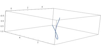
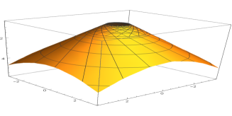
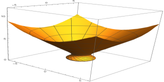
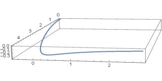
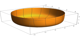
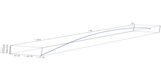
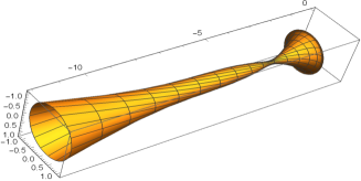
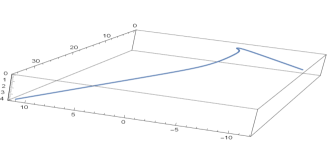
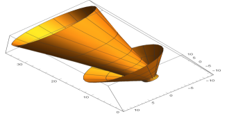
We can give the following example to hold special Smarandache curves in the null cone $\mathbf{Q}^{2}.$ $x\alpha$, $xy$, $\alpha y,$ and $x\alpha y$ special smarandache curves of $x$ curves are given in Figure 1 A, C, E, G, I, respectively. These figures rotated in three dimensions are also given in Figure 1 B, D, F, H, J, respectively.

Example 1.

The curve

$$x(s)=\left(\frac{\cosh s}{2}-\frac{1}{\cosh s},\tanh s,\frac{\cosh s}{2}\right)$$

is spacelike in $\mathbf{Q}^{2}$ with arc length parameter $s$. Also, the shape of the $x$ curve is given as follows

Refer to caption
(a) The curve $x$
Refer to caption
(b) The rotated surface of curve $x$
Refer to caption
(c) $x\alpha-$smarandache curve
Refer to caption
(d) $x\alpha$- smarandache surface.
Refer to caption
(e) $xy-$smarandache curve
Refer to caption
(f) $xy-$smarandache surface.
Refer to caption
(g) $\alpha$y$-$smarandache curve.
Refer to caption
(h) $\alpha$y$-$smarandache surface.
Refer to caption
(i) $x\alpha$y$-$smarandache curve.
Refer to caption
(j) $x\alpha$y$-$smarandache surface.
Figure 1.

Then we can write the smarandache curves of the $x$-curve as follows:

i) $x\alpha-$ smarandache curve $\gamma_{x\alpha}$ is given by

$$\gamma_{x\alpha}(s)=\left(\begin{array}[c]{c}d\left(\frac{\cosh s}{2}-\frac{1}{\cosh s}\right)+\frac{\sinh s}{2}-\frac{\tanh s}{\cosh s},\\ d\tanh s+\frac{1}{\cosh^{2}s},\\ d\frac{\cosh s}{2}+\frac{\sinh s}{2}\end{array}\right)$$

ii) Β x​yβˆ’limit-fromπ‘₯𝑦xy- smarandache curve $\gamma_{xy}$ is given by

Ξ³x​y​(s)=(m​cosh⁑sβˆ’n​tanh⁑s​sinh⁑sβˆ’d​(1​c+tanh2⁑scosh⁑s),c​tanh⁑s​(eβˆ’tanh2⁑s2),d​((cβˆ’tanh2⁑s2)​cosh⁑s2βˆ’1cosh⁑s))subscript𝛾π‘₯π‘¦π‘ π‘šπ‘ π‘›π‘ π‘ π‘‘1𝑐superscript2𝑠𝑠𝑐𝑠𝑒superscript2𝑠2𝑑𝑐superscript2𝑠2𝑠21𝑠\gamma_{xy}(s)=\left(\begin{array}[c]{c}m\cosh s-n\tanh s\sinh s-d\left(\frac{1c+\tanh^{2}s}{\cosh s}\right),\\ c\tanh s\left(e-\frac{\tanh^{2}s}{2}\right),\\ d\left(\left(c-\frac{\tanh^{2}s}{2}\right)\frac{\cosh s}{2}-\frac{1}{\cosh s}\right)\end{array}\right)

iii) $\alpha y-$ smarandache curve $\gamma_{\alpha y}$ is given by

$$\gamma_{\alpha y}(s)=\left(\begin{array}[c]{c}\left(\frac{\cosh s}{2}-\frac{1}{\cosh s}\right)\left(1-e\tanh s\right)\tanh s+\sinh s\left(1+d\tanh s\right)\\ -d\cosh s,\\ -\tanh^{2}s\left(1+d\tanh s\right)+d\tanh s,\\ \frac{\sinh s}{2}-d\cosh s-e\sinh s\tanh s\end{array}\right)$$

iv) $x\alpha y-$ smarandache curve $\gamma_{x\alpha y}$ is given by

Ξ³x​α​y​(s)=(m​sinh⁑sβˆ’n​cosh⁑s+d​sinh⁑s​tanh⁑sβˆ’ccosh⁑sβˆ’b​sinh⁑sβˆ’cβˆ—β€‹tanh2⁑scosh2⁑s,m+n​tanh⁑s+k​tanh2⁑s+l​tanh3⁑s,m​cosh⁑s+d​sinh⁑s+c​tanh⁑s​sinh⁑s,)subscript𝛾π‘₯π›Όπ‘¦π‘ π‘šπ‘ π‘›π‘ π‘‘π‘ π‘ π‘π‘ π‘π‘ superscriptπ‘βˆ—superscript2𝑠superscript2π‘ π‘šπ‘›π‘ π‘˜superscript2𝑠𝑙superscript3π‘ π‘šπ‘ π‘‘π‘ π‘π‘ π‘ \gamma_{x\alpha y}(s)=\left(\begin{array}[c]{c}m\sinh s-n\cosh s+d\sinh s\tanh s-\frac{c}{\cosh s}-\frac{b\sinh s-c^{\ast}\tanh^{2}s}{\cosh^{2}s},\\ m+n\tanh s+k\tanh^{2}s+l\tanh^{3}s,\\ m\cosh s+d\sinh s+c\tanh s\sinh s,\end{array}\right)

where $m,n,d,c,k,l,e\in\mathbb{R}_{0}^{+}.$

References

  • [1] Abdel-Aziz, H.S., Saad, M.K., Smarandache Curves of Some Special Curves in the Galilean $3-$Space, Honan Mathematical J., 37(2), 253-264, 2015.
  • [2] Ali, A.T., ” Special Smarandache Curves in the Euclidean Space”, International Journal of Mathematical Combinatorics, vol.2, 30-36, 2010.
  • [3] Ali, A.T., Time-like Smarandache Curves Derived from a Space-like Helix, Journal of Dynamical Systems and Geometric Theories, 8(1), 93-100, 2010.
  • [4] Ashbacher, C., Smarandache Geometries, Smarandache Notions Journal, 8(1-3), 212-215, 1997.
  • [5] Bayrak, N., Bektas, O. and Yuce, S., Special Smarandache Curves in $\mathbb{R}_{1}^{3}$, Commun. Fac. Sci. Univ. Ank. Ser. A1 Math. Stat., 65(2), 143-160, 2016.
  • [6] Bektas, O. and Yuce, S., ”Special Smarandache Curves According to Darboux Frame in $E^{3}$”, Romanian Journal of Mathematics and Computer Science, 3(1),48-59, 2013.
  • [7] Cetin, M., Kocayiğit, H., On the Quaternionic Smarandache Curves in Euclidean $3-$Space, 8(3),139-150, 2013.
  • [8] Cetin, M., Tuncer, Y., Karacan, M.K., Smarandache Curves According to Bishop Frame in Euclidean $3-$Space, Gen. Math. Notes, 20(2), 50-66, 2014.
  • [9] Elzawy, M., Mosa, S., Smarandache Curves in the Galilean $4-$Space $G_{4}$, Journal of the Egyptian Math. Soc., 25, 53–56, 2017.
  • [10] Kahraman, T., Ugurlu, H.H., Dual Smarandashe Curves and Smarandache Ruled Surfaces, Mathematical Sciences and Applications E-Notes, 2(1), 83-98,2014.
  • [11] Kahraman, T., Ugurlu, H.H., Smarandache Curves of a Spacelike Curve Lying on Unit Dual Lorentzian Sphere $\widetilde{S}_{1}^{2}$, CBU J. of Sci., 11(2), 93-105, 2015.
  • [12] Korpinar, T., Turhan, E., Smarandache $\pi_{1}\pi_{2}$ Curves of Biharmonic New Type Constant $\pi_{2}-$Slope Curves According to type$-2$ Bishop Frame in the Sol Space GDL${}^{3},$ Acta Universitatis Apulensis, No.35, 245-249, 2013.
  • [13] Korpinar, T., New type Surfaces in terms of $B-$Smarandache Curves in $Sol^{3}$, Acta Scientiarum Technology, 37(3), 389-393, 2015.
  • [14] Korpinar, T., Turhan, E., A New Characterization of Smarandache $ts\alpha$ Curves According to Sabban Frame in Heisenberg Group $Heis^{3},$ Int. J. Open Problems Compt. Math., 5(4), 147-155, 2012.
  • [15] Kulahci, M., Bektas, M., ErgΓΌt, M., Curves of AW(k)-Type in 3-Dimensional Null Cone, Physics Letters A 371, 275-277, 2007.
  • [16] Kulahci, M., Almaz, F., Some Characterizations of Osculating in the Lightlike Cone, Bol. Soc. Paran. Math., 35(2), 39-48, 2017.
  • [17] Liu, H., Curves in the Lightlike Cone, Contribbutions to Algebra and Geometry, 45 (1), 291-303, 2004.
  • [18] Liu, H., Meng, Q., Representation Formulas of Curves in a Two- and Three-Dimensional Lightlike Cone, Results Math. 59, 437-451, 2011.
  • [19] Mak, M., Altinbas, H., Spacelike Smarandache Curves of a Timelike Curves in Anti de Sitter 3-Space, International J. Math. Combin., Vol.3, 1-16,2016.
  • [20] O’Neill, B., ”Semi-Riemannian Geometry with Applications to Relativity”, Academic Press, London, 1983.
  • [21] Ozturk, U. and Ozturk, E.B.K., ” Smarandache Curves According to Curves on Spacelike Surface in Minkowski $3-$Space $\mathbb{R}_{1}^{3}$”, Journal of Discrete Mathematics, vol. 2014, article ID829581, 10 pages, 2014.
  • [22] Ozturk, U. and Ozturk, E.B.K., Ilarslan, K., Nesovic, E., On Smarandache Curves Lying in Lightcone in Minkowski $3-$Space, Journal of Dynamical Systems and Geometric Theories, 12(1), 81-91, 2014.
  • [23] Savas, M., Yakut, A.T., Tamirci, T., The Smarandache Curves on $H_{0}^{2}$, Gazi University Journal of Science, 29(1), 69-77, 2016.
  • [24] Senyurt, S., CalΔ±skan, A., Celik, U., $N^{\ast}C^{\ast}$-Smarandache Curves of Bertrand Curves Pair According to Frenet Frame, International J. Math. Combin., 1, 1-7,2016.
  • [25] Senyurt, S., Cevahir, C., Altun, Y., On Spatial Quaternionic Involute Curve a New View, Advances in Applied Clifford Algebras, DOI: 10.1007/s00006-016-0669-7, 2016.
  • [26] Senyurt, S., CalΔ±skan, A., Smarandache Curves in Terms of Sabban Frame of Fixed Pole Curve, Bol. Soc. Paran. Math., 34(2), 53-62, 2016.
  • [27] Senyurt, S., CalΔ±skan, A., Smarandache Curves in Terms of Sabban Frame of Spherical Indicatrix Curves, Gen. Math. Notes, 31(2), 1-15, 2015.
  • [28] Taskopru, K. and Tosun, M., ”Smarandache Curves on $S^{2}$”, Boletim da Sociedade Paranaense de Matematica, 32(1), 51-59, 2014.
  • [29] Turgut, M. and Yilmaz, S., Smarandache Curves in Minkowski Spacetime, International Journal of Mathematical Combinatorics, vol.3, 51-55, 2008.
  • [30] Turhan, E., Korpinar, T., On Smarandache $ts$ Curves of Biharmonic $s$-Curves According to Sabban Frame in Heisenberg group $Heis^{3},$ Advances Modeling and Optimization, 14(2), 343-349, 2012.
  • [31] Yilmaz, S., Unluturk, Y., A Note on Β Spacelike Curves According to Type$-2$ Bishop Frame in Minkowski $3-$Space $E_{1}^{3},$ International Journal of Pure and Applied Mathematics, 103(2), 321-332, 2015.
  • [32] Yilmaz, S., SavcΔ±, U.Z., Smarandache Curves and Applications According to Type$-2$ Bishop Frame in Euclidean $3-$Space, Int. J. Math. Combin. Vol.2, 1-15, 2016.