A structure-preserving split finite element discretization of the split 1D wave equations

Abstract

We introduce a new finite element (FE) discretization framework applicable for covariant split equations. The introduction of additional differential forms (DF) that form pairs with the original ones permits the splitting of the equations into topological momentum and continuity equations and metric-dependent closure equations that apply the Hodge-star operator. Our discretization framework conserves this geometrical structure and provides for all DFs proper FE spaces such that the differential operators (here gradient and divergence) hold in strong form. We introduce lowest possible order discretizations of the split 1D wave equations, in which the discrete momentum and continuity equations follow by trivial projections onto piecewise constant FE spaces, omitting partial integrations. Approximating the Hodge-star by nontrivial Galerkin projections (GP), the two discrete metric equations follow by projections onto either the piecewise constant (GP0) or piecewise linear (GP1) space.

Out of the four possible realizations, our framework gives us three schemes with significantly different behavior. The split scheme using twice GP1 is unstable and shares the dispersion relation with the P1–P1 FE scheme that approximates both variables by piecewise linear spaces (P1). The split schemes that apply a mixture of GP1 and GP0 share the dispersion relation with the stable P1–P0 FE scheme that applies piecewise linear and piecewise constant (P0) spaces. However, the split schemes exhibit second order convergence for both quantities of interest. For the split scheme applying twice GP0, we are not aware of a corresponding standard formulation to compare with. Though it does not provide a satisfactory approximation of the dispersion relation as short waves are propagated much too fast, the discovery of the new scheme illustrates the potential of our discretization framework as a toolbox to study and find FE schemes by new combinations of FE spaces.

Keywords.

Split linear wave equations, Split finite element method, Dispersion relation, Structure-preserving discretization, Shallow-water wave equation

2010 MSC.

76M10 (Primary), 65M60 (Secondary)

1 Introduction

The Finite Element (FE) method provides a powerful framework to discretize partial differential equations (PDEs) and includes methods to prove the discrete models’ convergence, stability, and accuracy properties (see e.g. [8, 20]). By offering flexibility in the choice of computational (unstructured, h/p-adapted) meshes (cf. [6]) while providing an approximation of the continuous PDEs with the required order of accuracy, FE discretizations are nowadays appreciated in all research areas that apply numerical modeling.

Discretizations using finite element methods provide one important advantage over other methods: Starting from a variational formulation the discretization follows simply by substituting the continuous by discrete function spaces (Galerkin methods) while the differential operators remain unchanged. There exist a large variety of different suitable FE spaces to choose from. However, not all choices lead to well-behaving schemes. In particular mixed FE schemes suffer from this problem, where different variables of the PDE system are represented by different FE spaces. In such schemes, certain combinations of FE spaces lead to instabilities that exhibit spurious modes, rendering the solutions useless, in particular when studying nonlinear phenomena. A famous example for an unstable scheme is given by an approximation of both velocity and height fields of the 1D shallow-water equations by piecewise linear functions (cf. [23] and Sect. 3), where it is well known that equal order FE pairs are always unstable [10].

In order to avoid unsuitable choices, the Finite Element Exterior Calculus (FEEC) method [2, 3] provides means for choosing a suitable pair of FE spaces that is guaranteed to lead to a stable mixed discretization. In particular, FEEC puts geometrical constraints on the FE spaces such that geometric properties, like the Helmholtz decomposition of vector-fields, are preserved in the discrete case. As a result, FEEC pairs of spaces always satisfy the inf-sup condition [1] while combinations of FE spaces that are not stable are ruled out. For the above mentioned 1D wave equations, approximating the velocity with piecewise linear and the height field with piecewise constant spaces satisfies the requirements of FEEC and gives indeed a stable scheme (cf. again [23] and Sect. 3).

Although providing a very general mathematical framework, naturally there are issues for which FEEC yields no satisfying answers. Let us consider, for instance, problems in geophysical fluid dynamics (GFD), in which an additional Coriolis term in the equations considers effects caused by the earth’s rotation [22]. For an atmosphere in rest, the Coriolis force that depends on the velocity and the gradient of the pressure (or height) are in geostrophic balance. To maintain this balance in the discretization, the pressure (or height) field should be represented discretely at one order of consistency higher than that of the velocity field. Unfortunately, this contradicts the requirement imposed by FEEC on this FE pair. In [10], this issue could be resolved by applying a combination of FE and Discontinuous Galerkin (DG) spaces.

Moreover, in order to meet the regularity requirement of the chosen FE pairs, FEEC requires the PDEs to be written in weak variational form, in which partial integration has been performed. As pointed out recently in [15], the conventional mixed (weak) form of the equations causes certain operators, such as the co-derivative, to be non-local (global) operators. As a consequence, such FEEC methods are not locally volume preserving, which reduces the quality of the local representation of the quantities of interest (cf. [15]).

In this manuscript our main goal is to introduce a FE discretization framework that provides an alternative methodology to avoid mentioned unsuitable FE choices with GFD in mind. More specifically, we develop a framework that applies two FEEC pairs instead of one, therefore providing a larger variety of different combinations of FE spaces, in which both derivatives and co-derivatives are local operators. This framework is based on formulating the PDEs in split form, as introduced in [4, 5] for the GFD equations. The split equations consist of a topological and metric part while employing straight and twisted differential forms to adequately model the physical quantities of interest. The FE discretization framework translates this geometrical structure from the continuous to similarly structured discrete equations (cf. Sect. 2).

Our approach shares some basic ideas with other discretization techniques, in particular mimetic discretizations (see e.g. [9, 7, 13], and [21] for a historical overview). There, the PDEs are also formulated by differential forms and a clear distinction between purely topological and metric terms is achieved. Applying algebraic topology as discrete counterpart to differential geometry, the discrete equations mimic the underlying geometrical structure and are therefore denoted as structure-preserving (cf. [14]). Similar ideas of distinguishing between metric-dependent and metric-free terms in a GFD related context can also be found in [12] introducing FEEC discretizations of the nonlinear rotating shallow-water equations. In spite of these similarities, none of the schemes associate a proper FE space to each variable, as suggested by our framework.

For the sake of a clear exposition, we focus on a simple example, the split 1D linear shallow-water set of equations. Extending our framework to treat also more practically relevant equations, such as the nonlinear rotating shallow-water equations, is subject of ongoing and future work. By investigating structure-preserving methods that apply lowest order (piecewise linear and constant) FE spaces to keep computational costs low, we address the requirements of GFD in developing schemes that satisfy first principle conservation laws (i.e mass and momentum conservation) and that are suited for simulations with integration times in the order of years and longer.

We structure the manuscript as follows. In Sect. 2, we introduce the split set of 1D wave equations and motivate the use of the split form of equations as principle formulation for their discretization. Recalling in Sect. 3 two low-order mixed FE schemes, namely the unstable P1–P1 and the stable P1–P0 pairs, we introduce in Sect. 4 the new discretization framework, referred to as split FE method. We suggest a solving algorithm and present the schemes’ discrete dispersion relations. Comparing them if possible with the conventional mixed schemes, we perform in Sect. 5 numerical simulations to investigate conservation behavior, convergence rates, and accuracy of all schemes. Finally in Sect. 6, we draw conclusions and provide an outlook for ongoing and future work.

2 Hierarchical structuring of the wave equation

In order to convey the basic ideas to the reader most clearly and comprehensively, we develop our FE discretization framework on a simple example, the set of 1D wave equations. As the split form of the equations (cf. [5]) is an essential ingredient of our approach, we first introduce the corresponding split 1D wave equations and compare them with conventional formulations.

A hierarchical structuring of the wave equation.

Compared to conventional formulations, the split 1D wave equations arrange themselves in the following hierarchy of linear wave equations:

1. one $2^{\rm nd}$-order equation:

   $$\frac{\partial^{2}h(x,t)}{\partial t^{2}}-c^{2}\frac{\partial^{2}h(x,t)}{\partial x^{2}}=0,$$ (1)

   with phase velocity $c=\omega/k$ for wave frequency $\omega$ and wave number $k$ and with boundary condition (BC) $h(0,t)=h(L,t)\,\forall t$;

2. two $1^{\rm st}$-order equations:

   $$\frac{\partial u(x,t)}{\partial t}+g\frac{\partial h(x,t)}{\partial x}=0,\qquad\frac{\partial h(x,t)}{\partial t}+H\frac{\partial u(x,t)}{\partial x}=0,$$ (2)

   with phase velocity $c=\sqrt{gH}$ and BCs $h(0,t)=h(L,t),\,u(0,t)=u(L,t)\,\forall t$;

3. two $1^{\rm st}$-order equations and two closure equations:

   $$\begin{split}\frac{\partial u^{(1)}}{\partial t}+g{\bf d}h^{(0)}=0,&\qquad\frac{\partial\widetilde{h}^{(1)}}{\partial t}+H{\bf d}\widetilde{u}^{(0)}=0,\\ \widetilde{u}^{(0)}=\widetilde{\star}u^{(1)},&\qquad\widetilde{h}^{(1)}=\widetilde{\star}h^{(0)},\end{split}$$ (3)

   with phase velocity $c=\sqrt{gH}$ and BCs $h^{(0)}(0,t)=h^{(0)}(L,t),\,\widetilde{u}^{(0)}(0,t)=\widetilde{u}^{(0)}(L,t)\,\forall t$;

for a periodic domain $x\in[0,L]$. The smooth function $h(x,t)$ denotes the height elevation with mean fluid height $H$ while assuming a trivial bottom topography. The smooth function $u(x,t)$ denotes the velocity of some fluid parcel in direction of $x$ at time $t\in[0,T]\subset\mathbbm{R}$. $g$ is the gravitational acceleration. Describing the momentum and height of a shallow water column, equations (2) are usually referred to as shallow-water equations. Throughout this manuscript however, we will refer to the preceding formulations as wave equations.

The splitting of equations (3) into topological (first line) and metric parts (second line) is based on their formulation in terms of differential forms: $u^{(1)}\in(\color[rgb]{0,0,0}\Lambda^{1}\color[rgb]{0,0,0};0,T)$ denotes a time-dependent straight 1-form and $h^{(0)}\in(\color[rgb]{0,0,0}\Lambda^{0}\color[rgb]{0,0,0};0,T)$ a time-dependent straight 0-form (straight function) – straight forms do not change their signs when the orientation of the manifold changes; $\widetilde{u}^{(0)}\in(\color[rgb]{0,0,0}\widetilde{\Lambda}^{0}\color[rgb]{0,0,0};0,T)$ denotes a time-dependent twisted 0-form and $\widetilde{h}^{(1)}\in(\color[rgb]{0,0,0}\widetilde{\Lambda}^{1}\color[rgb]{0,0,0};0,T)$ a time-dependent twisted 1-form – twisted forms compensate the change in signs which would result from a change in orientation. The latter property is shared by the twisted Hodge-star operator $\widetilde{\star}:\Lambda^{k}\rightarrow\widetilde{\Lambda}^{(1-k)}$ (resp. $\widetilde{\Lambda}^{k}\rightarrow\Lambda^{(1-k)}$) mapping from straight (resp. twisted) $k$-forms to twisted (resp. straight) $(1-k)$-forms, here for $k=0,1,$ as we are in one dimension. The index ^(k) denotes the degree, and $\Lambda^{k},\widetilde{\Lambda}^{k}$ the space of all $k$-forms.

The exterior derivative is defined as the map ${\bf d}:\color[rgb]{0,0,0}\Lambda^{0}\color[rgb]{0,0,0}\rightarrow\color[rgb]{0,0,0}\Lambda^{1}\color[rgb]{0,0,0}$ (or ${\bf d}:\color[rgb]{0,0,0}\widetilde{\Lambda}^{0}\color[rgb]{0,0,0}\rightarrow\color[rgb]{0,0,0}\widetilde{\Lambda}^{1}\color[rgb]{0,0,0}$ for twisted forms, cf. diagram (25)). It reduces in one dimension to the total derivative of a smooth function $f(x)$, i.e. for $f^{(0)}\in\color[rgb]{0,0,0}\Lambda^{0}\color[rgb]{0,0,0},{\bf d}f^{(0)}=\partial_{x}f(x)dx\in\color[rgb]{0,0,0}\Lambda^{1}\color[rgb]{0,0,0}$. The map of $\bf d$ on twisted forms is defined analogously.

We refer the reader to Sec. 4.1 for an explicit representation of the split wave equations (3) in the local coordinate $x\in[0,L]$, and to [5] for an elaborated discussion about straight and twisted forms, the twisted Hodge-star operators, and the derivation of $n$-dimensional split equations of GFD.

The split wave equations:

We argued in detail in [5] why it is favorable to represent the equations of GFD in terms of differential forms rather than vector-calculus notation, and we discussed advantages of the split form in particular. Here, the split representation of the wave equations fits naturally into the arrangement of wave equations presented above, in which the saddle point (mixed) form (2) results from a splitting of the standard form (1), and the split form (3) from a further splitting of the saddle point form (2). This somehow suggests to study in more detail possible benefits of a discretization based on the split form (3) rather than on the mixed form (2), just as there exist cases in which discretizations based on equations (2), usually discretized by mixed FE methods, perform better than schemes resulting from standard FE approaches that rely on formulation (1).

Let us first elaborate on the latter point, for which we present two examples where standard FE schemes even fail to provide correct solutions. As pointed out in [3], the standard FE solution to the vector Poisson equation on non-convex polyhedral domains will converge to a false solution of the problem for almost all forcing functions $f$. The same happens when calculating standard FE solutions for the vector Laplacian on an annulus. However, correct solutions can be obtained when using mixed formulations, in particular those based on FEEC [3]. In addition, mixed formulations, in which two or even more FE spaces are used to approximate separate variables, are well suited for saddle point problems. These arise, for instance, in constrained minimization problems (Stokes equations or Darcy flow), in which the elimination of one of the variables is not possible (cf. [20], Chapter 36). In this latter case, equations in form (1) do even not exist. There are also some physical and numerical reasons in favor of mixed FE methods. According to [18], it is the first-order system, such as (2), that follows from physics (i.e. from first conservation principles of mass and momentum) and not the second-order equation, such as (1). In particular, efficient numerical schemes can be derived more easily from the first-order system.

Following in particular the latter line of argumentation, the split form more accurately models the physical properties than the first-order system, because system (3) provides for each variable the adequate (straight or twisted) differential form that suits in dimension and orientation the corresponding property of a real fluid (cf. [5], Section 7). It seems appropriate during the discretization process to provide for each variable a suitable FE space too. As a proof of concept, one aim of this manuscript is to exploit this additional freedom in the choice of FE spaces and study, in terms of convergence, accuracy, stability and dispersion relation, possible advantages, but also drawbacks, that come along with this generalized FE method.

More precisely, by using the split form of the equations, we approximate each variable by a FE space such that the discrete version of the exterior derivative $\bf d$ satisfies the mappings $\Lambda_{h}^{0}\rightarrow\Lambda_{h}^{1}$ and $\widetilde{\Lambda}_{h}^{0}\rightarrow\widetilde{\Lambda}_{h}^{1}$. $\Lambda_{h}^{i},\widetilde{\Lambda}_{h}^{i},i=0,1$, are FE spaces that approximate the corresponding continuous spaces. As pointed out later in more detail, this approach guarantees correct discrete topological equations up to projection error caused by projecting the continuous equations into the FE spaces. Any additional errors are caused by the metric-dependent closure equations that are realized by nontrivial projections between straight and twisted spaces (cf. Sect. 4). Such a clear separation between projection and additional errors, the latter caused by partial integrations in the weak form, is not obvious in mixed FE methods. Part of future work will be to study how these different error sources relate.

3 The mixed finite element method

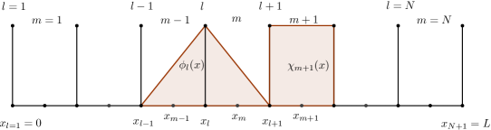
Figure 1: Discretization of the periodic domain $x\in[0,L]$ by $N$ subintervals (elements) and $N$ independent nodes; the former are denoted by $m$, the latter by $l$ for $m,l=1,..,N$. $\color[rgb]{0,0,0}\phi_{l}(x)\color[rgb]{0,0,0}$ are the basis functions of $\color[rgb]{0,0,0}V^{1}_{h}\color[rgb]{0,0,0}$ and $\color[rgb]{0,0,0}\chi_{m}(x)\color[rgb]{0,0,0}$ of $\color[rgb]{0,0,0}V^{0}_{h}\color[rgb]{0,0,0}$ (cf. Appendix A for their definition).

In this section, we briefly review two examples of the general idea behind mixed FE methods and we introduce notations and definitions required for the remainder of the paper. First, we observe that there are two equations for two prognostic variables in equation (2). In order to discretize them one has the choice of mixing the corresponding FE spaces, which gives rise to the naming convention. Here we consider (i) similar $(\color[rgb]{0,0,0}V^{1}_{h}\color[rgb]{0,0,0},\color[rgb]{0,0,0}V^{1}_{h}\color[rgb]{0,0,0},)$ or (ii) mixed FE spaces $(\color[rgb]{0,0,0}V^{1}_{h}\color[rgb]{0,0,0},\color[rgb]{0,0,0}V^{0}_{h}\color[rgb]{0,0,0})$, where $\color[rgb]{0,0,0}V^{1}_{h}\color[rgb]{0,0,0}$ refers to a linear and $\color[rgb]{0,0,0}V^{0}_{h}\color[rgb]{0,0,0}$ to a constant FE space.

In more detail, we subdivide the domain $[0,L]$ into $N$ subintervals $[x_{l},x_{l+1}]$, for $l=1,\dots N,$ as shown in Figure 1. We denote the points $x_{l}$ as nodes $l$ and the subintervals as elements $m$ with centers $x_{m}:=\frac{1}{2}(x_{l}+x_{l+1})$ and element sizes $\Delta x_{m}=(x_{l+1}-x_{l})$, for $l,m=1,\dots N$. Basis functions and coefficients at nodes carry the subindices $l$ and $l^{\prime}$ and those at element centers the subindices $m$ and $m^{\prime}$. To impose periodic boundary conditions, we identify the nodes at $x=0$ and at $x=L$ with each other and consider only 1 Degree of Freedom (DoF) associated to this node. We have thus $N$ independent DoF for both nodes and elements.

Throughout this manuscript we will use the Lagrange functions $\{\color[rgb]{0,0,0}\phi_{l}(x)\color[rgb]{0,0,0}\}_{{\color[rgb]{0,0,0}{l}\color[rgb]{0,0,0}}=1}^{N}$ as basis for the piecewise linear FE space $\color[rgb]{0,0,0}V^{1}_{h}\color[rgb]{0,0,0}$ and the step functions $\{\color[rgb]{0,0,0}\chi_{m}(x)\color[rgb]{0,0,0}\}_{{\color[rgb]{0,0,0}{m}\color[rgb]{0,0,0}}=1}^{N}$ as basis for the piecewise constant FE space $\color[rgb]{0,0,0}V^{0}_{h}\color[rgb]{0,0,0}$ (cf. Appendix A for their definitions).

3.1 The unstable P1–P1 finite element discretization

In order to find approximate solutions of the wave equations (2), we apply Galerkin’s method. To this end, we formulate the wave equations in variational form and approximate $u(x,t)$ and $h(x,t)$ by suitable discrete functions. Being aware of the problems of spurious modes (discussed below), we start with a naive choice of a pair of FE spaces approximating both $u(x,t)$ and $h(x,t)$ by piecewise linear (P1) functions $u_{h}(x,t)\in(\color[rgb]{0,0,0}V^{1}_{h}\color[rgb]{0,0,0};0,T)$ and $h_{h}(x,t)\in(\color[rgb]{0,0,0}V^{1}_{h}\color[rgb]{0,0,0};0,T)$. We refer to this scheme as P1–P1 scheme.

The discrete variational form of the wave equations is then given by: find $(u_{h}(x,t),h_{h}(x,t))\in(\color[rgb]{0,0,0}V^{1}_{h}\color[rgb]{0,0,0};0,T)\times(\color[rgb]{0,0,0}V^{1}_{h}\color[rgb]{0,0,0};0,T)$, such that

$$\begin{split}\int_{L}\left(\frac{\partial u_{h}(x,t)}{\partial t}+g\frac{\partial h_{h}(x,t)}{\partial x}\right)\hat{\phi}(x)dx&=0,\quad\forall\hat{\phi}(x)\in\color[rgb]{0,0,0}\hat{V}^{1}_{h}\color[rgb]{0,0,0}\subset\color[rgb]{0,0,0}V^{1}\color[rgb]{0,0,0},\qquad\\ \int_{L}\left(\frac{\partial h_{h}(x,t)}{\partial t}+H\frac{\partial u_{h}(x,t)}{\partial x}\right)\hat{\phi}(x)dx&=0,\quad\forall\hat{\phi}(x)\in\color[rgb]{0,0,0}\hat{V}^{1}_{h}\color[rgb]{0,0,0}\subset\color[rgb]{0,0,0}V^{1}\color[rgb]{0,0,0},\end{split}$$ (4)

for any test function $\hat{\phi}(x)$ in the test space $\color[rgb]{0,0,0}\hat{V}^{1}_{h}\color[rgb]{0,0,0}$. Expanding the variables in terms of the basis of the trial space $\color[rgb]{0,0,0}V^{1}_{h}\color[rgb]{0,0,0}$,

$${u}_{h}(x,t)\approx\sum_{{\color[rgb]{0,0,0}{l}\color[rgb]{0,0,0}}=1}^{N}\color[rgb]{0,0,0}u_{l}\color[rgb]{0,0,0}(t)\color[rgb]{0,0,0}\phi_{l}(x)\color[rgb]{0,0,0}\,\quad\text{and}\quad{h}_{h}(x,t)\approx\sum_{{\color[rgb]{0,0,0}{l}\color[rgb]{0,0,0}}=1}^{N}\color[rgb]{0,0,0}h_{l}\color[rgb]{0,0,0}(t)\color[rgb]{0,0,0}\phi_{l}(x)\color[rgb]{0,0,0}\,,$$ (5)

with time dependent coefficients $\color[rgb]{0,0,0}u_{l}\color[rgb]{0,0,0}(t)$ and $\color[rgb]{0,0,0}h_{l}\color[rgb]{0,0,0}(t)$, and varying the test functions $\hat{\phi}(x)$ over the basis functions $\{\color[rgb]{0,0,0}\phi_{l^{\prime}}(x)\color[rgb]{0,0,0}\}_{{\color[rgb]{0,0,0}{l^{\prime}}\color[rgb]{0,0,0}}=1}^{N}$ of the test space $\color[rgb]{0,0,0}\hat{V}^{1}_{h}\color[rgb]{0,0,0}$, we obtain

$$\begin{split}\sum_{{\color[rgb]{0,0,0}{l}\color[rgb]{0,0,0}}=1}^{N}\partial_{t}\color[rgb]{0,0,0}u_{l}\color[rgb]{0,0,0}(t)\int_{L}\color[rgb]{0,0,0}\phi_{l}(x)\color[rgb]{0,0,0}\color[rgb]{0,0,0}\phi_{l^{\prime}}(x)\color[rgb]{0,0,0}dx+g\sum_{{\color[rgb]{0,0,0}{l}\color[rgb]{0,0,0}}=1}^{N}\color[rgb]{0,0,0}h_{l}\color[rgb]{0,0,0}(t)\int_{L}\frac{d\color[rgb]{0,0,0}\phi_{l}(x)\color[rgb]{0,0,0}}{dx}\color[rgb]{0,0,0}\phi_{l^{\prime}}(x)\color[rgb]{0,0,0}dx=0,\quad\text{\ for\ }{\color[rgb]{0,0,0}{l^{\prime}}\color[rgb]{0,0,0}}=1,\dots,N,\\ \sum_{{\color[rgb]{0,0,0}{l}\color[rgb]{0,0,0}}=1}^{N}\partial_{t}\color[rgb]{0,0,0}h_{l}\color[rgb]{0,0,0}(t)\int_{L}\color[rgb]{0,0,0}\phi_{l}(x)\color[rgb]{0,0,0}\color[rgb]{0,0,0}\phi_{l^{\prime}}(x)\color[rgb]{0,0,0}dx+H\sum_{{\color[rgb]{0,0,0}{l}\color[rgb]{0,0,0}}=1}^{N}\color[rgb]{0,0,0}u_{l}\color[rgb]{0,0,0}(t)\int_{L}\frac{d\color[rgb]{0,0,0}\phi_{l}(x)\color[rgb]{0,0,0}}{dx}\color[rgb]{0,0,0}\phi_{l^{\prime}}(x)\color[rgb]{0,0,0}dx=0,\quad\text{\ for\ }{\color[rgb]{0,0,0}{l^{\prime}}\color[rgb]{0,0,0}}=1,\dots,N.\end{split}$$ (6)

This discrete system can analogously be written in matrix-vector formulation. Defining the coefficient vectors $\color[rgb]{0,0,0}{\bf u}_{n}\color[rgb]{0,0,0}=(u_{1}(t),...,u_{l}(t),...,u_{N}(t))$ and $\color[rgb]{0,0,0}{\bf h}_{n}\color[rgb]{0,0,0}=(h_{1}(t),...,h_{l}(t),...,h_{N}(t))$, with subindex $n$ for nodes, we obtain the following linear system of algebraic equations:

$${\bf M}^{nn}\frac{\partial\color[rgb]{0,0,0}{\bf u}_{n}\color[rgb]{0,0,0}}{\partial t}+g{\bf D}^{nn}\color[rgb]{0,0,0}{\bf h}_{n}\color[rgb]{0,0,0}=0,\quad{\bf M}^{nn}\frac{\partial\color[rgb]{0,0,0}{\bf h}_{n}\color[rgb]{0,0,0}}{\partial t}+H{\bf D}^{nn}\color[rgb]{0,0,0}{\bf u}_{n}\color[rgb]{0,0,0}=0,$$ (7)

in which ${\bf M}^{nn}$ is a $(N\times N)$ mass-matrix with metric-dependent coefficient

$$M_{{\color[rgb]{0,0,0}{l}\color[rgb]{0,0,0}}{\color[rgb]{0,0,0}{l^{\prime}}\color[rgb]{0,0,0}}}=\int_{L}\color[rgb]{0,0,0}\phi_{l}(x)\color[rgb]{0,0,0}\color[rgb]{0,0,0}\phi_{l^{\prime}}(x)\color[rgb]{0,0,0}dx,$$ (8)

and ${\bf D}^{nn}$ a $(N\times N)$ stiffness-matrix with metric-independent coefficients

$$D_{{\color[rgb]{0,0,0}{l}\color[rgb]{0,0,0}}{\color[rgb]{0,0,0}{l^{\prime}}\color[rgb]{0,0,0}}}=\int_{L}\frac{d\color[rgb]{0,0,0}\phi_{l}(x)\color[rgb]{0,0,0}}{dx}\color[rgb]{0,0,0}\phi_{l^{\prime}}(x)\color[rgb]{0,0,0}dx\,.$$ (9)

In Appendix A, we provide explicit representations of these matrices for the mesh of Figure 1 subject to periodic boundary conditions.

Time discretization.

To discretize the semi-discrete equations (7) in time, we use the Crank-Nicolson (CN) scheme, a symmetric, implicit time discretization method. Then, for the time $t\in[0,T]$ and a time step size of $\Delta t$, the full discretized matrix-vector equations read

$${\bf M}^{nn}\color[rgb]{0,0,0}{\bf u}_{n}\color[rgb]{0,0,0}{}^{t+1} ={\bf M}^{nn}\color[rgb]{0,0,0}{\bf u}_{n}\color[rgb]{0,0,0}{}^{t}+\frac{1}{2}\Delta tg{\bf D}^{nn}\color[rgb]{0,0,0}{\bf h}_{n}\color[rgb]{0,0,0}{}^{t}+\frac{1}{2}\Delta tg{\bf D}^{nn}\color[rgb]{0,0,0}{\bf h}_{n}\color[rgb]{0,0,0}{}^{t+1},$$ (10)

$${\bf M}^{nn}\color[rgb]{0,0,0}{\bf h}_{n}\color[rgb]{0,0,0}{}^{t+1} ={\bf M}^{nn}\color[rgb]{0,0,0}{\bf h}_{n}\color[rgb]{0,0,0}{}^{t}+\frac{1}{2}\Delta tH{\bf D}^{nn}\color[rgb]{0,0,0}{\bf u}_{n}\color[rgb]{0,0,0}{}^{t}+\frac{1}{2}\Delta tH{\bf D}^{nn}\color[rgb]{0,0,0}{\bf u}_{n}\color[rgb]{0,0,0}{}^{t+1}.$$ (11)

We will solve these equations by fixed point iteration, even though they could be solved directly due to the linearity. The motivation for this inefficient algorithmic choice lies in future work on non-linear equations and the possibility to treat possible kernels for the discrete Hodge-star operators in the split schemes (cf. (43)). For more details on the solver, we refer to Sect. 4.3 in which we introduce a corresponding algorithm for the split finite element schemes.

The choice of using an iterative algorithm does not alter the results discussed in this paper. Only the time step size has to be restricted, in spite of the unconditional stability of the CN scheme. Similarly to the CFL number in explicit schemes, $\Delta t$ must not exceed a certain threshold $\mu$ in order to guarantee that even the fastest waves are sufficiently well resolved and that the iterative solver converges. Defining the CFL number for the 1D wave equations by

$$\mu=\sqrt{gH}\frac{\Delta t}{\Delta x}\,,$$ (12)

we restrict $\Delta t$ for a given $\Delta x$ such that $\mu$ is smaller that some constant. This constant, determined empirically for all test cases and mesh resolutions applied in this manuscript, is given for the unstable scheme by $\mu\leq 1.15$ (see Sect. 4.3 for more details).

Discussion about spatial stability.

Throughout this paper, we study the stability properties of each discrete scheme by investigating whether it supports spurious modes. Such spurious modes are free modes, i.e. unphysical, very oscillatory small-scale waves on the grid scale that are not constrained by the discrete equations. In case of nonlinear equations, these modes get coupled to the smooth solution and grow fast, making the scheme unusable. Besides studying the inf-sup condition (see, e.g. [8]), one way of investigating the occurrence of such spurious modes is to determine the dispersion relation of the discrete scheme.

For the unstable P1–P1 FE scheme, we associate spurious modes with those modes that show zero group velocity $\omega$, for some wave numbers $k$. These modes are trapped to the grid scale and may lead to the just described instabilities. More precisely, the angular frequency $\omega=\omega(k)$ satisfies the dispersion relation (see Appendix B)

$$c_{d}=\frac{\omega}{k}=\pm\sqrt{gH}\frac{\sin(k\Delta x)}{k\Delta x}\left[\frac{3}{2+\cos(k\Delta x)}\right].$$ (13)

For small $k\rightarrow 0$, the discrete dispersion relation converges to the continuous one with $c_{d}\rightarrow c=\sqrt{gH}$. However, besides the correct zero frequency at $k=0$, this dispersion relation has at the shortest wave length $k=\frac{\pi}{\Delta x}$ a second zero solution (spurious mode) with zero wave speed leading to an unphysical standing wave.

3.2 The stable P1–P0 finite element discretization

The instability demonstrated in the previous subsection, caused by a choice of similar FE spaces for both variables, is a general feature of methods with same FE spaces for approximating $u$ and $h$ (cf. [11]). To avoid this problem, we present a stable mixed FE method using different FE spaces to approximate velocity and height.

As proposed by other authors (e.g. [16]), we approximate $u(x,t)$ by the piecewise linear (P1) function $u_{h}(x,t)\in(\color[rgb]{0,0,0}V^{1}_{h}\color[rgb]{0,0,0};0,T)$ and $h(x,t)$ by the piecewise constant (P0) function $h_{h}(x,t)\in(\color[rgb]{0,0,0}V^{0}_{h}\color[rgb]{0,0,0};0,T)$ and we apply Galerkin’s method to find these approximations. We refer to this scheme as P1–P0 scheme.

The formulation of the wave equations (2) in variational form implies multiplication of the momentum equation by a test function $\hat{\phi}(x)\in\color[rgb]{0,0,0}\hat{V}^{1}_{h}\color[rgb]{0,0,0}$ and of the continuity equation by a test function $\hat{\chi}(x)\in\color[rgb]{0,0,0}\hat{V}^{0}_{h}\color[rgb]{0,0,0}$. Because the derivative of $h_{h}(x,t)$ is not well-defined globally, the corresponding term in the momentum equation requires integration by parts, whereas for the remaining terms trivial projections into the corresponding spaces are suitable.

The discrete variational/weak form of the wave equations is thus given by: find $(u_{h}(x,t),h_{h}(x,t))\in(\color[rgb]{0,0,0}V^{1}_{h}\color[rgb]{0,0,0};0,T)\times(\color[rgb]{0,0,0}V^{0}_{h}\color[rgb]{0,0,0};0,T)$, such that

$$\begin{split}\int_{L}\left(\frac{\partial u_{h}(x,t)}{\partial t}\hat{\phi}(x)-gh_{h}(x,t)\frac{\partial\hat{\phi}(x)}{\partial x}\right)dx&=0,\quad\forall\hat{\phi}(x)\in\color[rgb]{0,0,0}\hat{V}^{1}_{h}\color[rgb]{0,0,0}\subset\color[rgb]{0,0,0}V^{1}\color[rgb]{0,0,0},\\ \int_{L}\left(\frac{\partial h_{h}(x,t)}{\partial t}+H\frac{\partial u_{h}(x,t)}{\partial x}\right)\hat{\chi}(x)dx&=0,\quad\forall\hat{\chi}(x)\in\color[rgb]{0,0,0}\hat{V}^{0}_{h}\color[rgb]{0,0,0}\subset\color[rgb]{0,0,0}V^{0}\color[rgb]{0,0,0}.\end{split}$$ (14)

The momentum equation is given in weak form, due to the integration by parts, while the continuity equations remains in variational form. The boundary terms from integration by parts in the weak momentum equation vanish because of the periodic boundary conditions and continuity conditions at cell interfaces. This special treatment is a source of additional error, while the trivially projected terms do not introduce further errors beyond those caused by the approximation of the initial conditions by the FE spaces [11].

Expanding the variables in terms of the corresponding bases yields

$${u}_{h}(x,t)\approx\sum_{{\color[rgb]{0,0,0}{l}\color[rgb]{0,0,0}}=1}^{N}\color[rgb]{0,0,0}u_{l}\color[rgb]{0,0,0}(t)\color[rgb]{0,0,0}\phi_{l}(x)\color[rgb]{0,0,0}\quad\text{and}\quad{h}_{h}(x,t)\approx\sum_{{\color[rgb]{0,0,0}{m}\color[rgb]{0,0,0}}=1}^{N}\color[rgb]{0,0,0}h_{m}\color[rgb]{0,0,0}(t)\color[rgb]{0,0,0}\chi_{m}(x)\color[rgb]{0,0,0}.$$ (15)

Substituting these expansions into equations (14) gives

$$\begin{split}\sum_{{\color[rgb]{0,0,0}{l}\color[rgb]{0,0,0}}=1}^{N}\partial_{t}\color[rgb]{0,0,0}u_{l}\color[rgb]{0,0,0}(t)\int_{L}\color[rgb]{0,0,0}\phi_{l}(x)\color[rgb]{0,0,0}\color[rgb]{0,0,0}\phi_{l^{\prime}}(x)\color[rgb]{0,0,0}dx-g\sum_{{\color[rgb]{0,0,0}{m}\color[rgb]{0,0,0}}=1}^{N}\color[rgb]{0,0,0}h_{m}\color[rgb]{0,0,0}(t)\int_{L}\color[rgb]{0,0,0}\chi_{m}(x)\color[rgb]{0,0,0}\frac{d\color[rgb]{0,0,0}\phi_{l^{\prime}}(x)\color[rgb]{0,0,0}}{dx}dx&=0,\quad\text{\ for\ }{\color[rgb]{0,0,0}{l^{\prime}}\color[rgb]{0,0,0}}=1,\dots,N,\\ \sum_{{\color[rgb]{0,0,0}{m}\color[rgb]{0,0,0}}=1}^{N}\partial_{t}\color[rgb]{0,0,0}h_{m}\color[rgb]{0,0,0}(t)\int_{L}\color[rgb]{0,0,0}\chi_{m}(x)\color[rgb]{0,0,0}\color[rgb]{0,0,0}\chi_{m^{\prime}}(x)\color[rgb]{0,0,0}dx+H\sum_{{\color[rgb]{0,0,0}{l}\color[rgb]{0,0,0}}=1}^{N}\color[rgb]{0,0,0}u_{l}\color[rgb]{0,0,0}(t)\int_{L}\frac{d\color[rgb]{0,0,0}\phi_{l}(x)\color[rgb]{0,0,0}}{dx}\color[rgb]{0,0,0}\chi_{m^{\prime}}(x)\color[rgb]{0,0,0}dx&=0,\quad\text{\ for\ }{\color[rgb]{0,0,0}{m^{\prime}}\color[rgb]{0,0,0}}=1,\dots,N.\end{split}$$ (16)

Analogously to equation (6) this discrete system can be written in matrix-vector formulation. For the coefficient vectors $\color[rgb]{0,0,0}{\bf u}_{n}\color[rgb]{0,0,0}=(u_{1}(t),...,u_{l}(t),...,u_{N}(t))$ with subindex $n$ for nodes and $\color[rgb]{0,0,0}{\bf h}_{e}\color[rgb]{0,0,0}=(h_{1}(t),...,h_{m}(t),...,h_{N}(t))$ with subindex $e$ for elements, we obtain the following linear system

$${\bf M}^{nn}\frac{\partial\color[rgb]{0,0,0}{\bf u}_{n}\color[rgb]{0,0,0}}{\partial t}-g{\bf D}^{ne}\color[rgb]{0,0,0}{\bf h}_{e}\color[rgb]{0,0,0}=0,\quad{\bf M}^{ee}\frac{\partial\color[rgb]{0,0,0}{\bf h}_{e}\color[rgb]{0,0,0}}{\partial t}+H{\bf D}^{en}\color[rgb]{0,0,0}{\bf u}_{n}\color[rgb]{0,0,0}=0.$$ (17)

${\bf M}^{nn}$ is the mass-matrix from above with metric-dependent coefficients (8), ${\bf M}^{ee}$ is a $(N\times N)$ mass-matrix with metric-dependent coefficients

$$M_{{\color[rgb]{0,0,0}{m}\color[rgb]{0,0,0}}{\color[rgb]{0,0,0}{m^{\prime}}\color[rgb]{0,0,0}}}=\int_{L}\color[rgb]{0,0,0}\chi_{m}(x)\color[rgb]{0,0,0}\color[rgb]{0,0,0}\chi_{m^{\prime}}(x)\color[rgb]{0,0,0}dx,$$ (18)

and ${\bf D}^{ne}$ and ${\bf D}^{en}$ are $(N\times N)$ stiffness-matrices. Recall that in 1D with periodic BC, the number of nodes and the number of elements coincide, therefore all matrices are of size $N\times N$. The metric-independent coefficients of ${\bf D}^{en}$ are defined by

$$D_{{\color[rgb]{0,0,0}{l}\color[rgb]{0,0,0}}{\color[rgb]{0,0,0}{m^{\prime}}\color[rgb]{0,0,0}}}=\int_{L}\frac{d\color[rgb]{0,0,0}\phi_{l}(x)\color[rgb]{0,0,0}}{dx}\color[rgb]{0,0,0}\chi_{m^{\prime}}(x)\color[rgb]{0,0,0}dx\,,$$ (19)

and those of ${\bf D}^{ne}$ via the property ${\bf D}^{ne}=({\bf D}^{en})^{T}$, in which $()^{T}$ denotes the transpose of a matrix. We refer to Appendix A to see the full matrices for the example given in Figure 1.

Time discretization.

To discretize the semi-discrete equations (17) in time, we use the Crank-Nicolson scheme again. For the time $t\in[0,T]$ and a time step size of $\Delta t$, the fully discretized matrix-vector equations read

$${\bf M}^{nn}\color[rgb]{0,0,0}{\bf u}_{n}\color[rgb]{0,0,0}{}^{t+1} ={\bf M}^{nn}\color[rgb]{0,0,0}{\bf u}_{n}\color[rgb]{0,0,0}{}^{t}-\frac{1}{2}\Delta tg{\bf D}^{ne}\color[rgb]{0,0,0}{\bf h}_{e}\color[rgb]{0,0,0}{}^{t}-\frac{1}{2}\Delta tg{\bf D}^{ne}\color[rgb]{0,0,0}{\bf h}_{e}\color[rgb]{0,0,0}{}^{t+1},$$ (20)

$${\bf M}^{ee}\color[rgb]{0,0,0}{\bf h}_{e}\color[rgb]{0,0,0}{}^{t+1} ={\bf M}^{ee}\color[rgb]{0,0,0}{\bf h}_{e}\color[rgb]{0,0,0}{}^{t}+\frac{1}{2}\Delta tH{\bf D}^{en}\color[rgb]{0,0,0}{\bf u}_{n}\color[rgb]{0,0,0}{}^{t}+\frac{1}{2}\Delta tH{\bf D}^{en}\color[rgb]{0,0,0}{\bf u}_{n}\color[rgb]{0,0,0}{}^{t+1}.$$ (21)

We solve this implicit system of equations iteratively by fixed point iteration (cf. Sect. 4.3 for more details).

Here, we restrict the time step size such that for all meshes and test cases studied the CFL number (12) satisfies $\mu\leq 0.57$. This is only half the value compared to the unstable P1–P1 scheme, since the lower order representation of the height field leads effectively to a coarsened spatial resolution.

Discussion about spatial stability.

We briefly discuss the stability of the method by studying it’s discrete dispersion relation. As shown in Appendix B, $\omega=\omega(k)$ satisfies the dispersion relation

$$c_{d}=\frac{\omega}{k}=\pm\sqrt{gH}\frac{\sin(k\frac{\Delta x}{2})}{k\frac{\Delta x}{2}}\left[\frac{3}{2+\cos(k\Delta x)}\right]^{1/2}\,.$$ (22)

The discrete wave speed $c_{d}$ converges for $k\rightarrow 0$ to the analytical wave speed $c$ also for the P1–P0 case. However, this relation has only one root for $\omega$ at $k=0$, while it shows a good approximation to the continuous dispersion relation at the shortest wave length $k=\frac{\pi}{\Delta x}$, in contrast to the unstable P1–P1 scheme (cf. Fig. 2). Hence, this scheme exhibits no spurious modes and is therefore stable.

4 The split finite element method

In this section, we introduce a new finite element discretization method that uses the split formulation of the wave equations (3) (cf. [5] for a more general formulation of such split equations). It is referred to in the following as split finite element (FE) method.

The split FE method is based on the following general ideas; it

• discretizes the split form of the equations and keeps the splitting into topological and metric equations preserved during the discretization process;

• treats straight and twisted variables independently and provides for each of them suitable FE spaces such that the topological momentum and continuity equations can be written in variational form without partial integration;

• provides FE spaces that form a pair of straight and twisted cohomology chains, in which $\mathbf{d}$ maps between either straight or twisted chain elements according to diagram (25);

• represents the metric closure equations (Hodge-star operators) as projections between the straight and twisted FE spaces (cf. diagram (25)).

Following these algorithmic ideas, the discretization of the topological equations is a trivial projection into the corresponding FE spaces with only the projection error occurring. Additional errors are introduced by metric-dependent closure equations, in which the discretization of the continuous Hodge-star operators is performed by non-trivial projections between straight and twisted spaces.

4.1 Variational formulation of the split wave equation

Starting from the split wave equations (3), we seek a discretization by standard FE techniques. In particular, we want to apply Galerkin’s method, which implies to formulate the split wave equations in variational form.

Employing the notation of differential forms, we notice that the time-dependent differential forms in (3) can be represented in the local coordinate $x\in[0,L]$ with time parameter $t\in[0,T]$. Denoting with $dx$ the dual basis to the tangential basis $\partial_{x}:=\frac{\partial}{\partial x}$, the 1-forms are given by $u^{(1)}=u^{(1)}(x,t)dx\in(\color[rgb]{0,0,0}\Lambda^{1}\color[rgb]{0,0,0};0,T)$ and $\widetilde{h}^{(1)}=\widetilde{h}^{(1)}(x,t)dx\in(\color[rgb]{0,0,0}\widetilde{\Lambda}^{1}\color[rgb]{0,0,0};0,T)$. The 0-forms can be written as $h^{(0)}=h^{(0)}(x,t)\in(\color[rgb]{0,0,0}\Lambda^{0}\color[rgb]{0,0,0};0,T)$ and $\widetilde{u}^{(0)}=\widetilde{u}^{(0)}(x,t)\in(\color[rgb]{0,0,0}\widetilde{\Lambda}^{0}\color[rgb]{0,0,0};0,T)$. To distinguish the coordinate functions from the respective forms, the former carry the notation $(x,t)$. The exterior derivative ${\bf d}:\color[rgb]{0,0,0}\Lambda^{0}\color[rgb]{0,0,0}\rightarrow\color[rgb]{0,0,0}\Lambda^{1}\color[rgb]{0,0,0}$ and ${\bf d}:\color[rgb]{0,0,0}\widetilde{\Lambda}^{0}\color[rgb]{0,0,0}\rightarrow\color[rgb]{0,0,0}\widetilde{\Lambda}^{1}\color[rgb]{0,0,0}$ maps the corresponding 0-forms to the 1-forms ${\bf d}h_{h}^{(0)}=\partial_{x}h_{h}^{(0)}(x,t)dx$ and ${\bf d}\widetilde{u}_{h}^{(0)}=\partial_{x}\widetilde{u}_{h}^{(0)}(x,t)dx$.

Furthermore, this coordinate representation allows us to describe the action of $\widetilde{\star}$ more precisely. It is defined via its action on the dual basis $dx$ and the constant function $1$ describing the unit volume. In other words, denoting a choice of orientation as direct frame ’Or’ and it’s opposite orientation as skew frame ’-Or’, then $\widetilde{\star}$ maps the straight 1-form $dx\in\color[rgb]{0,0,0}\Lambda^{1}\color[rgb]{0,0,0}$ to the twisted 0-from $\widetilde{\star}dx=\{1\ \text{in Or},-1\ \text{in -Or}\}\in\color[rgb]{0,0,0}\widetilde{\Lambda}^{1}\color[rgb]{0,0,0}$ or the straight function $1\in\color[rgb]{0,0,0}\Lambda^{1}\color[rgb]{0,0,0}$ to the twisted 1-form $\widetilde{\star}1=\{dx\ \text{in Or},-dx\ \text{in -Or}\}\in\color[rgb]{0,0,0}\widetilde{\Lambda}^{1}\color[rgb]{0,0,0}$. For both the straight and the twisted Hodge-star operators a self-adjoint property holds (e.g. $\widetilde{\star}\widetilde{\star}=Id$. cf. [5] for more details).

The idea behind the definition of twisted forms and the twisted Hodge-star is to guarantee that the equations remain the same in both direct and skew frames. To enhance readability, we will therefore assume for the remainder of the manuscript to be in the direct frame ’Or’ in which $\widetilde{\star}$ maps to the positive valued forms and skip an analogous derivation for the case of ’-Or’. However, we will keep the notation $\widetilde{\,}$ to distinguish between the various spaces. Using this local representation, the metric closure equations in (3) read:

$\widetilde{u}^{(0)}=\widetilde{\star}u^{(1)}=u^{(1)}(x,t)\widetilde{\star}dx=u^{(1)}(x,t)$  and  $\widetilde{h}^{(1)}=\widetilde{\star}h^{(0)}=h^{(0)}(x,t)\widetilde{\star}1=h^{(0)}(x,t)dx$.

Split variational form of the split 1D wave equations.

Using these local representations in (3) and multiplying the resulting equations by a test function $\hat{\chi}(x)\in\color[rgb]{0,0,0}\hat{\Lambda}^{1}\color[rgb]{0,0,0}$, we obtain the variational form for the topological equations: find $(u^{(1)}(x,t),h^{(0)}(x,t),\widetilde{h}^{(1)}(x,t),\widetilde{u}^{(0)}(x,t))\in(\color[rgb]{0,0,0}\Lambda^{1}\color[rgb]{0,0,0};0,T)\times(\color[rgb]{0,0,0}\Lambda^{0}\color[rgb]{0,0,0};0,T)\times(\color[rgb]{0,0,0}\widetilde{\Lambda}^{1}\color[rgb]{0,0,0};0,T)\times(\color[rgb]{0,0,0}\widetilde{\Lambda}^{0}\color[rgb]{0,0,0};0,T)$ such that

$$\begin{split}\int_{L}\left(\frac{\partial u^{(1)}(x,t)}{\partial t}+g\frac{\partial h^{(0)}(x,t)}{\partial x}\right)\hat{\chi}(x)dx&=0\,,\quad\forall\hat{\chi}(x)\in\color[rgb]{0,0,0}\hat{\Lambda}^{1}\color[rgb]{0,0,0},\qquad\\ \int_{L}\left(\frac{\partial\widetilde{h}^{(1)}(x,t)}{\partial t}+H\frac{\partial\widetilde{u}^{(0)}(x,t)}{\partial x}\right)\hat{\chi}(x)dx&=0\,,\quad\forall\hat{\chi}(x)\in\color[rgb]{0,0,0}\hat{\Lambda}^{1}\color[rgb]{0,0,0},\end{split}$$ (23)

subject to the variational metric equations

$$\begin{split}\int_{L}u^{(0)}(x,t)\hat{\tau}^{i}(x)dx&=\int_{L}u^{(1)}(x,t)\hat{\tau}^{i}(x)dx\,,\quad\forall\hat{\tau}^{i}(x)\in\hat{\Lambda}^{i},i=0,1,\\ \int_{L}\widetilde{h}^{(1)}(x,t)\hat{\tau}^{j}(x)dx&=\int_{L}h^{(0)}(x,t)\hat{\tau}^{j}(x)dx\,,\quad\forall\hat{\tau}^{j}(x)\in\hat{\Lambda}^{{j}},{j}=0,1.\end{split}$$ (24)

The latter equations follow by multiplying the local representation of the metric equations in (3) with the test functions $\hat{\tau}^{i,j}(x),{i,j}=0,1,$ that can be elements of either $\color[rgb]{0,0,0}\hat{\Lambda}^{0}\color[rgb]{0,0,0}$ or $\color[rgb]{0,0,0}\hat{\Lambda}^{1}\color[rgb]{0,0,0}$.

Having four equations for four unknowns (the two straight and two twisted ones), the system is closed. We will refer to this set of equations as split variational form of the split 1D wave equations.

4.2 Discrete split variational formulation

To discretize the split variational form (23) and (24) with Galerkin’s method, we approximate the variables $u^{(1)},h^{(0)},\widetilde{h}^{(1)},\widetilde{u}^{(0)}$ by suitable discrete $k$-forms $u_{h}^{(1)},h_{h}^{(0)},\widetilde{h}_{h}^{(1)},\widetilde{u}_{h}^{(0)}$, respectively. Following the above general ideas of the split FE method, the discrete $k$-forms with their straight and twisted FE spaces that approximate the corresponding continuous spaces should satisfy the following diagram:

$$\begin{CD}h_{h}^{(0)}\quad\in\quad\color[rgb]{0,0,0}\Lambda^{0}_{h}\color[rgb]{0,0,0}@>{\mathbf{d}}>{}>\color[rgb]{0,0,0}\Lambda^{1}_{h}\color[rgb]{0,0,0}\quad\ni\quad u_{h}^{(1)}\\ \hskip 45.52458pt@V{\color[rgb]{0,0,0}\widetilde{\star}^{\,h}_{1}\color[rgb]{0,0,0}/\color[rgb]{0,0,0}\widetilde{\star}^{\,h}_{0}\color[rgb]{0,0,0}\,}V{}V@V{}V{\,\color[rgb]{0,0,0}\widetilde{\star}^{\,u}_{1}\color[rgb]{0,0,0}/\color[rgb]{0,0,0}\widetilde{\star}^{\,u}_{0}\color[rgb]{0,0,0}}V\\ \widetilde{h}_{h}^{(1)}\quad\in\quad\color[rgb]{0,0,0}\widetilde{\Lambda}^{1}_{h}\color[rgb]{0,0,0}@<{\mathbf{d}}<{}<\color[rgb]{0,0,0}\widetilde{\Lambda}^{0}_{h}\color[rgb]{0,0,0}\quad\ni\quad\widetilde{u}_{h}^{(0)}\\ \end{CD}$$ (25)

In the following we will provide definitions for these spaces and mappings.

The preceding diagram is satisfied by the following set of FE spaces:

• $\color[rgb]{0,0,0}\Lambda^{0}_{h}\color[rgb]{0,0,0}=\color[rgb]{0,0,0}V^{1}_{h}\color[rgb]{0,0,0}$ and $\color[rgb]{0,0,0}\widetilde{\Lambda}^{0}_{h}\color[rgb]{0,0,0}=\color[rgb]{0,0,0}V^{1}_{h}\color[rgb]{0,0,0}$;

• $\color[rgb]{0,0,0}\Lambda^{1}_{h}\color[rgb]{0,0,0}=\{\omega_{h}^{(1)}=\omega_{h}^{(1)}(x)dx\ :\ \omega_{h}^{(1)}(x)\in\color[rgb]{0,0,0}V^{0}_{h}\color[rgb]{0,0,0}\}$;

• $\color[rgb]{0,0,0}\widetilde{\Lambda}^{1}_{h}\color[rgb]{0,0,0}=\{\widetilde{\omega}_{h}^{(1)}=\widetilde{\omega}_{h}^{(1)}(x)dx\ :\ \widetilde{\omega}_{h}^{(1)}(x)\in\color[rgb]{0,0,0}V^{0}_{h}\color[rgb]{0,0,0}\}$;

with FE spaces $\color[rgb]{0,0,0}V^{1}_{h}\color[rgb]{0,0,0}$ and $\color[rgb]{0,0,0}V^{0}_{h}\color[rgb]{0,0,0}$ from Sect. 3 with piecewise linear basis $\{\color[rgb]{0,0,0}\phi_{l}(x)\color[rgb]{0,0,0}\}_{{\color[rgb]{0,0,0}{l}\color[rgb]{0,0,0}}=1}^{N}$ and piecewise constant basis $\{\color[rgb]{0,0,0}\chi_{m}(x)\color[rgb]{0,0,0}\}_{{\color[rgb]{0,0,0}{m}\color[rgb]{0,0,0}}=1}^{N}$, respectively. Note that the superindices in $V_{h}^{i},i=0,1,$ correlate with the polynomial degree whereas the superindices in $\Lambda_{h}^{i},i=0,1,$ denote the degree of the differential forms. Choosing other, higher order FE spaces is also possible as long as the relationship between these spaces satisfy diagram (25). For this manuscript however, we use the lowest order FE spaces possible. To establish time-dependent $k$-forms, we proceed as above for the mixed FE methods.

Approximating the continuous by discrete $k$-forms taken from the above FE spaces and substituting into (23) and (24) give the discrete split variational form of the split 1D wave equations: find $(u_{h}^{(1)}(x,t),h_{h}^{(0)}(x,t),\widetilde{h}_{h}^{(1)}(x,t),\widetilde{u}_{h}^{(0)}(x,t))\in(\color[rgb]{0,0,0}\Lambda^{1}_{h}\color[rgb]{0,0,0};0,T)\times(\color[rgb]{0,0,0}\Lambda^{0}_{h}\color[rgb]{0,0,0};0,T)\times(\color[rgb]{0,0,0}\widetilde{\Lambda}^{1}_{h}\color[rgb]{0,0,0};0,T)\times(\color[rgb]{0,0,0}\widetilde{\Lambda}^{0}_{h}\color[rgb]{0,0,0};0,T)$ such that

$$\begin{split}\int_{L}\left(\frac{\partial u_{h}^{(1)}(x,t)}{\partial t}+g\frac{\partial h_{h}^{(0)}(x,t)}{\partial x}\right)\hat{\chi}(x)dx&=0\,,\quad\forall\hat{\chi}(x)\in\color[rgb]{0,0,0}\hat{\Lambda}^{1}_{h}\color[rgb]{0,0,0}\subset\color[rgb]{0,0,0}\Lambda^{1}\color[rgb]{0,0,0},\qquad\\ \int_{L}\left(\frac{\partial\widetilde{h}_{h}^{(1)}(x,t)}{\partial t}+H\frac{\partial\widetilde{u}_{h}^{(0)}(x,t)}{\partial x}\right)\hat{\chi}(x)dx&=0\,,\quad\forall\hat{\chi}(x)\in\color[rgb]{0,0,0}\hat{\Lambda}^{1}_{h}\color[rgb]{0,0,0}\subset\color[rgb]{0,0,0}\Lambda^{1}\color[rgb]{0,0,0},\end{split}$$ (26)

for any test function $\hat{\chi}(x)$ of the test space $\color[rgb]{0,0,0}\hat{\Lambda}^{1}_{h}\color[rgb]{0,0,0}\subseteq\color[rgb]{0,0,0}\Lambda^{1}_{h}\color[rgb]{0,0,0}$ subject to the discrete variational metric equations

$$\widetilde{u}_{h}^{(0)}=\color[rgb]{0,0,0}\widetilde{\star}^{\,u}_{1-i}\color[rgb]{0,0,0}u_{h}^{(1)}\ \ \text{by}\int_{L}\widetilde{u}_{h}^{(0)}(x,t)\hat{\tau}^{i}(x)dx =\int_{L}u_{h}^{(1)}(x,t)\hat{\tau}^{i}(x)dx\,,\ \forall\hat{\tau}^{i}(x)\in\hat{\Lambda}_{h}^{i}\subset\Lambda^{i},i=0,1,$$ (27)

$$\widetilde{h}_{h}^{(1)}=\color[rgb]{0,0,0}\widetilde{\star}^{\,h}_{1-j}\color[rgb]{0,0,0}h_{h}^{(0)}\ \ \text{by}\int_{L}\widetilde{h}_{h}^{(1)}(x,t)\hat{\tau}^{j}(x)dx =\int_{L}h_{h}^{(0)}(x,t)\hat{\tau}^{j}(x)dx\,,\ \forall\hat{\tau}^{j}(x)\in\hat{\Lambda}_{h}^{{j}}\subset\Lambda^{{j}},{j}=0,1,$$ (28)

for any test functions $\hat{\tau}^{i,j}(x)$ of the test spaces $\hat{\Lambda}_{h}^{{i,j}}\subseteq\Lambda_{h}^{{i,j}}$. Equations (27) and (28) define the discrete Hodge-star operators. We use the notation $\color[rgb]{0,0,0}\widetilde{\star}^{\,u}_{1-i}\color[rgb]{0,0,0}$ and $\color[rgb]{0,0,0}\widetilde{\star}^{\,h}_{1-j}\color[rgb]{0,0,0}$ for $i,j=0,1$ to indicate that $\color[rgb]{0,0,0}\widetilde{\star}^{\,u}_{1}\color[rgb]{0,0,0}/\color[rgb]{0,0,0}\widetilde{\star}^{\,h}_{1}\color[rgb]{0,0,0}$ project on piecewise linear (P1) and $\color[rgb]{0,0,0}\widetilde{\star}^{\,u}_{0}\color[rgb]{0,0,0}/\color[rgb]{0,0,0}\widetilde{\star}^{\,h}_{0}\color[rgb]{0,0,0}$ on piecewise constant (P0) spaces.

Equations (26) are trivial projections of the topological equations into the test space $\color[rgb]{0,0,0}\hat{\Lambda}^{1}_{h}\color[rgb]{0,0,0}$ of piecewise constant test functions. The discrete exterior derivative $\bf d$ is a surjective map from piecewise linear to piecewise constant functions and can be represented by the metric-free coincidence matrix ${\bf D}^{en}$ (see below). The discrete topological equations are therefore exact up to the errors that occur by the projections into the piecewise constant spaces.

Equations (27) and (28) are nontrivial Galerkin projections between different spaces and provide approximations of the Hodge-star operator. For solving the system, the discrete Hodge-star operator – unlike $\bf d$ – has to be inverted, which requires special treatment in case $\color[rgb]{0,0,0}\widetilde{\star}^{\,h}_{1}\color[rgb]{0,0,0}$ or $\color[rgb]{0,0,0}\widetilde{\star}^{\,h}_{0}\color[rgb]{0,0,0}$ has a non-trivial kernel (cf. Sect. (4.3)). Consequently, the discrete metric closure equations introduce additional errors into the systems, similarly to those occurring by partial integrations when formulating the wave equations weakly.

Note that a projection of the topological equations into the twisted test space $\color[rgb]{0,0,0}\widehat{\widetilde{\Lambda}^{1}_{h}}\color[rgb]{0,0,0}$ would result in the same variational form because all minus signs carried by the twisted forms would compensate. However, a projection into a combination of straight and twisted spaces is not allowed as it would change the sign of the original wave equations. This statement holds also for the projection of the metric equations.

In the next section we will derive suitable matrix-vector representations of the split schemes. Following our ideas of treating topological and metric equations separately, let us first consider the discrete topological equations in Sect. 4.2.1 and then the discrete metric equations in Sect. 4.2.2 that close the system of equations.

4.2.1 Discrete topological equations

We expand the four variables by means of the above introduced FE spaces:

• momentum pair (straight forms):  ${u}_{h}^{(1)}(x,t)=\sum_{{\color[rgb]{0,0,0}{m}\color[rgb]{0,0,0}}=1}^{N}\color[rgb]{0,0,0}u_{m}\color[rgb]{0,0,0}(t)\color[rgb]{0,0,0}\chi_{m}(x)\color[rgb]{0,0,0}$,  ${h}_{h}^{(0)}(x,t)=\sum_{{\color[rgb]{0,0,0}{l}\color[rgb]{0,0,0}}=1}^{N}\color[rgb]{0,0,0}h_{l}\color[rgb]{0,0,0}(t)\color[rgb]{0,0,0}\phi_{l}(x)\color[rgb]{0,0,0}$;

• continuity pair (twisted forms):  ${\widetilde{h}_{h}^{(1)}}(x,t)=\sum_{{\color[rgb]{0,0,0}{m}\color[rgb]{0,0,0}}=1}^{N}\color[rgb]{0,0,0}\widetilde{h}_{m}\color[rgb]{0,0,0}(t)\color[rgb]{0,0,0}\chi_{m}(x)\color[rgb]{0,0,0}$,  ${\widetilde{u}_{h}^{(0)}}(x,t)=\sum_{{\color[rgb]{0,0,0}{l}\color[rgb]{0,0,0}}=1}^{N}\color[rgb]{0,0,0}\widetilde{u}_{l}\color[rgb]{0,0,0}(t)\color[rgb]{0,0,0}\phi_{l}(x)\color[rgb]{0,0,0}$;

and substitute them into (26). Varying the test functions $\hat{\chi}(x)$ over the basis $\{\color[rgb]{0,0,0}\chi_{m^{\prime}}(x)\color[rgb]{0,0,0}\}_{{\color[rgb]{0,0,0}{m^{\prime}}\color[rgb]{0,0,0}}=1}^{N}$ of $\color[rgb]{0,0,0}\hat{\Lambda}^{1}_{h}\color[rgb]{0,0,0}$, we obtain

$$\begin{split}\sum_{{\color[rgb]{0,0,0}{m}\color[rgb]{0,0,0}}=1}^{N}\partial_{t}\color[rgb]{0,0,0}u_{m}\color[rgb]{0,0,0}(t)\int_{L}\color[rgb]{0,0,0}\chi_{m}(x)\color[rgb]{0,0,0}\color[rgb]{0,0,0}\chi_{m^{\prime}}(x)\color[rgb]{0,0,0}dx+g\sum_{{\color[rgb]{0,0,0}{l}\color[rgb]{0,0,0}}=1}^{N}\color[rgb]{0,0,0}h_{l}\color[rgb]{0,0,0}(t)\int_{L}\frac{d\color[rgb]{0,0,0}\phi_{l}(x)\color[rgb]{0,0,0}}{dx}\color[rgb]{0,0,0}\chi_{m^{\prime}}(x)\color[rgb]{0,0,0}dx&=0\,,\ \ \text{\ for\ }{\color[rgb]{0,0,0}{m^{\prime}}\color[rgb]{0,0,0}}=1,\dots,N,\\ \sum_{{\color[rgb]{0,0,0}{m}\color[rgb]{0,0,0}}=1}^{N}\partial_{t}\color[rgb]{0,0,0}\widetilde{h}_{m}\color[rgb]{0,0,0}(t)\int_{L}\color[rgb]{0,0,0}\chi_{m}(x)\color[rgb]{0,0,0}\color[rgb]{0,0,0}\chi_{m^{\prime}}(x)\color[rgb]{0,0,0}dx+H\sum_{{\color[rgb]{0,0,0}{l}\color[rgb]{0,0,0}}=1}^{N}\color[rgb]{0,0,0}\widetilde{u}_{l}\color[rgb]{0,0,0}(t)\int_{L}\frac{d\color[rgb]{0,0,0}\phi_{l}(x)\color[rgb]{0,0,0}}{dx}\color[rgb]{0,0,0}\chi_{m^{\prime}}(x)\color[rgb]{0,0,0}dx&=0\,,\ \ \text{\ for\ }{\color[rgb]{0,0,0}{m^{\prime}}\color[rgb]{0,0,0}}=1,\dots,N.\end{split}$$ (29)

The preceding equations are similar in form to the second equation of (16). They can therefore be written in matrix-vector form analogously to the continuity equation in (17) by using the matrices ${\bf M}^{ee}$ with metric-dependent coefficients (18) and ${\bf D}^{en}$ with metric-free coefficients (19). Defining the vector $\color[rgb]{0,0,0}{\bf\Delta x}_{e}\color[rgb]{0,0,0}=(\Delta x_{1},\dots\Delta x_{m},\dots\Delta x_{N})$ containing metric information of the mesh, we note that ${\bf M}^{ee}={\bf Id}\cdot\color[rgb]{0,0,0}{\bf\Delta x}_{e}\color[rgb]{0,0,0}$. The metric coefficients combined with the coefficients for velocity and height constitute the discrete 1-forms ${\bf u}_{e}^{(1)}$ and ${\bf\widetilde{h}}_{e}^{(1)}$ that approximate the respective continuous 1-forms. The discrete topological (metric-free) equations then read

$$\frac{\partial{\bf u}_{e}^{(1)}}{\partial t}+g{\bf D}^{en}{\bf h}_{n}^{(0)}=0,\quad\frac{\partial\widetilde{\bf h}_{e}^{(1)}}{\partial t}+H{\bf D}^{en}\widetilde{\bf u}_{n}^{(0)}=0,$$ (30)

using the following definitions:

• ${\bf u}_{e}^{(1)}=(u_{1}(t)\Delta x_{1},\dots,u_{m}(t)\Delta x_{m},\dots u_{N}(t)\Delta x_{N})$ approximates the 1-form $u^{(1)}\in(\color[rgb]{0,0,0}\Lambda^{1}\color[rgb]{0,0,0};0,T)$;

• ${\bf\widetilde{h}}_{e}^{(1)}=(\widetilde{h}_{1}(t)\Delta x_{1},\dots\widetilde{h}_{m}(t)\Delta x_{m},\dots\widetilde{h}_{N}(t)\Delta x_{N})$ approximates the 1-form $\widetilde{h}^{(1)}\in(\color[rgb]{0,0,0}\widetilde{\Lambda}^{1}\color[rgb]{0,0,0};0,T)$;

• ${\bf\widetilde{u}}_{n}^{(0)}=(\widetilde{u}_{1}(t),\dots\widetilde{u}_{l}(t),\dots\widetilde{u}_{N}(t))$ approximates the 0-form $\widetilde{u}^{(0)}\in(\color[rgb]{0,0,0}\widetilde{\Lambda}^{0}\color[rgb]{0,0,0};0,T)$;

• ${\bf h}_{n}^{(0)}=(h_{1}(t),\dots h_{l}(t),\dots h_{N}(t))$ approximates the 0-form $h^{(0)}\in(\color[rgb]{0,0,0}\Lambda^{0}\color[rgb]{0,0,0};0,T)$.

Because the stiffness matrix ${\bf D}^{en}$ is a metric-free approximation of the exterior derivative $\bf d$ applied in both straight and twisted sequences of FE spaces, the discrete topological momentum and continuity equations (30) provide metric-free approximations of the corresponding continuous topological equations in (3).

4.2.2 Discrete metric closure equations

For the given choice of FE spaces, there exist four realizations of the discrete metric equations (27) and (28). We will classify these realizations into three groups depending on how accurately they approximate the continuous metric closure equations: (i) high accuracy closure using the pair $(\color[rgb]{0,0,0}\widetilde{\star}^{\,u}_{1}\color[rgb]{0,0,0},\color[rgb]{0,0,0}\widetilde{\star}^{\,h}_{1}\color[rgb]{0,0,0})$, (ii) low accuracy closure using the pair $(\color[rgb]{0,0,0}\widetilde{\star}^{\,u}_{0}\color[rgb]{0,0,0},\color[rgb]{0,0,0}\widetilde{\star}^{\,h}_{0}\color[rgb]{0,0,0})$, and (iii) medium accuracy closure using either $(\color[rgb]{0,0,0}\widetilde{\star}^{\,u}_{1}\color[rgb]{0,0,0},\color[rgb]{0,0,0}\widetilde{\star}^{\,h}_{0}\color[rgb]{0,0,0})$ or $(\color[rgb]{0,0,0}\widetilde{\star}^{\,u}_{0}\color[rgb]{0,0,0},\color[rgb]{0,0,0}\widetilde{\star}^{\,h}_{1}\color[rgb]{0,0,0})$. As the discrete Hodge-star operators are realized by nontrivial Galerkin projections (GP) onto either the piecewise constant ($\color[rgb]{0,0,0}{\rm GP0}\color[rgb]{0,0,0}$) or piecewise linear ($\color[rgb]{0,0,0}{\rm GP1}\color[rgb]{0,0,0}$) space, we denote these schemes also by: (i) $\color[rgb]{0,0,0}{\rm GP1}_{u}\color[rgb]{0,0,0}$–$\,\color[rgb]{0,0,0}{\rm GP1}_{h}\color[rgb]{0,0,0}$, (ii) $\color[rgb]{0,0,0}{\rm GP0}_{u}\color[rgb]{0,0,0}$–$\,\color[rgb]{0,0,0}{\rm GP0}_{h}\color[rgb]{0,0,0}$, and (iii) $\color[rgb]{0,0,0}{\rm GP1}_{u}\color[rgb]{0,0,0}$–$\,\color[rgb]{0,0,0}{\rm GP0}_{h}\color[rgb]{0,0,0}$ or $\color[rgb]{0,0,0}{\rm GP0}_{u}\color[rgb]{0,0,0}$–$\,\color[rgb]{0,0,0}{\rm GP1}_{h}\color[rgb]{0,0,0}$, respectively, in analogy to the conventional notation for mixed P1–P1 and P1–P0 schemes.

High accuracy closure ($\color[rgb]{0,0,0}{\rm GP1}_{u}\color[rgb]{0,0,0}$–$\,\color[rgb]{0,0,0}{\rm GP1}_{h}\color[rgb]{0,0,0}$).

The most accurate approximation of the metric closure equations (24) is achieved by using the discrete Hodge-stars $\color[rgb]{0,0,0}\widetilde{\star}^{\,u}_{1}\color[rgb]{0,0,0}$ and $\color[rgb]{0,0,0}\widetilde{\star}^{\,h}_{1}\color[rgb]{0,0,0}$ in (27) and (28), respectively. Hence,

$$\begin{split}\sum_{{\color[rgb]{0,0,0}{l}\color[rgb]{0,0,0}}=1}^{N}\left\{\begin{array}[]{c}\color[rgb]{0,0,0}\widetilde{u}_{l}\color[rgb]{0,0,0}(t)\\ \color[rgb]{0,0,0}h_{l}\color[rgb]{0,0,0}(t)\end{array}\right\}\int_{L}\color[rgb]{0,0,0}\phi_{l}(x)\color[rgb]{0,0,0}\color[rgb]{0,0,0}\phi_{l^{\prime}}(x)\color[rgb]{0,0,0}dx=\sum_{{\color[rgb]{0,0,0}{m}\color[rgb]{0,0,0}}=1}^{N}\left\{\begin{array}[]{c}\color[rgb]{0,0,0}u_{m}\color[rgb]{0,0,0}(t)\\ \color[rgb]{0,0,0}\widetilde{h}_{m}\color[rgb]{0,0,0}(t)\end{array}\right\}\int_{L}\color[rgb]{0,0,0}\chi_{m}(x)\color[rgb]{0,0,0}\color[rgb]{0,0,0}\phi_{l^{\prime}}(x)\color[rgb]{0,0,0}dx\,,\quad\text{\ for\ }{\color[rgb]{0,0,0}{l^{\prime}}\color[rgb]{0,0,0}}=1,\dots,N.\end{split}$$ (31)

To write equations (31) in matrix-vector form, we note that the terms on the left hand side are simply the metric-dependent coefficients (8) of ${\bf M}^{nn}$, while those on the right form the $(N\times N)$ mass-matrix ${\bf M}^{ne}$ with metric-dependent coefficients

$$M_{{\color[rgb]{0,0,0}{m}\color[rgb]{0,0,0}}{\color[rgb]{0,0,0}{l^{\prime}}\color[rgb]{0,0,0}}}=\int_{L}\color[rgb]{0,0,0}\chi_{m}(x)\color[rgb]{0,0,0}\color[rgb]{0,0,0}\phi_{l^{\prime}}(x)\color[rgb]{0,0,0}dx.$$ (32)

This matrix can be written equivalently as ${\bf M}^{ne}={\bf P}^{ne}(\color[rgb]{0,0,0}{\bf\Delta x}_{e}\color[rgb]{0,0,0})^{T}$, where ${\bf P}^{ne}$ is a metric-free $(N\times N)$ matrix representing a projection operator $\color[rgb]{0,0,0}\Lambda^{1}_{h}\color[rgb]{0,0,0}\rightarrow\color[rgb]{0,0,0}\widetilde{\Lambda}^{0}_{h}\color[rgb]{0,0,0}$ and $\color[rgb]{0,0,0}\widetilde{\Lambda}^{1}_{h}\color[rgb]{0,0,0}\rightarrow\color[rgb]{0,0,0}\Lambda^{0}_{h}\color[rgb]{0,0,0}$. The explicit representation of this projection (resp. mass-matrix) corresponds to determining node values from averaging the neighboring cell values (resp. area-weighted cell values) (cf. Appendix A). We obtain the metric-dependent equations

$${\bf M}^{nn}{\bf\widetilde{u}}_{n}^{(0)}={\bf P}^{ne}{\bf u}_{e}^{(1)}\,,\qquad\qquad{\bf M}^{nn}{\bf h}_{n}^{(0)}={\bf P}^{ne}{\bf\widetilde{h}}_{e}^{(1)}\,,$$ (33)

in which we have combined the elements of $\color[rgb]{0,0,0}{\bf\Delta x}_{e}\color[rgb]{0,0,0}$ denoting the area weights of each element with the coefficients for velocity and height to the discrete 1-forms ${\bf u}_{e}^{(1)}$ and ${\bf\widetilde{h}}_{e}^{(1)}$, respectively.

Low accuracy closure ($\color[rgb]{0,0,0}{\rm GP0}_{u}\color[rgb]{0,0,0}$–$\,\color[rgb]{0,0,0}{\rm GP0}_{h}\color[rgb]{0,0,0}$).

The most inaccurate approximation of the metric closure equations (24) results from using $\color[rgb]{0,0,0}\widetilde{\star}^{\,u}_{0}\color[rgb]{0,0,0}$ and $\color[rgb]{0,0,0}\widetilde{\star}^{\,h}_{0}\color[rgb]{0,0,0}$ in (27) and (28), respectively:

$$\begin{split}\sum_{{\color[rgb]{0,0,0}{l}\color[rgb]{0,0,0}}=1}^{N}\left\{\begin{array}[]{c}\color[rgb]{0,0,0}\widetilde{u}_{l}\color[rgb]{0,0,0}(t)\\ \color[rgb]{0,0,0}h_{l}\color[rgb]{0,0,0}(t)\end{array}\right\}\int_{L}\color[rgb]{0,0,0}\phi_{l}(x)\color[rgb]{0,0,0}\color[rgb]{0,0,0}\chi_{m^{\prime}}(x)\color[rgb]{0,0,0}dx=\sum_{{\color[rgb]{0,0,0}{m}\color[rgb]{0,0,0}}=1}^{N}\left\{\begin{array}[]{c}\color[rgb]{0,0,0}u_{m}\color[rgb]{0,0,0}(t)\\ \color[rgb]{0,0,0}\widetilde{h}_{m}\color[rgb]{0,0,0}(t)\end{array}\right\}\int_{L}\color[rgb]{0,0,0}\chi_{m}(x)\color[rgb]{0,0,0}\color[rgb]{0,0,0}\chi_{m^{\prime}}(x)\color[rgb]{0,0,0}dx\,,\ \text{\ for\ }{\color[rgb]{0,0,0}{m^{\prime}}\color[rgb]{0,0,0}}=1,\dots,N.\end{split}$$ (34)

In terms of matrix-vector formulation, these discrete metric-dependent equations read

$${\bf M}^{en}{\bf\widetilde{u}}_{n}^{(0)}={{\bf Id}^{ee}}{\bf u}_{e}^{(1)}\,,\qquad\qquad{\bf M}^{en}{\bf h}_{n}^{(0)}={{\bf Id}^{ee}}{\bf\widetilde{h}_{e}}^{(1)}\,,$$ (35)

in which the metric-dependent $(N\times N)$ mass-matrix ${\bf M}^{en}$ can be easily computed by ${\bf M}^{en}=({\bf M}^{ne})^{T}$. For the terms on the right hand side, we exploit the fact that ${\bf M}^{ee}={\bf Id}^{ee}\,(\color[rgb]{0,0,0}{\bf\Delta x}_{e}\color[rgb]{0,0,0})^{T}$, which again allows us to combine the area weights of $\color[rgb]{0,0,0}{\bf\Delta x}_{e}\color[rgb]{0,0,0}$ with the corresponding coefficients for velocity or height to the 1-forms ${\bf u}_{e}^{(1)}$ resp. ${\bf\widetilde{h}_{e}}^{(1)}$ for each element.

Medium accuracy closure ($\color[rgb]{0,0,0}{\rm GP1}_{u}\color[rgb]{0,0,0}$–$\,\color[rgb]{0,0,0}{\rm GP0}_{h}\color[rgb]{0,0,0}/\color[rgb]{0,0,0}{\rm GP0}_{u}\color[rgb]{0,0,0}$–$\,\color[rgb]{0,0,0}{\rm GP1}_{h}\color[rgb]{0,0,0}$).

An approximation to the metric closure equations (24) at an intermediate accuracy results from applying the approximations $\color[rgb]{0,0,0}\widetilde{\star}^{\,u}_{1}\color[rgb]{0,0,0}$ and $\color[rgb]{0,0,0}\widetilde{\star}^{\,h}_{0}\color[rgb]{0,0,0}$ in (27) and (28), respectively:

$$\begin{split}\sum_{{\color[rgb]{0,0,0}{l}\color[rgb]{0,0,0}}=1}^{N}\color[rgb]{0,0,0}\widetilde{u}_{l}\color[rgb]{0,0,0}(t)\int_{L}\color[rgb]{0,0,0}\phi_{l}(x)\color[rgb]{0,0,0}\color[rgb]{0,0,0}\phi_{l^{\prime}}(x)\color[rgb]{0,0,0}dx&=\sum_{{\color[rgb]{0,0,0}{m}\color[rgb]{0,0,0}}=1}^{N}\color[rgb]{0,0,0}u_{m}\color[rgb]{0,0,0}(t)\int_{L}\color[rgb]{0,0,0}\chi_{m}(x)\color[rgb]{0,0,0}\color[rgb]{0,0,0}\phi_{l^{\prime}}(x)\color[rgb]{0,0,0}dx\,,\quad\text{\ for\ }{\color[rgb]{0,0,0}{l^{\prime}}\color[rgb]{0,0,0}}=1,\dots,N,\\ \sum_{{\color[rgb]{0,0,0}{l}\color[rgb]{0,0,0}}=1}^{N}\color[rgb]{0,0,0}h_{l}\color[rgb]{0,0,0}(t)\int_{L}\color[rgb]{0,0,0}\phi_{l}(x)\color[rgb]{0,0,0}\color[rgb]{0,0,0}\chi_{m^{\prime}}(x)\color[rgb]{0,0,0}dx&=\sum_{{\color[rgb]{0,0,0}{m}\color[rgb]{0,0,0}}=1}^{N}\color[rgb]{0,0,0}\widetilde{h}_{m}\color[rgb]{0,0,0}(t)\int_{L}\color[rgb]{0,0,0}\chi_{m}(x)\color[rgb]{0,0,0}\color[rgb]{0,0,0}\chi_{m^{\prime}}(x)\color[rgb]{0,0,0}dx\,,\ \ \text{\ for\ }{\color[rgb]{0,0,0}{m^{\prime}}\color[rgb]{0,0,0}}=1,\dots,N.\end{split}$$ (36)

Using the matrices defined above, these discrete metric-dependent equations yield the matrix-vector form:

$${\bf M}^{nn}{\bf\widetilde{u}}_{n}^{(0)}={\bf P}^{ne}{\bf u}_{e}^{(1)}\,,\qquad\qquad{\bf M}^{en}{\bf h}_{n}^{(0)}={{\bf Id}^{ee}}{\bf\widetilde{h}}_{e}^{(1)}\,.$$ (37)

A similarly accurate approximation of the metric closure equations (24) follows from applying the approximations $\color[rgb]{0,0,0}\widetilde{\star}^{\,u}_{0}\color[rgb]{0,0,0}$ and $\color[rgb]{0,0,0}\widetilde{\star}^{\,h}_{1}\color[rgb]{0,0,0}$ in (27) and (28), respectively:

$$\begin{split}\sum_{{\color[rgb]{0,0,0}{l}\color[rgb]{0,0,0}}=1}^{N}\color[rgb]{0,0,0}\widetilde{u}_{l}\color[rgb]{0,0,0}(t)\int_{L}\color[rgb]{0,0,0}\phi_{l}(x)\color[rgb]{0,0,0}\color[rgb]{0,0,0}\chi_{m^{\prime}}(x)\color[rgb]{0,0,0}dx&=\sum_{{\color[rgb]{0,0,0}{m}\color[rgb]{0,0,0}}=1}^{N}\color[rgb]{0,0,0}u_{m}\color[rgb]{0,0,0}(t)\int_{L}\color[rgb]{0,0,0}\chi_{m}(x)\color[rgb]{0,0,0}\color[rgb]{0,0,0}\chi_{m^{\prime}}(x)\color[rgb]{0,0,0}dx\,,\ \ \text{\ for\ }{\color[rgb]{0,0,0}{m^{\prime}}\color[rgb]{0,0,0}}=1,\dots,N,\\ \sum_{{\color[rgb]{0,0,0}{l}\color[rgb]{0,0,0}}=1}^{N}\color[rgb]{0,0,0}h_{l}\color[rgb]{0,0,0}(t)\int_{L}\color[rgb]{0,0,0}\phi_{l}(x)\color[rgb]{0,0,0}\color[rgb]{0,0,0}\phi_{l^{\prime}}(x)\color[rgb]{0,0,0}dx&=\sum_{{\color[rgb]{0,0,0}{m}\color[rgb]{0,0,0}}=1}^{N}\color[rgb]{0,0,0}\widetilde{h}_{m}\color[rgb]{0,0,0}(t)\int_{L}\color[rgb]{0,0,0}\chi_{m}(x)\color[rgb]{0,0,0}\color[rgb]{0,0,0}\phi_{l^{\prime}}(x)\color[rgb]{0,0,0}dx\,,\,\quad\text{\ for\ }{\color[rgb]{0,0,0}{l^{\prime}}\color[rgb]{0,0,0}}=1,\dots,N.\end{split}$$ (38)

In matrix-vector form, they read

$${\bf M}^{en}{\bf\widetilde{u}}_{n}^{(0)}={{\bf Id}^{ee}}{\bf u}_{e}^{(1)}\,,\qquad\qquad{\bf M}^{nn}{\bf h}_{n}^{(0)}={\bf P}^{ne}{\bf\widetilde{h}}_{e}^{(1)}\,.$$ (39)

Equations (33), (35), and (37)/(39) provide discrete metric-dependent approximations to the metric equations in (3). More precisely, we can determine the discrete Hodge-star operators with respect to the two possible accuracy levels by

$$\begin{split}\widetilde{u}^{(0)}=\widetilde{\star}u^{(1)}\quad&\approx\quad{\bf\widetilde{u}}_{n}^{(0)}=\underbrace{({\bf M}^{nn})^{-1}{\bf P}^{ne}}_{=:\color[rgb]{0,0,0}\widetilde{\star}^{\,u}_{1}\color[rgb]{0,0,0}}{\bf u}_{e}^{(1)}\quad\text{or}\quad{\bf\widetilde{u}}_{n}^{(0)}=\underbrace{({\bf M}^{en})^{-1}{{\bf Id}^{ee}}}_{=:\color[rgb]{0,0,0}\widetilde{\star}^{\,u}_{0}\color[rgb]{0,0,0}}{\bf u}_{e}^{(1)},\\ \widetilde{h}^{(1)}=\widetilde{\star}h^{(0)}\quad&\approx\quad{\bf\widetilde{h}}_{e}^{(1)}=\underbrace{({\bf P}^{ne})^{-1}{\bf M}^{nn}}_{=:\color[rgb]{0,0,0}\widetilde{\star}^{\,h}_{1}\color[rgb]{0,0,0}}{\bf h}_{n}^{(0)}\quad\text{or}\quad{\bf\widetilde{h}}_{e}^{(1)}=\underbrace{{({\bf Id}^{ee})^{-1}}{\bf M}^{en}}_{=:\color[rgb]{0,0,0}\widetilde{\star}^{\,h}_{0}\color[rgb]{0,0,0}}{\bf h}_{n}^{(0)},\end{split}$$ (40)

which allows us to write diagram (25) in terms of matrix-vector formulation as

$$\begin{CD}{\bf h}_{n}^{(0)}\quad\in\quad\color[rgb]{0,0,0}\Lambda^{0}_{h}\color[rgb]{0,0,0}@>{\mathbf{{\bf D}^{en}}}>{}>\color[rgb]{0,0,0}\Lambda^{1}_{h}\color[rgb]{0,0,0}\quad\ni\quad{\bf u}_{e}^{(1)}\\ \hskip 45.52458pt@V{{({\bf P}^{ne})^{-1}{\bf M}^{nn}/({\bf Id}^{ee})^{-1}{\bf M}^{en}}}V{}V@V{}V{{({\bf M}^{nn})^{-1}{\bf P}^{ne}/({\bf M}^{en})^{-1}{{\bf Id}^{ee}}}}V\\ {\bf\widetilde{h}}_{e}^{(1)}\quad\in\quad\color[rgb]{0,0,0}\widetilde{\Lambda}^{1}_{h}\color[rgb]{0,0,0}@<{\mathbf{{\bf D}^{en}}}<{}<\color[rgb]{0,0,0}\widetilde{\Lambda}^{0}_{h}\color[rgb]{0,0,0}\quad\ni\quad{\bf\widetilde{u}}_{n}^{(0)}\\ \end{CD}$$ (41)

using the matrix representations of $\bf d={\bf D}^{en}$.

Together with (30) each of these realizations of the metric equations forms a closed system of semi-discrete matrix-vector equations that approximate the split wave equations. In the next section, we will discuss the time-discretization of these sets of equations and introduce a solution method for the resulting systems of algebraic equations.

4.3 Time discretization and solving algorithm.

As for the mixed FE schemes, we use the symmetric, implicit Crank-Nicolson time discretization. For a time $t\in[0,T]$ with time step size $\Delta t$, each fully discretized split FE scheme reads

$$\begin{split}{\bf u}^{(1)}_{t+1}&={\bf u}^{(1)}_{t}+\frac{1}{2}\Delta tg{\bf D}^{en}{\bf h}^{(0)}_{t}+\frac{1}{2}\Delta tg{\bf D}^{en}{\bf h}^{(0)}_{t+1}\,,\\ \widetilde{\bf h}^{(1)}_{t+1}&=\widetilde{\bf h}^{(1)}_{t}+\frac{1}{2}\Delta tH{\bf D}^{en}\widetilde{\bf u}^{(0)}_{t}+\frac{1}{2}\Delta tH{\bf D}^{en}\widetilde{\bf u}^{(0)}_{t+1}\,,\end{split}$$ (42)

subject to one of the projection pairs (33), (37)/(39), or (35). These metric equations do not depend on time, hence they need no special time discretization. For better readability, we skipped the subindices $e,n$.

Solving algorithm.

The algorithm to solve the implicit equations is given by the fixed point iteration:

1. start loop over $k$ with initial guess ($k=0$) from values of previous timestep $t$: ${\bf u}^{(1)}_{*,k=0}={\bf u}^{(1)}_{t}$ and ${\bf\widetilde{h}}^{(1)}_{*,k=0}={\bf\widetilde{h}}^{(1)}_{t}$;

2. project ${\bf u}^{(1)}_{*,k}$ onto ${\bf\widetilde{u}}^{(0)}_{*,k}$ by $\color[rgb]{0,0,0}\widetilde{\star}^{\,u}_{1-i}\color[rgb]{0,0,0}$ for the appropriate test space $\hat{\Lambda}_{h}^{i},i=0,1$;

3. calculate height ${\bf\widetilde{h}}^{(1)}_{*,k+1}$:

   $$\widetilde{\bf h}^{(1)}_{*,k+1}=D_{t}+\frac{1}{2}\Delta tH{\bf D}^{en}\widetilde{\bf u}^{(0)}_{*,k}\quad\text{with}\quad D_{t}:=\widetilde{\bf h}^{(1)}_{t}+\frac{1}{2}\Delta tH{\bf D}^{en}\widetilde{\bf u}^{(0)}_{t}\,;$$

4. project ${\bf\widetilde{h}}^{(1)}_{*,k+1}$ onto ${\bf h}^{(0)}_{*,k+1}$ by $(\color[rgb]{0,0,0}\widetilde{\star}^{\,h}_{1-j}\color[rgb]{0,0,0})^{-1}$ for the appropriate test space $\hat{\Lambda}_{h}^{{j}},{j}=0,1$;

5. calculate velocity ${\bf u}^{(1)}_{*,k+1}$:

   $${\bf u}^{(1)}_{*,k+1}=F_{t}+\frac{1}{2}\Delta tg{\bf D}^{en}{\bf h}^{(0)}_{*,k+1}\quad\text{with}\quad F_{t}:={\bf u}^{(1)}_{t}+\frac{1}{2}\Delta tH{\bf D}^{en}{\bf h}^{(0)}_{t}\,;$$

6. set $k+1=k$ and stop loop over $k$ if $||{\bf u}^{(1)}_{*,k+1}\vspace{-0.1em}-{\bf u}^{(1)}_{*,k}||+||\widetilde{\bf h}^{(1)}_{*,k+1}-\widetilde{\bf h}^{(1)}_{*,k}||<\epsilon$ for a small positive $\epsilon$.

In case of convergence, i.e. ${\bf u}^{(1)}_{*,k+1}\rightarrow{\bf u}^{(1)}_{t+1}$ and $\widetilde{\bf h}^{(1)}_{*,k+1}\rightarrow\widetilde{\bf h}^{(1)}_{t+1}$, this algorithm indeed solves equations (42). Note that ${\bf u}^{(1)}_{*,k+1}$ could also be computed before ${\bf\widetilde{h}}^{(1)}_{*,k+1}$.

As described in Sect. (3.1), we have to restrict the time step size to guarantee that the fastest waves are well resolved and that the iterative solver converges. The corresponding CFL numbers, given by (12), are determined numerically for all meshes and test cases studied. We use

• $\mu\leq 1.15$ for the $\color[rgb]{0,0,0}{\rm GP1}_{u}\color[rgb]{0,0,0}$–$\,\color[rgb]{0,0,0}{\rm GP1}_{h}\color[rgb]{0,0,0}$ scheme (similar to the P1–P1 scheme);

• $\mu\leq 0.57$ for the $\color[rgb]{0,0,0}{\rm GP1}_{u}\color[rgb]{0,0,0}$–$\,\color[rgb]{0,0,0}{\rm GP0}_{h}\color[rgb]{0,0,0}/\color[rgb]{0,0,0}{\rm GP0}_{u}\color[rgb]{0,0,0}$–$\,\color[rgb]{0,0,0}{\rm GP1}_{h}\color[rgb]{0,0,0}$ schemes (similar to the P1–P0 scheme);

• $\mu\leq\frac{1.15}{N/2}$ for the $\color[rgb]{0,0,0}{\rm GP0}_{u}\color[rgb]{0,0,0}$–$\,\color[rgb]{0,0,0}{\rm GP0}_{h}\color[rgb]{0,0,0}$ scheme.

Note that in case of the $\color[rgb]{0,0,0}{\rm GP0}_{u}\color[rgb]{0,0,0}$–$\,\color[rgb]{0,0,0}{\rm GP0}_{h}\color[rgb]{0,0,0}$ scheme the CFL condition scales with the grid resolution (see explanation below).

Treatment of possible non-trivial kernels of the discrete Hodge-stars.

Within each time step of the fixed point iteration algorithm, we compute an increment to the time update of ${\bf u}_{e}^{(1)}$ and map it to ${\bf\widetilde{u}}_{n}^{(0)}$ in order to compute an increment to the time update of ${\bf\widetilde{h}}_{e}^{(1)}$; then we map the latter to ${\bf h}_{n}^{(0)}$ to determine the next more accurate increment to ${\bf u}_{e}^{(1)}$, until the required accuracy is achieved. This procedure corresponds to the mappings in diagram (41), where the directions of mappings are indicated correctly by the arrows, except for the mappings between height fields. As indicated in step 4) of the algorithm above, the inverse $(\color[rgb]{0,0,0}\widetilde{\star}^{\,h}_{1-j}\color[rgb]{0,0,0})^{-1},{j}=0,1$ is required to map ${\bf\widetilde{h}}_{e}^{(1)}$ to ${\bf h}_{n}^{(0)}$. Moreover, since we want to study all possible combinations of metric closure equations, we have to invert all matrices present in (40).

In general it is not clear if the inverse matrices exist nor if they are computable, and their general treatment is an object of current research but not in the scope of this manuscript. Here, we only consider the periodic 1D mesh of Fig. 1 with $N$ elements. In this case ${\bf M}^{nn}$ has full rank and is always invertible. In case $N$ is odd, also ${\bf P}^{ne}$ and ${\bf M}^{en}$ have full rank and are invertible, which allows us to calculate $\color[rgb]{0,0,0}\widetilde{\star}^{\,u}_{0}\color[rgb]{0,0,0},\color[rgb]{0,0,0}\widetilde{\star}^{\,u}_{1}\color[rgb]{0,0,0},\color[rgb]{0,0,0}\widetilde{\star}^{\,h}_{0}\color[rgb]{0,0,0}$, and $\color[rgb]{0,0,0}\widetilde{\star}^{\,h}_{1}\color[rgb]{0,0,0}$ and their inverse. However, in case $N$ is even, ${\bf P}^{ne}$ and ${\bf M}^{en}$ have one-dimensional kernels (null-vectors).

In order to fix this deficiency for even $N$, we consider the map $(\color[rgb]{0,0,0}\widetilde{\star}^{\,h}_{0}\color[rgb]{0,0,0})^{-1}:{\bf\widetilde{h}}_{e}^{(1)}\mapsto{\bf h}_{n}^{(0)}$ with null-vector ${\bf K}_{0}$ of length $N$. Then we solve the augmented problem: given ${\bf\widetilde{h}}_{e}^{(1)}\in\color[rgb]{0,0,0}\widetilde{\Lambda}^{1}_{h}\color[rgb]{0,0,0}$, find ${\bf h}_{n}^{(0)}\in\color[rgb]{0,0,0}\Lambda^{0}_{h}\color[rgb]{0,0,0}$ such that

$$\left(\begin{matrix}{\bf M}^{en}&{\bf K}_{0}\\ ({\bf K}_{0})^{T}&0\end{matrix}\right)\left(\begin{matrix}{\bf h}_{n}^{(0)}\\ 0\end{matrix}\right)=\left(\begin{matrix}{\bf\widetilde{h}}_{e}^{(1)}\\ 0\end{matrix}\right).$$ (43)

Analogously, we treat all other cases in which we have to use the inverse of a matrix that has a non-trivial kernel.

For the projection steps 2) and 4) of the algorithm, we can choose different spaces. In the following paragraph and in Sect. 5, we will study how this choice influences the performance of the resulting numerical scheme, in particular regarding it’s accuracy, stability, and convergence properties.

4.4 Discussion about spatial stability

Analogously to the mixed FE cases, we study the stability properties of the split FE schemes by investigating the discrete dispersion relations. In particular, we investigate the impact of the choice of projection accuracy of the metric closure equations (27) and (28) on the dispersion relations. We present the results of an analytic derivation of the discrete dispersion relations for each scheme (for details see Appendix B).

For the split $\color[rgb]{0,0,0}{\rm GP1}_{u}\color[rgb]{0,0,0}$–$\,\color[rgb]{0,0,0}{\rm GP1}_{h}\color[rgb]{0,0,0}$ scheme, consisting of the topological momentum and continuity equations (30) and the metric closure equations (33), the angular frequency $\omega_{11}:=\omega(k)$ (the subscripts will indicate the order of the Hodge-star operators, in this case $\color[rgb]{0,0,0}\widetilde{\star}^{\,u}_{1}\color[rgb]{0,0,0}$ and $\color[rgb]{0,0,0}\widetilde{\star}^{\,h}_{1}\color[rgb]{0,0,0}$) satisfies the discrete dispersion relation

$$c_{d}=\frac{\omega_{11}}{k}=\pm\sqrt{gH}\frac{\sin(k\frac{\Delta x}{2})}{k\frac{\Delta x}{2}}\frac{3\cos(k\frac{\Delta x}{2})}{(2+\cos(k\Delta x))}.$$ (44)

One realizes that $c_{d}\rightarrow c=\sqrt{gH}$ for $k\rightarrow 0$. This can be seen by expanding $\sin(k\frac{\Delta x}{2})$ in a Taylor series around zero. Because of the double angle formula (i.e. $\sin(k\Delta x)=2\sin(k\frac{\Delta x}{2})\cos(k\frac{\Delta x}{2})$), this dispersion relation equals the one in (13) for the P1–P1 scheme; hence, it has a zero solution at $k=\frac{\pi}{\Delta x}$ (cf. Fig. 2) and it is therefore unstable.

For the split $\color[rgb]{0,0,0}{\rm GP1}_{u}\color[rgb]{0,0,0}$–$\,\color[rgb]{0,0,0}{\rm GP0}_{h}\color[rgb]{0,0,0}$ and $\color[rgb]{0,0,0}{\rm GP0}_{u}\color[rgb]{0,0,0}$–$\,\color[rgb]{0,0,0}{\rm GP1}_{h}\color[rgb]{0,0,0}$ schemes which consist of the topological momentum and continuity equations (30) and metric closure equations (37) or (39), the discrete dispersion relation of the angular frequency $\omega_{10}:=\omega(k)$ for both combinations of metric closure equations reads

$$c_{d}=\frac{{\omega_{10}}}{k}=\pm\sqrt{gH}\frac{\sin(k\frac{\Delta x}{2})}{k\frac{\Delta x}{2}}\left[\frac{3}{(2+\cos(k\Delta x))}\right]^{\frac{1}{2}},$$ (45)

with $c_{d}\rightarrow c=\sqrt{gH}$ for $k\rightarrow 0$. The preceding equation provides exactly the same dispersion relation as in (22) for the stable P1–P0 FE scheme. Hence, both intermediate accuracy split schemes are stable as they expose no spurious mode at $k=\frac{\pi}{\Delta x}$.

For the split $\color[rgb]{0,0,0}{\rm GP0}_{u}\color[rgb]{0,0,0}$–$\,\color[rgb]{0,0,0}{\rm GP0}_{h}\color[rgb]{0,0,0}$ scheme, which consists of the topological momentum and continuity equations (30) and metric closure equations (35), the angular frequency ${\omega_{00}}:=\omega(k)$ satisfies the discrete dispersion relation

$$c_{d}=\frac{{\omega_{00}}}{k}=\pm\sqrt{gH}\frac{\tan(k\frac{\Delta x}{2})}{k\frac{\Delta x}{2}},$$ (46)

with $c_{d}\rightarrow c=\sqrt{gH}$ for $k\rightarrow 0$. This dispersion relation has no second root. However, with increasing $k$ the wave speeds exceed the analytical solution significantly and grow infinitely for the smallest wave $k=\frac{\pi}{\Delta x}$. We identify these fast traveling small scale waves as spurious modes, since they cause small scale noise on the entire mesh after some short simulation time.

In fact, the occurrence of these spurious modes are the reason why the CFL number $\mu\leq\frac{1.15}{N/2}$ of the iterative solver (cf. Sect. 4.3) is very small and even decreases proportionally to the element size of the mesh. With $\Delta x\rightarrow 0$ and considering the short wave $k\rightarrow\frac{\pi}{\Delta x}$ we have that $\frac{k\Delta x}{2}\rightarrow\frac{\pi}{2}$ and hence the discrete wave speed $c_{d}\rightarrow\infty$ in (46). So, with increasing mesh resolution the wave speed increases and the CFL condition becomes more restrictive. The suggested $\mu\leq\frac{1.15}{N/2}$ for the $\color[rgb]{0,0,0}{\rm GP0}_{u}\color[rgb]{0,0,0}$–$\,\color[rgb]{0,0,0}{\rm GP0}_{h}\color[rgb]{0,0,0}$ scheme provides an upper bound for the CFL number and assures convergence of the iterative solver for all meshes used and all test cases studied.

Figure 2 shows the dispersion relations plotted for the three different choices of Hodge-star projections: in green the high accuracy ($\color[rgb]{0,0,0}{\rm GP1}_{u}\color[rgb]{0,0,0}$–$\,\color[rgb]{0,0,0}{\rm GP1}_{h}\color[rgb]{0,0,0}$), in blue the intermediate accuracy ($\color[rgb]{0,0,0}{\rm GP1}_{u}\color[rgb]{0,0,0}$–$\,\color[rgb]{0,0,0}{\rm GP0}_{h}\color[rgb]{0,0,0}$/$\color[rgb]{0,0,0}{\rm GP0}_{u}\color[rgb]{0,0,0}$–$\,\color[rgb]{0,0,0}{\rm GP1}_{h}\color[rgb]{0,0,0}$), and in red the low accuracy ($\color[rgb]{0,0,0}{\rm GP0}_{u}\color[rgb]{0,0,0}$–$\,\color[rgb]{0,0,0}{\rm GP0}_{h}\color[rgb]{0,0,0}$) scheme, while the analytic dispersion relation is shown in black.

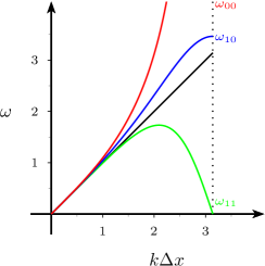
Figure 2: Dispersion relations: analytic (black) for $c=\sqrt{gH}$, ${\omega_{11}}$ in green for the Hodge-star pair $(\color[rgb]{0,0,0}\widetilde{\star}^{\,u}_{1}\color[rgb]{0,0,0},\color[rgb]{0,0,0}\widetilde{\star}^{\,h}_{1}\color[rgb]{0,0,0})$, ${\omega_{10}}$ in blue for $(\color[rgb]{0,0,0}\widetilde{\star}^{\,u}_{1}\color[rgb]{0,0,0},\color[rgb]{0,0,0}\widetilde{\star}^{\,h}_{0}\color[rgb]{0,0,0})$ or $(\color[rgb]{0,0,0}\widetilde{\star}^{\,u}_{0}\color[rgb]{0,0,0},\color[rgb]{0,0,0}\widetilde{\star}^{\,h}_{1}\color[rgb]{0,0,0}$), and ${\omega_{00}}$ in red for $(\color[rgb]{0,0,0}\widetilde{\star}^{\,u}_{0}\color[rgb]{0,0,0},\color[rgb]{0,0,0}\widetilde{\star}^{\,h}_{0}\color[rgb]{0,0,0}$).

5 Numerical analysis

The objective of this section is threefold. First, we study if the mixed and split FE discrete schemes are structure-preserving in the sense that they preserve the first principles of mass and momentum conservation. Second, we study the convergence behavior with respect to analytical solutions of the 1D wave equations. Third, we investigate if the schemes represent the corresponding discrete dispersion relations correctly.

As discussed in sections 3 and 4.4, the discrete dispersion relations differ from the analytical ones, in particular for small wave numbers. In order to avoid these error sources when investigating the convergence properties, we perform simulations with a single sine wave (corresponding to wave number $k=1$) in test case (TC) 1. Limiting the convergence tests to long waves will keep the errors introduced by the discrete dispersion relation small. This will allow us to test convergence of the schemes for integration times up to 5 cycles (which means the wave propagates 5 times through the periodic domain), despite of the influence of the wave dispersion on the shape of the wave package.

In a second test case (TC 2), we use a Gaussian distribution function with intermediate width, which consists of a superposition of all possible wave numbers. Here, the errors in the discrete dispersion relations will lead to a separation of the Gaussian wave package into its single wave components. As this effect grows in time, we will study the convergence properties of the schemes only for short integration times (less than 1 cycle).

Finally in TC 3, we use the Gaussian distribution function with very small width such that the high frequency waves have large magnitude. This allows us to study the dispersion behavior of each scheme numerically and to compare it with the analytic results of Sections 3 and 4.4.

Test cases and initialization.

For all numerical simulations, we use a uniform mesh with periodic boundaries, as shown in Fig. 1, for a domain of length $L=1000\,$m. Simulation times are measured in full periods (cycles) with time $T=\frac{L}{c}$ for 1 cycle, with respect to the wave speed $c=\sqrt{gH}$. To keep the temporal error for all mesh resolutions in the same order, we use in all simulations the same fixed time step size of $\Delta t=6.3102\cdot 10^{-04}\,$s for the high and medium accuracy, and $\Delta t=\frac{1}{200}6.3102\cdot 10^{-04}\,$s for the low accuracy schemes. These values follow from the CFL number presented in Sect. 4.3 and from the grid spacing of the highest resolved mesh applied.

We use the following analytical solutions of the 1D wave equations with $x\in[0,L]$ and $t\in\mathbbm{R}$ as initializations at time $t=0$ and to determine the convergence rates:

Analytical solution for TC 1; single sine wave:

$$\begin{split}h(x,t)&=H+\frac{\Delta H}{2}\sin\left(\frac{2\pi}{L}\big{(}x-ct\big{)}\right)+\frac{\Delta H}{2}\sin\left(\frac{2\pi}{L}\big{(}x+ct\big{)}\right),\\ u(x,t)&=\frac{c\Delta H}{2H}\sin\left(\frac{2\pi}{L}\big{(}x-ct\big{)}\right)-\frac{c\Delta H}{2H}\sin\left(\frac{2\pi}{L}\big{(}x+ct\big{)}\right),\end{split}$$ (47)

with parameters: $c=\sqrt{gH}$, $H=1000\,$m, $\Delta H=75\,$, and gravitational acceleration $g=9.81\,\rm{m}/\rm{s}^{2}$.

Analytical solution for TC 2/TC 3; Gaussian distribution with intermediate/small width:

$$\begin{split}h(x,t)&=H+\frac{\Delta H}{2}e^{-\Big{(}\frac{\Delta w}{2\pi}\sin\big{(}\frac{\pi}{L}(x-ct-x_{c})\big{)}\Big{)}^{2}}+\frac{\Delta H}{2}e^{-\Big{(}\frac{\Delta w}{2\pi}\sin\big{(}\frac{\pi}{L}(x+ct-x_{c})\big{)}\Big{)}^{2}},\\ u(x,t)&=+\frac{c\Delta H}{2H}e^{-\Big{(}\frac{\Delta w}{2\pi}\sin\big{(}\frac{\pi}{L}(x-ct-x_{c})\big{)}\Big{)}^{2}}-\frac{c\Delta H}{2H}e^{-\Big{(}\frac{\Delta w}{2\pi}\sin\big{(}\frac{\pi}{L}(x+ct-x_{c})\big{)}\Big{)}^{2}},\end{split}$$ (48)

with parameters: $\Delta w=40$, $x_{c}=\frac{1}{2}L$. For TC 3, we use the preceding analytical solution with very small width by setting $\Delta w=1000$.

A direct calculation shows that both analytical expressions are indeed solutions of the 1D wave equations (2) or (3). To initialize the discrete schemes, we project the functions $h(x,0)$ and $u(x,0)$ onto either the piecewise constant or piecewise linear FE spaces (analogously to Sect. 3 and 4).

Structure-preserving nature of the split schemes.

As shown in Sect. 4.2, the split FE schemes are structure-preserving in the sense that the corresponding discrete sets of equations preserve the splitting into topological and metric parts. Here, we illustrate that these discrete equations also fulfill the first principles of mass and momentum conservation.

In the continuous case with solutions of the wave equations for velocity $u(x,t)$ and height $h(x,t)$, we define the mass $m(t)$ of the water column and it’s momentum $p(t)$ by

$$m(t):=\int_{L}h(x,t)dx,\qquad p(t):=\int_{L}h(x,t)u(x,t)dx.$$ (49)

In fact, the first principles of mass and momentum conservation allow for the derivation of momentum and continuity equations (see e.g. [5]). Therefore, we require our structure preserving schemes to conserve these principles discretely.

In Fig. 3, we present relative errors for mass and momentum with respect to the corresponding initial values for all schemes. The results are determined using TC 2 for an integration time of $t=5T$ on a mesh with $1024$ elements for the time step sizes mentioned above. For other mesh resolutions and time step sizes, these values remain conserved at the same order of accuracy. More precisely, all schemes expose a mass conservation error (left block) at the order of $10^{-9}$ with the unstable P1–P1 FE scheme being the only exception with an error of approx. $10^{-6}$. The error in the momentum (right block) is of the order of $10^{-9}$ for all schemes.

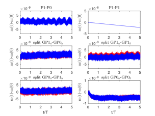
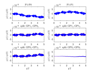
Figure 3: Conservation of mass $m(t)$ (left block) and of momentum $p(t)$ (right block) of all schemes for an integration time of $t=5T$. For the split schemes, the red lines show error values calculated with piecewise constant fields, the blue lines with piecewise linear fields.

Results for TC 1 and TC 2.

Figure 4 shows convergence towards the analytical sine wave solutions (47) for integration times $t=0.875T$ and $t=4.875T$. Similarly, in Figure 5 convergences to the analytical Gaussian-shaped solutions (48) for integration times $t=0.125T$ and $t=0.875T$ are given. To determine convergence rates valid for any smooth solution given in the form of equations (47) and (48), we use values for $t$ that are not multiples of $T/4$ such that neither height nor velocity solutions coincide with constant functions.

The reduction in integration time from about 5 cycles for TC 1 down to about 1 cycle for TC 2 is a consequence of the errors caused by the discrete dispersion relations. These lead to a deformation of the Gaussian-shaped wave package and to the development of high oscillatory waves, which prevents us from determining convergence rates in case of long integration times.

Considering the absolute error values of all split schemes for both test cases, we notice that the low accuracy ($\color[rgb]{0,0,0}{\rm GP0}_{u}\color[rgb]{0,0,0}$–$\,\color[rgb]{0,0,0}{\rm GP0}_{h}\color[rgb]{0,0,0})$ scheme has in general significantly higher error values than both medium accuracy ($\color[rgb]{0,0,0}{\rm GP1}_{u}\color[rgb]{0,0,0}$–$\,\color[rgb]{0,0,0}{\rm GP0}_{h}\color[rgb]{0,0,0}/\color[rgb]{0,0,0}{\rm GP0}_{u}\color[rgb]{0,0,0}$–$\,\color[rgb]{0,0,0}{\rm GP1}_{h}\color[rgb]{0,0,0}$) schemes, which in turn have higher error values than the high accuracy ($\color[rgb]{0,0,0}{\rm GP1}_{u}\color[rgb]{0,0,0}$–$\,\color[rgb]{0,0,0}{\rm GP1}_{h}\color[rgb]{0,0,0}$) one. This can be expected as the low accuracy scheme applies two low order closure equations, the medium schemes a combination of low and higher order, and the high accuracy scheme two higher order closure equations. Hence, these absolute error values indeed reflect how accurately the two metric closure equations are discretized.

Comparing the split with the mixed schemes, we observe a general agreement of the convergence rates of the corresponding solutions. In more detail, those fields represented by piecewise constant basis functions show the expected $1^{st}$-order convergence rate for all schemes. Moreover, the absolute error values of corresponding mixed and split schemes agree very well. As we are not aware of a mixed FE counterpart for the low accuracy case, we cannot compare it to an established FE method.

The fields represented by piecewise linear bases show the expected $2^{nd}$-order convergence rates. Here, error values calculated with the split $\color[rgb]{0,0,0}{\rm GP1}_{u}\color[rgb]{0,0,0}$–$\,\color[rgb]{0,0,0}{\rm GP1}_{h}\color[rgb]{0,0,0}$ scheme are a little smaller then those corresponding to solutions of the P1–P1 scheme, but the solutions obtained from each scheme for short and long integration times agree very well. In contrast, the $L_{2}$ error values for the $\color[rgb]{0,0,0}{\rm GP0}_{u}\color[rgb]{0,0,0}$–$\,\color[rgb]{0,0,0}{\rm GP0}_{h}\color[rgb]{0,0,0}$ scheme for the fields with piecewise linear representation increase with integration time. This property is shared by both $\color[rgb]{0,0,0}{\rm GP1}_{u}\color[rgb]{0,0,0}$–$\,\color[rgb]{0,0,0}{\rm GP0}_{h}\color[rgb]{0,0,0}$ and $\color[rgb]{0,0,0}{\rm GP0}_{u}\color[rgb]{0,0,0}$–$\,\color[rgb]{0,0,0}{\rm GP1}_{h}\color[rgb]{0,0,0}$ schemes and the mixed P1–P0 scheme, while the absolute error values of mixed and split schemes agree very well. When the $L_{2}$ errors between mixed and split schemes show small differences in low resolution meshes, they usually vanish with higher resolution.

In case of mixed P1–P1 and split $\color[rgb]{0,0,0}{\rm GP1}_{u}\color[rgb]{0,0,0}$–$\,\color[rgb]{0,0,0}{\rm GP1}_{h}\color[rgb]{0,0,0}$ schemes, we notice for high resolutions of about $2048$ and $4096$ elements with error values smaller than $10^{-4}$ a discrepancy from the $2^{nd}$-order convergence rate. At such high resolution the spatial errors are in the order of the temporal errors leading to a flattening of the convergence curve, or even to some jumps as in Fig. 4 (upper-left). This is confirmed by halving the time step size, which reduces the time step errors by a factor of $4$, which leads to the improved convergence rates as shown in (Fig. 5, upper-left)). The factor $4$ corresponds well to the expected $2^{nd}$-order convergence rate of the CN time discretization scheme, introduced in Sect. 4.3.

Both $\color[rgb]{0,0,0}{\rm GP0}_{u}\color[rgb]{0,0,0}$–$\,\color[rgb]{0,0,0}{\rm GP0}_{h}\color[rgb]{0,0,0}$ and $\color[rgb]{0,0,0}{\rm GP1}_{u}\color[rgb]{0,0,0}$–$\,\color[rgb]{0,0,0}{\rm GP0}_{h}\color[rgb]{0,0,0}/\color[rgb]{0,0,0}{\rm GP0}_{u}\color[rgb]{0,0,0}$–$\,\color[rgb]{0,0,0}{\rm GP1}_{h}\color[rgb]{0,0,0}$ schemes exhibit straight convergence lines of second order because here the temporal errors are smaller than the spatial errors. The $\color[rgb]{0,0,0}{\rm GP0}_{u}\color[rgb]{0,0,0}$–$\,\color[rgb]{0,0,0}{\rm GP0}_{h}\color[rgb]{0,0,0}$ scheme exposes spatial errors one order of magnitude larger than all other cases with resolution up to $1024$ elements, even with very small time steps (see explanation below). For the $\color[rgb]{0,0,0}{\rm GP1}_{u}\color[rgb]{0,0,0}$–$\,\color[rgb]{0,0,0}{\rm GP0}_{h}\color[rgb]{0,0,0}/\color[rgb]{0,0,0}{\rm GP0}_{u}\color[rgb]{0,0,0}$–$\,\color[rgb]{0,0,0}{\rm GP1}_{h}\color[rgb]{0,0,0}$ schemes, there is no flattening in the convergence curves as these schemes approximate the continuous dispersion relation better than the other schemes (cf. Fig. 2), which keeps the error in the time integration lower than in the unstable cases.

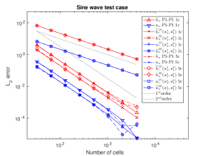
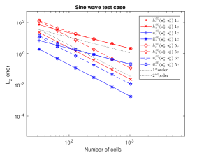
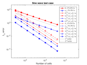
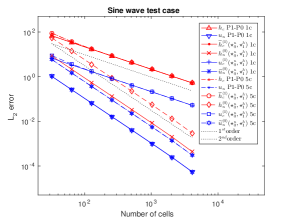
Figure 4: Convergence rates of solutions of P1–P1 and $\color[rgb]{0,0,0}{\rm GP1}_{u}\color[rgb]{0,0,0}$–$\,\color[rgb]{0,0,0}{\rm GP1}_{h}\color[rgb]{0,0,0}$ (upper left), of $\color[rgb]{0,0,0}{\rm GP0}_{u}\color[rgb]{0,0,0}$–$\,\color[rgb]{0,0,0}{\rm GP0}_{h}\color[rgb]{0,0,0}$ (upper right), of P1–P0 and $\color[rgb]{0,0,0}{\rm GP1}_{u}\color[rgb]{0,0,0}$–$\,\color[rgb]{0,0,0}{\rm GP0}_{h}\color[rgb]{0,0,0}$ (lower left), and of P1–P0 and $\color[rgb]{0,0,0}{\rm GP0}_{u}\color[rgb]{0,0,0}$–$\,\color[rgb]{0,0,0}{\rm GP1}_{h}\color[rgb]{0,0,0}$ (lower right) against analytical sine wave solution (47) for integration times $t=0.875T$ and $t=4.875T$.

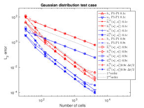
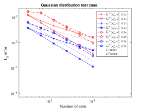
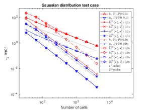
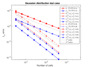
Figure 5: Convergence rates of solutions of P1–P1 and $\color[rgb]{0,0,0}{\rm GP1}_{u}\color[rgb]{0,0,0}$–$\,\color[rgb]{0,0,0}{\rm GP1}_{h}\color[rgb]{0,0,0}$ (upper left), of $\color[rgb]{0,0,0}{\rm GP0}_{u}\color[rgb]{0,0,0}$–$\,\color[rgb]{0,0,0}{\rm GP0}_{h}\color[rgb]{0,0,0}$ (upper right), of P1–P0 and $\color[rgb]{0,0,0}{\rm GP1}_{u}\color[rgb]{0,0,0}$–$\,\color[rgb]{0,0,0}{\rm GP0}_{h}\color[rgb]{0,0,0}$ (lower left), and of P1–P0 and $\color[rgb]{0,0,0}{\rm GP0}_{u}\color[rgb]{0,0,0}$–$\,\color[rgb]{0,0,0}{\rm GP1}_{h}\color[rgb]{0,0,0}$ (lower right) against analytical Gaussian wave solution (48) for integration times $t=0.125T$ and $t=0.875T$.

Results of TC 3.

Applying the Gaussian distribution (48) with very small width (TC 3), we illustrate the schemes’ representation of waves and their dispersions. To this end, we let the simulations run up to $t=0.1T$ and study how the Gaussian-shaped wave packages change their forms during simulations. These changes are a consequence of the different discrete dispersion relations for the schemes studied in this manuscript. Note that the short simulation time is justified by the design of TC 3 such that the numerical behavior in the short wave regime (right side in figure 2) is exposed.

Considering first the unstable mixed P1–P1 and split $\color[rgb]{0,0,0}{\rm GP1}_{u}\color[rgb]{0,0,0}$–$\,\color[rgb]{0,0,0}{\rm GP1}_{h}\color[rgb]{0,0,0}$ schemes in Figure 6, we notice that the piecewise linear solutions of both mixed and split schemes are very similar. At time $t=0.1T$, the left wave package travels to the left, the right one to the right. The front position on both sides agree well with the analytical solution and there are no forerunning fast waves. However, trailing oscillations develop, which change the shape of the Gaussian distribution, rendering it lower and wider. Small scale oscillations occupy the entire region between the two fronts.

As predicted by the discrete dispersion relation (44) (or by (13)), the wave with shortest wave length $k=\frac{\pi}{\Delta x}$ has zero phase velocity. This spurious mode that is not transported away from the center of the domain but oscillates on the grid scale level, is visible in Figure 6. In general, as derived theoretically, our simulations show that the phase velocity of all waves are bounded from above by $c_{d}\leq c$, and with increasing wave numbers $k$, the wave speeds get slower and slower up to the shortest wave with zero phase velocity (cf. Fig. 2).

Looking at the split $\color[rgb]{0,0,0}{\rm GP0}_{u}\color[rgb]{0,0,0}$–$\,\color[rgb]{0,0,0}{\rm GP0}_{h}\color[rgb]{0,0,0}$ scheme (cf. Figure 7), the wave packages show a similar general behavior as in the previous case. However, the differing discrete dispersion relation (46) leads to differently deformed Gaussian-shaped wave packages compared to the previous unstable schemes. As above, the peaks become smaller and wider. However, in the $\color[rgb]{0,0,0}{\rm GP0}_{u}\color[rgb]{0,0,0}$–$\,\color[rgb]{0,0,0}{\rm GP0}_{h}\color[rgb]{0,0,0}$ scheme the central part between the packages is free from high frequency modes, which indicates that the scheme does not support a standing spurious mode. On the other hand the high frequency spurious waves occur outside the central part, hence the scheme supports a fast traveling spurious mode. In fact, all waves travel with speeds equal to or larger than $c$, the analytically correct wave speed, and increase with wave number $k$ up to very large wave speeds. This is why we find waves occupying the entire outer region, and why our time step size is so much smaller when compared to the other schemes (cf. Sect. 4.4). This observation agrees very well with the discrete dispersion relation for the split $\color[rgb]{0,0,0}{\rm GP0}_{u}\color[rgb]{0,0,0}$–$\,\color[rgb]{0,0,0}{\rm GP0}_{h}\color[rgb]{0,0,0}$ scheme shown in Fig. 2.

Let us finally study simulations of TC 3 performed with the mixed P1–P0, the split $\color[rgb]{0,0,0}{\rm GP1}_{u}\color[rgb]{0,0,0}$–$\,\color[rgb]{0,0,0}{\rm GP0}_{h}\color[rgb]{0,0,0}$, and the split $\color[rgb]{0,0,0}{\rm GP0}_{u}\color[rgb]{0,0,0}$–$\,\color[rgb]{0,0,0}{\rm GP1}_{h}\color[rgb]{0,0,0}$ schemes. First of all we note that the solutions of the P1–P0 and of both split schemes agree very well. This can be inferred from Figures 8 and 9, in which the solutions of the P1–P0 scheme (green lines) and those of the split schemes (blue and red lines) show only tiny differences. Again, propagation directions are correct, while the peaks become smaller and wider. In between the peaks, no high frequency waves occupy the central region, similarly to the split $\color[rgb]{0,0,0}{\rm GP0}_{u}\color[rgb]{0,0,0}$–$\,\color[rgb]{0,0,0}{\rm GP0}_{h}\color[rgb]{0,0,0}$ scheme. In contrast to the latter however, the high frequency waves do not occupy the entire outer region but only some parts directly in front of the traveling wave packages. This reflects very well the theoretical findings described by the discrete dispersion relation (45), which states that all waves travel equal to, or faster then $c$, but not faster than about $1.1c$ (cf. Fig. 2).

\begin{overpic}[scale={0.5},unit=1mm]{13afigV1_disprel_h_GPu1GPh1zoom.pdf} \put(40.2,27.8){\includegraphics[scale={.25}]{13bfig_disprel_h_GPu1GPh1.pdf}} \end{overpic} \begin{overpic}[scale={0.5},unit=1mm]{14afigV1_disprel_u_GPu1GPh1zoom.pdf} \put(34.2,7.2){\includegraphics[scale={.27}]{14bfig_disprel_u_GPu1GPh1.pdf}} \end{overpic}

Figure 6: Illustration of the effects of the discrete dispersion relation (44) of the unstable P1–P1 and $\color[rgb]{0,0,0}{\rm GP1}_{u}\color[rgb]{0,0,0}$–$\,\color[rgb]{0,0,0}{\rm GP1}_{h}\color[rgb]{0,0,0}$ schemes on Gaussian-shaped height and velocity peaks after a simulation time of $t=0.1T$.

\begin{overpic}[scale={0.5},unit=1mm]{15afigV1_disprel_h_GPu0GPh0zoom.pdf} \put(33.0,26.2){\includegraphics[scale={.27}]{15bfig_disprel_h_GPu0GPh0.pdf}} \end{overpic} \begin{overpic}[scale={0.5},unit=1mm]{16afigV1_disprel_u_GPu0GPh0zoom.pdf} \put(9.9,6.3){\includegraphics[scale={.25}]{16bfig_disprel_u_GPu0GPh0.pdf}} \end{overpic}

Figure 7: Illustration of the effects of the discrete dispersion relation (46) of the $\color[rgb]{0,0,0}{\rm GP0}_{u}\color[rgb]{0,0,0}$–$\,\color[rgb]{0,0,0}{\rm GP0}_{h}\color[rgb]{0,0,0}$ scheme on Gaussian-shaped height and velocity peaks after a simulation time of $t=0.1T$.

\begin{overpic}[scale={0.5},unit=1mm]{17afigV1_disprel_h_GPu1GPh0zoom.pdf} \put(33.0,26.2){\includegraphics[scale={.27}]{17bfig_disprel_h_GPu1GPh0.pdf}} \end{overpic} \begin{overpic}[scale={0.5},unit=1mm]{18afigV1_disprel_u_GPu1GPh0zoom.pdf} \put(14.2,6.6){\includegraphics[scale={.27}]{18bfig_disprel_u_GPu1GPh0.pdf}} \end{overpic}

Figure 8: Illustration of the effects of the discrete dispersion relation (45) of the stable P1–P0 and $\color[rgb]{0,0,0}{\rm GP1}_{u}\color[rgb]{0,0,0}$–$\,\color[rgb]{0,0,0}{\rm GP0}_{h}\color[rgb]{0,0,0}$ schemes on Gaussian-shaped height and velocity peaks after a simulation time of $t=0.1T$.

\begin{overpic}[scale={0.5},unit=1mm]{19afigV1_disprel_h_GPu0GPh1zoom.pdf} \put(33.0,26.2){\includegraphics[scale={.27}]{19bfig_disprel_h_GPu0GPh1.pdf}} \end{overpic} \begin{overpic}[scale={0.5},unit=1mm]{20afigV1_disprel_u_GPu0GPh1zoom.pdf} \put(14.2,6.6){\includegraphics[scale={.27}]{20bfig_disprel_u_GPu0GPh1.pdf}} \end{overpic}

Figure 9: Illustration of the effects of the discrete dispersion relation (45) of the stable P1–P0 and $\color[rgb]{0,0,0}{\rm GP0}_{u}\color[rgb]{0,0,0}$–$\,\color[rgb]{0,0,0}{\rm GP1}_{h}\color[rgb]{0,0,0}$ schemes on Gaussian-shaped height and velocity peaks after a simulation time of $t=0.1T$.

6 Summary, Conclusions, Outlook

We developed a new finite element (FE) discretization framework based on the split 1D wave equations (3) with the long term objective to apply this framework to derive structure-preserving discretizations for Geophysical Fluid Dynamics (GFD) [5]. The splitting of these covariant equations into topological momentum/continuity equations and metric-dependent closure equations relies on the introduction of additional differential forms (DF). These establish pairs with the original DFs, which are connected by the Hodge-star operator. By providing proper FE spaces for all DFs such that the differential operators (here gradient and divergence) hold in strong form, our split FE framework provides discretizations that preserve geometrical structure. In particular, the discrete momentum and continuity equations are metric-free and hold in strong form (no partial integration is required). They are therefore exact up to the errors introduced by the trivial projections into the correspond FE spaces. Additional errors are however introduced by the discrete metric-dependent closure equations that provide approximations to the Hodge-star operator by nontrivial Galerkin projections (GP).

Requirements from structure preservation together with our objective to develop a lowest-order scheme for the split 1D wave equations impose certain conditions on the choice of FE spaces that approximate the corresponding DFs. In detail, both topological equations are projected onto piecewise constant spaces, whereas each of the two metric equations is projected onto both piecewise constant and piecewise linear spaces. Although this gives four possible realizations, we find in principle three classes of schemes: a high accuracy scheme ($\color[rgb]{0,0,0}{\rm GP1}\color[rgb]{0,0,0}$–$\,\color[rgb]{0,0,0}{\rm GP1}\color[rgb]{0,0,0}$), in which the Galerkin projections map onto piecewise linear (GP1) spaces, a low accuracy scheme ($\color[rgb]{0,0,0}{\rm GP0}\color[rgb]{0,0,0}$–$\,\color[rgb]{0,0,0}{\rm GP0}\color[rgb]{0,0,0}$), in which the Galerkin projections map onto piecewise constant (GP0) spaces, and two medium accuracy schemes ($\color[rgb]{0,0,0}{\rm GP1}\color[rgb]{0,0,0}$–$\,\color[rgb]{0,0,0}{\rm GP0}\color[rgb]{0,0,0}$), in which one Galerkin projection maps onto piecewise linear, the other to piecewise constant space.

A comparison to conventional methods, the unstable P1–P1 scheme that applies piecewise linear (P1) spaces to approximate both velocity and height fields, and the stable P1–P0 scheme that approximates the velocity by a piecewise linear and the height by a piecewise constant (P0) field, was performed with respect to conservation of mass and momentum, dispersion relations, and convergence behavior. Analytical derivations showed that the discrete dispersion relations of the unstable P1–P1 and $\color[rgb]{0,0,0}{\rm GP1}\color[rgb]{0,0,0}$–$\,\color[rgb]{0,0,0}{\rm GP1}\color[rgb]{0,0,0}$ schemes as well as of the stable P1–P0 and both $\color[rgb]{0,0,0}{\rm GP1}\color[rgb]{0,0,0}$–$\,\color[rgb]{0,0,0}{\rm GP0}\color[rgb]{0,0,0}$ schemes coincide, in spite of the differences in how they are derived. In particular, the $\color[rgb]{0,0,0}{\rm GP1}\color[rgb]{0,0,0}$–$\,\color[rgb]{0,0,0}{\rm GP1}\color[rgb]{0,0,0}$ scheme and the P1–P1 scheme share the problem of permitting spurious modes, whereas the stable P1–P0 scheme and the two $\color[rgb]{0,0,0}{\rm GP1}\color[rgb]{0,0,0}$–$\,\color[rgb]{0,0,0}{\rm GP0}\color[rgb]{0,0,0}$ schemes are free of such modes.

The piecewise linear fields of P1–P1 and $\color[rgb]{0,0,0}{\rm GP1}\color[rgb]{0,0,0}$–$\,\color[rgb]{0,0,0}{\rm GP1}\color[rgb]{0,0,0}$ schemes show more or less the same convergence rates of second order. Applying four instead of only two FE spaces, we illustrated that the piecewise constant fields, present only in the split schemes, showed the expected first order convergence rate. Similarly, the corresponding fields of the P1–P0 and both $\color[rgb]{0,0,0}{\rm GP1}\color[rgb]{0,0,0}$–$\,\color[rgb]{0,0,0}{\rm GP0}\color[rgb]{0,0,0}$ schemes agree in their convergence behavior. Both piecewise constant height fields show first order and both piecewise linear velocity fields second order convergence rates. Utilizing a piecewise linear approximation to the height field, the split $\color[rgb]{0,0,0}{\rm GP1}\color[rgb]{0,0,0}$–$\,\color[rgb]{0,0,0}{\rm GP0}\color[rgb]{0,0,0}$ schemes give for both velocity and height fields second order convergence rates. This combination of projections can therefore be interpreted as stable version of the conventional unstable P1–P1 scheme.

We further verified the structure-preserving nature of the split schemes fulfilling the first principles of mass and momentum conservation discretely. In more detail, the corresponding relative errors show fluctuations on the order of about $10^{-9}$ without indicating a trend. When compared to the conventional schemes, this conservation behavior is only shared by the stable P1–P0 scheme, whereas the unstable P1–P1 scheme shows a tendency to lose mass, for the given simulation time on the order of $10^{-6}$.

Besides the $\color[rgb]{0,0,0}{\rm GP1}\color[rgb]{0,0,0}$–$\,\color[rgb]{0,0,0}{\rm GP1}\color[rgb]{0,0,0}$ and $\color[rgb]{0,0,0}{\rm GP1}\color[rgb]{0,0,0}$–$\,\color[rgb]{0,0,0}{\rm GP0}\color[rgb]{0,0,0}$ schemes that have a counterpart with the P1–P1 and P1–P0 schemes in literature, we found a split $\color[rgb]{0,0,0}{\rm GP0}\color[rgb]{0,0,0}$–$\,\color[rgb]{0,0,0}{\rm GP0}\color[rgb]{0,0,0}$ scheme, for which we are not aware of a corresponding standard formulation. This low accuracy scheme preserves the first principles of mass and momentum conservation in the same way as the other split schemes. However, it does not provide a very accurate approximation to the dispersion relation, exposing very fast traveling short waves. Despite of the latter drawback, the finding of this new scheme illustrates the general character of our split FE discretization framework. By allowing a larger variety of combinations of different FE spaces compared to conventional mixed FE methods, this framework provides a toolbox to find and study new combinations of finite element spaces. In this vein, it is subject to current and future work to investigate various low- and higher-order FE space combinations to find new structure-preserving discretizations of the nonlinear rotating shallow-water equations, and of the equations of GFD in general.

7 Acknowledgements

This project has received funding from the European Union’s Horizon 2020 research and innovation programme under the Marie Skłodowska-Curie grant agreement No 657016. Additionally, the second author acknowledges support by the DFG excellence cluster CliSAP (EXC177).

Appendix A Explicit representation of mass and stiffness matrices

Here, we explicitly represent the mass and stiffness matrices used in Sect. 3 and Sect. 4. In particular, we show the coefficients which follow by evaluating the integrals of the variational formulations. Imposing periodic boundary conditions, the presented matrices correspond to a mesh with $N$ independent DoFs for nodes and elements, as illustrated in Figure 1.

The basis functions for the piecewise linear FE space are given by the Lagrange functions $\color[rgb]{0,0,0}\phi_{l}(x)\color[rgb]{0,0,0},\ \forall l=1,\dots N$, and those for the piecewise constant FE space by the step functions $\color[rgb]{0,0,0}\chi_{m}(x)\color[rgb]{0,0,0},\ \forall m=1,\dots N,$ (cf. Figure 1). They are defined by

$$\color[rgb]{0,0,0}\phi_{l}(x)\color[rgb]{0,0,0}=\begin{cases}1-\frac{x-x_{l}}{\Delta x_{m}}&\text{if}\ x\in[x_{l},x_{l+1}],\\ \frac{x-x_{l-1}}{\Delta x_{m-1}}&\text{if}\ x\in[x_{l-1},x_{l}],\\ 0&\text{else};\end{cases}\qquad\color[rgb]{0,0,0}\chi_{m}(x)\color[rgb]{0,0,0}=\begin{cases}1&\text{if}\ x\in[x_{l},x_{l+1}],\\ 0&\text{else}.\end{cases}$$ (50)

Note that, for all ${\color[rgb]{0,0,0}{l}\color[rgb]{0,0,0}}=1,\dots N$, there is $\int_{L}\color[rgb]{0,0,0}\phi_{{l-1}}(x)\color[rgb]{0,0,0}\color[rgb]{0,0,0}\phi_{l}(x)\color[rgb]{0,0,0}dx=\frac{1}{6}\Delta x_{{\color[rgb]{0,0,0}{m}\color[rgb]{0,0,0}}-1}$, $\int_{L}\color[rgb]{0,0,0}\phi_{{l}}(x)\color[rgb]{0,0,0}\color[rgb]{0,0,0}\phi_{l}(x)\color[rgb]{0,0,0}dx=\frac{1}{3}\Delta x_{{\color[rgb]{0,0,0}{m}\color[rgb]{0,0,0}}-1}+\frac{1}{3}\Delta x_{{\color[rgb]{0,0,0}{m}\color[rgb]{0,0,0}}}$, $\int_{L}\color[rgb]{0,0,0}\phi_{{l+1}}(x)\color[rgb]{0,0,0}\color[rgb]{0,0,0}\phi_{l}(x)\color[rgb]{0,0,0}dx=\frac{1}{6}\Delta x_{{\color[rgb]{0,0,0}{m}\color[rgb]{0,0,0}}}$, and zero else. Hence, the evaluation of coefficients (8) gives the metric-dependent mass-matrix

$${\bf M}^{nn}=\left(\begin{matrix}\frac{1}{3}\Delta x_{N}+\frac{1}{3}\Delta x_{1}&\frac{1}{6}\Delta x_{1}&0&\ldots&\frac{1}{6}\Delta x_{N}\\ \frac{1}{6}\Delta x_{1}&\frac{1}{3}\Delta x_{1}+\frac{1}{3}\Delta x_{2}&\frac{1}{6}\Delta x_{2}&\ldots&0\\ \vdots&\ddots&\ddots&\ddots&\vdots\\ 0&\ldots&\frac{1}{6}\Delta x_{N-2}&\frac{1}{3}\Delta x_{N-2}+\frac{1}{3}\Delta x_{N-1}&\frac{1}{6}\Delta x_{N}\\ \frac{1}{6}\Delta x_{1}&\ldots&0&\frac{1}{6}\Delta x_{N-1}&\frac{1}{3}\Delta x_{N-1}+\frac{1}{3}\Delta x_{N}\end{matrix}\right).$$ (51)

Because of the periodic boundary, we identify here and throughout the entire manuscript $\color[rgb]{0,0,0}\phi_{{0}}(x)\color[rgb]{0,0,0}$ with $\color[rgb]{0,0,0}\phi_{{N}}(x)\color[rgb]{0,0,0}$ and $\color[rgb]{0,0,0}\phi_{{N+1}}(x)\color[rgb]{0,0,0}$ with $\color[rgb]{0,0,0}\phi_{{1}}(x)\color[rgb]{0,0,0}$. Moreover, for all ${\color[rgb]{0,0,0}{l}\color[rgb]{0,0,0}}=1,\dots N$, there is $\int_{L}\frac{d\color[rgb]{0,0,0}\phi_{{l\mp 1}}(x)\color[rgb]{0,0,0}}{dx}\color[rgb]{0,0,0}\phi_{l}(x)\color[rgb]{0,0,0}dx=\mp\frac{1}{2}$, and zero else. Therefore, the evaluation of coefficients (9) gives the metric-free stiffness matrix

$${\bf D}^{nn}=\left(\begin{matrix}0&\frac{1}{2}&0&\ldots&\frac{1}{2}\\ -\frac{1}{2}&0&\frac{1}{2}&\dots&0\\ \vdots&\ddots&\ddots&\ddots&\vdots\\ 0&\ldots&-\frac{1}{2}&0&\frac{1}{2}\\ \frac{1}{2}&\ldots&0&-\frac{1}{2}&0\end{matrix}\right).$$ (52)

Applying the values $\int_{L}\color[rgb]{0,0,0}\chi_{m}(x)\color[rgb]{0,0,0}\color[rgb]{0,0,0}\chi_{m}(x)\color[rgb]{0,0,0}=\Delta x_{\color[rgb]{0,0,0}{m}\color[rgb]{0,0,0}}$ for all $m=1,\dots N$, zero else, to evaluate coefficients (18) and $\int_{L}\frac{d\color[rgb]{0,0,0}\phi_{{l/l+1}}(x)\color[rgb]{0,0,0}}{dx}\color[rgb]{0,0,0}\chi_{m}(x)\color[rgb]{0,0,0}dx=-1/1$ for all $m=1,\dots N$, zero else, to calculate coefficients (19), there follow the metric-dependent mass-matrix ${\bf M}^{ee}$ and the metric-free stiffness matrix ${\bf D}^{en}$:

$${\bf M}^{ee}=\left(\begin{matrix}\Delta x_{1}&0&\ldots&0\\ 0&\Delta x_{2}&\ldots&0\\ \vdots&\vdots&\ddots&\vdots\\ 0&0&\ldots&\Delta x_{N}\end{matrix}\right),\qquad{\bf D}^{en}=\left(\begin{matrix}-1&1&0&\ldots&0\\ 0&-1&1&\ldots&0\\ \vdots&\vdots&\ddots&\ddots&\vdots\\ 0&0&\ldots&-1&1\\ 1&0&\ldots&0&-1\end{matrix}\right),$$

with ${\bf D}^{ne}=({\bf D}^{en})^{T}$.

Finally, using the values $\int_{L}\color[rgb]{0,0,0}\chi_{{m-1/m}}(x)\color[rgb]{0,0,0}\color[rgb]{0,0,0}\phi_{l}(x)\color[rgb]{0,0,0}dx=\frac{1}{2}\Delta x_{m-1}/\frac{1}{2}\Delta x_{m}$ for all $l=1,\dots N$, zero else, the evaluation of coefficients (32) gives the metric-dependent mass-matrix ${\bf M}^{ne}$ with corresponding metric-free projection matrix ${\bf P}^{ne}$:

$${\bf M}^{ne}=\left(\begin{matrix}\frac{1}{2}\Delta x_{1}&0&\ldots&\frac{1}{2}\Delta x_{N}\vspace{0.3em}\\ \frac{1}{2}\Delta x_{1}&\frac{1}{2}\Delta x_{2}&\ldots&0\\ \vdots&\ddots&\ddots&\vdots\\ 0&\ldots&\frac{1}{2}\Delta x_{N-1}&\frac{1}{2}\Delta x_{N}\end{matrix}\right),\qquad{\bf P}^{ne}=\left(\begin{matrix}\frac{1}{2}&0&\ldots&\frac{1}{2}\vspace{0.3em}\\ \frac{1}{2}&\frac{1}{2}&\ldots&0\\ \vdots&\ddots&\ddots&\vdots\\ 0&\ldots&\frac{1}{2}&\frac{1}{2}\end{matrix}\right).$$

Appendix B Derivation of the discrete dispersion relations

In this section we present a detailed derivation of the discrete dispersion relations, presented in Sect. 3 for the mixed, and in Sect. 4 for the split schemes. For the mixed schemes we mainly follow the approach presented in [23]. For the split schemes, we adapt this approach such that it suits to the split form of the wave equations.

B.1 The analytical case

To explain the method, we first determine the dispersion relation for the analytical wave equations. As above, we consider the domain $L$ with coordinates $x\in[0,L]\subset\mathbbm{R}$ and time variable $t\in\mathbbm{R}$. We assume that the solutions can be formulated as periodic in space and time. In more detail, we seek periodic solutions of the equations (2), i.e. we decompose the solutions like

$$u(x,t)=\hat{u}(x)e^{i\omega t}=\overline{u}e^{i\omega t-ikx},\quad h(x,t)=\hat{h}(x)e^{i\omega t}=\overline{h}e^{i\omega t-ikx},$$ (53)

in which $\overline{u},\overline{h}$ are constants. $\omega$ is the angular frequency and $k$ is the wave number.

Applying the first decomposition of (53) with respect to time to evaluate the time derivative of (2), we obtain equations in harmonic form

$$i\omega\hat{u}(x)+g\frac{\partial\hat{h}(x)}{\partial x}=0,\quad i\omega\hat{h}(x)+H\frac{\partial\hat{u}(x)}{\partial x}=0\,.$$ (54)

Using further the second decomposition of (53) in wave vector space with wave vector $k$, we find

$$\left(\begin{array}[]{cc}i\omega&igk\\ iHk&i\omega\end{array}\right)\left(\begin{array}[]{c}\overline{u}\\ \overline{h}\end{array}\right)=0\,.$$ (55)

For nontrivial solutions to exist, the determinant of the coefficient matrix in (55) must vanish. Then, the analytic dispersion relation for shallow-water waves reads

$$c=\frac{\omega}{k}=\pm\sqrt{gH}\,,$$ (56)

in which $c$ describes the phase velocity. The positive and negative solutions stand for right and left traveling waves, respectively.

The preceding equation also describes the analytical dispersion relation of the split wave equations (3). This fact follows directly by substituting in (3) the metric into the topological equations, which leads to equations (2). An explicit treatment of the split equations avoiding such substitution, as presented in Sect. B.2.3 for the discrete case, would result in the dispersion relation (56) too.

B.2 The discrete case

The discrete dispersion relations of the schemes derived in this manuscript can be calculated analogously to the continuous case. In particular, we begin our derivations from equations in harmonic form (as in (54)), in which the equations are continuous in time and only discretized in space. Representing the variables in terms of Fourier expansions on nodal and elemental unknowns, this approach results in discrete dispersion relations in which the magnitude of the temporal frequency is expressed as a function of the wave number $k$, cf. [16, 17].

To simplify calculations, we assume for all the following cases that the domain with length $L$ is discretized by a uniform mesh whose $N$ elements have equilateral size $\Delta x=\Delta x_{m}=x_{l+1}-x_{l}=\frac{L}{N}$ for all $m,l=1,\dots N$, (cf. Fig. 1).

B.2.1 The unstable P1–P1 FE scheme

The semi-discrete harmonic equations of the unstable P1–P1 scheme are given by (6) in Sect. 3.1, in which the partial time derivatives $\partial_{t}\color[rgb]{0,0,0}u_{l}\color[rgb]{0,0,0}(t)$ and $\partial_{t}\color[rgb]{0,0,0}h_{l}\color[rgb]{0,0,0}(t)$ are replaced by $i\omega\color[rgb]{0,0,0}u_{l}\color[rgb]{0,0,0}$ and $i\omega\color[rgb]{0,0,0}h_{l}\color[rgb]{0,0,0}$, respectively. Expanding further all nodal values $\color[rgb]{0,0,0}u_{l}\color[rgb]{0,0,0},\color[rgb]{0,0,0}h_{l}\color[rgb]{0,0,0}$ in wave vector form, i.e. $\color[rgb]{0,0,0}u_{l}\color[rgb]{0,0,0}=\overline{u}e^{ikx_{l}},\color[rgb]{0,0,0}h_{l}\color[rgb]{0,0,0}=\overline{h}e^{ikx_{l}}$ for constants $\overline{u}$ and $\overline{h}$, we obtain

$$\begin{split}&i\omega\left\{\begin{array}[]{c}\overline{u}\\ \overline{h}\end{array}\right\}\Big{(}e^{ikx_{l-1}}\int_{L}\color[rgb]{0,0,0}\phi_{{l-1}}(x)\color[rgb]{0,0,0}\color[rgb]{0,0,0}\phi_{l}(x)\color[rgb]{0,0,0}dx+e^{ikx_{l}}\int_{L}\color[rgb]{0,0,0}\phi_{{l}}(x)\color[rgb]{0,0,0}\color[rgb]{0,0,0}\phi_{l}(x)\color[rgb]{0,0,0}dx+e^{ikx_{l+1}}\int_{L}\color[rgb]{0,0,0}\phi_{{l+1}}(x)\color[rgb]{0,0,0}\color[rgb]{0,0,0}\phi_{l}(x)\color[rgb]{0,0,0}dx\Big{)}\\ &+\left\{\begin{array}[]{c}g\\ H\end{array}\right\}\left\{\begin{array}[]{c}\overline{h}\\ \overline{u}\end{array}\right\}\Big{(}e^{ikx_{l-1}}\int_{L}\frac{d\color[rgb]{0,0,0}\phi_{{l-1}}(x)\color[rgb]{0,0,0}}{dx}\color[rgb]{0,0,0}\phi_{l}(x)\color[rgb]{0,0,0}dx+e^{ikx_{l+1}}\int_{L}\frac{d\color[rgb]{0,0,0}\phi_{{l+1}}(x)\color[rgb]{0,0,0}}{dx}\color[rgb]{0,0,0}\phi_{l}(x)\color[rgb]{0,0,0}dx\Big{)}=0\ \forall{\color[rgb]{0,0,0}{l}\color[rgb]{0,0,0}}=1,\dots N.\end{split}$$ (57)

Dividing the preceding equations by $e^{ikx_{l}}$ and noting that $\Delta x:=x_{l+1}-x_{l}=x_{l}-x_{l-1}$, we find

$$\begin{split}&i\omega\left\{\begin{array}[]{c}\overline{u}\\ \overline{h}\end{array}\right\}\Delta x\Big{(}\frac{2}{3}+\frac{1}{6}e^{-ik\Delta x}+\frac{1}{6}e^{ik\Delta x}\Big{)}+\left\{\begin{array}[]{c}g\\ H\end{array}\right\}\left\{\begin{array}[]{c}\overline{h}\\ \overline{u}\end{array}\right\}\Big{(}-\frac{1}{2}e^{-ik\Delta x}+\frac{1}{2}e^{ik\Delta x}\Big{)}=0\,,\\ &i\omega\left\{\begin{array}[]{c}\overline{u}\\ \overline{h}\end{array}\right\}\Delta x\Big{(}\frac{2}{3}+\frac{1}{3}\cos(k\Delta x)\Big{)}+\left\{\begin{array}[]{c}g\\ H\end{array}\right\}\left\{\begin{array}[]{c}\overline{h}\\ \overline{u}\end{array}\right\}\Big{(}i\sin(k\Delta x)\Big{)}=0,\end{split}$$ (58)

where we used the integral values of Appendix A. Equivalently, these equations can be written in matrix-vector form:

$$\left(\begin{array}[]{cc}\frac{i\omega}{3}\Big{(}2+\cos(k\Delta x)\Big{)}&\frac{ig}{\Delta x}\sin(k\Delta x)\\ \frac{iH}{\Delta x}\sin(k\Delta x)&\frac{i\omega}{3}\Big{(}2+\cos(k\Delta x)\Big{)}\end{array}\right)\left(\begin{array}[]{c}\overline{u}\\ \overline{h}\end{array}\right)=0.$$ (59)

Setting the determinant of this coefficient matrix to zero gives the discrete dispersion relation

$$c_{d}=\frac{\omega}{k}=\pm\sqrt{gH}\frac{\sin(k\Delta x)}{k\Delta x}\frac{3}{2+\cos(k\Delta x)}\,.$$ (60)

For $k\rightarrow 0$, there follows $c_{d}\rightarrow c=\sqrt{gH}$, which can be verified by expanding $\sin(k{\Delta x})$ in a Taylor series around zero. At the shortest wave length $k=\frac{\pi}{\Delta x}$, equation (60) has a second root (spurious mode). Therefore, the P1–P1 scheme is unstable.

B.2.2 The stable P1–P0 FE scheme

In case of the stable P1–P0 scheme introduced in Sect. 3.2, the semi-discrete harmonic equations are given by (16), with $\partial_{t}\color[rgb]{0,0,0}u_{l}\color[rgb]{0,0,0}(t)$ and $\partial_{t}\color[rgb]{0,0,0}h_{m}\color[rgb]{0,0,0}(t)$ replaced by $i\omega\color[rgb]{0,0,0}u_{l}\color[rgb]{0,0,0}$ and $i\omega\color[rgb]{0,0,0}h_{m}\color[rgb]{0,0,0}$, respectively. Here we expand the variables for all nodes as $\color[rgb]{0,0,0}u_{l}\color[rgb]{0,0,0}=\overline{u}e^{ikx_{l}}$ and for all elements as $\color[rgb]{0,0,0}h_{m}\color[rgb]{0,0,0}=\overline{h}e^{ikx_{m}}$.

Then, the discrete momentum equation reads

$$\begin{split}&i\omega\overline{u}\Big{(}e^{ikx_{l-1}}\int_{L}\color[rgb]{0,0,0}\phi_{{l-1}}(x)\color[rgb]{0,0,0}\color[rgb]{0,0,0}\phi_{l}(x)\color[rgb]{0,0,0}dx+e^{ikx_{l}}\int_{L}\color[rgb]{0,0,0}\phi_{l}(x)\color[rgb]{0,0,0}\color[rgb]{0,0,0}\phi_{l}(x)\color[rgb]{0,0,0}dx+e^{ikx_{l+1}}\int_{L}\color[rgb]{0,0,0}\phi_{{l+1}}(x)\color[rgb]{0,0,0}\color[rgb]{0,0,0}\phi_{l}(x)\color[rgb]{0,0,0}dx\Big{)}\\ &-g\overline{h}\Big{(}e^{ikx_{m-1}}\int_{L}\color[rgb]{0,0,0}\chi_{{m-1}}(x)\color[rgb]{0,0,0}\frac{d\color[rgb]{0,0,0}\phi_{l}(x)\color[rgb]{0,0,0}}{dx}dx+e^{ikx_{m}}\int_{L}\color[rgb]{0,0,0}\chi_{{m}}(x)\color[rgb]{0,0,0}\frac{d\color[rgb]{0,0,0}\phi_{l}(x)\color[rgb]{0,0,0}}{dx}dx\Big{)}=0,\ \forall\ l=1,\dots N,\end{split}$$ (61)

and the continuity equation reads

$$\begin{split}&i\omega\overline{h}e^{ikx_{m}}\int_{L}\color[rgb]{0,0,0}\chi_{m}(x)\color[rgb]{0,0,0}\color[rgb]{0,0,0}\chi_{m}(x)\color[rgb]{0,0,0}dx+\\ &H\overline{u}\Big{(}e^{ikx_{l}}\int_{L}\frac{d\color[rgb]{0,0,0}\phi_{{l}}(x)\color[rgb]{0,0,0}}{dx}\color[rgb]{0,0,0}\chi_{m}(x)\color[rgb]{0,0,0}dx+e^{ikx_{l+1}}\int_{L}\frac{d\color[rgb]{0,0,0}\phi_{{l+1}}(x)\color[rgb]{0,0,0}}{dx}\color[rgb]{0,0,0}\chi_{m}(x)\color[rgb]{0,0,0}dx\Big{)}=0,\ \forall\ m=1,\dots N.\end{split}$$ (62)

Dividing the former equation by $e^{ikx_{l}}$ and the latter by $e^{ikx_{m}}$, noting that $\frac{\Delta x}{2}=x_{l+1}-x_{m}=x_{m}-x_{l-1}$ on a uniform mesh, and using the integral values of Appendix A, the momentum equation becomes

$$\begin{split}i\omega\overline{u}\Delta x\Big{(}\frac{2}{3}+\frac{1}{6}e^{-ik\Delta x}+\frac{1}{6}e^{ik\Delta x}\Big{)}+g\overline{h}\Big{(}-e^{-ik\frac{\Delta x}{2}}+e^{ik\frac{\Delta x}{2}}\Big{)}&=0\,,\\ i\omega\overline{u}\Delta x\Big{(}\frac{2}{3}+\frac{1}{3}\cos(k\Delta x)\Big{)}+g\overline{h}2i\sin\left(k\frac{\Delta x}{2}\right)&=0\,,\end{split}$$ (63)

and the continuity equation becomes

$$\begin{split}i\omega\overline{h}\Delta x+H\overline{u}\Big{(}-e^{-ik\frac{\Delta x}{2}}+e^{ik\frac{\Delta x}{2}}\Big{)}&=0\,,\\ i\omega\overline{h}\Delta x+H\overline{u}2i\sin\left(k\frac{\Delta x}{2}\right)&=0\,.\\ \end{split}$$ (64)

In matrix-vector formulation, the preceding set of discrete equations yields

$$\left(\begin{array}[]{cc}\frac{i\omega}{3}\left(2+\cos(k\Delta x)\right)&\frac{i2g}{\Delta x}\sin(k\frac{\Delta x}{2})\vspace{0.3em}\\ \frac{i2H}{\Delta x}\sin(k\frac{\Delta x}{2})&i\omega\end{array}\right)\left(\begin{array}[]{c}\overline{u}\vspace{0.3em}\\ \overline{h}\end{array}\right)=0\,.$$ (65)

Setting the determinant of this coefficient matrix to zero results in the discrete dispersion relation

$$c_{d}=\frac{\omega}{k}=\pm\sqrt{gH}\frac{\sin(k\frac{\Delta x}{2})}{k\frac{\Delta x}{2}}\left[\frac{3}{2+\cos(k\Delta x)}\right]^{1/2}\,.$$ (66)

Also here, $c_{d}\rightarrow c$ for $k\rightarrow 0$. However, in contrast to the unstable P1–P1 scheme, there is no second root at shortest wave length $k=\frac{\pi}{\Delta x}$. Instead, the discrete dispersion relation approximates well the analytical one. Therefore, we consider this scheme as stable.

B.2.3 The split FE schemes

For the split schemes derived in Sect. 4, the semi-discrete harmonic topological equations are given by (29), with $\partial_{t}\color[rgb]{0,0,0}u_{m}\color[rgb]{0,0,0}(t)$ and $\partial_{t}\color[rgb]{0,0,0}\widetilde{h}_{m}\color[rgb]{0,0,0}(t)$ replaced by $i\omega\color[rgb]{0,0,0}u_{m}\color[rgb]{0,0,0}$ and $i\omega\color[rgb]{0,0,0}\widetilde{h}_{m}\color[rgb]{0,0,0}$, respectively. Here we expand the coefficient of velocity and height in wave vector form as follows: at nodal values as $\color[rgb]{0,0,0}\widetilde{u}_{l}\color[rgb]{0,0,0}=\overline{\widetilde{u}}e^{ikx_{l}},\color[rgb]{0,0,0}h_{l}\color[rgb]{0,0,0}=\overline{h}e^{ikx_{l}}$, and at elemental values as $\color[rgb]{0,0,0}\widetilde{h}_{m}\color[rgb]{0,0,0}=\overline{\widetilde{h}}e^{ikx_{m}},\color[rgb]{0,0,0}u_{m}\color[rgb]{0,0,0}=\overline{u}e^{ikx_{m}}$, with constants $\overline{\widetilde{u}},\overline{h},\overline{\widetilde{h}},$ and $\overline{u}$. We obtain

$$\begin{split}&i\omega\left\{\begin{array}[]{c}\overline{u}\\ \overline{\widetilde{h}}\end{array}\right\}\Big{(}e^{ikx_{m}}\int_{L}\color[rgb]{0,0,0}\chi_{m}(x)\color[rgb]{0,0,0}\color[rgb]{0,0,0}\chi_{m}(x)\color[rgb]{0,0,0}dx\Big{)}\\ &+\left\{\begin{array}[]{c}g\\ H\end{array}\right\}\left\{\begin{array}[]{c}\overline{h}\\ \overline{\widetilde{u}}\end{array}\right\}\Big{(}e^{ikx_{l}}\int_{L}\frac{d\color[rgb]{0,0,0}\phi_{{l}}(x)\color[rgb]{0,0,0}}{dx}\color[rgb]{0,0,0}\chi_{m}(x)\color[rgb]{0,0,0}dx+e^{ikx_{l+1}}\int_{L}\frac{d\color[rgb]{0,0,0}\phi_{{l+1}}(x)\color[rgb]{0,0,0}}{dx}\color[rgb]{0,0,0}\chi_{m}(x)\color[rgb]{0,0,0}dx\Big{)}=0,\ \forall{\color[rgb]{0,0,0}{m}\color[rgb]{0,0,0}}=1,\dots N.\end{split}$$ (67)

Dividing the preceding equations by $e^{ikx_{m}}$ and using $\frac{\Delta x}{2}=x_{l+1}-x_{m}=x_{m}-x_{l-1}$ and the integral values of Appendix A, there follows

$$\begin{split}i\omega\left\{\begin{array}[]{c}\overline{u}\\ \overline{\widetilde{h}}\end{array}\right\}\Delta x+\left\{\begin{array}[]{c}g\\ H\end{array}\right\}\left\{\begin{array}[]{c}\overline{h}\\ \overline{\widetilde{u}}\end{array}\right\}\Big{(}e^{ik\frac{\Delta x}{2}}-e^{-ik\frac{\Delta x}{2}}\Big{)}&=0\,,\\ i\omega\left\{\begin{array}[]{c}\overline{u}\\ \overline{\widetilde{h}}\end{array}\right\}+\left\{\begin{array}[]{c}g\\ H\end{array}\right\}\left\{\begin{array}[]{c}\overline{h}\\ \overline{\widetilde{u}}\end{array}\right\}\frac{2i}{\Delta x}\sin\left(k\frac{\Delta x}{2}\right)&=0\,.\\ \end{split}$$ (68)

In Sect. 4.2.2, we presented four realizations of discrete metric equations as closure conditions to the topological equations (30). Here we proceed similarly and derive discrete metric equations that close the harmonic equations (68), i.e. we distinguish between high, medium, and low accuracy closures.

High accuracy closure.

The discrete metric closure equations for the high accuracy case are given by (31). Representing the variables in wave vector form at nodal and elemental values using the expansion as for the topological equations, we obtain

$$\begin{split}&\left\{\begin{array}[]{c}\overline{\widetilde{u}}\\ \overline{h}\end{array}\right\}\Big{(}e^{ikx_{l-1}}\int_{L}\color[rgb]{0,0,0}\phi_{{l-1}}(x)\color[rgb]{0,0,0}\color[rgb]{0,0,0}\phi_{l}(x)\color[rgb]{0,0,0}dx+e^{ikx_{l}}\int_{L}\color[rgb]{0,0,0}\phi_{{l}}(x)\color[rgb]{0,0,0}\color[rgb]{0,0,0}\phi_{l}(x)\color[rgb]{0,0,0}dx+e^{ikx_{l+1}}\int_{L}\color[rgb]{0,0,0}\phi_{{l+1}}(x)\color[rgb]{0,0,0}\color[rgb]{0,0,0}\phi_{l}(x)\color[rgb]{0,0,0}dx\Big{)}\\ &=\left\{\begin{array}[]{c}\overline{u}\\ \overline{\widetilde{h}}\end{array}\right\}\Big{(}e^{ikx_{m-1}}\int_{L}\color[rgb]{0,0,0}\chi_{{m-1}}(x)\color[rgb]{0,0,0}\color[rgb]{0,0,0}\phi_{l}(x)\color[rgb]{0,0,0}dx+e^{ikx_{m}}\int_{L}\color[rgb]{0,0,0}\chi_{{m}}(x)\color[rgb]{0,0,0}\color[rgb]{0,0,0}\phi_{l}(x)\color[rgb]{0,0,0}dx\Big{)}\ \forall{\color[rgb]{0,0,0}{l}\color[rgb]{0,0,0}}=1,\dots N.\end{split}$$ (69)

Dividing the preceding equation by $e^{ikx_{l}}$, using $\frac{\Delta x}{2}=x_{l+1}-x_{m}=x_{m}-x_{l-1}$, and applying the integral values of Appendix A, we find

$$\begin{split}\left\{\begin{array}[]{c}\overline{\widetilde{u}}\\ \overline{h}\end{array}\right\}\Delta x\Big{(}\frac{2}{3}+\frac{1}{6}e^{-ik\Delta x}+\frac{1}{6}e^{ik\Delta x}\Big{)}&=\left\{\begin{array}[]{c}\overline{u}\\ \overline{\widetilde{h}}\end{array}\right\}\frac{\Delta x}{2}\Big{(}e^{-ik\frac{\Delta x}{2}}+e^{ik\frac{\Delta x}{2}}\Big{)}\,,\\ \left\{\begin{array}[]{c}\overline{\widetilde{u}}\\ \overline{h}\end{array}\right\}\Big{(}\frac{2}{3}+\frac{1}{3}\cos(k\Delta x)\Big{)}&=\left\{\begin{array}[]{c}\overline{u}\\ \overline{\widetilde{h}}\end{array}\right\}\cos\left(k\frac{\Delta x}{2}\right).\end{split}$$ (70)

The combination of these latter with the discrete topological equations (68) gives the matrix-vector equations:

$$\left(\begin{array}[]{cccc}i\omega&i\frac{2g}{\Delta x}\sin(k\frac{\Delta x}{2})&0&0\\ 0&0&i\frac{2H}{\Delta x}\sin(k\frac{\Delta x}{2})&i\omega\\ -\cos(k\frac{\Delta x}{2})&0&\Big{(}\frac{2}{3}+\frac{1}{3}\cos(k\Delta x)\Big{)}&0\\ 0&\Big{(}\frac{2}{3}+\frac{1}{3}\cos(k\Delta x)\Big{)}&0&-\cos(k\frac{\Delta x}{2})\end{array}\right)\left(\begin{array}[]{c}\overline{u}\vspace{0.4ex}\\ \overline{h}\vspace{0.4ex}\\ \overline{\widetilde{u}}\vspace{0.4ex}\\ \overline{\widetilde{h}}\\ \end{array}\right)=0\,.$$ (71)

To find nontrivial solutions of this equation, we set the determinant of this coefficient matrix to zero. There follows the discrete dispersion relation

$$c_{d}=\frac{{\omega_{11}}}{k}=\pm\sqrt{gH}\frac{\sin(k\frac{\Delta x}{2})}{k\frac{\Delta x}{2}}\frac{3\cos(k\frac{\Delta x}{2})}{(2+\cos(k\Delta x))}\,.$$ (72)

For $k\rightarrow 0$, there follows $c_{d}\rightarrow c$. The high accuracy scheme $\color[rgb]{0,0,0}{\rm GP1}_{u}\color[rgb]{0,0,0}$–$\,\color[rgb]{0,0,0}{\rm GP1}_{h}\color[rgb]{0,0,0}$ has a root solution at $k=\frac{\pi}{\Delta x}$ and is hence unstable. Because of the double angle formula (i.e. $\sin(k\Delta x)=2\sin(k\frac{\Delta x}{2})\cos(k\frac{\Delta x}{2})$), this dispersion relation equals the one in (60) for the unstable P1–P1 scheme.

Low accuracy closure.

In the low accuracy case, the discrete metric equations are given by (34), in which the variables at nodal and elemental values are expanded as for the topological equations. Then,

$$\begin{split}&\left\{\begin{array}[]{c}\overline{\widetilde{u}}\\ \overline{h}\end{array}\right\}\Big{(}e^{ikx_{l}}\int_{L}\color[rgb]{0,0,0}\phi_{{l}}(x)\color[rgb]{0,0,0}\color[rgb]{0,0,0}\chi_{m}(x)\color[rgb]{0,0,0}dx+e^{ikx_{l+1}}\int_{L}\color[rgb]{0,0,0}\phi_{{l+1}}(x)\color[rgb]{0,0,0}\color[rgb]{0,0,0}\chi_{m}(x)\color[rgb]{0,0,0}dx\Big{)}\\ &=\left\{\begin{array}[]{c}\overline{u}\\ \overline{\widetilde{h}}\end{array}\right\}e^{ikx_{m}}\int_{L}\color[rgb]{0,0,0}\chi_{m}(x)\color[rgb]{0,0,0}\color[rgb]{0,0,0}\chi_{m}(x)\color[rgb]{0,0,0}dx,\ \forall{\color[rgb]{0,0,0}{m}\color[rgb]{0,0,0}}=1,\dots N.\end{split}$$ (73)

Dividing the latter equations by $e^{ikx_{m}}$, applying $\frac{\Delta x}{2}=x_{l+1}-x_{m}=x_{m}-x_{l-1}$, and using the integral values of Appendix A, there follows

$$\begin{split}\left\{\begin{array}[]{c}\overline{\widetilde{u}}\\ \overline{h}\end{array}\right\}\frac{\Delta x}{2}\Big{(}e^{-ik\frac{\Delta x}{2}}+e^{ik\frac{\Delta x}{2}}\Big{)}&=\left\{\begin{array}[]{c}\overline{u}\\ \overline{\widetilde{h}}\end{array}\right\}\,,\\ \left\{\begin{array}[]{c}\overline{\widetilde{u}}\\ \overline{h}\end{array}\right\}\cos\left(k\frac{\Delta x}{2}\right)&=\left\{\begin{array}[]{c}\overline{u}\\ \overline{\widetilde{h}}\end{array}\right\}\,.\end{split}$$ (74)

Combining the preceding equations with (68) gives the matrix-vector equations

$$\left(\begin{array}[]{cccc}i\omega&i\frac{2g}{\Delta x}\sin(k\frac{\Delta x}{2})&0&0\\ 0&0&i\frac{2H}{\Delta x}\sin(k\frac{\Delta x}{2})&i\omega\\ 1&0&-\cos(k\frac{\Delta x}{2})&0\\ 0&-\cos(k\frac{\Delta x}{2})&0&1\end{array}\right)\left(\begin{array}[]{c}\overline{u}\vspace{0.4ex}\\ \overline{h}\vspace{0.4ex}\\ \overline{\widetilde{u}}\vspace{0.4ex}\\ \overline{\widetilde{h}}\\ \end{array}\right)=0\,.$$ (75)

To find nontrivial solutions of this system, we set the determinant of this coefficient matrix to zero. This gives the discrete dispersion relation

$$c_{d}=\frac{{\omega_{00}}}{k}=\pm\sqrt{gH}\frac{\tan(k\frac{\Delta x}{2})}{k\frac{\Delta x}{2}},$$ (76)

where $c_{d}\rightarrow c$ for $k\rightarrow 0$. At wave number $k=\frac{\pi}{\Delta x}$, there is no second root but a singularity. That is, with increasing wave number $k\rightarrow\frac{\pi}{\Delta x}$, the phase velocity tends to infinity. Therefore, we consider the low accuracy scheme $\color[rgb]{0,0,0}{\rm GP0}_{u}\color[rgb]{0,0,0}$–$\,\color[rgb]{0,0,0}{\rm GP0}_{h}\color[rgb]{0,0,0}$ as unstable.

Medium accuracy closure.

Similarly to Sect. 4.2.2, we discuss two medium accuracy closures. For the $\color[rgb]{0,0,0}{\rm GP1}_{u}\color[rgb]{0,0,0}$–$\,\color[rgb]{0,0,0}{\rm GP0}_{h}\color[rgb]{0,0,0}$ scheme corresponding to the discrete Hodge-star pair $(\color[rgb]{0,0,0}\widetilde{\star}^{\,u}_{1}\color[rgb]{0,0,0},\color[rgb]{0,0,0}\widetilde{\star}^{\,h}_{0}\color[rgb]{0,0,0})$, the discrete metric equations are given by (36). Using the expansions of the variables as above, the resulting closure equation for the velocities is given by (69), and for the height fields by (73). Combining the latter with the topological equations (68), we obtain the matrix-vector equations

$$\left(\begin{array}[]{cccc}i\omega&i\frac{2g}{\Delta x}\sin(k\frac{\Delta x}{2})&0&0\\ 0&0&i\frac{2H}{\Delta x}\sin(k\frac{\Delta x}{2})&i\omega\\ -\cos(k\frac{\Delta x}{2})&0&\Big{(}\frac{2}{3}+\frac{1}{3}\cos(k\Delta x)\Big{)}&0\\ 0&-\cos(k\frac{\Delta x}{2})&0&1\end{array}\right)\left(\begin{array}[]{c}\overline{u}\vspace{0.4ex}\\ \overline{h}\vspace{0.4ex}\\ \overline{\widetilde{u}}\vspace{0.4ex}\\ \overline{\widetilde{h}}\\ \end{array}\right)=0\,.$$ (77)

For the $\color[rgb]{0,0,0}{\rm GP0}_{u}\color[rgb]{0,0,0}$–$\,\color[rgb]{0,0,0}{\rm GP1}_{h}\color[rgb]{0,0,0}$ scheme corresponding to the discrete Hodge-star pair $(\color[rgb]{0,0,0}\widetilde{\star}^{\,u}_{0}\color[rgb]{0,0,0},\color[rgb]{0,0,0}\widetilde{\star}^{\,h}_{1}\color[rgb]{0,0,0})$, the discrete metric equations are given by (38). Expanding the variables as above, the resulting closure equation for the velocities is now given by (73) and for the height fields by (69). The combination of the latter with the discrete topological equations yields

$$\left(\begin{array}[]{cccc}i\omega&i\frac{2g}{\Delta x}\sin(k\frac{\Delta x}{2})&0&0\\ 0&0&i\frac{2H}{\Delta x}\sin(k\frac{\Delta x}{2})&i\omega\\ 1&0&-\cos(k\frac{\Delta x}{2})&0\\ 0&\Big{(}\frac{2}{3}+\frac{1}{3}\cos(k\Delta x)\Big{)}&0&-\cos(k\frac{\Delta x}{2})\end{array}\right)\left(\begin{array}[]{c}\overline{u}\vspace{0.4ex}\\ \overline{h}\vspace{0.4ex}\\ \overline{\widetilde{u}}\vspace{0.4ex}\\ \overline{\widetilde{h}}\\ \end{array}\right)=0\,.$$ (78)

Setting the determinants of these coefficient matrices to zero, there follows for both cases the same discrete dispersion relation

$$c_{d}=\frac{{\omega_{10}}}{k}=\pm\sqrt{gH}\frac{\sin(k\frac{\Delta x}{2})}{k\frac{\Delta x}{2}}\left[\frac{3}{(2+\cos(k\Delta x))}\right]^{\frac{1}{2}},$$ (79)

with $c_{d}\rightarrow c$ for $k\rightarrow 0$. For the wave number $k=\frac{\pi}{\Delta x}$, there is neither a second root nor a singularity. The dispersion relation (79) equals exactly the one in (66) of the stable P1–P0 scheme. Hence, we consider both medium accuracy schemes as stable.

Remark.

Considering the matrix-vector equations for all four cases, we realize that the first two lines remain unchanged while the second two lines change with the choice of discrete metric equations. Incorporating how the straight and twisted forms are connected, it is the choice of the metric equations that determine – by these last two lines – the schemes’ discrete dispersion relations.

References

• [1] Arnold, D. N. [2002], Differential complexes and numerical stability. Proceedings of the International Congress of Mathematicians, Beijing, 1, 137–157.
• [2] Arnold, D. N., Falk, R. S., and Winther, R. [2006], Finite element exterior calculus, homological techniques, and applications. Acta Numerica, 15, 1–155.
• [3] Arnold, D. N., Falk, R. S., and Winther, R. [2010], Finite element exterior calculus: from Hodge theory to numerical stability. Bull. Amer. Math. Soc. (N.S.), 47, 281–354.
• [4] Bauer, W. [2013], Toward Goal-Oriented R-adaptive Models in Geophysical Fluid Dynamics using a Generalized Discretization Approach. PhD thesis, Department of Geosciences, University of Hamburg.
• [5] Bauer, W. [2016], A new hierarchically-structured n-dimensional covariant form of rotating equations of geophysical fluid dynamics, GEM - International Journal on Geomathematics, 7(1), 31–101.
• [6] Behrens, J. [2006], Adaptive Atmospheric Modeling - Key Techniques in Grid Generation, Data Structures, and Numerical Operations with Applications. Lecture Notes in Computational Science and Engineering, 54, Springer Verlag, Berlin, Heidelberg, doi:10.1007/3-540-33383-5.
• [7] Bochev, P. and Hyman, J. [2006], Principles of mimetic discretizations of differential operators. Compatible Spatial Discretizations, The IMA Volumes in Mathematics and its Applications, 142, 89–119.
• [8] Boffi, Daniele and Fortin, Michel and Brezzi, Franco [2013], Mixed finite element methods and applications, Springer series in computational mathematics, Springer, Berlin, Heidelberg.
• [9] Bossavit, A. [2001], ’Generalized finite differences’ in computational electromagnetics, Progress In Electromagnetics Research (PIER), 32, 45–64.
• [10] Cotter, C.J. and Ham, D.A. and Pain, C.C. and Reich, S. [2009], LBB stability of a mixed Galerkin finite element pair for fluid flow simulations, Journal of Computational Physics.
• [11] Cotter, C.J. and McRae, A.T.T. [2014], Compatible finite elements for numerical weather prediction, arXiv:1401.0616, https://arxiv.org/abs/1401.0616.
• [12] Cotter, C.J., Thuburn, J. [2012], A finite element exterior calculus framework for the rotating shallow-water equations, Journal of Computational Physics, 257(B), 1506–1526.
• [13] Desbrun, M., Hirani, A. N., Leok, M., and Marsden, J. E. [2005], Discrete exterior calculus, arXiv:math/0508341v2 [math.DG].
• [14] Kreeft, J. J. and Palha, A. and Gerritsma, M. I. [2010], Mimetic spectral element method for generalized convection-diffusion problems. In Proceedings of the European Conference on Computational Fluid Dynamics (ECCOMAS CFD).
• [15] Lee, J. J., and Winther, R. [2016], Local coderivatives and approximation of Hodge Laplace problems, To appear. arXiv preprint 1610.07954, https://arxiv.org/abs/1610.07954.
• [16] Le Roux, D. Y. and Rostand, V. and Benoit, P. [2007], Analysis of Numerically Induced Oscillations in 2D Finite-Element Shallow-Water Models Part I: Inertia-Gravity Waves SIAM J. Sci. Comput., 29(1), 331–360.
• [17] Le Roux, D. Y. and Pouliot, B. [2008], Analysis of Numerically Induced Oscillations in Two-Dimensional Finite-Element Shallow-Water Models Part II: Free Planetary Waves, SIAM J. Sci. Comput., 30(4), 1971–1991.
• [18] LeVeque, R. J. [2002], Finite Volume Methods for Hyperbolic Problems, Cambridge University Press, ISBN 0-521-81087-6.
• [19] Lipnikov, K. and Manzini, G. and Shashkov, M. [2013], Mimetic finite difference method, J. Comput. Phys., 257(B), 1 – 107, http://dx.doi.org/10.1016/j.jcp.2013.07.031..
• [20] Logg, A. and Mardal, K.-A. and Wells, G. N., et al. [2012], Automated Solution of Differential Equations by the Finite Element Method, Springer, doi:10.1007/978-3-642-23099-8.
• [21] Palha, A. and Rebelo, P. P. and Hiemstra, R. and Kreeft, J. and Gerritsma, M. [2014], Physics-compatible discretization techniques on single and dual grids, with application to the Poisson equation of volume forms, Journal of Computational Physics, 257(B), 1394 – 1422.
• [22] Pedlosky, J. [1979], Geophysical fluid dynamics. Springer Verlag, New York.
• [23] Walters, R. A., Carey, G. F. [1983], Analysis of spurious oscillation modes for the shallow-water and Navier-Stokes equations, Computers and Fluids, 11(1), 51–68.