A spectroscopic search for White Dwarf companions to 101 nearby M dwarfs

Abstract

Recent studies of the stellar population in the solar neighborhood (<20 pc) suggest that there are undetected white dwarfs (WDs) in multiple systems with main sequence companions. Detecting these hidden stars and obtaining a more complete census of nearby WDs is important for our understanding of binary and galactic evolution, as well as the study of explosive phenomena. In an attempt to uncover these hidden WDs, we present intermediate resolution spectroscopy over the wavelength range 3000-25000 Å of 101 nearby M dwarfs (dMs), observed with the Very Large Telescope X-Shooter spectrograph. For each star we search for a hot component superimposed on the dM spectrum. X-Shooter has excellent blue sensitivity and thus can reveal a faint hot WD despite the brightness of its red companion. Visual examination shows no clear evidence of a WD in any of the spectra. We place upper limits on the effective temperatures of WDs that may still be hiding by fitting dM templates to the spectra, and modeling WD spectra. On average our survey is sensitive to WDs hotter than about 5300 K. This suggests that the frequency of WD companions of $T_{\textrm{eff}}\gtrsim 5300\,\textrm{K}$ with separation of order $\lesssim 50\,$AU among the local dM population is <3% at the 95% confidence level. The reduced spectra are made available on via WISeREP repository.

I. INTRODUCTION

White dwarf stars are an important ingredient of stellar populations. As the end state of over 97% of stars (Fontaine et al., 2001), they play a crucial role in understanding stellar and galactic evolution. For example, relating the luminosity function of these stars to their cooling sequences can yield estimates of their age, and thus the age of the galactic disk and the universe (e.g. Winget & van Horn 1987, García-Berro & Oswalt 2016).

Characterizing WDs in binary and higher multiplicity systems is paramount for many fields of research such as explosive phenomena and binary evolution. For example, the origins of type Ia supernova explosions is still an open question. There is evidence that WDs are the progenitors of these explosions (Nugent et al., 2011), but the trigger of the explosion is still a puzzle. The two common models suggest a WD accreting material from a main sequence or red giant companion, or two binary WDs merging and exploding (see Howell 2011 and Maoz et al. 2014 for reviews). Both models struggle to ignite an explosive detonation in simulations (Dong et al., 2015). A different model suggests an explosion due to a collision of two WDs in a triple system (Katz & Dong 2012, Kushnir et al. 2013). This scenario easily produces explosions, but it is not clear whether enough such systems exist to account for the observed supernova rates. Improved statistics of WDs in multiple systems can constrain these models. Furthermore, this can test binary evolution and population synthesis models, which still suffer from many uncertainties (see Toonen & Nelemans 2013 and Ivanova et al. 2013).

WDs are compact faint objects and are thus difficult to detect, especially in multiple systems in which brighter, main sequence companions are present. Therefore, efforts have been made to obtain a complete census of WDs in the nearby solar neighborhood, from which statistics about galactic populations can be inferred. Holberg and collaborators made two such attempts for the local volume within 20 pc (Holberg et al. 2002, Holberg et al. 2008) reaching an estimated completeness of 80%, suggesting there are still $\sim$33 undetected WDs left in this volume. A recent study (Oswalt et al., 2016) has further improved this, reaching an estimated 86% completeness. In contrast, Katz et al. (2014) claims that the completeness fraction of Holberg et al. (2008) is over-estimated and the actual value is smaller.

So are there ”missing” WDs? The answer may hide in multiple systems. According to Oswalt et al. (2016), in the local neighborhood 74% of WDs are single stars and only 26% are in binary or higher multiplicity systems. This is in contrast with the progenitors of these WDs - main sequence stars of K type and earlier (up to the minimum mass for supernova) - which show multiplicity rates of $\sim 45\%$ and higher (e.g. Raghavan et al. 2010, Mason et al. 2009, De Rosa et al. 2014).

Ferrario (2012) suggests that this discrepancy may be due to an observational bias - WDs in binaries are simply too faint compared to their companions, and are thus not detected. Katz et al. (2014) provided observational evidence supporting this claim, by using a WD luminosity-cooling age relation to derive the theoretically expected distribution of absolute visual magnitudes. They showed that the observed single WDs in the Holberg et al. (2008) 20 pc sample roughly follow this distribution, while the number of WDs in binaries drops compared to the expectation, for magnitudes 12 and fainter. This gap between expected and observed WDs in binaries implies that there are $\sim$100 such nearby missing WDs, hiding in the light of main sequence companions. This is a significant number, considering that the local 20 pc volume contains $\sim$1900 non-WD stars in total.

We present an attempt to unveil some of those WD companions by obtaining spectra of 101 nearby M dwarfs using the Very Large Telescope X-Shooter spectrograph. The targets were selected based on their strong Near-UV (NUV) excess as measured by the GALEX survey (Martin et al., 2005), an excess which may arise from the contribution of a hidden WD to the spectrum, or from magnetic activity of the dM. We attempt to detect WD companions by examining the spectra for characteristic features of WDs. As no such evidence of WD presence is visible, we then put upper limits on the effective temperatures of WDs that may still be hiding below our detection threshold.

This paper is organized as follows: In Sec. II we present the observations. The results and analysis are given in Sec. III. In Sec. IV we discuss and summarize the main ideas.

II. DATA

II.1. Target Selection

Our initial sample consists of dMs within 20 pc of the sun, taken from the Gliese Catalog of Nearby Stars, 3rd edition (Gliese & Jahreiss, 1995). We have selected dMs since earlier types would be too bright and blue to allow detection of a faint blue companion. We have limited our selection to dMs with absolute V magnitudes of 10-16 mag. The faint limit was set by the faintest single WD in both the Holberg et al. (2008) and Gliese catalogs. Thus, a WD companion to a dM fainter than that would have to be brighter than the dM companion and would dominate the spectrum. In that case, the star would not be classified as a dM in the first place. The bright limit was set to ensure selecting dwarf stars and not sub-giants, as the Gliese catalog does not always include the luminosity class of the M stars. In addition, we have discarded targets which have nearby objects in the catalog with separations of less than 30″. To increase our chances of detection, we cross-correlated our target list with the GALEX survey, choosing targets which show NUV excess. This excess can be caused by the contribution of a hidden WD companion to the blue side of the spectrum. Jones & West (2016) showed that dM-WD binaries exhibit more NUV emission than single dMs, but also showed that this emission can also be the result of magnetic activity of dMs.

Cross matching between the Gliese and GALEX catalogs was done using tools in the astronomy & astrophysics package for Matlab (Ofek, 2014). Figure 1 illustrates our color cut which left us with a total of 138 dMs.

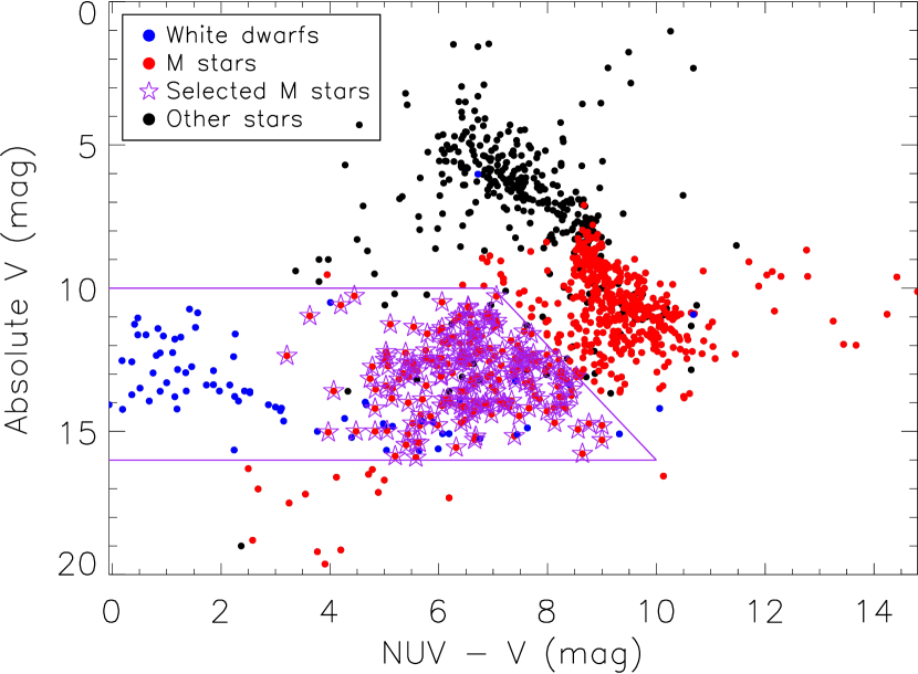
Figure 1.— $V$ / $NUV-V$ magnitude - color diagram of the stars in the Gliese catalog within 20 pc of the sun. M stars are shown in red, single WDs (including additions from the Holberg et al. 2008 catalog) are shown in blue and other stars are shown in black. The purple line illustrates our color cut and purple stars are the 138 M stars out of which our targets were selected.

II.2. Observations and Data Reduction

The observations were performed with the X-Shooter spectrograph mounted at the Kueyen unit of the Very Large Telescope (UT2), operated by the European Southern Observatory (ESO) on Cerro Paranal in Chile (Program IDs 095_D-0949(A) and 096_D-0963(A), PI: Paul Vreeswijk). X-Shooter records spectra with three separate arms simultaneously - UVB, VIS and NIR. This allows a wide wavelength range (3000-25000 Å) while maintaining good sensitivity throughout this range (Vernet et al., 2011). In particular, the instrument is very blue-sensitive down to the atmospheric cutoff around 3000 Å. Thus, we benefit from the ability to characterize the dM spectrum in the red part while allowing possible detection of WD contribution in the blue part. Since out targets are very bright, our observation plan was submitted to ESO as a ”filler” program, to be executed during poor seeing conditions (>1.5″). We obtained service-mode observations with VLT/X-Shooter for 60 (41) targets during ESO Period 95 (96), securing spectra of a total of 101 dMs. Corrected locations of all targets were calculated using proper motions from the Stauffer et al. (2010) 2MASS-Gliese cross-correlation catalog. Exposure times were typically 120 s for UVB, 90 s for VIS and four separate exposures of 30 s each for NIR. In some cases, exposure times were increased for faint targets or decreased to prevent saturation of the detector. Moreover, saturation was avoided for bright targets ($M_{V}\sim 10$) by using a 1x1 binning read-out mode instead of 1x2. All of the observations were made in Stare mode using the widest 5.0″ slit, to increase the chances of including a WD companion in the spectrum (up to separation of 40 AU for a 16 pc target, the distance at half the 20 pc volume). The resolving power of X-Shooter for the 5.0″ slit was measured to be about 5000, 9000 and 5000 for the UVB, VIS and NIR arms, respectively. This was done by examining several unresolved lines in the spectra and dividing their wavelengths by their full width at half maximum (FWHM).

Spectra were reduced using ESO’s Reflex pipeline version 2.8 (Freudling et al., 2013). A built-in ”optimal extraction” algorithm (Horne, 1986) was used to increase Signal-to-noise ratio (SNR). For the UVB and VIS arms, optimal extraction yielded a mean improvement of 5 and 4 percent in SNR, respectively, compared to standard extraction. On the other hand, for the NIR arm a mean 4 percent decrease in SNR was noted, with artifacts introduced to some of the spectra. Thus, we have decided to use optimal extraction for the UVB and VIS arms only, and standard extraction for the NIR arm.

We removed very noisy parts in the UVB and VIS arms below 3200 and 5500 Å, respectively. The three spectral pieces were then stitched together using overlap regions as reference. Both the UVB and the VIS spectra include a feature at $\sim$5500-5800 Å due to the dichroic splitter of X-Shooter (Chen et al., 2014). Thus, we excluded this feature from the overlap regions.

The pipeline produces a flux-calibrated spectrum for each target using a spectroscopic standard star that was observed on the same night. This procedure assumes photometric nights. Therefore, we performed absolute calibration for each object using JHK band photometry from the 2MASS catalog (Skrutskie et al., 2006), since these are the only bands that are reported for all of our targets in the SIMBAD database (Wenger et al., 2000). We calculated JHK synthetic photometry for each spectrum and rescaled the flux to match the photometric data.

The log of spectroscopic observations is presented in Table 2 in the appendix, along with plots of the reduced spectra. These are also available on the WISeREP repository (Yaron & Gal-Yam, 2012) and are searchable via object name or by type ”M dwarf”.

III. Results and Analysis

III.1. Activity and Multiplicity

Out of the 101 observed targets, 65 show strong emission lines that are indicative of magnetic activity: the hydrogen Balmer series and the Ca II H and K lines (see Reid & Hawley, 2005). An example of these lines for target GJ2069 is shown in Fig. 2. The remainder of the targets show little or no emission lines. Five spectra are showing double emission lines (also shown in Fig. 2), which suggests that these are in fact binary stars which are not listed in the Gliese catalog. A search of binary star catalogs (Mason et al. 2001 and Shkolnik et al. 2010) shows that indeed these are known binary or higher multiplicity systems, and revealed 21 additional multiples in our sample with separations smaller than half of our slit width (targets were positioned in the center of the slit) that were not filtered out initially. The separations of these systems are listed in Table 1 and we give special care to these in our analysis later on.

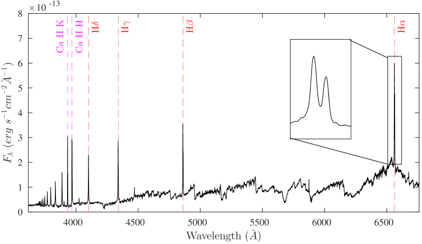
Figure 2.— Example emission lines for GJ2069. In red - the first four Balmer series lines. In pink - Ca II H/K lines. The double H $\alpha$ line is shown in the inset.

III.2. White Dwarf Spectral Features

According to the Kleinman et al. (2013) SDSS survey, over 90% of WDs are classified as having either hydrogen or helium atmospheres, indicating a spectral type of DA or DB, respectively. Thus, we first visually examine the spectrum of each target in search of distinct broad absorption features typical of these spectroscopic classes. For type DA these would be the hydrogen Balmer lines at 6563 Å, 4861 Å, 4341 Å and 3970 Å. For type DB the dominant lines are from neutral helium at 4026 Å, 4471 Å and 5875 Å (Bergeron et al., 2011). Some WDs show only a continuum spectrum - type DC. According to Giammichele et al. (2012), those can be hydrogen atmosphere WDs of $T_{\textrm{eff}}\leq 5000\,K$ or helium atmosphere WDs of $T_{\textrm{eff}}\leq 12000\,K$. The search for this type and other more exotic types was done by looking for a clear rise in the blue part of each target. No evidence for DA or DB features, nor of a clear UV rise, was found in any of the spectra.

III.3. Limits on the Temperature of Unseen WDs

Next, we place upper limits on the effective temperature of WDs that may still be hiding below our detection threshold. We do so by modeling spectra of WDs with a mass of $0.6\,\mbox{M${}_{\odot}$}$ as black-bodies of varying effective temperatures. We use this mass value as it is the peak of the narrow observed WD mass distribution (see Bergeron et al. 2001, Kepler et al. 2007). Using these models and spectral templates for each dM, we determine at which temperature the WD models can be rejected.

As spectral dM templates, we tried to use the Pickles (1998) spectral library, which did not provide good enough fits to our data due to the low resolution ($\sim$500 Å) and to a limited number of spectral subtypes. We have also tried using the PHOENIX synthetic spectral models (Husser et al., 2013), which did not describe our data well in the UVB and NIR parts. Eventually, we have decided to use our own data as templates, under the assumption that most of our targets do not hide WD companions. Indeed, the self-template method yields better fits for the vast majority of our targets (see electronic Figs. 5 to 79), compared with the alternative methods.

The best fitting template for each target was determined as the one with the lowest Residual Sum of Squares (RSS) score:

$$\textrm{RSS}=\sum_{i}(f_{S,i}-f_{T,i})^{2}$$ (1)

where $f_{S,i},f_{T,i}$ are the flux values of the current target and of each template, respectively. Before calculating the RSS score, the spectra were rescaled to each other such that the flux integral is equal to one. We excluded from the fit the blue part below 6300 Å to minimize possible WD contamination, while keeping the prominent dM features that extend to redder wavelengths. We also excluded wavelength ranges of known telluric features at: 6340-6420 Å, 6840-6960 Å, 7147-7323 Å, 7575-7705 Å, 8130-8365 Å, 8939-9240 Å, 9280-9830 Å, 10810-11710 Å, 12670-12710 Å, 13000-15030 Å, 17350-19810 Å, 19950-20350 Å and 20480-20820 Å (Moehler et al., 2014). As we only have 101 spectra to work with, dividing them into magnetically active and non-active would limit our ability to find good templates. Thus, we included both active and non-active stars in the template bank for all targets while excluding the Balmer H $\alpha$ line from the fit range. As shown, for example, in Fig. 13, nice fits are produced also when using active templates for non-active targets and vice versa.

As white dwarf synthetic spectra were not available to us, we chose to model WDs as black-bodies of varying effective temperatures and with radii that fit a typical mass of $0.6\,\mbox{M${}_{\odot}$}$. The radius for each $T_{\textrm{eff}}$ value was calculated using $R^{2}=GM/g$ and the surface gravity ($\log g$) values from the publicly available WD color model grids of Holberg & Bergeron (2006), Kowalski & Saumon (2006), Tremblay et al. (2011) and Bergeron et al. (2011). Absolute flux values of the models were calculated using these radii and the distances to each target, obtained from the Gliese catalog.

Next, we determine the hottest WD that may be hiding in the data for each target. The dM fits are not perfect and exhibit correlated residuals (i.e. spectral regions which are systematically lower or higher between each target and its template). Such correlated noise make it very difficult to make quantitative statements. We attempt to explain the observed spectrum using a combination of the template spectrum and an approximate WD model, and to ask when the temperature of the WD produces a ”noticeable” effect on the composed spectrum. In each such fit, the WD flux is completely determined by its radius (assuming a $0.6\,\mbox{M${}_{\odot}$}$ WD), its distance, and assuming a black-body emitter. Therefore, we use several methods to put limits on the WD temperature that can be hidden in each system. We note that since the WD luminosity is very sensitive to its effective temperature (i.e. $\propto T_{\textrm{eff}}^{4}$), any reasonable estimator will yield similar results regardless of the details of the test.

In the first method, we reject WD models which yield an RSS score double than that of the template alone. We add the flux of the best fit template to the black-body models for a grid of effective temperatures between 1500 K and 20000 K, and calculate the RSS score for each temperature. We then compare these scores with the RSS of the fit with no WD. The lowest temperature for which the RSS score is more than double the score without the model is set as our upper limit. This test is arbitrary, but due to the extreme sensitivity of the luminosity on $T_{\textrm{eff}}$, the obtained limits are similar for different criteria. For example, changing the threshold to 3 times the RSS yields an average increase in limit temperature of only 400 K. Our temperature grid follows that of the color models - from 1500 to 5500 K in steps of 250 K and then to 15000 K in steps of 500 K. As opposed to the template fitting, we now calculate the RSS score for wavelengths 3200-10000 Å, where WD contribution would be dominant. In addition to the H $\alpha$ line and tellurics, we also remove from the fit range the rest of the Balmer emission lines, the Ca II lines and the X-Shooter dichroic feature.

In the second method, we reject WD models which exceed the fit residuals envelope. The envelope is defined as the 99th percentile of the flux for the absolute value of the fit residuals. In this case, the limit is set as the lowest temperature for which the black-body model flux exceeds the envelope. In other words, the rejected WD model is the coldest one which is not consistent with the residuals of the fit.

The third method is robust and template-independent. Here, we compare the integrated flux of the very blue part of the dM spectra to that of our black-body models. The limit is set as the temperature of the coldest model for which the total UV flux is greater than that of the dM. This was done for wavelengths of 3200-3700 Å, as this range features only a weak continuum from the dMs. In addition, this range is bluer than the Balmer series, thus avoiding the typical absorption features of WDs and ensuring that black-body is a good approximation for WD spectra. An example of the three methods is given in Fig. 3.

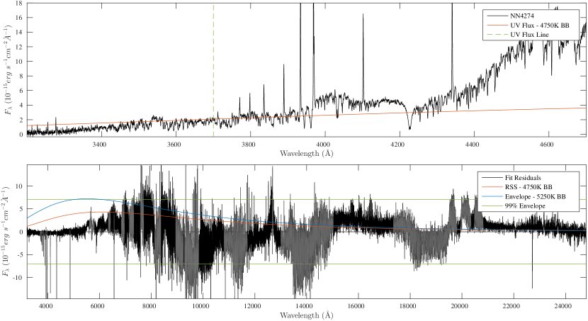
Figure 3.— Example of limit calculations for NN4274. Top panel: The UV part of the spectrum is shown in black. In orange - the rejected black-body model from the UV flux method. In green - The 3700 Å line defining the UV flux region. Bottom panel: The fit residuals from the best fit template GJ1154 are shown in black. In orange and blue are the rejected black-body models from the RSS and envelope methods, respectively. In green - the 99% flux envelope.

To verify that the black-body model describes WDs well enough for our purposes, we repeat the analysis using spectra derived from photometry of the color models. For each effective temperature, we calculate flux values from the UBVRI band photometry using:

$$F_{\lambda}=F_{\lambda,0}\cdot 10^{(-0.4M_{\lambda})}\cdot(10/D)^{2}$$ (2)

Where $M_{\lambda}$ are the UBVRI magnitudes, $F_{0}$ are vega zero point fluxes calculated in Holberg & Bergeron (2006) and D is the distance to each target, which is used to normalize the flux as the magnitudes were calculated for 10 pc, i.e. absolute magnitudes. The wavelength of each flux value is taken as the effective wavelength of each band, also reported in Holberg & Bergeron (2006). We then interpolate between these points to obtain a model spectrum. We do this for the hydrogen-atmosphere and the helium-atmosphere color models. Both hydrogen and helium models yield the same limits as the black-body model up to 500 K differences in effective temperature, showing that indeed using the black-body approximation is good enough for our analysis.

As noted before, 26 of our targets are listed in binary catalogs as binaries or higher multiplicity systems with separations of less than 2.5″ (close binaries, hereafter), which is within half the X-Shooter slit width that we have used. Five of those display double emission lines in their spectra. The spectra of the rest of these close binaries may or may not contain more than one star. Thus, they are problematic for our limit analysis and must be analyzed with care. As a first precaution, we have taken these targets out of the template bank. Second, for these cases we only report the limits obtained using the UV flux method, which is independent of template.

The limits obtained and best fit templates for each target are listed in Table 1. Electronic Figs. 5 to 79 display, for each target:

1. The spectrum.

2. The best fit template, rescaled to the flux of the target.

3. The residuals of the fit and the rejected black-body models used to derive the limits.

Figures 80 and following display the spectra of the close-binary targets, for which no template analysis was performed.

Table 1Obtained results of spectral analysis

Name	Template	RSS	Env.	UV Flux	Act.	Sep.
		[K]	[K]	[K]		[″]
NN3010				5250	V	0.1
NN3017	GJ2021	5250	6500	5250	V
NN3027	NN3682	5250	6500	5500	V
NN3033	NN3518	5000	6500	4750	V
NN3034	GJ1204	5000	6500	5000
NN3039				6000	V	0.7
GJ1019	NN3227	6000	6000	5000
NN3056	NN3142	4500	6000	5250
GJ1024	GJ1031	6000	7000	5500
GJ1029	NN3937	4750	6000	3750
GJ1031	NN3225	5000	5500	5250	V
GJ2021	GJ1031	4500	5500	4750
NN3076				4250	V	0.3
NN3119	NN4292	4000	5000	4250	V
Gl83.1	NN3225	4000	5000	4750	V
NN3129				5500	D
NN3142	NN3149	5250	7000	5500	V
NN3143	Gl828	6000	6500	5500	V
NN3149	GJ1031	6000	7000	6500	V
NN3148	GJ1284	6500	8000	6500	V
Gl102	GJ1031	5250	6500	5250
GJ1055	NN3253	3750	5000	4250
NN3224				4500	D	0.3+2
NN3225	Gl83.1	4500	5250	4000	V
NN3227	Gl729	7500	7000	6000	V
NN3237	NN3253	6500	6500	5500	V
NN3253	NN3237	4500	5500	4500
NN3261				6500	V	0.8
NN3296	NN3225	5500	6000	5000	V
NN3304				5500	V	1.1
NN3322				6500	V	1.4
NN3326	NN3967	6000	6500	5250	V
NN3332				8000	V	0.8
NN3344	Gl207.1	10000	9500	8500
Gl207.1	GJ1284	10500	9500	8000	V
GJ1083				4000	V	0.5
NN3405	Gl828	6500	7500	6000
GJ1093	GJ1286	4000	5250	3750
NN3423	Gl729	5500	6500	5500	V
GJ1096	NN3225	5000	6000	4500	V
Gl268.3				6500		0.1
NN3454				4750	V	0.3
NN3463	GJ1103	4250	5250	4750
GJ1103	NN3463	5500	5500	5000
NN3466				5500		1
GJ1108				7500	D	0.3+14
Gl300				5250		2
NN3503	NN3518	4500	5500	4250
GJ2069				7000	D	1+10+22
Gl324	NN3967	6500	7000	5500
NN3518	NN3033	5000	6000	5000	V
GJ1116				3750	V	1.8
NN3543	NN3344	8500	8000	6500	Ca
NN3549	NN3937	4000	5250	4250	V
Gl347	GJ1031	5250	6000	4500
Gl359	Gl347	4500	6000	4500
NN3571	Gl347	4750	6000	4750	V
NN3572	GJ1186	8500	8000	6500
NN3573	NN3571	7000	7500	5000
NN3590	GJ1186	6000	7500	5000
NN3647	GJ1031	6000	8000	6500
NN3654	Gl781.1	7000	7500	5500
NN3657	GJ1031	4250	6000	4250
NN3668	NN3463	4500	6000	4750
NN3682	NN3780	6000	6500	6000	V
NN3685	NN3149	6500	7000	6000	V
GJ1154	NN3149	4250	5500	4750	V
NN3780	NN3682	6000	6500	6000	V
GJ1179	NN3682	4750	5250	3750	V
NN3808	GJ2021	6000	6500	5000	V
Gl540.2	NN4292	5500	6500	5250	V
NN3856	NN3780	5250	6500	5500	V
GJ1186	NN4292	5250	5500	4500
NN3900	Gl828	5500	7000	6000
NN3937	GJ1029	4750	5500	4250
GJ1204	GJ1284	6000	6500	5250	V
NN3967	NN3326	4500	6000	5000	V
NN3981				5500	V	0.6
GJ1210				4750	V	0.4
NN4032	NN3227	8500	8000	6500
NN4071	NN3423	6000	7000	5500	V
Gl729	NN3227	4750	6000	5250	V
Gl781.1	NN4279	7500	8000	7000	V
Gl791.2				5000	V	0+0.2
Gl828	NN3143	4750	6500	5500
NN4201				5500	V	0.8
Gl836	NN4071	6000	6500	6000
NN4215	NN4292	4500	5500	4500
NN4231				7500	V	0.2+0.7
NN4239	NN3657	5250	6000	4500
NN4274	GJ1154	4750	5250	4750	V
NN4279	Gl781.1	5000	6000	5500	V
NN4282				7500	V	1.5
NN4292	NN3119	5500	5500	4500	V
NN4302	Gl781.1	6000	6500	5500
NN4326				6500	V	0.1
GJ1284	Gl83.1	9500	9000	7500	V
GJ1286	Gl207.1	5000	5250	4000
NN4360				4500	V	0.6
NN4362	GJ1284	7500	8000	7000	V
NN4378				7000	D	0.6+20

Note. — RSS, Env. and UV Flux are the limits obtained using the three methods. Targets without reported templates and RSS/Envelope limits are those defined as close binaries.

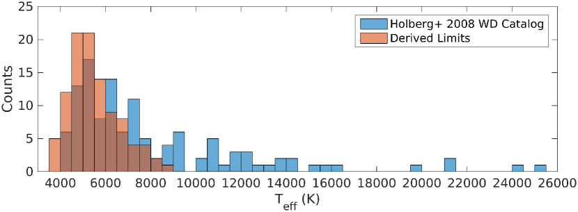
Figure 4.— The effective temperature distributions of the limits derived in this study and of the WDs in the Holberg et al. (2008) catalog.

IV. DISCUSSION

Motivated by the evidence for missing WDs in multiple systems, we have used X-Shooter to record spectra of 101 dMs which show NUV excess. We have examined these spectra for evidence of WD spectral features. When those were not found, we have used the spectra themselves as templates, modeled WDs as black-bodies and obtained upper limits for the effective temperatures of WDs that may still be hidden, using three different methods. It is important to note that the limits obtained are only within our slit width of 5″. Since our targets are positioned roughly at the center of the slit, this corresponds to a companion at 40 AU for a target at 16 pc (the distance at half the 20 pc volume). Though our slit is only 5″ wide, it is 11″ long, which could allow a companion at larger separations. Thus, we take order $\sim$50 AU as our typical separation limit.

Figure 4 shows the effective temperature distribution of our derived limits, selected as the tightest limit for each target among the three methods. Also shown is the effective temperature distribution of WDs in the Holberg et al. (2008) catalog. According to these, our limit analysis is sensitive to $\sim$75% of WDs in the local volume. The average obtained limit for our 101 dM sample is 5300 K. Thus, the frequency of dM-WD binaries with WD hotter than that is smaller than 3% at the 95% confidence level.

The Gliese catalog lists $\sim$1900 non-WD stars with distances below 20 pc. Assuming that 100 WD companions are missing from that volume (Katz et al., 2014) and that WDs do not prefer specific class of companions, then 5% of the stars should have WD companions. As we have detected no WDs in our 101 dM sample, this hypothesis can be rejected at the 99.3% confidence level. However, our survey is sensitive to WDs hotter than $\sim$5300 K, corresponding to $\sim$75% of the known local population. In addition, our slit width limits our survey to separations of order $\lesssim 50$ AU, which corresponds to 55% of dM-WD pairs (Farihi et al., 2010). Taking both into account, the expectancy is to detect only two WDs in our sample, and this hypothesis can be rejected at the 86% confidence level. The missing WDs may be colder than our detection limit or outside our slit, thus undetected. Another possibility is that the missing WDs are not hidden in the shadow of dMs, but rather are companions to stars of earlier types, as proposed in Ferrario (2012). Or else, perhaps not as many WDs are missing from the local volume as claimed.

It is interesting to note that selecting targets according to NUV excess produced a strong bias towards active dMs. For example, for spectral types M4 and M5, which make up the majority of our sample, we noted a 62% activity fraction, as opposed to $\sim$35% for the SDSS survey of West et al. (2004). Studies of magnetic activity of dMs can thus benefit from our data set.

As mentioned before, our spectra are available online for public use. In our observations, we covered the entire wavelength range of active and non-active dMs at medium resolution, including several binaries with resolved double emission lines. We hope that this data will be useful for future research.

The appendix contains Table 2 of the observation log, Figs. 5 to 79 which contain the spectra, the best fit templates, the fit residuals and black-body models of the derived limits. Excluded fit ranges of tellurics, emission lines and dichroic feature are colored in gray. Also included are Figs. 80 and following, which display the spectra of the close binary targets.

Table 2Observed M dwarfs

Name	RA	DEC	Spectral	$M_{V}$	Distance	Observation	Observation	Airmass	Seeing	UVB Exposure	VIS Exposure	NIR Exposure
			Type		[pc]	Date	UT Time	[″]	[″]	[s]	[s]	[s]
NN3010	00:08:53.95	+20:50:22.4	M5	13.54	10.64	2015-07-16	09:54:56	1.452	0.9	120	90	4x30
NN3017	00:15:36.88	-29:46:02.7	M4	14.31	17.86	2015-08-13	05:25:54	1.138	1.5	120	90	4x30
NN3027	00:18:54.11	+27:48:47.4	M4	13.86	19.23	2015-10-30	00:41:26	1.914	1.2	120	90	4x30
NN3033	00:24:35.78	+30:02:30.2	M5	14.54	18.87	2015-10-30	01:03:07	1.937	1.1	120	90	4x30
NN3034	00:25:20.42	+22:53:04.0	M4	14.30	18.87	2015-06-20	10:06:16	1.566	1.1	120	90	4x30
NN3039	00:32:34.97	+07:29:25.3	M4	12.70	11.63	2015-07-25	08:58:25	1.182	1.1	120	90	4x30
GJ1019	00:43:35.52	+26:28:25.1	M4	14.52	19.27	2015-10-14	05:33:38	1.886	1.1	120	90	4x30
NN3056	00:47:08.22	-23:30:31.1	M3	14.40	18.52	2015-08-13	05:47:17	1.169	1.6	120	90	4x30
GJ1024	00:56:39.19	+17:27:30.3	M4	13.71	17.42	2015-07-25	08:49:12	1.371	1.1	120	90	4x30
GJ1029	01:05:39.95	+28:29:31.3	M5	14.80	12.56	2015-10-14	06:01:32	1.919	1.2	120	90	4x30
GJ1031	01:08:19.12	-28:48:23.6	M3	13.42	13.16	2015-08-13	05:33:08	1.277	1.2	120	90	4x30
GJ2021	01:09:19.02	-24:4x30:28.3	M4	14.52	15.38	2015-08-13	05:40:14	1.262	1.3	120	90	4x30
NN3076	01:11:25.65	+15:26:18.5	M5	14.36	8.47	2015-07-25	07:50:46	1.510	1.2	120	90	4x30
NN3119	01:51:04.76	-06:07:10.0	M4.5	14.60	10.00	2015-07-25	09:23:14	1.089	1.0	120	90	4x30
Gl83.1	02:00:14.15	+13:02:38.3	M4	12.28	4.47	2015-07-25	08:03:38	1.631	1.2	120	90	4x30
NN3129	02:02:44.89	+13:34:4x30.9	M4.5	14.27	17.24	2015-07-25	08:19:09	1.570	1.2	120	90	4x30
NN3142	02:12:55.31	+00:00:17.3	M4	13.50	16.67	2015-07-25	09:33:35	1.155	0.9	120	90	4x30
NN3143	02:15:34.75	+33:57:34.9	M3.5	13.58	17.24	2015-10-13	05:53:42	1.929	1.0	120	90	4x30
NN3149	02:16:35.90	-30:58:05.4	M4	13.00	11.36	2015-08-13	06:10:58	1.409	1.0	120	90	4x30
NN3148	02:16:41.99	-4x30:59:15.8	M3	12.00	11.36	2015-08-13	06:03:07	1.453	1.0	120	90	4x30
Gl102	02:33:37.24	+24:55:27.3	M3.5	12.96	9.77	2015-07-25	09:50:28	1.651	0.8	120	90	4x30
GJ1055	03:09:00.59	+10:01:16.4	M5	14.85	11.88	2015-12-15	04:41:59	1.536	0.8	120	90	4x30
NN3224	03:25:42.18	+05:51:50.4	M4.5	14.70	12.99	2015-12-15	04:50:56	1.417	0.8	120	90	4x30
NN3225	03:26:45.08	+19:14:39.3	M4.5	14.96	16.67	2015-10-11	09:23:10	1.855	1.0	120	90	4x30
NN3227	03:28:49.89	+26:29:10.3	M4	13.40	18.18	2015-10-11	08:01:56	1.689	0.4	120	90	4x30
NN3237	03:36:41.04	+03:29:17.5	M5	13.86	14.29	2015-12-15	04:59:38	1.369	0.8	120	90	4x30
NN3253	03:52:42.29	+17:00:55.0	M5	13.70	9.62	2015-10-14	06:27:09	1.360	0.8	120	90	4x30
NN3261	04:05:38.91	+05:44:40.3	M3.5	12.89	15.87	2015-12-15	05:07:15	1.325	0.8	120	90	4x30
NN3296	04:33:34.62	+20:44:41.7	M5	14.60	15.63	2015-10-14	07:22:20	1.432	1.2	120	90	4x30
NN3304	04:38:13.13	+28:12:58.7	M4.5	12.53	10.00	2015-10-13	07:31:23	1.665	1.0	120	90	4x30
NN3322	05:01:58.86	+09:58:57.7	M3.5	11.47	7.04	2015-12-17	05:47:09	1.367	0.7	120	90	4x30
NN3326	05:04:14.67	+11:03:27.3	M5	13.75	13.70	2015-12-17	05:58:45	1.419	0.6	120	90	4x30
NN3332	05:06:49.54	-21:35:04.8	M3	11.66	12.05	2015-10-21	06:26:10	1.063	1.1	60	45	4x15
NN3344	05:16:00.36	-72:13:59.7	M2	11.70	19.23	2015-10-21	06:35:03	1.523	0.8	120	90	4x30
Gl207.1	05:33:44.55	+01:56:39.5	M3	11.53	15.08	2015-12-17	05:37:45	1.163	0.6	60	45	4x10
GJ1083	05:40:25.91	+24:48:02.3	M7	14.85	10.34	2015-10-11	08:28:00	1.560	1.3	120	90	4x30
NN3405	06:42:13.46	+03:35:26.5	M4	13.33	15.63	2015-12-17	06:29:22	1.159	0.7	120	90	4x30
GJ1093	06:59:29.95	+19:20:41.0	M5	14.83	7.76	2015-10-11	08:48:44	1.542	1.0	120	90	4x30
NN3423	07:03:23.25	+34:41:54.9	M4	13.17	13.33	2015-11-06	08:31:36	1.957	1.1	120	90	4x30
GJ1096	07:16:18.07	+33:09:03.8	M5	14.48	14.90	2015-11-07	08:40:59	1.873	1.1	120	90	4x30
Gl268.3	07:16:19.93	+27:08:29.8	M3	10.85	7.94	2015-10-11	08:59:03	1.842	0.8	120	90	4x10
NN3454	07:36:25.38	+07:04:38.6	M4.5	13.22	6.17	2015-12-17	06:37:36	1.174	0.6	120	90	4x30
NN3463	07:51:51.87	+05:32:51.1	M4.5	14.75	15.92	2015-12-07	07:59:18	1.165	0.7	120	90	4x30
GJ1103	07:51:54.99	-00:00:23.2	M4.5	13.50	8.79	2015-12-07	08:26:09	1.132	0.8	120	90	4x30
NN3466	07:54:55.22	-29:21:04.4	M4	13.38	12.50	2015-10-21	07:08:15	1.462	0.8	120	90	4x30
GJ1108	08:08:55.43	+32:49:02.6	M2.8+M3.3	12.12	17.24	2015-12-06	08:05:23	1.855	0.9	120	90	4x20
Gl300	08:12:40.98	-21:33:18.1	M3.5	12.10	5.88	2015-10-21	06:57:12	1.734	0.7	120	90	4x30
NN3503	08:31:22.82	-10:29:59.9	M4	15.00	15.38	2015-10-21	07:25:13	1.802	1.1	120	90	4x30
GJ2069	08:31:37.48	+19:23:37.5	M5	11.89	8.77	2015-11-19	07:33:41	1.596	1.0	120	90	4x30
Gl324	08:52:40.41	+28:18:55.5	M4	13.14	13.09	2015-12-09	07:47:06	1.683	0.8	120	90	4x30
NN3518	08:55:19.62	-23:52:14.1	M4	14.00	12.20	2015-10-21	07:32:49	1.776	0.9	120	90	4x30
GJ1116	08:58:14.39	+19:45:46.1	M5.5	14.06	5.23	2015-11-19	07:14:53	1.883	1.0	120	90	4x30
NN3543	09:16:20.35	-18:37:31.3	M2	10.75	12.50	2015-04-15	00:09:21	1.008	0.5	120	70	4x10
NN3549	09:18:41.36	+26:45:46.4	M5	16.00	20.00	2015-12-09	08:12:52	1.625	1.0	120	90	4x30
Gl347	09:28:55.54	-07:22:22.0	M4.5	15.00	16.72	2015-05-19	01:03:31	1.332	1.2	120	90	4x30
Gl359	09:41:02.70	+22:01:21.0	M4.5	14.23	12.17	2015-04-09	23:55:43	1.557	0.8	120	90	4x30
NN3571	09:53:54.82	+20:56:52.2	M4	14.05	10.20	2015-04-14	23:41:40	1.548	0.4	120	90	4x30
NN3572	09:55:43.61	+35:21:41.7	M3.5	12.73	17.54	2016-02-04	07:13:20	2.241	0.8	120	90	4x30
NN3573	09:56:26.53	+22:38:57.9	M4	14.20	16.13	2015-04-12	01:24:52	1.470	0.7	120	90	4x30
NN3590	10:15:06.93	+31:25:08.7	M4	13.60	18.18	2015-12-14	08:15:25	1.909	0.7	120	90	4x30
NN3647	11:11:51.74	+32:33:11.4	M3.5	12.38	12.20	2016-02-03	08:53:00	2.250	0.8	120	90	4x30
NN3654	11:16:37.08	-27:57:30.5	M3.5	13.70	15.63	2015-05-17	02:22:37	1.126	0.9	120	90	4x30
NN3657	11:23:07.96	+25:53:36.8	M5	15.14	17.33	2016-02-05	05:55:29	1.668	0.8	120	90	4x30
NN3668	11:31:08.78	-14:57:41.2	M5	14.29	12.82	2015-07-15	23:42:57	1.388	0.7	120	90	4x30
NN3682	11:43:23.43	+25:18:13.5	M4	13.83	18.87	2015-05-19	00:52:43	1.551	1.1	120	90	4x30
NN3685	11:47:40.46	+00:15:19.7	M4	13.25	15.63	2015-07-15	23:50:34	1.520	0.9	120	90	4x30
GJ1154	12:14:15.60	+00:37:22.9	M4.5	13.73	8.46	2015-07-16	00:00:32	1.431	1.0	120	90	4x30
NN3780	13:23:37.34	-25:54:47.8	M3.5	12.90	12.66	2015-08-10	23:35:04	1.256	1.2	120	90	4x30
GJ1179	13:48:11.82	+23:36:50.9	M5	15.32	11.99	2015-07-16	00:08:44	1.595	0.9	120	90	4x30
NN3808	13:48:48.66	+04:06:00.9	M4	14.34	16.39	2015-08-13	23:26:41	1.417	1.3	120	90	4x30
Gl540.2	14:13:04.24	-12:01:31.5	M5	13.86	11.63	2015-08-13	23:36:29	1.192	0.9	120	90	4x30
NN3856	14:32:11.01	+16:00:49.1	M5	13.61	14.93	2015-04-21	06:55:55	1.465	0.8	120	90	4x30
GJ1186	14:53:37.31	+11:34:02.2	M4.5	15.29	18.55	2015-04-21	07:42:35	1.463	0.9	120	90	4x30
NN3900	15:19:11.00	-12:45:08.2	M4	12.58	13.33	2015-06-12	03:50:18	1.065	0.9	120	90	4x30
NN3937	16:04:20.00	-06:16:57.8	M4.5	15.51	16.56	2015-04-21	08:12:07	1.120	0.7	120	90	4x30
GJ1204	16:36:05.18	+08:48:47.7	M4	13.80	15.34	2015-06-12	04:52:04	1.234	0.8	120	90	4x30
NN3967	16:40:06.23	+00:42:16.9	M5	13.69	11.20	2015-06-12	04:09:01	1.106	0.8	120	90	4x30
NN3981	16:58:24.94	+13:58:11.5	M4	13.13	12.99	2015-04-02	09:25:52	1.288	0.8	120	90	4x30
GJ1210	17:07:40.42	+07:22:01.7	M5	14.01	12.82	2015-06-12	05:02:54	1.192	0.7	120	90	4x30
NN4032	17:53:00.42	+16:54:59.3	M3.5	12.69	17.54	2015-04-21	07:20:12	1.432	0.9	120	90	4x30
NN4071	18:42:45.07	+13:54:22.0	M5	12.81	10.42	2015-04-21	07:32:02	1.491	0.8	120	90	4x30
Gl729	18:49:50.13	-23:50:14.4	M3.5	10.46	2.93	2015-06-12	04:42:07	1.067	0.8	120	30	4x10
Gl781.1	20:07:45.27	-31:45:24.9	M4	12.50	19.72	2015-06-17	10:09:34	1.307	0.8	120	90	4x30
Gl791.2	20:29:49.07	+09:41:23.1	M4.5	13.05	8.76	2015-06-17	09:44:17	1.473	0.6	120	90	4x30
Gl828	21:26:53.22	-44:48:44.6	M3.5	14.10	14.93	2015-07-13	04:56:12	1.155	1.1	360	300	4x100
NN4201	21:32:22.36	+24:33:42.0	M4	12.66	12.35	2015-05-28	09:50:41	1.530	0.3	120	90	4x30
Gl836	21:39:02.08	-24:09:40.8	M4	13.43	13.95	2015-07-13	05:11:28	1.097	0.8	360	300	4x60
NN4215	21:44:08.31	+17:04:38.2	M4.5	14.81	17.54	2015-06-15	09:49:04	1.387	0.9	120	90	4x30
NN4231	21:52:10.59	+05:37:33.7	M2.4	12.11	15.63	2015-05-22	09:38:37	1.197	0.8	120	90	4x30
NN4239	21:56:56.63	-01:54:00.5	M5	14.64	13.33	2015-07-13	04:38:48	1.397	1.1	360	300	4x100
NN4274	22:23:07.34	-17:36:36.2	M4.5	13.25	7.46	2015-09-09	04:51:51	1.036	0.9	120	90	4x30
NN4279	22:27:03.07	+06:49:33.4	M3.5	13.22	13.89	2015-09-09	05:01:00	1.222	1.0	120	90	4x30
NN4282	22:33:22.92	-09:36:53.0	M3	12.41	16.95	2015-09-09	05:09:45	1.076	0.8	120	90	4x30
NN4292	22:43:23.71	+22:08:17.8	M5	15.00	15.87	2015-07-25	07:26:48	1.463	1.3	120	90	4x30
NN4302	22:54:47.15	-05:28:19.8	M4	13.90	20.00	2015-08-21	08:55:18	1.574	0.8	120	90	4x30
NN4326	23:17:28.57	+19:36:46.2	M2	12.10	12.82	2015-07-25	08:39:29	1.438	1.1	120	90	4x30
GJ1284	23:30:13.82	-20:23:29.3	M2	11.16	10.87	2015-09-09	05:36:07	1.013	0.8	100	75	4x15
GJ1286	23:35:11.31	-02:23:33.4	M5	14.69	7.22	2015-09-09	05:47:55	1.099	0.7	120	90	4x30
NN4360	23:45:30.87	-16:10:27.5	M5	14.50	9.01	2015-09-09	05:56:39	1.025	0.6	120	90	4x30
NN4362	23:48:35.42	-27:39:44.4	M2.5	12.40	18.87	2015-08-13	05:54:23	1.042	1.3	120	90	4x30
NN4378	23:57:20.84	-12:58:47.4	M4	12.93	17.86	2015-09-09	06:07:33	1.035	0.6	120	90	4x30

Note. — Observed M dwarfs, ordered by RA. Spectral types are from SIMBAD (Wenger et al., 2000), distances are from the Gliese catalog

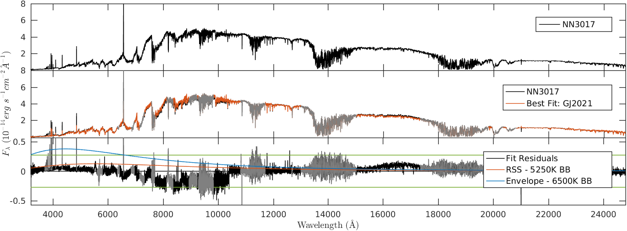
Figure 5.— NN3017

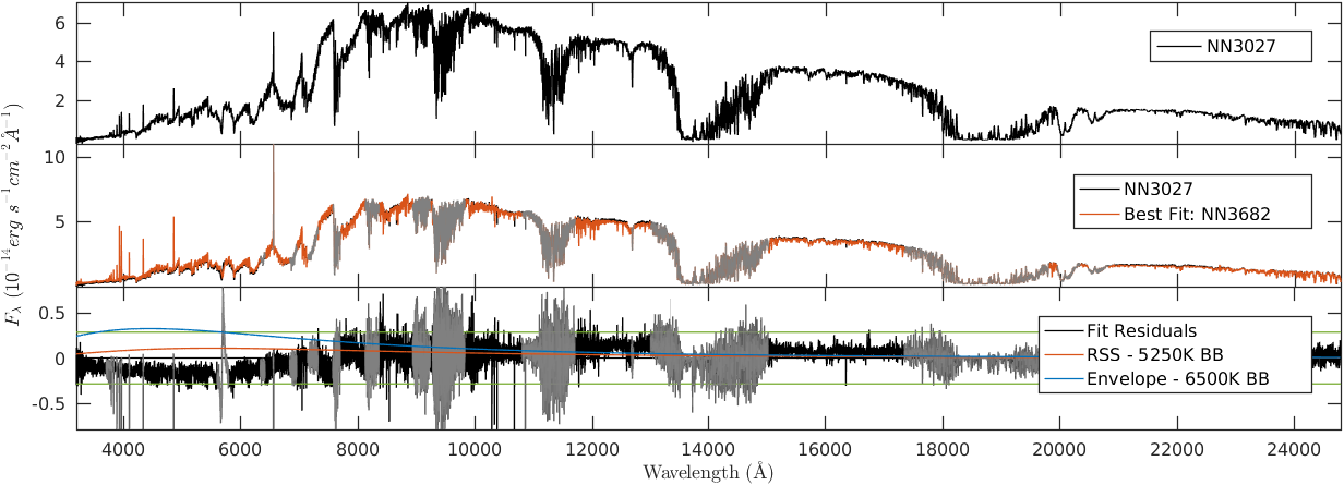
Figure 6.— NN3027

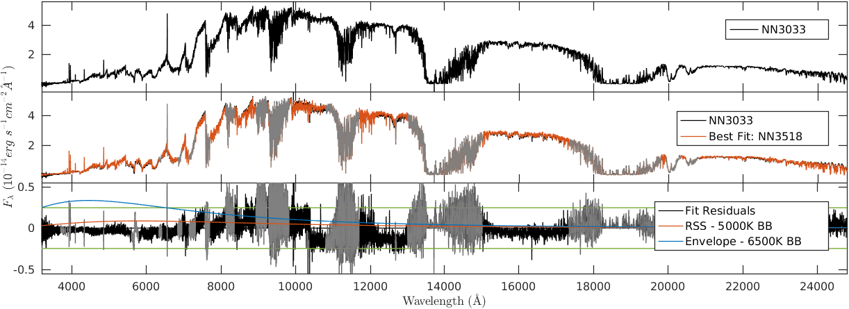
Figure 7.— NN3033

Figure 8.— NN3034

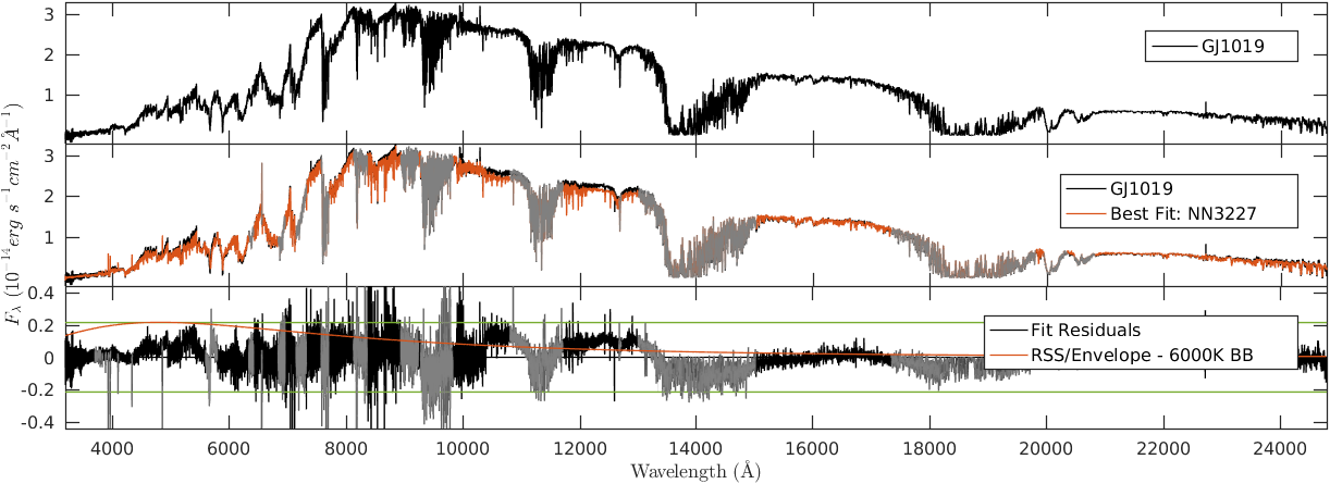
Figure 9.— GJ1019

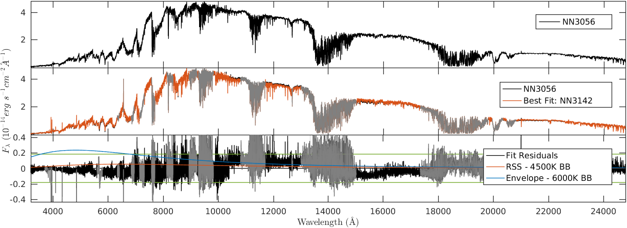
Figure 10.— NN3056

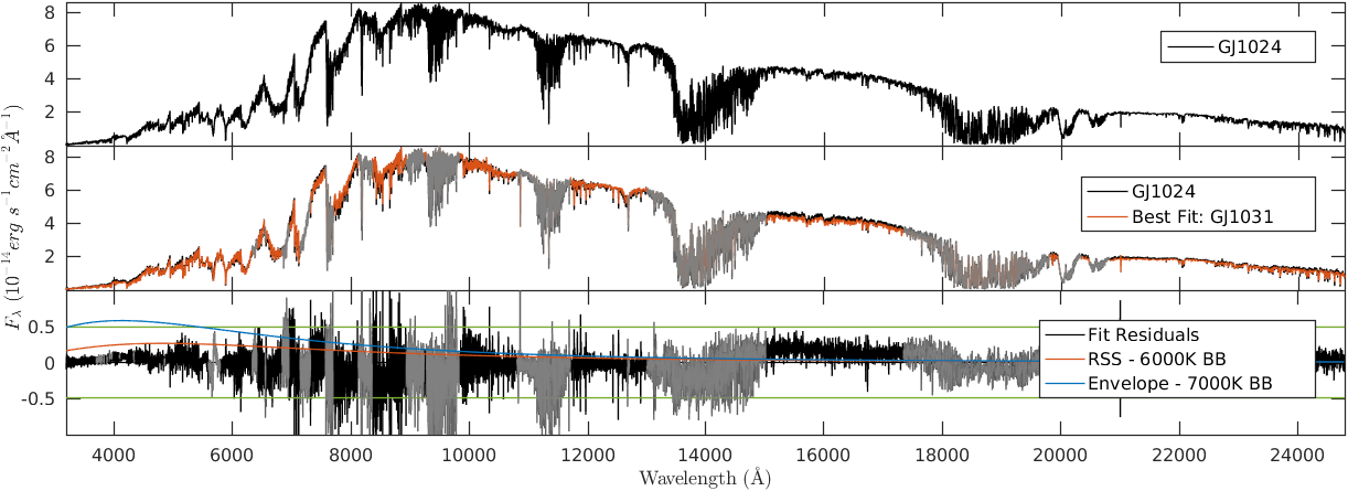
Figure 11.— GJ1024

Figure 12.— GJ1029

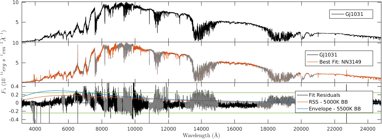
Figure 13.— GJ1031

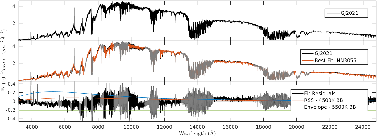
Figure 14.— GJ2021

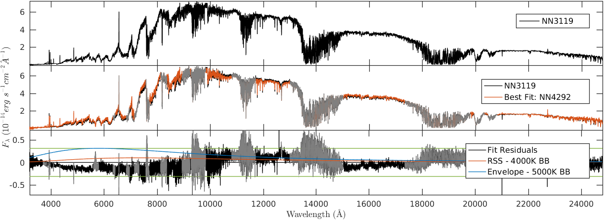
Figure 15.— NN3119

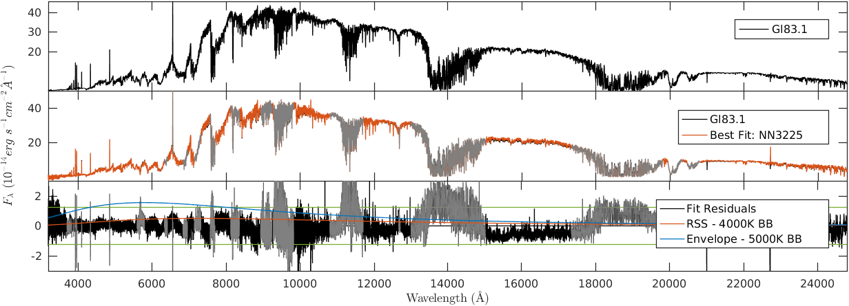
Figure 16.— Gl83.1

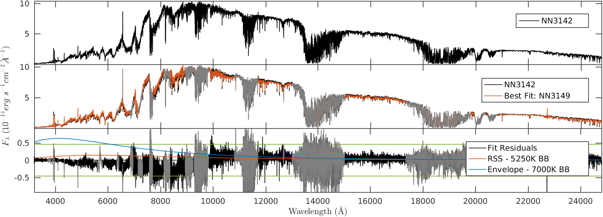
Figure 17.— NN3142

Figure 18.— NN3143

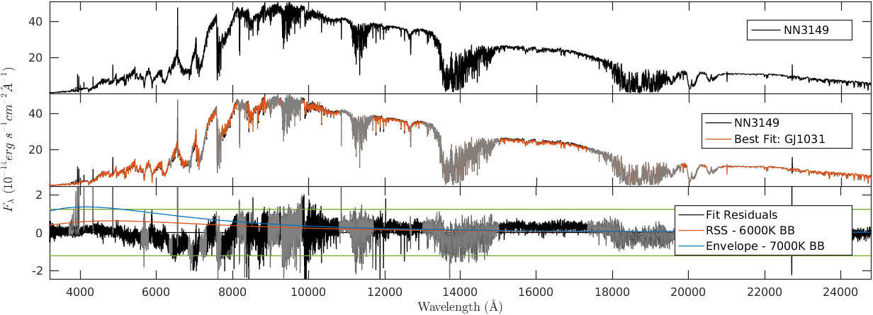
Figure 19.— NN3149

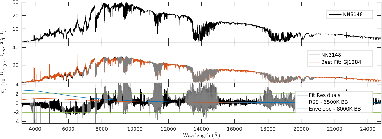
Figure 20.— NN3148

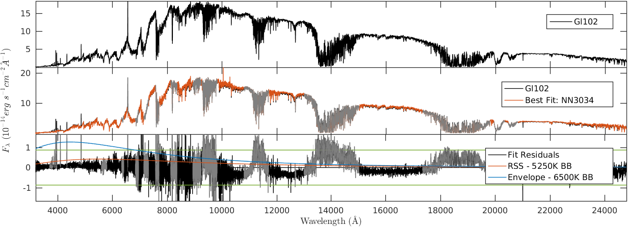
Figure 21.— Gl102

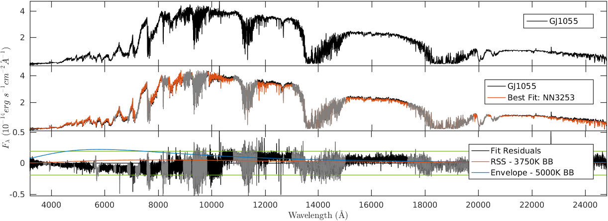
Figure 22.— GJ1055

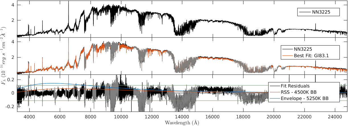
Figure 23.— NN3225

Figure 24.— NN3227

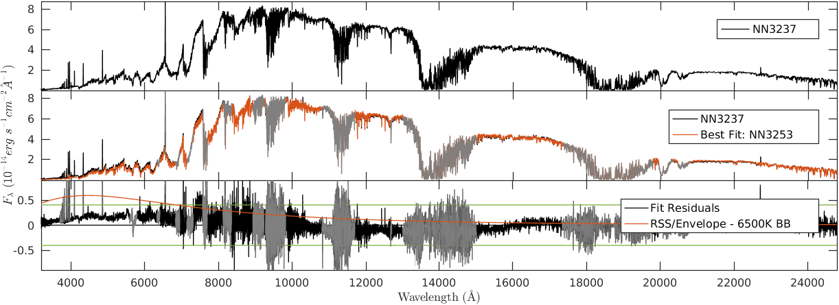
Figure 25.— NN3237

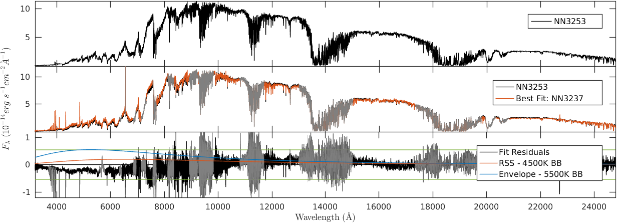
Figure 26.— NN3253

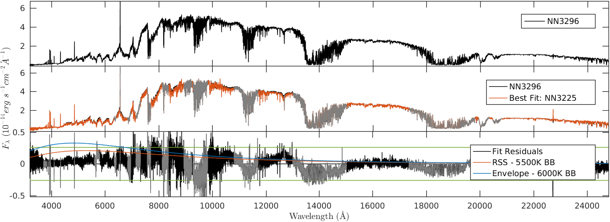
Figure 27.— NN3296

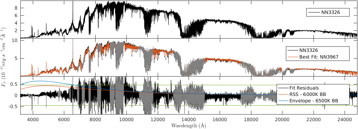
Figure 28.— NN3326

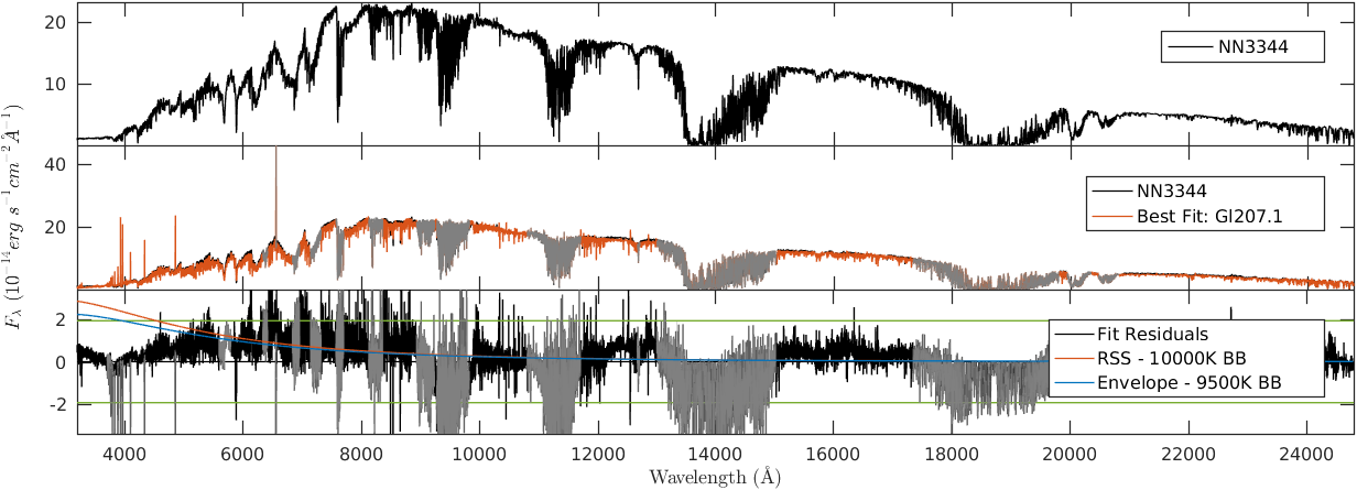
Figure 29.— NN3344

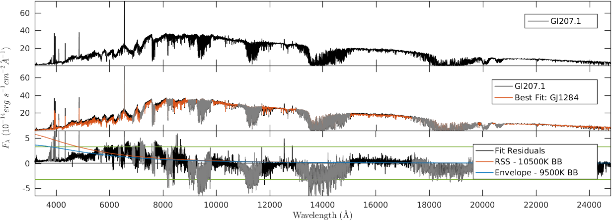
Figure 30.— Gl207.1

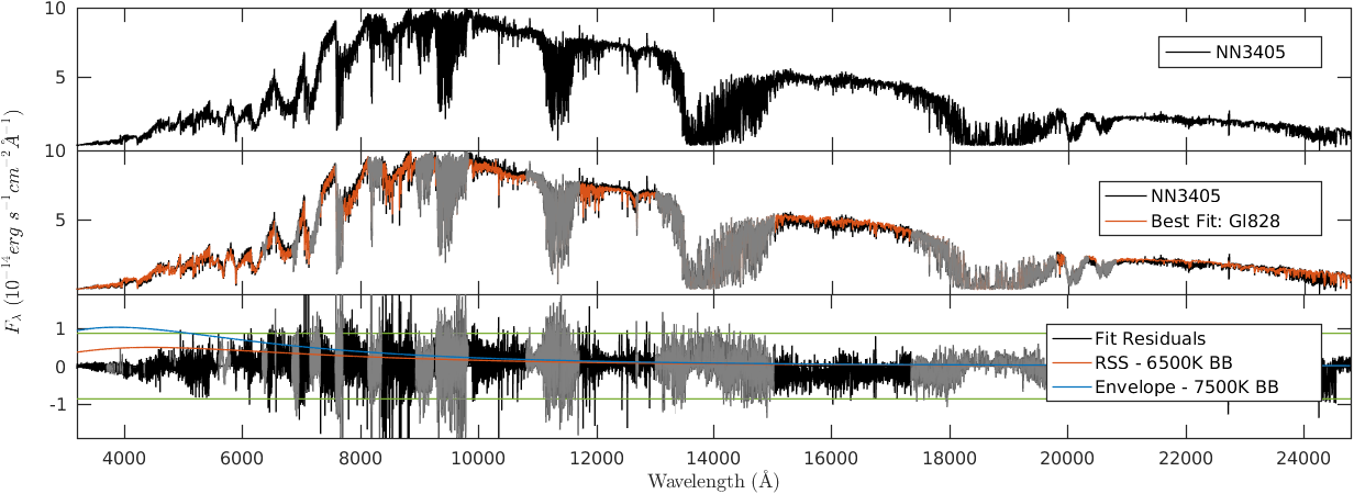
Figure 31.— NN3405

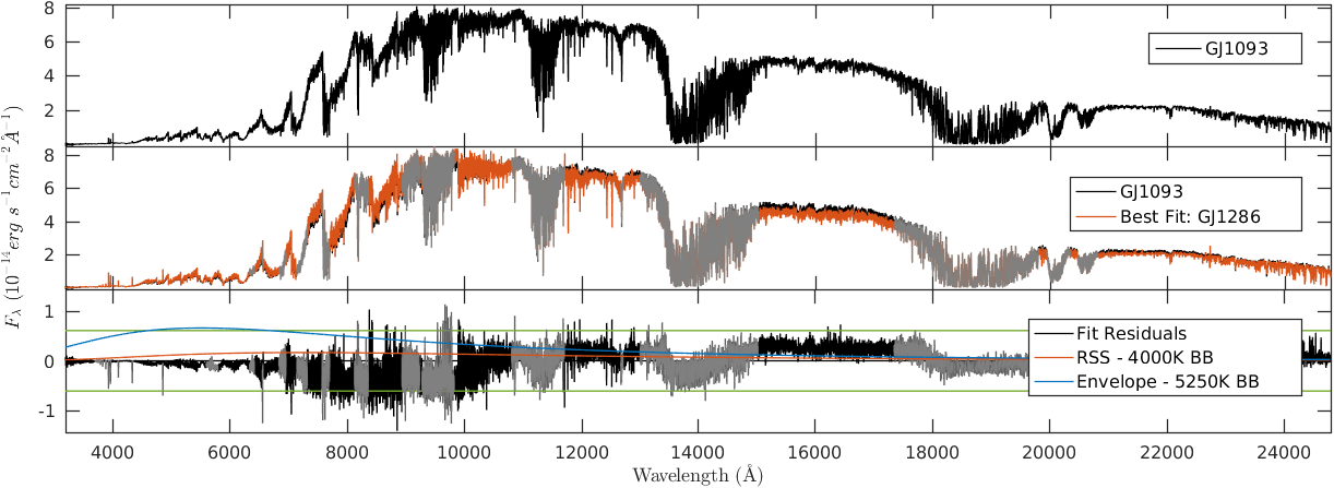
Figure 32.— GJ1093

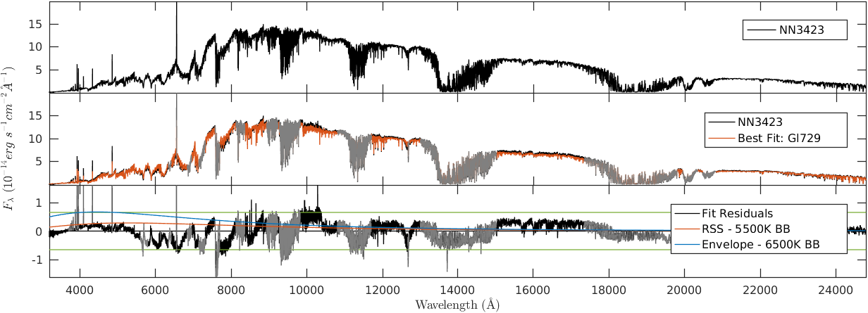
Figure 33.— NN3423

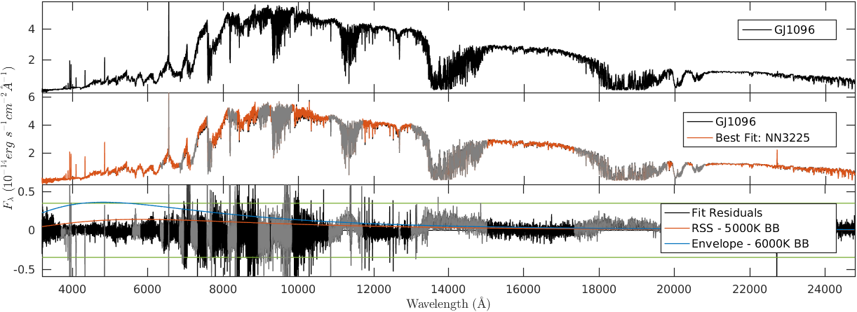
Figure 34.— GJ1096

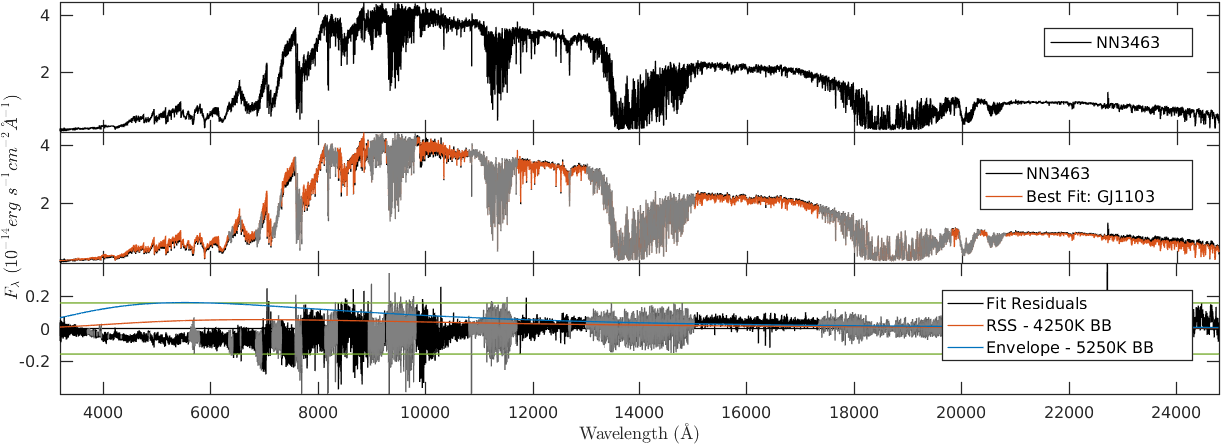
Figure 35.— NN3463

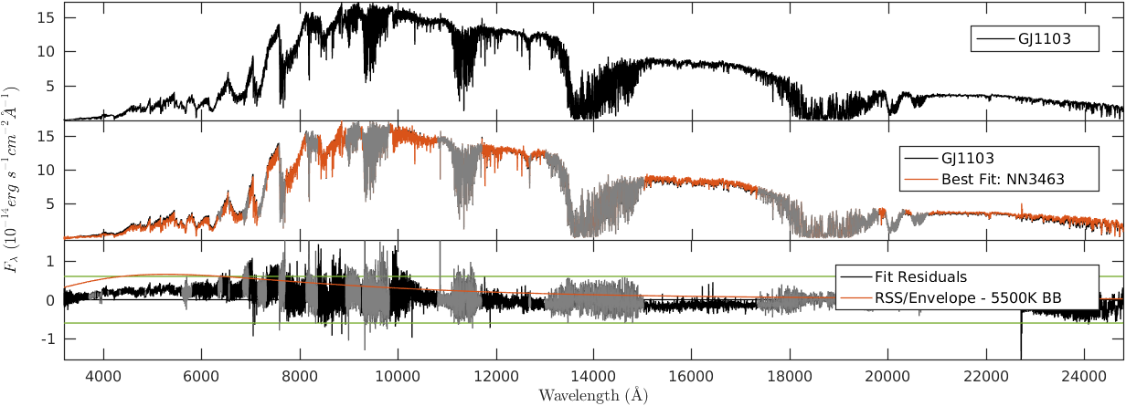
Figure 36.— GJ1103

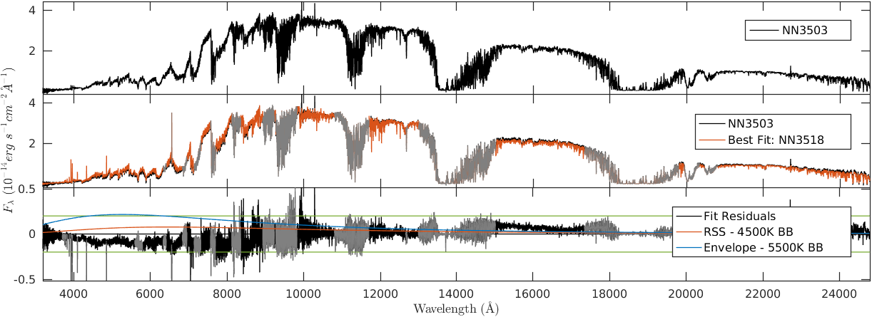
Figure 37.— NN3503

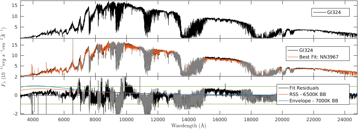
Figure 38.— Gl324

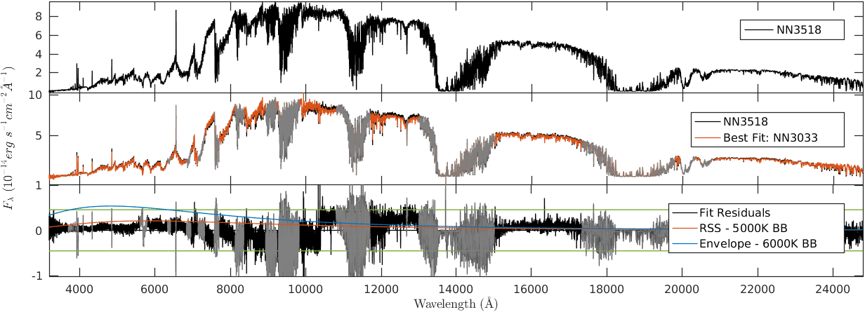
Figure 39.— NN3518

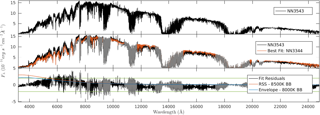
Figure 40.— NN3543

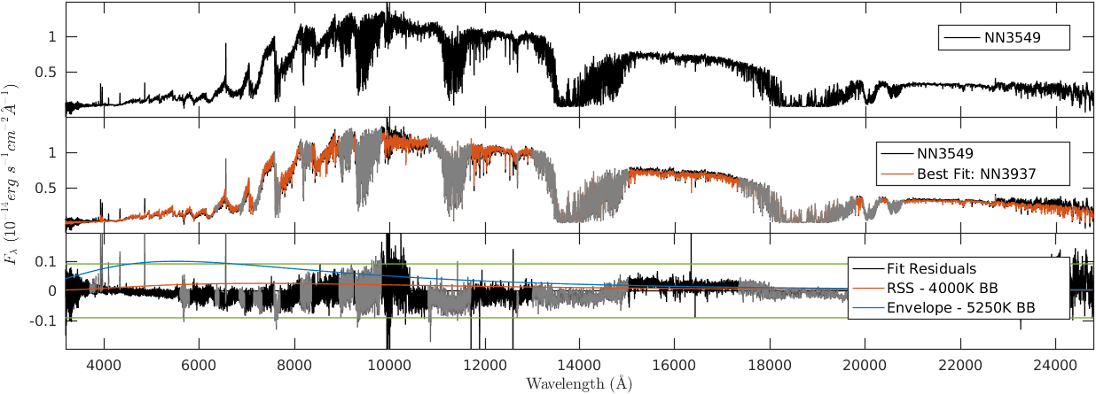
Figure 41.— NN3549

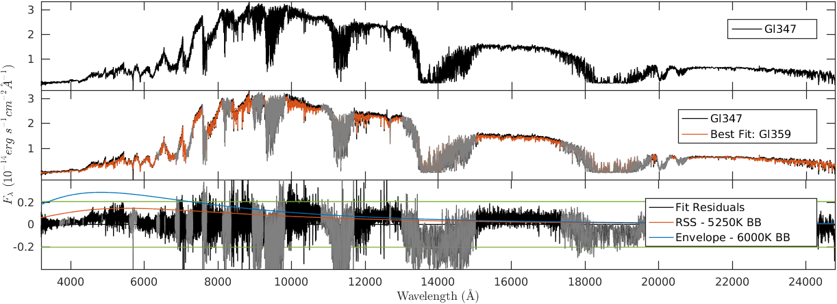
Figure 42.— Gl347

Figure 43.— Gl359

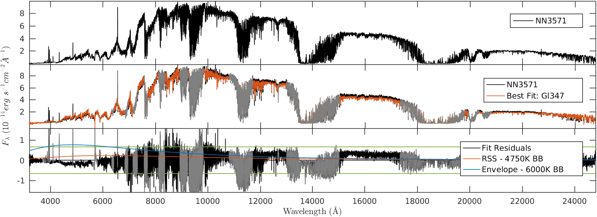
Figure 44.— NN3571

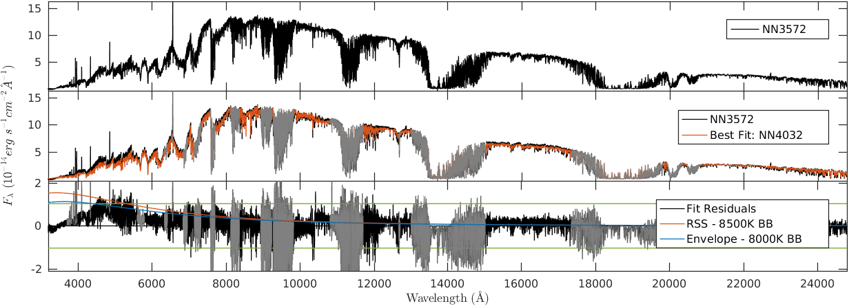
Figure 45.— NN3572

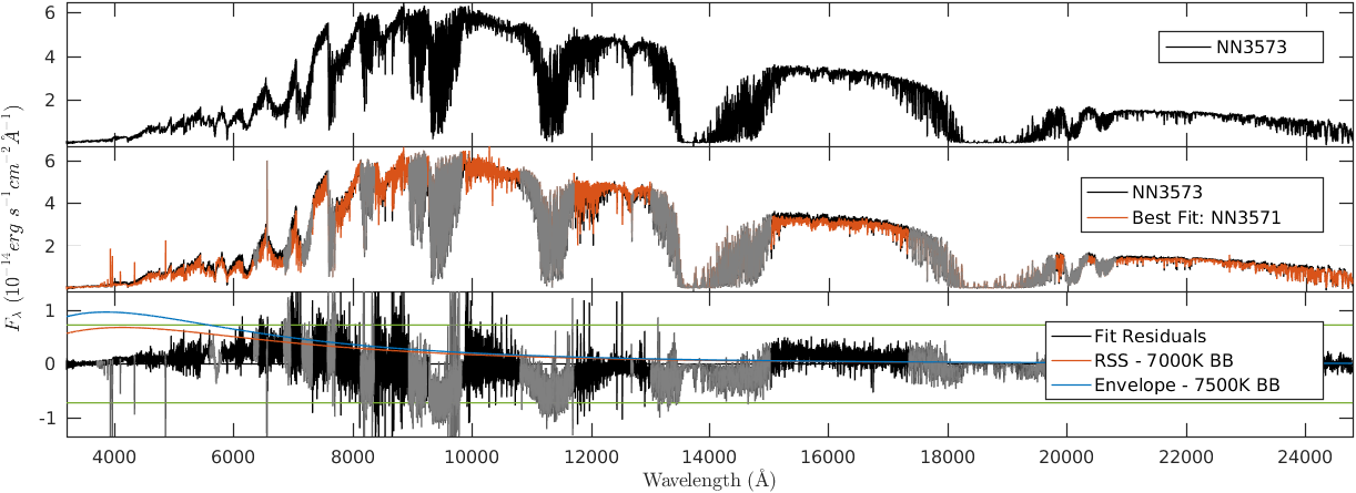
Figure 46.— NN3573

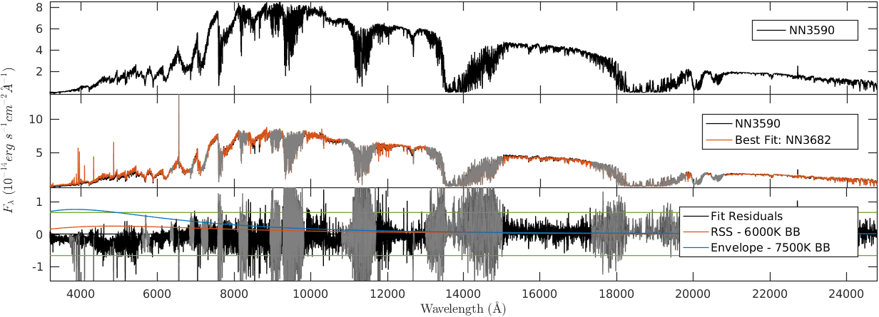
Figure 47.— NN3590

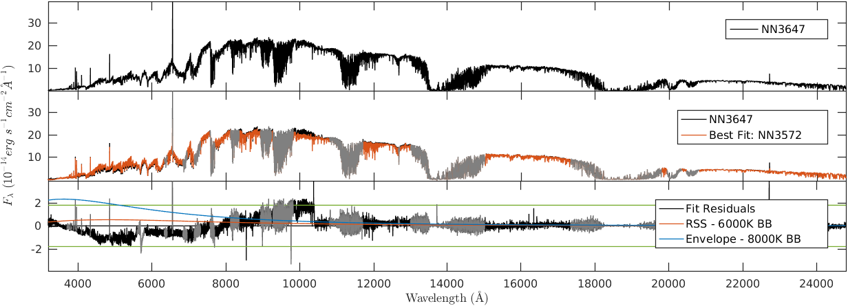
Figure 48.— NN3647

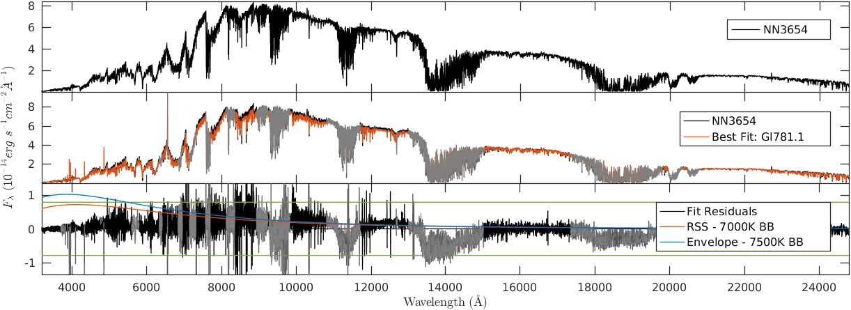
Figure 49.— NN3654

Figure 50.— NN3657

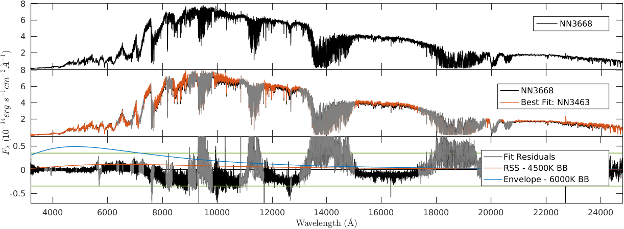
Figure 51.— NN3668

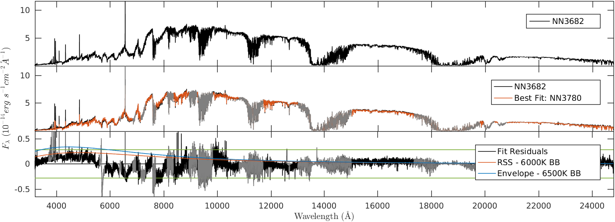
Figure 52.— NN3682

Figure 53.— NN3685

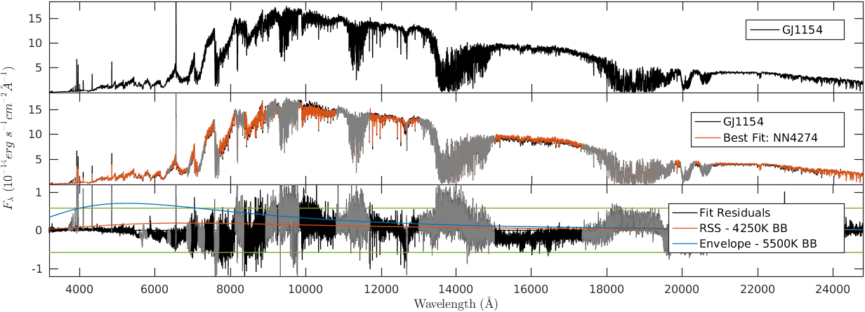
Figure 54.— GJ1154

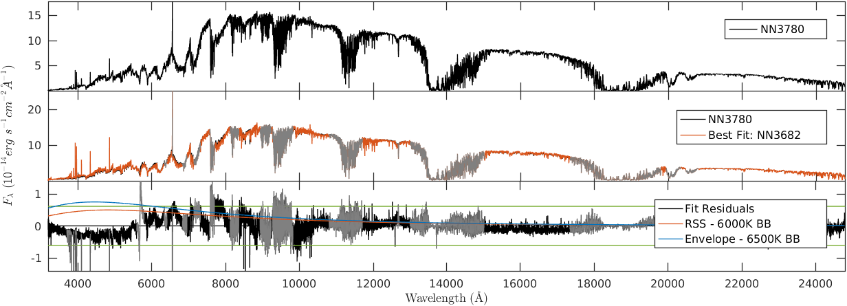
Figure 55.— NN3780

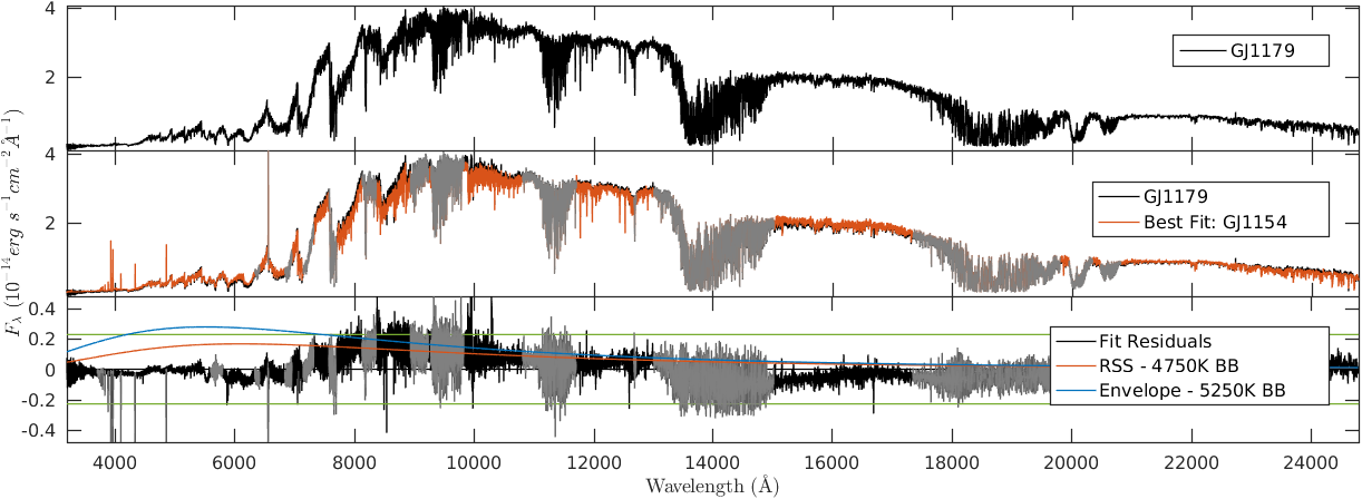
Figure 56.— GJ1179

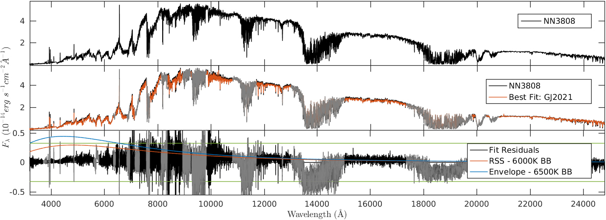
Figure 57.— NN3808

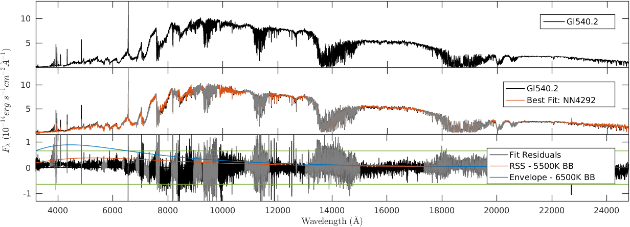
Figure 58.— Gl540.2

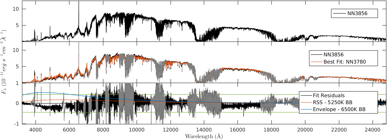
Figure 59.— NN3856

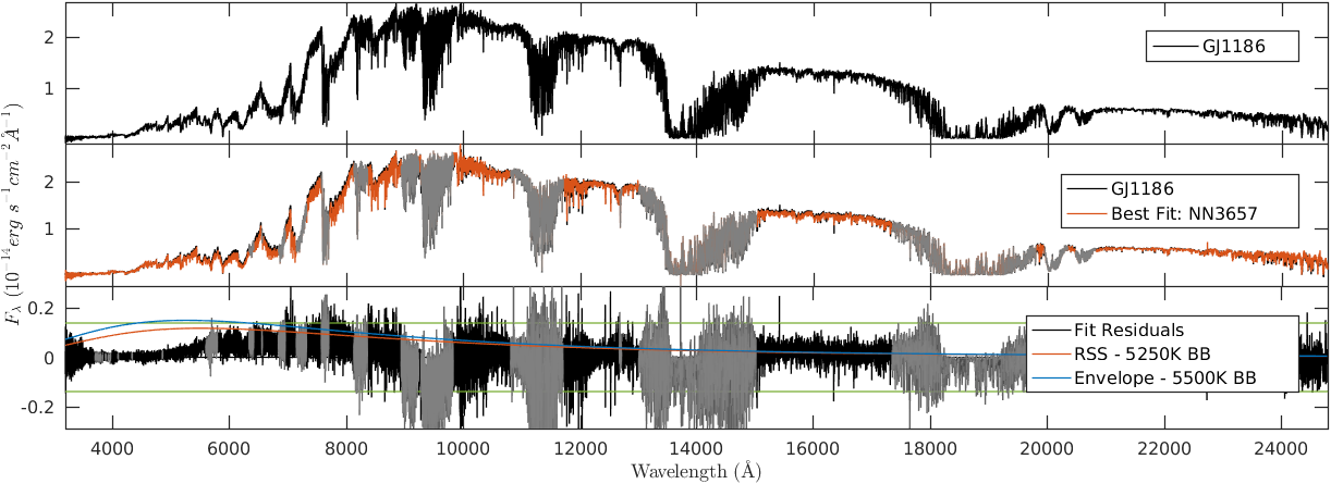
Figure 60.— GJ1186

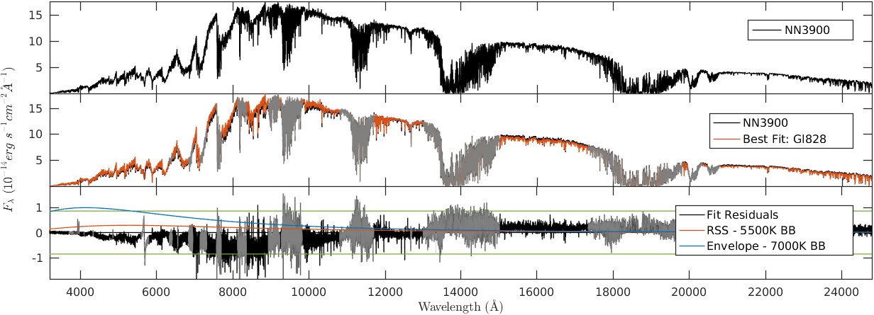
Figure 61.— NN3900

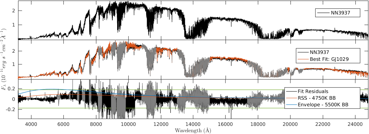
Figure 62.— NN3937

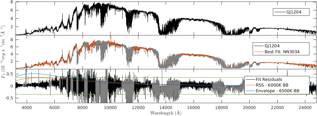
Figure 63.— GJ1204

Figure 64.— NN3967

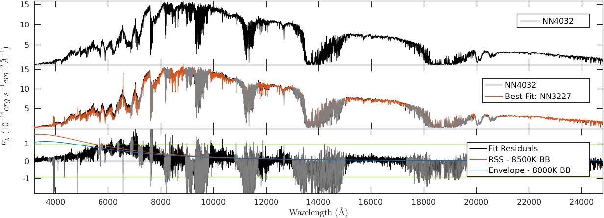
Figure 65.— NN4032

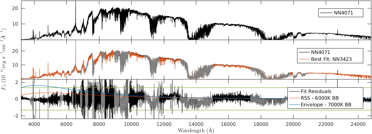
Figure 66.— NN4071

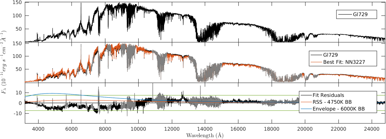
Figure 67.— Gl729

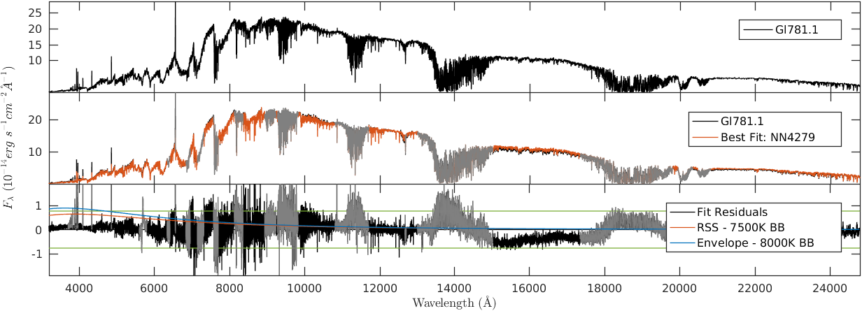
Figure 68.— Gl781.1

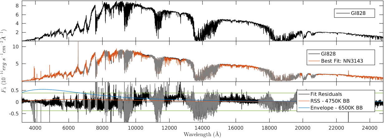
Figure 69.— Gl828

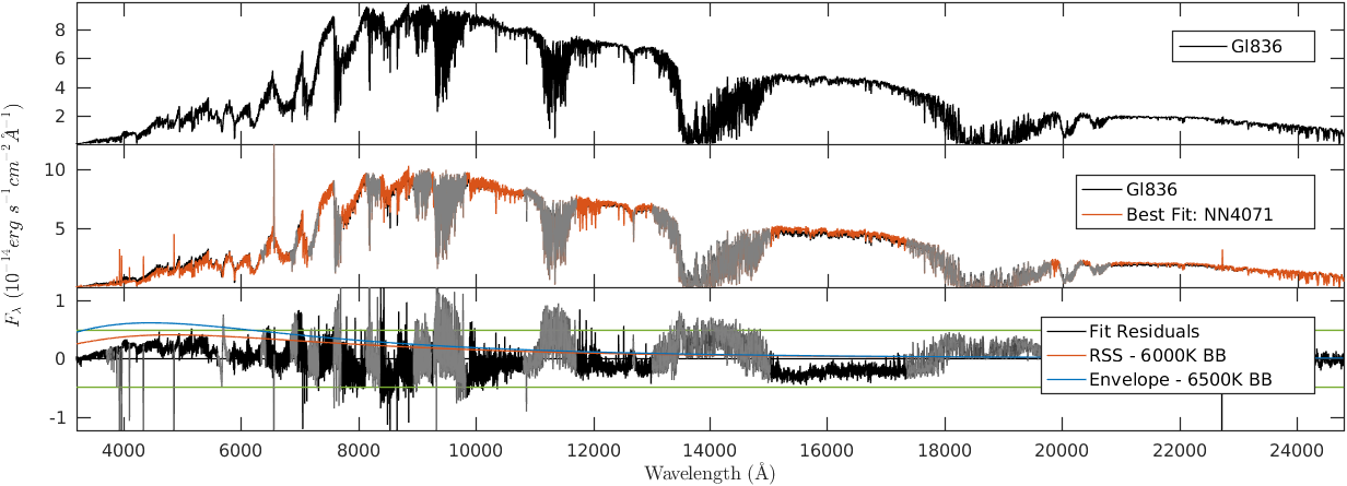
Figure 70.— Gl836

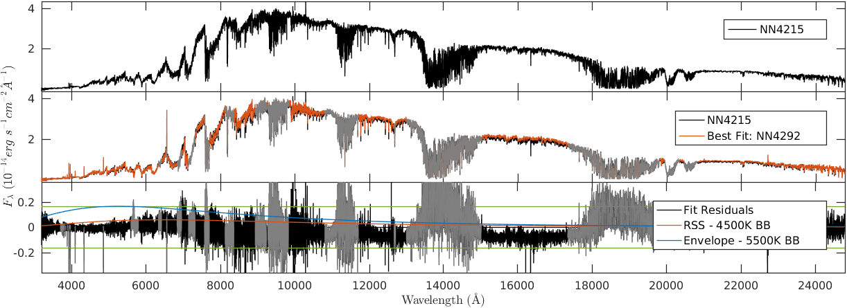
Figure 71.— NN4215

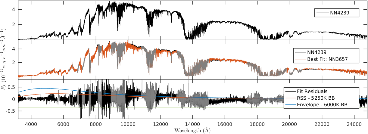
Figure 72.— NN4239

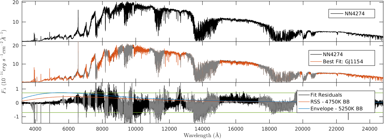
Figure 73.— NN4274

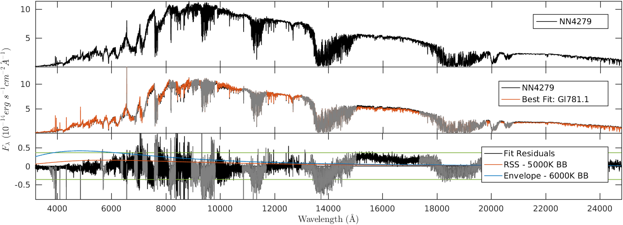
Figure 74.— NN4279

Figure 75.— NN4292

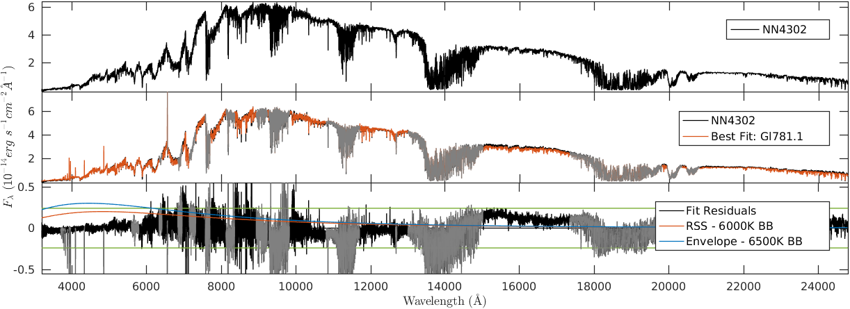
Figure 76.— NN4302

Figure 77.— GJ1284

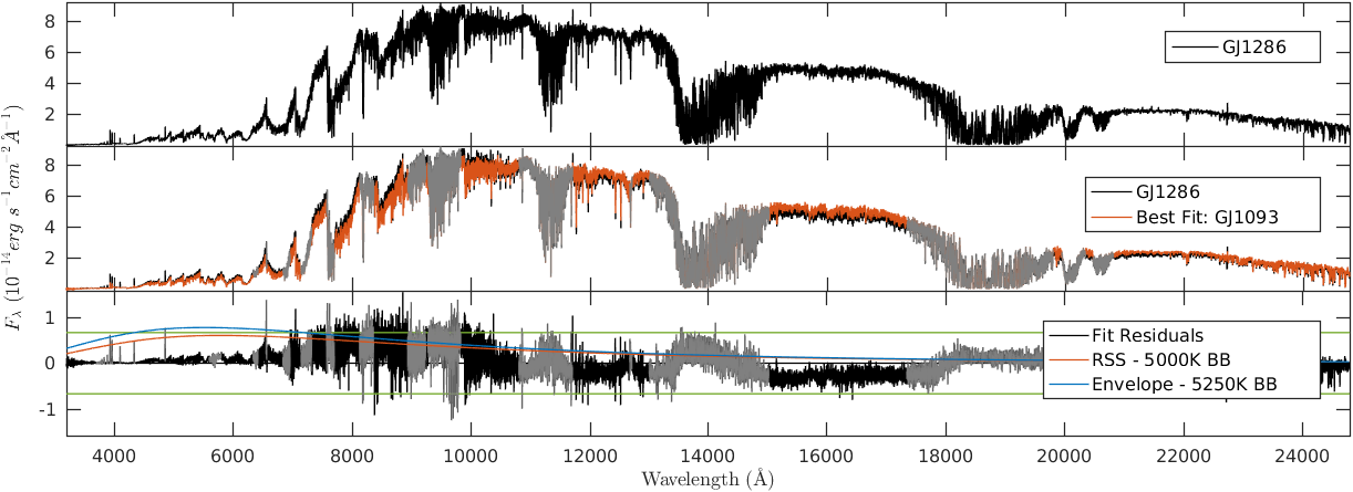
Figure 78.— GJ1286

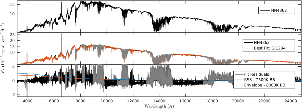
Figure 79.— NN4362

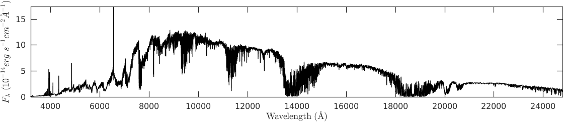
Figure 80.— NN3010

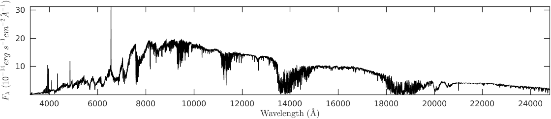
Figure 81.— NN3039

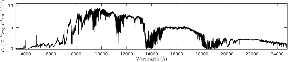
Figure 82.— NN3076

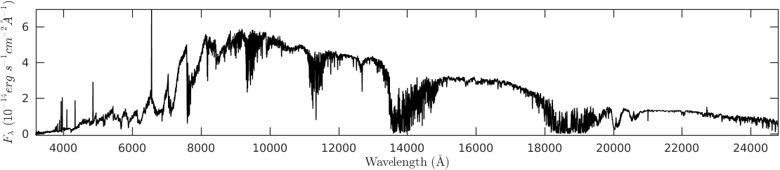
Figure 83.— NN3129

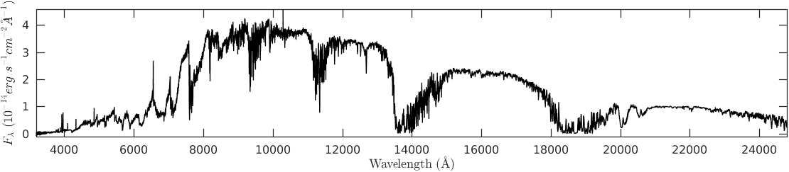
Figure 84.— NN3224

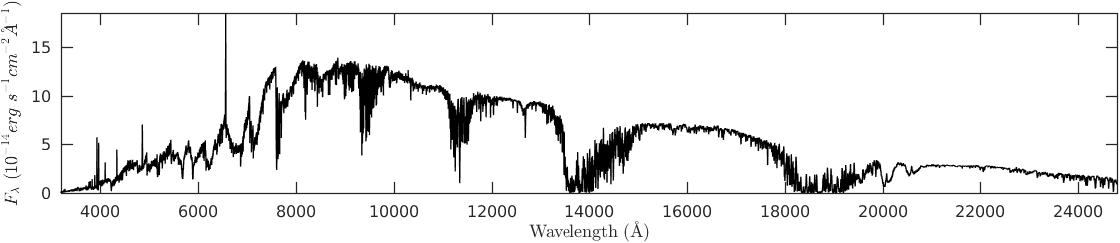
Figure 85.— NN3261

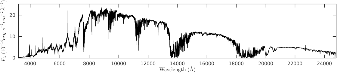
Figure 86.— NN3304

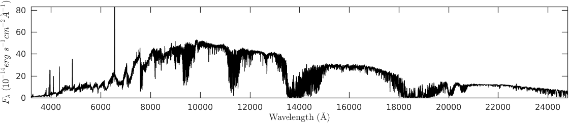
Figure 87.— NN3322

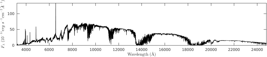
Figure 88.— NN3332

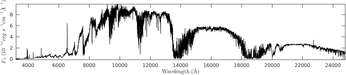
Figure 89.— GJ1083

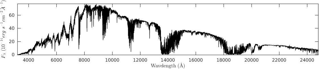
Figure 90.— Gl268.3

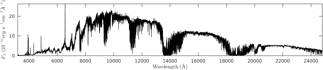
Figure 91.— NN3454

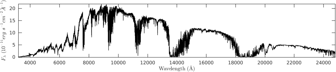
Figure 92.— NN3466

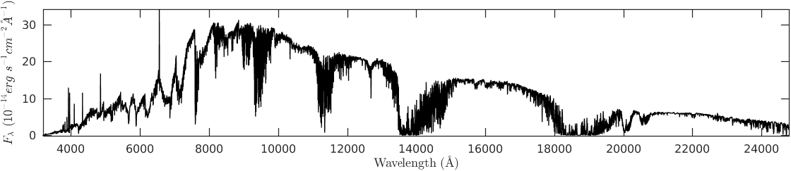
Figure 93.— GJ1108

Figure 94.— Gl300

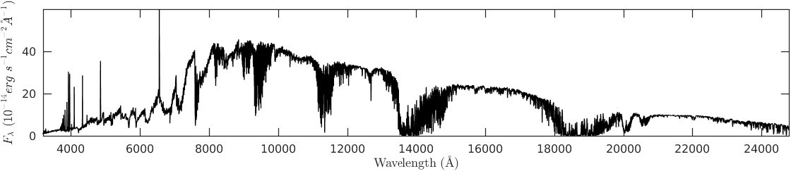
Figure 95.— GJ2069

Figure 96.— GJ1116

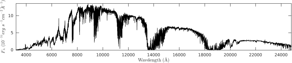
Figure 97.— NN3981

Figure 98.— GJ1210

Figure 99.— Gl791.2

Figure 100.— NN4201

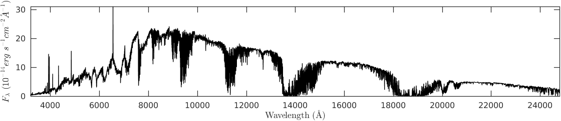
Figure 101.— NN4231

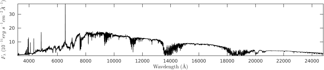
Figure 102.— NN4282

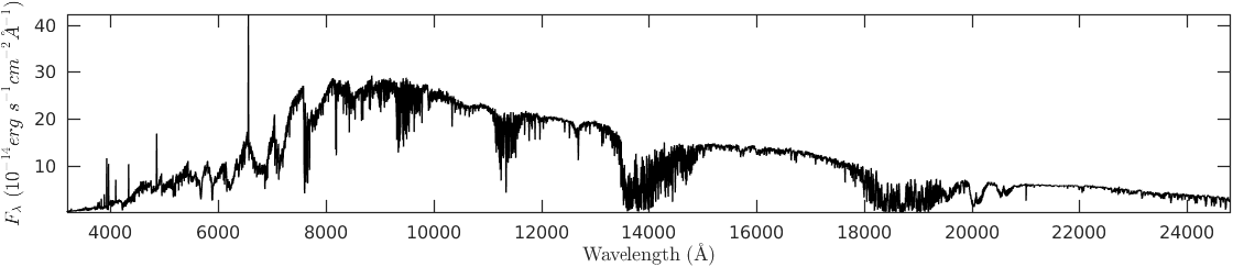
Figure 103.— NN4326

Figure 104.— NN4360

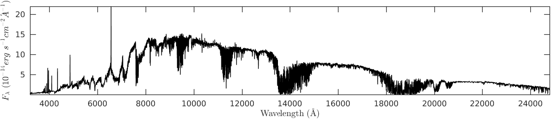
Figure 105.— NN4378

References

- Bergeron et al. (2001) Bergeron, P., Leggett, S. K., & Ruiz, M. T. 2001, ApJS, 133, 413
- Bergeron et al. (2011) Bergeron, P., Wesemael, F., Dufour, P., et al. 2011, ApJ, 737, 28
- Chen et al. (2014) Chen, Y.-P., Trager, S. C., Peletier, R. F., et al. 2014, A&A, 565, A117
- De Rosa et al. (2014) De Rosa, R. J., Patience, J., Wilson, P. A., et al. 2014, MNRAS, 437, 1216
- Dong et al. (2015) Dong, S., Katz, B., Kushnir, D., & Prieto, J. L. 2015, MNRAS, 454, L61
- Farihi et al. (2010) Farihi, J., Hoard, D. W., & Wachter, S. 2010, ApJS, 190, 275
- Ferrario (2012) Ferrario, L. 2012, MNRAS, 426, 2500
- Fontaine et al. (2001) Fontaine, G., Brassard, P., & Bergeron, P. 2001, PASP, 113, 409
- Freudling et al. (2013) Freudling, W., Romaniello, M., Bramich, D. M., et al. 2013, A&A, 559, A96
- García-Berro & Oswalt (2016) García-Berro, E., & Oswalt, T. D. 2016, New A Rev., 72, 1
- Giammichele et al. (2012) Giammichele, N., Bergeron, P., & Dufour, P. 2012, ApJS, 199, 29
- Gliese & Jahreiss (1995) Gliese, W., & Jahreiss, H. 1995, VizieR Online Data Catalog, 5070
- Holberg et al. (2002) Holberg, J. B., Oswalt, T. D., & Sion, E. M. 2002, ApJ, 571, 512
- Holberg & Bergeron (2006) Holberg, J. B., & Bergeron, P. 2006, AJ, 132, 1221
- Holberg et al. (2008) Holberg, J. B., Sion, E. M., Oswalt, T., et al. 2008, AJ, 135, 1225
- Horne (1986) Horne, K. 1986, PASP, 98, 609
- Howell (2011) Howell, D. A. 2011, Nature Communications, 2, 350
- Husser et al. (2013) Husser, T.-O., Wende-von Berg, S., Dreizler, S., et al. 2013, A&A, 553, A6
- Ivanova et al. (2013) Ivanova, N., Justham, S., Chen, X., et al. 2013, A&A Rev., 21, 59
- Jones & West (2016) Jones, D. O., & West, A. A. 2016, ApJ, 817, 1
- Katz & Dong (2012) Katz, B., & Dong, S. 2012, arXiv:1211.4584
- Katz et al. (2014) Katz, B., Dong, S., & Kushnir, D. 2014, arXiv:1402.7083
- Kepler et al. (2007) Kepler, S. O., Kleinman, S. J., Nitta, A., et al. 2007, MNRAS, 375, 1315
- Kleinman et al. (2013) Kleinman, S. J., Kepler, S. O., Koester, D., et al. 2013, ApJS, 204, 5
- Kowalski & Saumon (2006) Kowalski, P. M., & Saumon, D. 2006, ApJ, 651, L137
- Kushnir et al. (2013) Kushnir, D., Katz, B., Dong, S., Livne, E., & Fernández, R. 2013, ApJ, 778, L37
- Moehler et al. (2014) Moehler, S., Modigliani, A., Freudling, W., et al. 2014, A&A, 568, A9
- Maoz et al. (2014) Maoz, D., Mannucci, F., & Nelemans, G. 2014, ARA&A, 52, 107
- Martin et al. (2005) Martin, D. C., Fanson, J., Schiminovich, D., et al. 2005, ApJ, 619, L1
- Mason et al. (2009) Mason, B. D., Hartkopf, W. I., Gies, D. R., Henry, T. J., & Helsel, J. W. 2009, AJ, 137, 3358
- Mason et al. (2001) Mason, B. D., Wycoff, G. L., Hartkopf, W. I., Douglass, G. G., & Worley, C. E. 2001, AJ, 122, 3466
- Nugent et al. (2011) Nugent, P. E., Sullivan, M., Cenko, S. B., et al. 2011, Nature, 480, 344
- Oswalt et al. (2016) Oswalt, J. B. H. T. D., Sion, E. M., & McCook, G. P. 2016, arXiv:1606.01236
- Ofek (2014) Ofek, E. O. 2014, Astrophysics Source Code Library, ascl:1407.005
- Pickles (1998) Pickles, A. J. 1998, PASP, 110, 863
- Raghavan et al. (2010) Raghavan, D., McAlister, H. A., Henry, T. J., et al. 2010, ApJS, 190, 1
- Reid & Hawley (2005) Reid, I. N., & Hawley, S. L. 2005, New Light on Dark Stars Red Dwarfs, Low-Mass Stars, Brown Stars, by I.N. Reid and S.L. Hawley. Springer-Praxis books in astrophysics and astronomy. Praxis Publishing Ltd, 2005. ISBN 3-540-25124-3,
- Shkolnik et al. (2010) Shkolnik, E. L., Hebb, L., Liu, M. C., Reid, I. N., & Collier Cameron, A. 2010, ApJ, 716, 1522
- Skrutskie et al. (2006) Skrutskie, M. F., Cutri, R. M., Stiening, R., et al. 2006, AJ, 131, 1163
- Stauffer et al. (2010) Stauffer, J., Tanner, A. M., Bryden, G., et al. 2010, PASP, 122, 885
- Toonen & Nelemans (2013) Toonen, S., & Nelemans, G. 2013, A&A, 557, A87
- Tremblay et al. (2011) Tremblay, P.-E., Bergeron, P., & Gianninas, A. 2011, ApJ, 730, 128
- Vernet et al. (2011) Vernet, J., Dekker, H., D’Odorico, S., et al. 2011, A&A, 536, A105
- Wenger et al. (2000) Wenger, M., Ochsenbein, F., Egret, D., et al. 2000, A&AS, 143, 9
- West et al. (2004) West, A. A., Hawley, S. L., Walkowicz, L. M., et al. 2004, AJ, 128, 426
- Winget & van Horn (1987) Winget, D. E., & van Horn, H. M. 1987, IAU Colloq. 95: Second Conference on Faint Blue Stars, 363
- Yaron & Gal-Yam (2012) Yaron, O., & Gal-Yam, A. 2012, PASP, 124, 668