A quantum retrograde canon:
Complete population transfer in $n^{2}$-state systems

Abstract

We present a novel approach for analytically reducing a family of time-dependent multi-state quantum control problems to two-state systems. The presented method translates between $SU(2)\text{\texttimes}SU(2)$ related $n^{2}$-state systems and two-state systems, such that the former undergo complete population transfer (CPT) if and only if the latter reach specific states. For even $n$, the method translates any two-state CPT scheme to a family of CPT schemes in $n^{2}$-state systems. In particular, facilitating CPT in a four-state system via real time-dependent nearest-neighbors couplings is reduced to facilitating CPT in a two-level system. Furthermore, we show that the method can be used for operator control, and provide conditions for producing several universal gates for quantum computation as an example. In addition, we indicate a basis for utilizing the method in optimal control problems.

Multi-state quantum systems are in the frontier of quantum control research, holding high potential for reducing computation complexity (Lanyon et al., 2009), and strengthening communication security (Cerf et al., 2002) in quantum information technologies (Nielsen and Chuang, 2002). A central topic in multi-state control is complete population transfer (CPT), where a system is transferred between orthogonal states. This issue is a fundamental task in applications such as state preparation and entanglement transfer (Sørensen and Mølmer, 1999).

The simplest and most studied quantum control problems deal with two-state systems (Allen and Eberly, 1975),(Torosov and Vitanov, 2008). As we move to multiple states, synthesis and analysis of control schemes become increasingly difficult. Hence, multi-state control problems are often approached by some method of reduction to one or more two-state problems (Romano and D’Alessandro, 2016),(Genov et al., 2011). One such method is adiabatic elimination (Solá et al., 1999), in which the system’s dynamics are approximated by a two-state system through the elimination of irrelevant, non-resonantly coupled states. While this approach is often adequate, its applicability is conditioned on parameters’ range and its results may suffer significant inaccuracies under multiple eliminations (Paulisch et al., 2014). Another reduction method (Hioe, 1987) provides analytic solutions to $N$-level systems with $SU(2)$ dynamic symmetry in terms of the their fundamental two-state representation. While this approach is exact, it is limited to systems with $su(2)$ dynamical Lie algebra, and thus have only three degrees of freedom at each moment of time.

In this paper, we present the quantum retrograde canon, a novel method for analytically reducing time-dependent multi-state quantum control problems to two-state systems. The reduction method is based on an exact translation between two-state systems and time-dependent $n^{2}$-state Hamiltonians with $su(2)\oplus su(2)$ dynamical Lie algebra. The principle idea underlying the translation resembles the technique of the retrograde canon in music, where a musical line is played simultaneously with another copy of it, inverted in time (see “Crab Canon” by Bach (Bach, 1747)). Analogously, the quantum retrograde canon maps a one-qubit scheme to a two-qubit “retrograde canon” - taking one qubit through the dynamics of the original system and the other qubit through the same dynamics, inverted in time. Given an appropriate choice of basis, the two-qubit system undergoes CPT if and only if the one-qubit system reaches a specific state. Since the mapping is invertible, one can apply the method the other way around and translate two-qubit schemes, which have six degrees of freedom at each moment, to two-state schemes, which have only three degrees of freedom at each moment. By using higher order representation of the two-qubit system, and an appropriate choice of basis, one gets a translation method between two-state schemes and $SU(2)\text{\texttimes}SU(2)$ controlled $n^{2}$-state CPT schemes. In particular, for even $n$, the method translates any two-state CPT scheme to CPT schemes in $n^{2}$-state systems.

The paper is structured as follows: In section I, we define the retrograde canon. In section II, we illustrate a way in which the retrograde canon reduces four-level CPT problems to two-level CPT problems. In section III, we formulate and prove the fundamental observation underlying the reduction method. In section IV, we state a more general claim regarding four-level CPT problems. In section V, we discuss two concrete examples of the method’s application. In section VI, we indicate the use of the method for optimal and operator control problems. Lastly, in section VII, we consider generalizations of the method, including application to $n^{2}$-state systems through higher order representations of the $SU(2)$ group. In section VIII, we summarize. Various technical issues are discussed in the appendices.

I basic definitions

We begin with defining the key notions of the retrograde canon. Let $H(t)$ be a time-dependent two state system Hamiltonian and $U(t)$ be the propagator generated by $H$, i.e., $U$ is the solution of Schrödinger’s operator equation $\dot{U}(t)=-iH(t)U(t)$ with the initial condition $U(0)=I_{2}$. We define the Retrograde of $H$, starting from time $T$> 0, by

$$H^{R}(t)\equiv-H(T-t)$$ (1)

It can be verified by differentiation that $U^{R},$ the propagator generated by $H^{R}$, satisfies:

$$U^{R}(t)=U(T-t)U(T)^{-1}$$ (2)

$U^{R}(t)$ takes states backwards in time along the path they trace when acted on by $U(t)$. That is, suppose that $|f\text{\textrangle}\equiv U(T)|i\text{\textrangle}$ - i.e., $|f\text{\textrangle}$ is the state to which the initial state $|i\text{\textrangle}$ evolves to in the original system - then

$$U^{R}(t)|f\text{\textrangle}=U(T-t)|i\text{\textrangle}$$ (3)

In what follows we will be interested in the the effect of acting simultaneously with both the original Hamiltonian and its retrograde. Thus, we define the Retrograde canon Hamiltonian, $H^{RC}$, by

$$H^{RC}(t)\equiv H^{R}(t)\text{$\otimes$$I_{2}+I_{2}\otimes H(t)$}$$ (4)

$H^{RC}$ acts on one qubit with the original time-dependent Hamiltonian, and on another qubit with its retrograde, starting from time $T>0$. clearly, $U^{RC}$, the Retrograde Canon Propagator generated by $H^{RC}$, satisfies:

$$U^{RC}(t)=U^{R}(t)\otimes U(t)$$ (5)

The retrograde canon is a one-to-one mapping from a $su(2)$ two-state time-dependent Hamiltonian in the time interval $[0,\,T]$ and a $su(2)\oplus su(2)$ four-state time-dependent Hamiltonian in the time interval $[0,\>T/2]$. Accordingly, any time-dependent four-state Hamiltonian of the form $\tilde{H}(t)=H^{b}(t)\text{$\otimes$$I_{2}+I_{2}\otimes H^{a}(t)$}$, where $H^{b}(t),H^{a}(t)$ are two-state Hamiltonians defined for $t\in[0,\>T/2]$, can be regarded as the retrograde canon of a unique two-state Hamiltonian, $H$, defined for $t\in[0,T]$ through

$$H(t)=\begin{cases}H^{a}(t)&0\leq t\leq T/2\\ -H^{b}(T-t)&T/2\leq t\leq T\end{cases}$$ (6)

Thus, the 6 degrees of freedom of the four-level momentary Hamiltonian $\tilde{H}(s)$ are mapped to 3+3 degrees of freedom of the two two-level momentary Hamiltonians, $H(s)$ and $H(T-s)$.

II AN APPLICATION OF THE METHOD

Let’s present a relatively general case of reducing CPT problems from four-state systems to two-state systems through the retrograde canon. This is not the most general four-level application of the method, but it is general enough to understand the idea. Consider the following four-level Hamiltonian:

$$\mathcal{H}(t)=\begin{pmatrix}0&A(t)&iE(t)&D(t)\\ A(t)&0&B(t)&iF(t)\\ -iE(t)&B(t)&0&C(t)\\ D(t)&-iF(t)&C(t)&0\end{pmatrix}$$ (7)

where $A(t),...,F(t)$ are six arbitrary real functions of time. Suppose we are interested in the conditions under which $\mathcal{H}(t)$ facilitates CPT from $\Psi_{1}=(1,0,0,0)^{\intercal}$ to $\Psi_{3}=(0,0,1,0)^{\intercal}$ at some time $\tau>0$, i.e., the conditions under which $1=|\text{\textlangle}\Psi_{3},\mathcal{U}(\tau)\Psi_{1}\text{\textrangle}|$, where $\mathcal{U}(t)$ is the propagator generated by $\mathcal{H}(t)$. Special cases of this problem are encountered in the literature (Solá et al., 1999)(Suchowski et al., 2011)(Svetitsky et al., 2014) and in applications. We will show that the through the retrograde canon we reduce this question to the question whether $e_{1}=(1,0)^{\intercal}$ evolves to $\pm e_{2}=\pm(0,1)^{\intercal}$ at time $T=2\tau$ in a two-state system governed by the Hamiltonian $H(t)=x(t)\sigma_{x}+y(t)\sigma_{y}+z(t)\sigma_{z}$, i.e.,

$$H(t)=\begin{pmatrix}z(t)&x(t)+iy(t)\\ x(t)-iy(t)&-z(t)\end{pmatrix}$$ (8)

where

$$\begin{array}[]{c}x(t)\equiv-\frac{1}{2}\begin{cases}C(t)-A(t)&0\leq t\leq T/2\\ C(T-t)+A(T-t)&T/2\leq t\leq T\end{cases}\\ y(t)\equiv\frac{1}{2}\begin{cases}E(t)+F(t)&0\leq t\leq T/2\\ E(T-t)-F(T-t)&T/2\leq t\leq T\end{cases}\\ z(t)\equiv\frac{1}{2}\begin{cases}B(t)+D(t)&0\leq t\leq T/2\\ B(T-t)-D(T-t)&T/2\leq t\leq T\end{cases}\end{array}$$

The translation between the two-level Hamiltonian of eq. 8 and the four-level Hamiltonian of eq. 7 is done in two stages, illustrated schematically in Figure 1: In the first stage, we change basis and define $\tilde{H}(t)\equiv W^{\text{\textdagger}}\mathcal{H}(t)W$, where

$$W\equiv\frac{1}{\sqrt{2}}\begin{pmatrix}1&0&0&1\\ 0&1&-1&0\\ 0&1&1&0\\ 1&0&0&-1\end{pmatrix}$$ (9)

In the second stage, we apply eq. 6 to $\tilde{H}(t)$ and get the two-level $H(t)$. That is, we consider $\tilde{H}(t)$ as the retrograde canon Hamiltonian of some $H(t)$, and solve for $H(t)$.

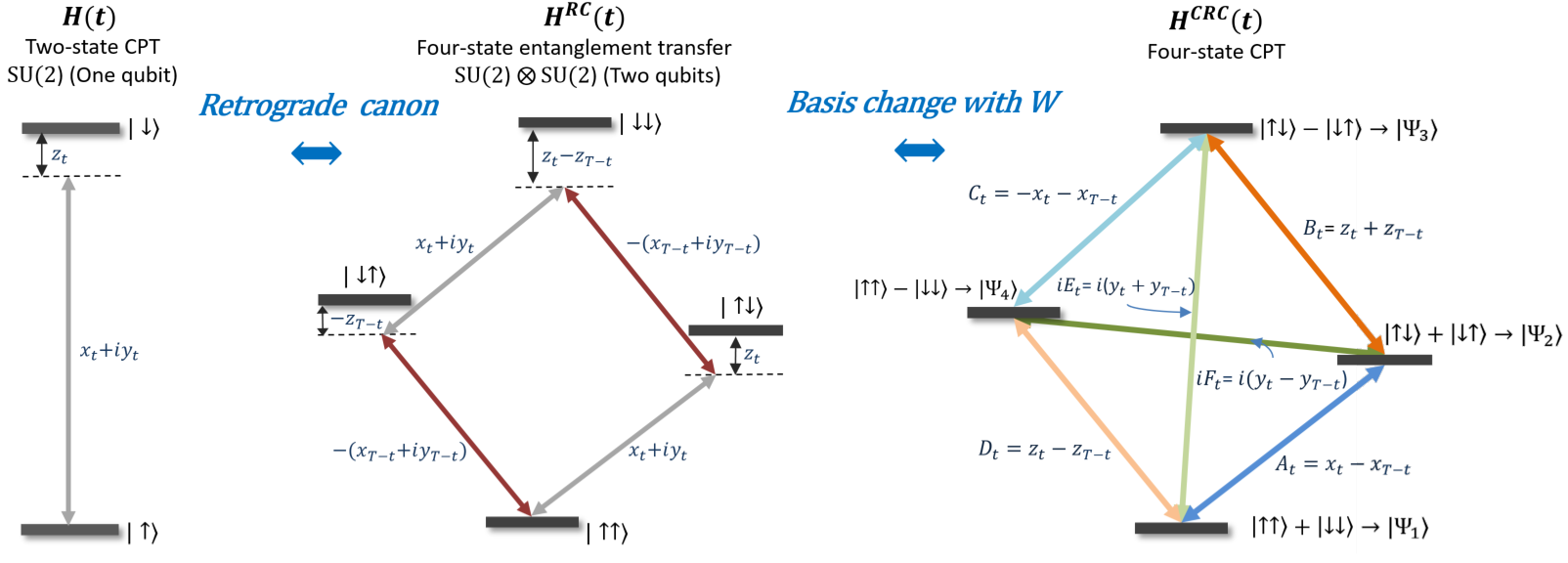
Figure 1: Couplings diagrams illustrating the translation method - Going opposite to the direction of the main text, we start from the two-state system (on the left, with lower indices indicating time). Applying the retrograde canon, defined in eq. 4, we get a four-state system of two independent qubits (in the middle). Switching basis using the unitary matrix $W$ defined in eq. 9, provides a four-state Hamiltonian of the form given in eq. 7 (on the right). We show below that the right system undergoes CPT at time $\tau$ if and only if the left system evolves from $|\downarrow\rangle$ to $\pm|\downarrow\rangle$ at time $2\tau$.

The claim that $\mathcal{H}(t)$ facilitates CPT from $\Psi_{1}=(1,0,0,0)^{\intercal}$ to $\Psi_{3}=(0,0,1,0)^{\intercal}$ at time $\tau$ if and only if $H(t)$ takes $e_{1}=(1,0)^{\intercal}$ to $\pm e_{2}=\pm(0,1)^{\intercal}$ at time $T=2\tau$ is a special case of the claim we formulate and prove below.

III the central observation

Prior to formulating the general claim for the case of four-state systems, from which the example above follows as a a special case, let us state and prove the observation which provides the basis for using the retrograde canon to reduce multi-state CPT problems to two-state systems:

$$U(T)|\uparrow\rangle=|\downarrow\rangle\Leftrightarrow U^{RC}(\tau)(|\downarrow\downarrow\rangle+|\uparrow\uparrow\rangle)=|\uparrow\downarrow\rangle-|\downarrow\uparrow\rangle$$ (10)

where $|\uparrow\rangle\equiv(1,0)^{\intercal}$ and $|\downarrow\rangle\equiv e^{i\alpha}(0,1)^{\intercal}$ for some $\alpha\in[0,2\pi)$. Eq. 10 states that a two-state Hamiltonian, $H$, facilitates CPT at time $T$ if and only if $H^{RC}$, facilitates a specific ’entanglement transfer’ at time $\tau\equiv T/2$. We emphasize that the path of $U(t)$ up to the point $t=T$ can be completely arbitrary. In particular, $U(\tau)$, which appears in $U^{RC}(\tau)=U(\tau)\otimes U^{R}(\tau)$, can be any $SU(2)$ matrix.

To prove the $\Rightarrow$ direction of eq. 10 we first note that eq. 3 tells us that for $\tau=T/2$,

$$U^{R}(\tau)|f\text{\textrangle}=U(\tau)|i\text{\textrangle}$$ (11)

Now, assume that indeed $U(T)|\uparrow\rangle=|\downarrow\rangle$. Since $U(\tau)$ is unitary, it transfers orthogonal states to orthogonal states. Thus, it is sensible to mark $U(\tau)|\uparrow\rangle\equiv|\tilde{\uparrow}\rangle$ and $U(\tau)|\downarrow\rangle\equiv|\tilde{\downarrow}\rangle$. From eq. 11 we get that $U^{R}(\tau)|\downarrow\rangle\text{=|$\tilde{\uparrow}\rangle$}$. Moreover, from the fact that $U(T)^{-1}$ is a $\pi$-rotation in a spin-half representation, and hence $U(T)^{-1}U(T)^{-1}=-I_{2}$, it follows that (marking $U_{t}\equiv U(t)$)

$$\begin{array}[]{c}U^{R}(\tau)|\uparrow\rangle=U_{\tau}U_{T}^{-1}|\uparrow\rangle\text{$=U_{\tau}U_{T}U_{T}^{-1}U_{T}^{-1}|\uparrow\rangle$}\\ =-U_{\tau}U_{T}|\uparrow\text{$\rangle$=$-U_{\tau}|\downarrow\rangle$}\end{array}$$ (12)

and therefore $U^{R}(\tau)|\uparrow\rangle=-|\tilde{\downarrow}\rangle$ . Hence,

$$\begin{array}[]{c}U^{RC}(\tau)(|\downarrow\downarrow\rangle+|\uparrow\uparrow\rangle)=\\ =U_{\tau}^{R}|\downarrow\rangle\otimes U_{\tau}|\downarrow\rangle+U_{\tau}^{R}|\uparrow\rangle\otimes U_{\tau}|\uparrow\rangle\\ =|\tilde{\uparrow}\tilde{\downarrow}\rangle-|\tilde{\downarrow}\tilde{\uparrow}\rangle=|\uparrow\downarrow\rangle-|\downarrow\uparrow\rangle\end{array}$$ (13)

where the last step follows from the Clebsh-Jordan fact that $|\uparrow\downarrow\rangle-|\downarrow\uparrow\rangle$ is a $SU(2)$ scalar.

To prove the $\Leftarrow$ direction of eq. 10 we utilize a slightly different perspective, which will also be useful for the generalizations of the retrograde canon presented below. We assume that $U^{RC}(\tau)(|\downarrow\downarrow\rangle+|\uparrow\uparrow\rangle)=|\uparrow\downarrow\rangle-|\downarrow\uparrow\rangle$ and need to prove that $U(T)|\uparrow\rangle=|\downarrow\rangle$. For the proof we shall use two simple facts: the first is that for any three 2-by-2 matrices, $A,\,B,\,m$,

$$(A\otimes B)F(m)=F(AmB^{\intercal})$$ (14)

where $F$ simply flattens matrices, i.e., $F\left(\begin{pmatrix}a&b\\ c&d\end{pmatrix}\right)=(a,b,c,d)^{\intercal}.$ Eq. 14 may be verified by direct calculation. The second, is that for $Y\equiv e^{+i\frac{\pi}{2}\sigma_{y}}=\begin{pmatrix}0&1\\ -1&0\end{pmatrix}$ ($\sigma_{i}$ are the Pauli matrices) and any $u\in SU(2)$,

$$uYu^{\intercal}=Y$$ (15)

Eq. 15 is in fact equivalent to the claim that $|\downarrow\uparrow\rangle-|\uparrow\downarrow\rangle$ is a $SU(2)$ scalar - the equivalence can be seen through eq. 14 and the observation that $|\uparrow\downarrow\rangle-|\downarrow\uparrow\rangle\rightarrow e^{i\alpha}F(Y)$ in the basis $\{|\uparrow\uparrow\rangle,|\uparrow\uparrow\rangle,|\uparrow\uparrow\rangle,|\uparrow\uparrow\rangle\}$ .

To proceed, we define $R\equiv e^{-i\alpha\sigma_{z}}$ and note that in the above basis $|\downarrow\downarrow\rangle+|\uparrow\uparrow\rangle\rightarrow F\left(\begin{pmatrix}1&0\\ 0&e^{2i\alpha}\end{pmatrix}\right)=e^{i\alpha}F(R)$. Now, it follows that the assumption is equivalent to

$$\begin{array}[]{c}Y=F^{-1}((U_{\tau}^{R}\otimes U_{\tau})F(R))=U_{\tau}^{R}RU_{\tau}^{\intercal}=\\ =U_{\tau}^{R}RY^{-1}U_{\tau}^{-1}U_{\tau}YU_{\tau}^{\intercal}=U_{\tau}^{R}RY^{-1}U_{\tau}^{-1}Y\end{array}$$ (16)

where we used eq. 14 in the second equality, inserted $I_{2}=Y^{-1}U_{\tau}^{-1}U_{\tau}Y$ in the third equality, and used eq. 15 in the fourth equality. Multiplying eq. 16 by $Y^{-1}$ we get that $U_{\tau}^{R}RY^{-1}U_{\tau}^{-1}=I_{2}$ and therefore $(U_{\tau}^{R})^{-1}=RY^{-1}U_{\tau}^{-1}$. So finally we reach our goal:

$$\begin{array}[]{c}U(T)|\uparrow\rangle=(U_{\tau}^{R})^{-1}U_{\tau}|\uparrow\rangle=RY^{-1}U_{\tau}^{-1}U_{\tau}|\uparrow\rangle=\\ =-RY|\uparrow\rangle=R(0,1)^{\intercal}=e^{i\alpha}(0,1)^{\intercal}=|\downarrow\rangle\end{array}$$

where the first equality can be easily derived from eq. 6.

IV cpt in four-state systems

Eq. 10 describes a correspondence between two-state CPT and four-state entanglement transfer of $|\downarrow\downarrow\rangle+|\uparrow\uparrow\rangle$ to $|\downarrow\uparrow\rangle-|\uparrow\downarrow\rangle$. It takes just a few small steps to connect this entanglement transfer to four-state CPT between standard basis vectors.

Marking $w_{1}\equiv\frac{1}{\sqrt{2}}(|\downarrow\downarrow\rangle+|\uparrow\uparrow\rangle)$ and $w_{3}\equiv\frac{1}{\sqrt{2}}(|\downarrow\uparrow\rangle-|\uparrow\downarrow\rangle)$, we first note that

$$U(T)|\uparrow\rangle=\pm|\downarrow\rangle\Leftrightarrow U^{RC}(\tau)w_{1}=\pm w_{3}$$ (17)

is a trivial generalization of eq. 10. Next, we note that in the fundamental representation of $SU(2)\times SU(2)$ (and in even higher order representations), $e^{i\phi_{1}}w_{1}$ and $e^{i\phi_{3}}w_{3}$ are orthonormal for any $\phi_{1},\phi_{3}\in[0,2\pi)$. They can therefore be completed to an orthonormal basis of $\mathbb{C}^{4}$ with some vectors $w_{2},w_{4}\in\mathbb{C}^{4}$. This basis determines a unitary conjugating matrix $W\equiv(e^{i\phi_{1}}w_{1},w_{2},e^{i\phi_{3}}w_{3},w_{4})\in M_{4}[\mathbb{\boldsymbol{\mathbb{{C}}}}]$ which we use to define

$$\mathcal{H}^{CRC}(t)\text{$\equiv$}W^{\text{\textdagger}}H^{RC}(t)W$$ (18)

Suppose now that $\mathcal{H}^{CRC}(t)$ facilitates CPT at time $\tau$, i.e., that $\text{|\textlangle}\Psi_{3},\mathcal{U}^{CRC}(\tau)\Psi_{1}\rangle|=1$ where $\mathcal{U}^{CRC}$ is the propagator generated by $\mathcal{H}^{CRC}$ and $\Psi_{i}$ are the standard basis vectors. It follows that $U^{RC}(\tau)w_{1}=e^{i\beta}w_{3}$ for some $\beta\in[0,2\pi)$. Then, by repeating the steps of eq. 16, we would conclude that $e^{i\beta}=U_{\tau}^{R}RY^{-1}U_{\tau}^{-1}$ . Since $R,Y$, $U_{\tau}$ and $U_{\tau}^{R}$ are elements in $SU(2)$, then so is $e^{i\beta}$ and therefore $e^{i\beta}=\pm 1$. Hence, together with eq. 17 we conclude that

$$U(T)|\uparrow\rangle=\pm|\downarrow\rangle\Leftrightarrow|\text{\textlangle}\Psi_{3},\mathcal{U}^{CRC}(\tau)\Psi_{1}\text{\textrangle}|=1$$ (19)

i.e., $\mathcal{H}^{CRC}$ facilitates CPT at time $\tau$ from $\Psi_{1}$ to $\Psi_{3}$ if and only if $U(T)$ evolves $|\uparrow\rangle$ to $\pm|\downarrow\rangle$ at time $T=2\tau$. The claim illustrated in Section II consists in choosing a specific $W$. A general form of possible conjugating matrices $W$ is presented in Appendix A, where we also present the general form of the resulting $\mathcal{H}^{CRC}$. We note that the diagonal couplings of $\mathcal{H}^{CRC}$ are always zero and that with an appropriate choice of $W$ all six above-diagonal entries of $\mathcal{H}^{CRC}(t)$ can be set imaginary, yet no more than four can be set real.

The general form of $\mathcal{H}^{CRC}$ shows which four-state Hamiltonians can be translated by the retrograde canon method to a two-level system. For these Hamiltonians, the question of whether they performs CPT at time $\tau$ be reduced to a question regarding the state of a two-state system in time $2\tau$.

V examples

We now present two concrete examples of the method’s application. To better see what’s going on in these examples we shall visualize the evolution of the propagators as a path in the unit 3-ball, $B=\{x\in\mathbb{\mathbb{R}}^{3}|\|x\|\text{$\leq$}1\}$. We quickly review how we do that: Any element $u\in SU(2)$ corresponds to a rotation by an angle $\phi\in[0,4\pi)$ around an axis $\hat{r}\in\mathbb{R}^{3}\enspace(|\hat{r}|=1)$ according to $u=\hat{R}_{r}(\phi)\equiv e^{i\phi\hat{r}\cdot\vec{J}^{(2)}}$, where $\vec{J}^{(}{}^{2}{}^{)}\equiv(J_{x}^{(}{}^{2}{}^{)},J_{y}^{(}{}^{2}{}^{)},J_{z}^{(}{}^{2}{}^{)})$ )$\equiv\frac{1}{2}(\sigma_{x},\sigma_{y},\sigma_{z})$. A path in $SU(2)$ can thus be projected to the unit 3-ball using the two-to-one map $\eta$, defined by

$$\eta(R_{\hat{r}}(\phi))\equiv sin(\frac{\phi}{2})\hat{r}$$ (20)

Hence, a path in $SU(2)\times SU(2)$ can be presented as two curves in $B\subset\mathbb{\mathbb{R}}^{3}$ by applying $\eta$ on both its components. Figure 2 uses $\eta$ to illustrate the relations of $U$, $U^{RC}$ and $\tilde{U}^{RC}\equiv U^{R}(t)U(T)\otimes U(t)=U(T-t)\otimes U(t)$.

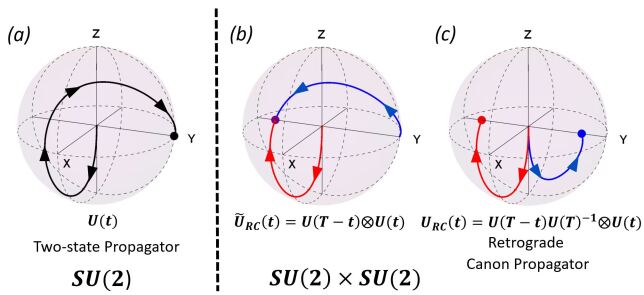
Figure 2: Geometrical description of the quantum retrograde canon - (a) The time evolution of $U:[0,T]\rightarrow SU(2)$, a two-state propagator satisfying $U(T)=R_{\hat{y}}(\pi)$, which is mapped by $\eta$ to the point $(0,1,0)$ - like any propagator, it starts at the identity $I_{2}\in SU(2)$ - which is mapped by $\eta$ to the origin $(0,0,0)$. (b) presents $\tilde{U}^{RC}:[0,T/2]\rightarrow SU(2)\times SU(2)$, with two curves: $\eta(U(t))$, the curve of original propagator (in red), and $\eta(U(T-t))$, a curve which goes backwards along same path (in blue). The two curves meet at time $\tau=T/2$. (c) presents $U^{RC}$, the retrograde canon propagator - the multiplication of $\tilde{U}^{RC}$ by $U(T)^{-}{}^{1}\otimes I_{2}$ transposes the blue curve’s starting point to the origin.

Hence, for the case where $U(T)(1,0)^{\intercal}=(0,1)^{\intercal}$, $\eta(U(t))$ is a curve in the unit 3-ball that goes from the origin $(0,0,0)$ to the boundary point $(0,1,0)$. The curve $\eta(U(T-t))$ goes backwards along the same path. CPT will occur at the inevitable moment when the two curves meet, i.e., at $\tau=T/2$, and possibly at other moments if $\eta(U(t))$ is self-intersecting.

In our first example we examine two-state Hamiltonians of the form:

$$H(t)=-\frac{1}{2}\begin{cases}p\cdot\sigma_{x}&0\text{$\leq$}t<\pi\\ q\cdot\sigma_{z}&\pi\text{$\leq$}t\text{$\leq$}2\pi\end{cases}$$ (21)

where $p,q$ are odd integers. An Hamiltonian of the above form facilitates a $p\pi$-rotation around the the $\hat{x}$-axis, followed by a $q\pi$-rotation around the $\hat{z}$-axis. Such sequences are equivalent to a $\pm\pi$-rotation around the $\hat{y}$-axis. Hence, these Hamiltonians facilitate CPT and satisfy the left hand side of 19 with $|\downarrow\rangle=\pm(0,1)^{\intercal}$ for time $T\equiv 2\pi$. We shall translate $H(t)$ to a four-level system, using the the retrograde canon and the following conjugating matrix $W$

$$W\equiv\frac{1}{\sqrt{2}}\begin{pmatrix}1&\enspace sin(\theta)&0&\enspace cos(\theta)\\ 0&\enspace cos(\theta)&1&-sin(\theta)\\ 0&\enspace cos(\theta)&-1&-sin(\theta)\\ 1&-sin(\theta)&0&-cos(\theta)\end{pmatrix}$$ (22)

where $\theta=-\tan^{-1}(\frac{p}{q})$ . The result, $\mathcal{H^{CRC}}$, is a constant coupling four-state Hamiltonian which facilitates CPT from $\Psi_{1}$ to $\Psi_{3}$ at time $\tau=T/2=\pi$, where

$$\mathcal{H^{CRC}}=n(p,q)\cdot\begin{pmatrix}0&C(p,q)&0&0\\ \ldots&0&B(p,q)&0\\ \ldots&\ldots&0&A(p,q)\\ \ldots&\ldots&\ldots&0\end{pmatrix}$$ (23)

where $n(p,q)=1/\sqrt{p^{2}+q^{2}}$ and $A(p,q),B(p,q),C(p,q)$ are time-constant integers, depending on $p$ and $q$, which satisfy the Pythagorean relation $A^{2}(p,q)+B^{2}(p,q)=C^{2}(p,q)$. The fact that such Hamiltonians perform CPT was derived and utilized in previous works (Suchowski et al., 2011) (Svetitsky et al., 2014). Figure 3 presents the dynamics of the original two-state system and the resulting retrograde canon system.

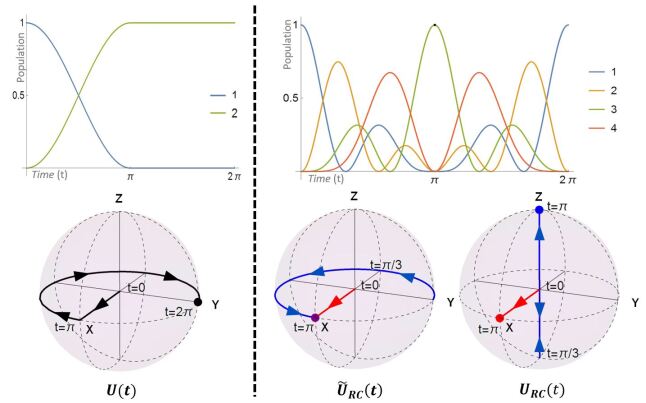
Figure 3: Pythagorean coupling CPT solutions reproduced by applying the retrograde canon to a sequence of $\pi$-rotations. The dynamics for $p=1\enspace,q=3$ in eq. 21, which corresponds to $(A,B,C)=(3,4,5)$ in eq. 23, are presented above. States’ populations vs. interaction time appear in the upper row while the propagator’s path, visualized using $\eta$ (see eq. 20), are in the lower row. The original two-state system, on the left, first makes a $\pi$-rotation around $\hat{x}$-axis - already reaching CPT - and then makes a $3\pi$-rotation around $\hat{z}$-axis - which doesn’t effect the states’ population. The retrograde canon operator undergoes both rotations simultaneously on two independent qubits, reaching CPT when both are complete.

For the second example, we take a two-state time-dependent Hamiltonian that performs CPT through adiabatic following (Vitanov et al., 2001) by means of a Landau-Zener scheme (Landau, 1932)(Rosen and Zener, 1932). We define $H(t)\equiv\vec{h}(t)\cdot\vec{J}^{(2)}$ with

$$\vec{h}(t)=(\Omega_{0},0,B(1-\frac{2t}{\tilde{T}}))$$ (24)

satisfying $B\gg\Omega_{0}^{2}$ and $\Omega_{0}^{2}\gg B/\tilde{T}$ . We define the retrograde Hamiltonian with $T=\tilde{T}$ as the moment of two-state CPT. For $t\approx T$, $U(t)(1,0)^{\intercal}\approx e^{i\alpha(t)}(0,1)^{\intercal}$, with $\alpha(t)$ changing rapidly. Applying the method requires using $\alpha(T)$ in the definition of $W$. Alternatively, we can rotate $H(t)$ around the $\hat{z}$-axis with $H(t)\rightarrow R_{\hat{z}}(-\alpha(T))H(t)R_{\hat{z}}(\alpha(T)$), and use $W$ defined in eq. 22, to get the following time-dependent Hamiltonian:

$$\mathcal{H}_{CRC}(t)=\\ \begin{pmatrix}0&h_{z}(t)sin(\theta)&isin(\alpha)&h_{z}(t)cos(\theta)\\ \ldots&0&-cos(\alpha)sin(\theta)&0\\ \ldots&\ldots&0&cos(\alpha)cos(\theta)\\ \ldots&\ldots&\ldots&0\end{pmatrix}$$ (25)

Figure 4 presents the resulting dynamics. It can be observed in the plot of the original propagator’s dynamics (bottom left), that for $t\ll T/2$ the two-state propagator is approximately a rotation by some angle around $\hat{z}$-axis, while for $t\gg T/2$ it is approximately a rotation by an angle $\pi$ around some axis in the $\hat{x}$-$\hat{y}$ plain (see eq. 20). While this explains the robustness of the two-state dynamics starting at $(1,0)^{T}$, it also explains the transient nature of the CPT in the retrograde canon system: Using eqs. 2,5 and 14 we see that if $t$ is sufficiently far from $T/2$, then $U^{RC}(t)w_{1}\approx F(R_{\hat{z}}(\beta)R_{\hat{y}}(\pi)R_{cos(\gamma)\hat{x}+sin(\gamma)\hat{y}}(\pi))=F(R_{\hat{z}}(\delta))$ with $\beta,\delta\in[0,4\pi)$ $\gamma\in[0,2\pi)$. The low occupancy of the third state for such $t$ is then explained by $0=\langle F(R_{\hat{z}}(\delta)),F(R_{\hat{y}}(\pi))\rangle$ $\forall\delta\in[0,4\pi)$ - where $\text{\textlangle}\cdot,\cdot\text{\textrangle}$ is the standard inner product.

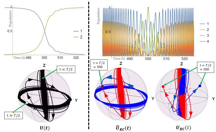
Figure 4: Dynamics of a time-dependent four-level Hamiltonian produced by applying the retrograde canon method to an adiabatic two-state scheme (for $\Omega_{0}=1$, $B=100$$,\tilde{T}=1000$, in eq. (24) and $\theta=\pi/3,$ $\alpha=1.2$ in eq. (25)).

VI optimal and operator control

Next, we indicate ways in which the retrograde canon can be used for optimal control and operator control problems. We begin with optimal control. It is typical for such problems to contain optimization criteria or constraints relating to some norm defined through the parameters of the Hamiltonian (D’Alessandro, 2008). We therefore note that a simple relation between natural norms of the four-state $\mathcal{H}^{CRC}$ and the two-state $H$, holds under the suggested translation method, namely

$$\frac{1}{\sqrt{2}}\|\mathcal{H}^{CRC}(t)\|_{F}=\sqrt{\text{$\|$}\vec{h}(t)\|_{2}^{2}+\|\vec{h}(2\tau-t)\|_{2}^{2}}$$ (26)

where $\vec{h}(t)$ is defines the two-state Hamiltonian through $H(t)=\vec{h}(t)\cdot\vec{J}^{(2)}$, $\|\vec{h}\|_{2}$ is the Euclidean norm and $\text{\textbardbl}\mathcal{H}\text{\textbardbl}_{F}$ is the Frobenius norm defined by $\|\mathcal{H}\|_{F}\equiv\sqrt{\sum|\mathcal{H}{}_{ij}|^{2}}$ . It follows from eq. 26 that

$$\frac{1}{2}\intop_{0}^{\tau}\|\mathcal{H}_{CRC}(t)\|_{F}^{2}\,dt=\intop_{0}^{2\tau}\|\vec{h}(t)\|_{2}^{2}\,dt$$ (27)

Relations such as eqs. 26 and 27 provide a basis for identifying certain multi-state optimal control problems with two-state optimal control problems.

Up to now we have only discussed the retrograde canon in the context of the CPT state-control problem, yet the retrograde canon method may also shed light on operator control problems. Indeed, knowing that $\mathcal{U}^{CRC}$ performs CPT at time $\tau$ holds only partial information on $\mathcal{U}^{CRC}(\tau)$. However, further information regarding $\mathcal{U}^{CRC}(\tau)$ can be related to information on $U(\tau)$ – i.e., the point where the curve of $U(t)$ and $U(T-t)$ meet. Consider, for example, four-state propagator operators of the following form $R=\text{|eg\text{\textrangle}\textlangle}ee|\pm\text{|ee\text{\textrangle}\textlangle}eg|\pm\text{|ge\text{\textrangle}\textlangle}ge|\pm\text{|gg\textrangle\textlangle}gg|$ where $|g\text{\textrangle}$,|e⟩ form a basis of a two-state system and |gg⟩$\equiv\text{|g\textrangle$\otimes$|g\textrangle}$. Operator such as $R$ are universal operators for quantum computation, since they maximally entangle separable states ($R\{\text{|(e+g)$\otimes$e\text{\textrangle}}\}=\text{|ee\text{\textrangle$\pm$}|gg\textrangle}$) and thus satisfy a criterion of being a universal gate (Brylinski and Brylinski, 2002). If we identify $(\Psi_{1},\Psi_{2},\Psi_{3},\Psi_{4})$ with $(\uparrow\uparrow,\uparrow\downarrow,\downarrow\uparrow,\downarrow\downarrow)$, and use the following conjugating matrix

$$W\equiv\frac{1}{\sqrt{2}}\begin{pmatrix}1&0&\enspace i\,sin(\theta)&\enspace i\,cos(\theta)\\ 0&-1&\enspace i\,cos(\theta)&-i\,sin(\theta)\\ 0&1&\enspace i\,cos(\theta)&-i\,sin(\theta)\\ 1&0&-i\,sin(\theta)&-i\,cos(\theta)\end{pmatrix}$$ (28)

then, for $\theta=0$, the condition for getting $\mathcal{U}^{CRC}(\tau)=R$ is that $\eta(U(\tau))$ is either $(0,\pm 1/\sqrt{2},0)$ or $(\pm 1/\sqrt{2},0,\pm 1/\sqrt{2})$. Changing $\theta$ relates the above points to other operators – for example, for $\theta=\pi/4$, the meeting points $(\pm 1/\sqrt{2},0,\pm 1/\sqrt{2})$ correspond to a “double-rail” operator, making the transitions $e_{1}\leftrightarrow e_{2}$ and e${}_{3}\leftrightarrow e_{4}$.

VII generalizations

Last, we present the general version of the method, which allows translating two-level schemes to a wide family of $SU(2)\text{\texttimes}SU(2)$ controlled $n^{2}$-level systems. The generalization is based on relinquishing three assumptions made above which concern: (a) the pace of movement along the dynamical path traced by the original one-qubit Hamiltonian; (b) the dimension of representation of the original Hamiltonian; and (c) the final state of the original system. For a discussion of these assumptions and a proof of following general translation claim see Appendix B.

To carry out the generalization we revise our definitions. We begin by taking a higher order representation of the original Hamiltonian: Given a two-state Hamiltonian, $H(t)$, we define $H^{(n)}(t)$ to be its image in an $n$-dimensional representation. That is,

$$H_{n}(t)\equiv\pi_{n}(H(t))$$ (29)

where $\pi_{n}$ is a $n$-dimensional irreducible representation of $su(2)$, fixed by satisfying $\pi_{n}(J_{i}^{(2)}$)$=J_{i}^{(n)}$ for $i=1,2,3$ where $\vec{J}^{(n)}\equiv(J_{1}^{(n)},J_{2}^{(n)},J_{3}^{(n)})$ satisfies the commutation relation $[J_{i}^{(n)},J_{j}^{(n)}]=i\varepsilon_{ijk}J_{k}^{(n)}$ with a real $J_{1}^{(n)}$ and a diagonal $J_{3}^{(n)}$. Next, we define a $n$-dimensional retrograde Hamiltonian that goes back along the original trajectory in a non-constant pace. That is, we define

$$H_{n}^{R}(t)\equiv-\dot{r}(t)H^{(n)}(T-r(t))$$ (30)

where $0\leq r(t)\leq T$ is a general differentiable function of time. It can be verified by differentiation that $U_{n}^{R}(t)=U_{n}(T-r(t))U_{n}(T)^{-1}$ is the propagator generated by $H_{n}^{R}$, where $U_{n}$ is the $n$-dimensional propagator generated by $H_{n}$. We continue be defining the $n^{2}$-state retrograde canon Hamiltonian, $H_{n}^{RC}$ by

$$H_{n}^{RC}(t)\equiv H_{n}^{R}(t)\text{$\otimes$$I_{2}+I_{2}\otimes H_{n}(t)$}$$ (31)

Clearly $U_{n}^{RC}$, the propagator generated by $H_{n}^{RC}$, satisfies $U_{n}^{RC}(t)=U_{n}^{R}(t)\otimes U_{n}(t)$.

We will also to generalize the definition of $W$, the conjugating matrix defined above in section III: Given $n\in\mathbb{N}$ ,$k\in\{1,\ldots,n-1$}, and a unit vector $\hat{r}\in\mathbb{R}^{3}\enspace(|\hat{r}|=1)$, we shall designate as a $n^{2}$-conjugating matrix of $k$ and $\hat{r}$ any $n^{2}$-dimensional unitary matrix $W(k,\hat{r})=(w_{1},w_{2},...,w_{n^{2}})$ satisfying

$$w_{1}\propto F_{n}(R_{\hat{r}}^{(n)}(\omega_{k})\cdot R_{\hat{y}}^{(n)}(\pi));\enspace w_{2}\propto F_{n}(R_{\hat{y}}^{(n)}(\pi))$$ (32)

where $\omega_{k}\equiv\frac{2k\pi}{n}$, $\hat{R}_{r}^{(n)}(\phi)\equiv e^{i\phi\hat{r}\cdot\vec{J}^{(n)}}$ and $F_{n}$ is the $n$-dimensional analog of the flattening function $F$ encountered in eq. 14, i.e., it takes a $n$-by-$n$ matrix and returns a $n^{2}$column vector defined by $F(m)_{(n-1)i+j}\equiv m_{ij}$.

Now, we can define the $n^{2}$-state conjugated retrograde canon Hamiltonian:

$$\mathcal{H}_{n}^{CRC}(t)\equiv W_{n}(k,\hat{r})^{\intercal}H_{n}^{RC}(t)W_{n}{(k,\hat{r})}.$$ (33)

Its corresponding propagator, $\mathcal{U}_{n}^{CRC}$, of course satisfies $\mathcal{U}_{n}^{CRC}=W_{n}(k,\hat{r})^{\intercal}U_{n}^{RC}W_{n}{(k,\hat{r})}$

Finally, we formulate the general translation claim: Let there be $k,\>\hat{r}$, a $n^{2}$-state conjugating matrix $W_{n}(k,\hat{r})$, a differentiable pace function $r:[0,T]\rightarrow\mathbb{{R}}$ and a two-state system Hamiltonian $H:[0,T]\rightarrow su(2),$ whose propagator is $U(t)$. Then, $\forall\tau\in(0,T)$ for which $U(T-r(\tau))=U(\tau)$ the following holds:

$$U(T)=\pm R_{\hat{r}}(\omega_{k})\Leftrightarrow 1=|\text{\textlangle}e_{2},\mathcal{U}_{n}^{CRC}(\tau)e_{1}\text{\textrangle}|$$ (34)

where $e_{i}\in\mathbb{C}^{n^{2}}i=1,2$ are standard basis vectors. In particular, for any time $\tau_{x}$ for which $T-r(\tau)=\tau$, $\mathcal{H}_{n}^{CRC}$ facilitates the transition $e_{1}\rightarrow e_{2}$ at time $\tau\in(0,T)$ if and only if $U(T)=R_{\hat{r}}(\omega_{k})$. Note that for even $n$ we could take $k=n/2\enspace\text{$\in$}\mathbb{N}$ and $\hat{r}=\hat{y}$ to get $U(T)=R_{\hat{y}}^{(n)}(\pi)$ and $w_{1}\propto F_{n}(R_{\hat{y}}^{(n)}(\pi))$ for eqs. 34 and 32 respectively – such a choice would be a straight forward generalization of the four-state translation method, one which converts two-state CPT schemes to $n^{2}$-state CPT schemes.

VIII conclusion

In conclusion, we introduced a novel method for translation between multi-state control problems and two-state systems. The method provides a new framework for importing the knowledge, tools and intuition related to two-state systems, into multi-state research. In particular, the method offers an exact reduction into two-state systems of multi-state CPT problems that cannot be reduced by available methods. The idea of the retrograde canon in control theory can be further explored in future research: e.g., in the application of the retrograde canon to other groups that have appropriate properties, such as $Sp(n)\rightarrow Sp(n)\times Sp(n)$ instead of $SU(2)\rightarrow SU(2)\times SU(2)$ or in using $k$ two-states CPT schemes together to generate a CPT scheme in a $\underbrace{SU(2)\times SU(2)\times...\times SU(2)}_{2k}$ controlled system. We hope that the analytical reduction of multi-state control problems to two-state systems offered by the quantum retrograde canon may be helpful for a deeper understanding of multi-state dynamics, and in simplifying the analysis in certain cases of particular interest.

Appendix A The general form of the conjugating matrix

We shall now present and explain the general form of the four-state conjugating matrix $W$, and general form of $\mathcal{H}^{CRC}(t)$ derived from it. Remember that $w_{2},w_{4}\in\mathbb{C}^{4}$ can be chosen to be any two vectors that complete $e^{i\phi_{1}}w_{1},e^{i\phi_{3}}w_{3}$ to an orthonormal basis of $\mathbb{C}^{4}$. This gives the choice of $W$ six degrees of freedom: the angle $\alpha$ in the definition of $|\downarrow\rangle$, the four phases of the four vectors, and the orientation of $w_{3}$ and $w_{4}$ in the subspace orthogonal to $span\{w_{1},w_{2}\}$. Since one degree of freedom can be regarded as a global phase which changes nothing in the shape of $H(t)$, we effectively have only five degrees of freedom. To slightly simplify the presentation we set $\alpha=0$ in what follows and place $w_{3}$ in the second column of $W$. We can organize these degrees of freedom by first defining a basic alternative $\tilde{W}=\{\tilde{w_{1}},\tilde{w_{3}},\tilde{w_{2}},\tilde{w_{4}}\}$ with

$$\tilde{w_{1}}\equiv\frac{1}{\sqrt{2}}F_{2}(I_{2})=\frac{1}{\sqrt{2}}(1,0,0,1)^{\intercal}$$

$$\tilde{w_{3}}\equiv-\frac{1}{\sqrt{2}}F_{2}(R_{\hat{y}}(\pi))=\frac{1}{\sqrt{2}}(0,1,-1,0)^{\intercal}$$

$$\tilde{w_{2}}\equiv-iF_{2}(R_{\hat{x}}(\pi))=\frac{1}{\sqrt{2}}(0,1,1,0)^{\intercal}$$

$$\tilde{w_{4}}\equiv-iF_{2}(R_{\hat{z}}(\pi))=\frac{1}{\sqrt{2}}(1,0,0,-1)^{\intercal}$$

Note that $\tilde{W}$ is just a permutation of the columns of $W$ defined in (9). Next, we define the general form of the conjugating matrix $W\equiv\{w_{1},w_{3},w_{2},w_{4}\}$ , using four variables, $\phi_{2},\phi_{3},\phi_{4},\theta\in[0,2\pi)$ to be

$$w_{1}\equiv\tilde{w_{1}}$$

$$w_{3}\equiv e^{i\phi_{3}}\tilde{w_{3}}$$

$$w_{2}\equiv e^{i\phi_{3}}(cos(\theta)\tilde{w}_{3}+sin(\theta)\tilde{w}_{4})$$

$$w_{4}\equiv e^{i\phi_{4}}(cos(\theta)\tilde{w}_{4}-sin(\theta)\tilde{w}_{3})$$

to finally get the general form of $W$

$$W\equiv\frac{1}{\sqrt{2}}\begin{pmatrix}1&0&\enspace e^{i\phi_{3}}sin(\theta)&\enspace e^{i\phi_{4}}cos(\theta)\\ 0&e^{i\phi_{2}}&\enspace e^{i\phi_{3}}cos(\theta)&-e^{i\phi_{4}}sin(\theta)\\ 0&e^{-i\phi_{2}}&\enspace e^{i\phi_{3}}cos(\theta)&-e^{i\phi_{4}}sin(\theta)\\ 1&0&-e^{i\phi_{3}}sin(\theta)&-e^{i\phi_{4}}cos(\theta)\end{pmatrix}$$ (35)

We proceed to present the form of $\mathcal{H}^{CRC}$, the form of the Hamiltonian resulting from a general two state system Hamiltonian and a choice of $W$. The general form of $\mathcal{H}^{CRC}$ shows which four state Hamiltonians can be translated by the retrograde canon method to a two-level system. We parameterize the two-state Hamiltonian by writing $H(t)=\frac{1}{2}\vec{h}(t)\cdot\vec{\sigma}$ where $\vec{h}(t)\equiv(h_{x}(t),h_{y}(t),h_{z}(t))\in\mathbb{R}^{3}$. Then, in order to simplify the form of $\mathcal{H}^{CRC}(t)$ we introduce the vectors $\vec{A^{\pm}}(t)\equiv(a^{\pm}(t),b^{\pm}(t),c^{\pm}(t))\equiv\frac{\vec{h}(t)\text{\textpm}\vec{h}(T-t)}{2}$ and $\vec{A}_{\theta}^{\pm}\equiv(a_{\theta}^{\pm}(t),b^{\pm}(t),c_{\theta}^{\pm}(t))$ which are defined from $\vec{A^{\pm}}(t)$ through a rotation of $\theta$ around $\hat{y}$-axis, i.e., $a_{\theta}^{\pm}(t)=cos(\theta)a^{\pm}(t)+sin(\theta)c^{\pm}(t)$ and $c_{\theta}^{\pm}(t)=cos(\theta)c^{\pm}(t)-sin(\theta)a^{\pm}(t)$. we finally get the general matrix form of $\mathcal{H}^{CRC}(t)$, presented in terms of the parameters of $H(t)$ and the degrees of freedom inherited from $W$ :

$$\mathcal{H}^{CRC}(t)=\\ \begin{pmatrix}0&-ie^{i\phi_{2}}b^{+}(t)&e^{i\phi_{3}}a_{\theta}^{-}(t)&e^{i\phi_{4}}c_{\theta}^{-}(t)\\ \ldots&0&-e^{i(\phi_{3}-\phi_{2})}c_{\theta}^{+}(t)&e^{i(\phi_{4}-\phi_{2})}a_{\theta}^{+}(t)\\ \ldots&\ldots&0&ie^{i(\phi_{4}-\phi_{3})}b^{-}(t)\\ \ldots&\ldots&\ldots&0\end{pmatrix}$$ (36)

The under-diagonal entries in eq. 36 follow from Hermiticity. A permutation of the conjugating matrix columns (see eq. 35) would shuffle the places of the “$a,b,c"$ letters and $"+/-$” signs in eq. 36.

We note that with an appropriate choice of $\phi_{2},\phi_{3},\phi_{4}$ all six above-diagonal entries of $\mathcal{H}^{CRC}(t)$ in eq. 36 can be set imaginary, yet no more than four can be real. There are three possible ways to get four real above-diagonal entries - in each, either the couple $(a_{\theta},A_{\theta})$ or $(b_{\theta},B_{\theta})$ or $(c_{\theta},C_{\theta})$ will have imaginary coefficients. Figure 2 presents an example of such couplings. Suppose we wonder whether $\mathcal{H}(t)$, a Hamiltonian of the form in eq. 36 performs CPT at time $\tau$. Such questions can be reduced to questions regarding a two-state Hamiltonian $H(t)$ by applying the method backwards, i.e., by inverting eq. 18 - while taking suitable phase parameters $\phi_{i}\enspace(i=2,3,4)$ and choosing $\theta\in[0,2\pi)$ at will - followed by applying eq. 6. The resulting two-state Hamiltonian $H(t)$ would facilitate CPT from $|\uparrow\rangle$ to $|\downarrow\rangle$ at time $2\tau$ if and only if the four-state Hamiltonian $\mathcal{H}(t)$ would evolve the state $e_{1}$ to $\pm e_{2}$ at time $\tau$.

Appendix B The general translation claim - discussion and proof

The general version of the retrograde canon method allows translating two-level schemes to a wide family of $SU(2)\times SU(2)$ controlled $n^{2}$-level systems. The definitions of the general method and its corresponding general translation claim appear in eqs. (31)-(34) in the main text. The first part of this appendix is concerned with explaining the rational behind the generalization, while the second part contains a proof of the general translation claim.

B.1 A discussion of the generalizations

We recall that the method’s general version is based on relinquishing three assumptions that underlie the fundamental version - assumptions which concern: (a) the pace of movement along the path of the original propagator; (b) the dimension of representation of the original Hamiltonian; and (c) the final state of the original system. Let us explain the rational of dropping these three assumptions.

We begin with (a), the pace of movement along the path of the original propagator. The definition of $H^{RC}$, given in eq. (30), is such that $U(t)$ and $U^{R}(t)$ move at the same constant pace (albeit in opposite directions). This, however, is not a necessary condition for the method to work. The propagator, $U^{R}$ can move at practically any pace, $\dot{r}(t)$, so long as there’s a moment $\tau$ for which $U(T-r(\tau))=U(\tau)$ – which always happens for a time $\tau_{r}\in[0,T]$ such that $T-r(\tau_{r})=\tau_{r}$. Thus, by loosening the pace assumption allows creating a wide family of significantly different multi-state Hamiltonians, even if the pace is constant (i.e. $r(t)=at$ for some $a>0$). Changing the pace can be used to move $U(\tau_{r})$ - the meeting point of $U(t)$ and $U(T-t)$ - which defines the operator $\mathcal{U}^{CRC}(\tau_{r})$, to any point along the path of $U(t)$.

Next, consider assumption (b), concerning the dimension of representation of the original Hamiltonian: We shall see in the proof of the general translation claim below that in the definition of the retrograde canon Hamiltonian we need not restrict ourselves to using the fundamental representation of the original Hamiltonian. Correspondingly, the output system does not have to be a four-level system. Rather, it can be a $n^{2}$-state system for every $n\in\mathbb{N}$. The change of dimension of the retrograde canon Hamiltonian has to be accompanied by a non-trivial revision of the definition of the conjugating matrix $W$. One natural way of revising $W$ - which is appropriate only for even $n$ - is defining the $n^{2}$-state conjugating matrix as any $n^{2}$-dimensional unitary matrix $W_{n}=\{w_{1},w_{2},...,w_{n^{2}}\}$ such that

$$w_{1}\propto F_{n}(I_{n});\enspace w_{2}\propto F_{n}(R_{\hat{y}}^{(n)}(\pi))$$

where $F_{n}$ is the flattening function presented in (32). Note, that while $I_{n}$ has $1$s on the diagonal, and $0$s everywhere else, the matrix $R_{\hat{y}}^{(n)}(\pi)$ has $1$s and $(-1)$s alternately on the anti-diagonal, and $0$s everywhere else. Therefore, since for even $n$ the anti-diagonal and the diagonal of a $n$-dimensional matrix have no common entry, $w_{1}$ and $w_{2}$ will indeed by orthogonal for every even $n$. On the other hand, for odd $n$, the anti-diagonal and the diagonal do have a common entry, and therefore $F_{n}(I_{n})$ and $F_{n}(R_{\hat{y}}^{(n)}(\pi))$ will not be orthogonal and cannot be columns of the same unitary matrix.

The generalization of the third assumption (c), regarding the final state of the original system $U(T)$, is designed to solve the above mentioned problem of odd $n$ representations. In the process, it opens up the method to a wider range of conjugating matrices and two-state schemes, thus enabling the production of a wider variety of $n^{2}$-state CPT schemes – useful also for even $n>2$. The generalization with regards the final state of the original system, $U(T)$, comes from the insight that the method and the translation claim essentially rely on just three basic conditions (assuming for the moment that $\alpha=0$). To present these conditions we mark the first two columns of the required $n^{2}$-state conjugating matrix as $w_{1}\equiv F_{n}(m_{1})$ and $w_{2}\equiv F_{n}(m_{2})$.

The first condition is that

$$U_{n}(T)^{-1}m_{1}=m_{2}$$ (37)

The second condition is that

$$m_{2}=R_{\hat{y}}^{(n)}(\pi)$$ (38)

The third condition is that

$$F_{n}(m_{1})\perp F_{n}(m_{2})$$ (39)

The last condition simply ensures that $w_{1}$ and $w_{2}$ are orthogonal and can therefore be two columns in the same unitary matrix. The role of the first two conditions shall be clarified in the proof below. If these conditions are satisfied we can define as the $n^{2}$-state conjugating matrix any unitary matrix whose first two columns are $F_{n}(m_{1})$ and $F_{n}(m_{2})$, and formulate a general translation claim for two-state systems whose final states satisfy (37), i.e. $U_{n}(T)=m_{2}m_{1}^{-1}$.

Interestingly, assuming eqs. (37) and (38), all that is needed to satisfy eq. (39) is that $U(T)$, the original propagator at time $T$, should satisfy

$$\chi_{n}(U(T))=0$$ (40)

Where $\chi_{n}:SU(2)\rightarrow\mathbb{C}$ is the character of the $n$-dimensional irreducible representation of $SU(2)$ ,i.e., the function which for every element of $SU(2)$ returns the trace of its image in the $n$-dimensional irreducible representation. Hence, (40) is equivalent to

$$trace(U_{n}(T))=0$$ (41)

We shall now prove that indeed, if eqs. (37) and (38) are satisfied then eq. (41) follows from (39). We mark $Y_{n}=R_{\hat{y}}^{(n)}(\pi)$. Now, from (37) and (38) we get $m_{2}\equiv\pm Y_{n}$ and $m_{1}\equiv U_{n}(T)Y_{n}$. Therefore,

$$\langle F_{n}(m_{1}),F_{n}(m_{2})\rangle=\langle F_{n}(U_{n}(T)Y_{n}),F_{n}(Y_{n})\rangle$$ (42)

Note that for every $A,B\in M_{n}(C)$ the following identity holds

$$\langle F_{n}(A),F_{n}(B)\rangle=\langle F_{n}(AY_{n}),F_{n}(BY_{n})\rangle$$ (43)

Eq. (43) can be understood as following from the form of $Y_{n},$ whose only non-zero entries are $1$s and $(-1)$s on the anti-diagonal. Therefore, multiplication by $Y_{n}$ from the right simply permutes the columns of the multiplied matrix while providing factors of $\pm 1$. Hence, applying $Y_{n}$ to the matrices on both sides of the inner product only changes the order of summation and not the result. Using (43), and noting the fact that $Y_{n}Y_{n}=-I_{n}$, we see that under assumptions (37) and (38), eq. (39) is indeed equivalent to (40), since

$$0=\text{\textlangle}F_{n}(m_{1}),F_{n}(m_{2})\text{\textrangle}=\text{\textlangle}F_{n}(U_{n}(T)Y_{n}),F_{n}(Y_{n})\text{\textrangle}\\ =\text{\textlangle}F_{n}(U_{n}(T)),F_{n}(I_{n})\text{\textrangle}=trace(U_{n}(T))=\chi_{n}(U(T))$$ (44)

We shall now present and prove a criterion for a matrix $U(T)\in SU(2)$ to satisfy eq. (40): For every unit vector $\hat{r}\in\mathbb{R}^{3}$ the following equivalence holds

$$\chi_{n}(R_{\hat{r}}(\omega))=0\Leftrightarrow\omega=2k\pi/n$$ (45)

$k\in Z,k\neq 0$. To prove (45) we note that for every unit vector $\hat{r}\in\mathbb{R}^{3}$ there exists, $\tilde{\pi}_{n}:SU(2)\rightarrow M_{n}[\mathbb{{C}}$], an irreducible $n$-dimensional representation of $SU(2)$, for which $\tilde{R}_{\hat{r}}^{(n)}(\omega)\equiv\tilde{\pi}_{n}(R_{\hat{r}}(\omega))$ is diagonal. In such a representation we have

$$\tilde{R}_{\hat{r}}^{(n)}(\omega)=\begin{pmatrix}e^{ij\omega}\\ &e^{i(j-1)\omega}\\ &&\ddots\\ &&&e^{-ij\omega}\end{pmatrix}$$ (46)

where $j=(n-1)/2$. Therefore

$$trace(\tilde{R}_{\hat{r}}^{(n)}(\omega))=\sum_{m=1-n}^{n-1}e^{im\omega/2}=\begin{cases}\frac{sin(n\omega/2)}{sin(\omega/2)}&\omega\neq 0\\ n&\omega=0\end{cases}$$ (47)

from which (45) follows. To summarize the discussion of assumption (c), regarding the final state of the original system, we see that conditions (37)-(39) entail that $U_{n}(T)=(R_{\hat{r}}(2k\pi/n))$ for $k\in Z,k\neq 0$, and ensure that the definition of the $n^{2}$-state conjugating matrix given in eq. (32) can be satisfied, since the first two columns are orthogonal. The fact that under definition (32), the general translation claim, given in eq. (34), follows, is what we shall now prove.

B.2 A proof of the general translation claim

We need a some more preparation before presenting the proof. We shall use the fact that a high order representation of a propagator is a propagator of the high order Hamiltonian, i.e., that for all $t\in[0,T]$ we have

$$\Pi_{n}(U(t))=U_{n}(t)$$ (48)

where $\Pi_{n}:SU(2)\rightarrow M_{n}(\mathbb{C})$ is the lie group representation of $SU(2)$ which for every $R_{\hat{r}}(\phi)\in SU(2)$ satisfies

$$\Pi_{n}(R_{\hat{r}}(\phi))\equiv R_{\hat{r}}^{(n)}(\phi)$$ (49)

Eq. (48) follows directly from the fact that $H_{n}(t)\equiv\pi_{n}(H(t))$ where $\pi_{n}:su(2)\rightarrow M_{n}[\mathbb{C}]$, is the $n$-dimensional lie algebra linear representation of $su(2)$, fixed by $\pi_{n}(J_{i}^{(2)})=J_{i}^{(n)}$ for $i=1,2,3$. This can be proved by writing $U_{n}(t)=R_{\hat{n(t)}}^{(n)}(\phi_{n}(t))$ where $\phi_{n}:[0,T]\rightarrow\mathbb{R}$ and $\hat{r}_{n}:[0,T]\rightarrow\mathbb{S}^{2}\subset\mathbb{R}^{3}$, and showing that for every $n\geq 2$, $\phi_{n}=\phi_{2}$ and $\hat{r}_{n}=\hat{r}_{2}$. Indeed, from (48) and (49) it follows that the left side of eq. (34) means that $U_{n}(T)$ satisfies

$$U_{n}(T)=R_{\hat{r}}^{(n)}(\omega_{k})$$ (50)

Another important fact for the proof is that the analog of eqs. (14) and (15) also holds for higher dimensional irreducible representations of $SU(2)$ - i.e., that for every $u_{n}\in\Pi_{n}(SU(2))$ the following equation holds

$$Y_{n}=u_{n}Y_{n}u_{n}{}^{\intercal}$$ (51)

We shall prove (51) using the defining property of group representations, which is that the multiplication of images of group elements under the representation equals the image of the multiplication of the group elements. Hence, together with eqs. (15), (49), and the fact that there exists $u\in SU(2)$ such that $u_{n}=\Pi_{n}(u)$ we get

$$Y_{n}=\text{\leavevmode{P}}_{n}(Y)=\text{\leavevmode{P}}_{n}(uYu^{\intercal})=\\ \text{\leavevmode{P}}_{n}(u)\text{\leavevmode{P}}_{n}(Y)\text{\leavevmode{P}}_{n}(u^{\intercal})=u_{n}Y_{n}u_{n}{}^{\intercal}$$ (52)

we have assumed in eq. (52) that $u^{\intercal}\in SU(2)$ and that $\Pi_{n}(u^{\intercal})=(\Pi_{n}(u))^{\intercal}$ – which are facts that can be proved, for instance, using Euler decomposition of $u\in SU(2)$ as $u=R_{\hat{y}}(\alpha)R_{\hat{z}}(\beta)R_{\hat{y}}(\gamma)$.

After these preliminaries we can proceed to prove the general translation claim, given in eq. (34). We begin with the $\Rightarrow$ direction of eq. (34). We shall use the assumptions that $U(T-r(\tau))=U(\tau)$ and that $U(T)=\pm R_{\hat{r}}(\omega_{k})$ and conclude that $1=|\langle e_{2},U_{n}^{CRC}(\tau)e_{1}\rangle|$. First, note that$\langle e_{2},U_{n}^{CRC}(\tau)e_{1}\rangle=\langle w_{2},U_{n}^{RC}(\tau)w_{1}\rangle$. From eq. (48) it follows that

$$U_{n}(T-r(\tau))=U_{n}(\tau)$$ (53)

We will proceed to show that

$$w_{2}=\pm U_{n}^{RC}(\tau)w_{1}$$ (54)

from which the conclusion follows. from eqs. (50) and (53) we see that

$$U_{n}^{RC}(\tau)w_{1}=(U_{n}(\tau)R_{\hat{r}}^{(n)}(\omega_{k})^{-1}\otimes U_{n}(\tau))w_{1}$$ (55)

from which, using eqs. (32), the generalization of (14) and (51), we get

$$U_{n}^{RC}(\tau)w_{1}=\\ F_{n}(U_{n}(\tau)R_{\hat{r}}^{(n)}(\omega_{k}){}^{-1}R_{\hat{r}}^{(n)}(\omega_{k})Y_{n}U_{n}(\tau){}^{\intercal})\\ =\pm F_{n}(U_{n}(\tau)Y_{n}U_{n}(\tau)^{\intercal})\\ =\pm F_{n}(Y_{n})=\pm w_{2}$$ (56)

For the $\Leftarrow$ direction of eq. (34) we shall assume that $U(T-r(\tau))=U(\tau)$ and that $1=|\langle e_{2},U_{CRC}^{(n)}(\tau)e_{1}\rangle|$ to conclude that $U(T)=R_{\hat{r}}(\omega_{k})$. From the assumption it follows that

$$e^{i\alpha}e_{2}=U_{n}^{CRC}(\tau)e_{1}$$ (57)

for some $\alpha\in[0,2\pi)$. Or equivalently,

$$e^{i\alpha}w_{2}=U_{n}^{RC}(\tau)w_{1}=(U_{n}^{R}(\tau)\otimes U_{n}(\tau))w_{1}$$ (58)

Hence, marking $\tilde{R}\equiv R_{\hat{r}}^{(n)}(\omega_{k})Y_{n}$ and $V\equiv U_{n}^{R}(\tau)\tilde{R}Y_{n}U_{n}^{-1}(\tau)$ and noting that $Y_{n}^{-1}=\pm Y_{n}$ (where the sign depends on whether $n$ is even) we get that

$$\begin{array}[]{c}e^{i\tilde{\alpha}}Y_{n}=F^{-1}((U_{n}^{R}(\tau)\otimes U_{n}(\tau))F(\tilde{R}))=\\ =U_{n}^{R}(\tau)\tilde{R}U_{n}(\tau)=\pm VU_{n}(\tau)Y_{n}U_{n}^{\intercal}(\tau)=\pm VY_{n}\end{array}$$

where $\tilde{\alpha}\in[0,2\pi).$ we get

$$e^{i\tilde{\alpha}}Y^{(n)}=a^{(n)}Y^{(n)}$$ (59)

Hence $V=\pm e^{i\tilde{\alpha}}I_{n}$. Since $V\in\Pi_{n}(SU(2))\subset SU(n)$ it follows that $1=|V|=|\pm e^{i\tilde{\alpha}}I_{n}|=(\pm 1)^{n}e^{in\tilde{\alpha}}\Rightarrow$ $\tilde{\alpha}=2\pi k/n$ with $k\in\{0,1,\text{\ldots}n-1\}$. hence $V=(\pm 1)^{n}e^{i2\pi k/n}I_{n}$. Yet an irreducible representations of $SU(2)$ may contain only $I_{n}$ and possibly $-I_{n}$. Hence, we finally get $V=\pm I_{n}$ and $U_{n}^{R}(\tau)=U_{n}(\tau)Y_{n}\tilde{R}^{-1}.$ From which it follows that

$$\begin{array}[]{c}U(T)=(U_{n}^{R}(\tau))^{-1}U_{n}(\tau)=\pm\tilde{R}Y_{n}(U_{n}(\tau))^{-1}U_{n}(\tau)=\\ =\pm\tilde{R}Y_{n}=\pm R_{\hat{r}}^{(n)}(\omega_{k})\end{array}$$

References

- Lanyon et al. (2009) B. P. Lanyon, M. Barbieri, M. P. Almeida, T. Jennewein, T. C. Ralph, K. J. Resch, G. J. Pryde, J. L. O’Brien, A. Gilchrist, and A. G. White, Nat. Phys. 5, 134 (2009).
- Cerf et al. (2002) N. J. Cerf, M. Bourennane, A. Karlsson, and N. Gisin, Phys. Rev. Lett. 88, 127902 (2002).
- Nielsen and Chuang (2002) M. A. Nielsen and I. L. Chuang, Quantum Computation and Quantum Information (Cambridge, 2002).
- Sørensen and Mølmer (1999) A. Sørensen and K. Mølmer, Phys. Rev. Lett. 82, 1971 (1999).
- Allen and Eberly (1975) L. Allen and J. H. Eberly, Optical Resonance and Two-Level Atoms (Wiley, 1975).
- Torosov and Vitanov (2008) B. T. Torosov and N. V. Vitanov, Journal of Physics A: Mathematical and Theoretical 41, 155309 (2008).
- Romano and D’Alessandro (2016) R. Romano and D. D’Alessandro, Journal of Physics A: Mathematical and Theoretical 49, 345303 (2016).
- Genov et al. (2011) G. T. Genov, B. T. Torosov, and N. V. Vitanov, Phys. Rev. A 84, 063413 (2011).
- Solá et al. (1999) I. R. Solá, V. S. Malinovsky, and D. J. Tannor, Phys. Rev. A 60, 3081 (1999).
- Paulisch et al. (2014) V. Paulisch, H. Rui, H. K. Ng, and B.-G. Englert, The European Physical Journal Plus 129, 12 (2014).
- Hioe (1987) F. T. Hioe, J. Opt. Soc. Am. B 4, 1327 (1987).
- Bach (1747) J. S. Bach, “Canon no. 1. a 2 cancrizans the musical offering,” (1747).
- Suchowski et al. (2011) H. Suchowski, Y. Silberberg, and D. B. Uskov, Phys. Rev. A 84, 013414 (2011).
- Svetitsky et al. (2014) E. Svetitsky, H. Suchowski, R. Resh, Y. Shalibo, J. M. Martinis, and N. Katz, Nat Commun (2014).
- Vitanov et al. (2001) N. V. Vitanov, T. Halfmann, B. W. Shore, and K. Bergmann, Annu. Rev. Phys. Chem. 52, 763 (02001).
- Landau (1932) L. Landau, in Proc. R. Soc. Lond. Ser. A, Vol. 137 (1932) p. 696.
- Rosen and Zener (1932) N. Rosen and C. Zener, Phys. Rev. 40, 502 (1932).
- D’Alessandro (2008) D. D’Alessandro, Introduction to quantum control and dynamics (Chapman & Hall/CRC, 2008).
- Brylinski and Brylinski (2002) J.-L. Brylinski and R. Brylinski, Mathematics of Quantum Computation 79 (2002).