Multivariable signatures, genus bounds and –solvable cobordisms
Abstract.
We refine prior bounds on how the multivariable signature and the nullity of a link change under link cobordisms. The formula generalizes a series of results about the 4-genus having their origins in the Murasugi-Tristram inequality, and at the same time extends previously known results about concordance invariance of the signature to a bigger set of allowed variables. Finally, we show that the multivariable signature and nullity are also invariant under –solvable cobordism.
1. Introduction
Given , the Levine-Tristram signature and nullity of a link are given by the signature and nullity of , where is any Seifert matrix for [Lev69, Tri69]. For a -colored link, i.e. an oriented link in whose components are partitioned into sublinks , the Levine-Tristram signature and nullity have been generalized to multivariable functions
where denotes the set [CF08]. Apart from their -dimensional definition using C-complexes [Coo82, CF08], a -dimensional interpretation in the smooth setting has been given by Cimasoni-Florens using branched covers and the -signature theorem for elements of of finite order [CF08, Theorem 6.1]. We focus on another interpretation by Viro [Vir09] using directly the complements of surfaces bounding the link in the -ball.
We shall always work in the topological (locally flat) category. Let be a union of properly embedded locally flat surfaces that only intersect each other transversally in double points and whose boundary is a colored link . Since the first homology group of the exterior of such a colored bounding surface is free abelian, any choice of gives rise to a coefficient system and thus to a twisted signature . The twisted signature is independent of the colored bounding surface and defines an invariant of colored links [Vir09, Section 2.3]. Building on [CFT16, Theorem 1.3], we give a proof to the following statement of [Vir09, Section 2.5] in Proposition 3.5. The corresponding result for the nullity is proven in Proposition 3.4.
Proposition 1.1.
Let be a -colored link and let . For any colored bounding surface , the twisted signature coincides with the multivariable signature .
Cimasoni and Florens showed that the signature is invariant under smooth link concordance [CF08, Theorem 7.1] for those that satisfy the following condition: there exists a prime such that for all , the order of is a power of . For the same subset of , they provide lower bounds on the genus and on the number of double points of smooth surfaces in bounded by a colored link [CF08, Theorem 7.2], extending the Murasugi-Tristram inequality [Mur65, Tri69] to the multivariable setting.
Building on the approach used in [NP17] to study concordance invariance of the Levine-Tristram signature, we consider the subset of given by those ’s which are not roots of any polynomial whose evaluation on is invertible. This set includes the elements considered by Cimasoni and Florens [CF08, Section 7]; see Proposition 2.17. A colored cobordism between two -colored links and is a collection of properly embedded locally flat surfaces in which have the following properties: the surfaces only intersect each other transversally in double points, each surface has boundary , and each connected component of has at least one boundary component in and one in . Our first main result gives bounds on the Euler characteristic and on the number of double points in such a cobordism, generalizing Powell’s treatment of a genus bound for the Levine-Tristram signature [Pow17].
Theorem 1.2.
Let be a colored cobordism between two -colored links and . If has double points, then
for all .
Two -colored links and are concordant if there exists a -colored cobordism between and that has no intersection points and consists exclusively of annuli. As an application of Theorem 1.2, we extend two different results of Cimasoni and Florens to the topological setting and to a bigger set of values of the variable . The first result relaxes the conditions under which the signature and nullity are an obstruction to colored concordance [CF08, Theorem ]. See Corollary 3.13 for a proof.
Corollary 1.3.
The multivariable signature and nullity are topological concordance invariants at all
As a second consequence of Theorem 1.2, we obtain a generalization of [CF08, Theorem ]; the latter result being itself an extension of the Murasugi-Tristram inequality [Mur65, Tri69]. In what follows, we denote the first Betti number of a surface by . We refer the reader to Corollary 3.15 for a proof of the next result and to Remark 3.17 for a comparison with a similar result obtained by Viro [Vir09, Section ].
Corollary 1.4.
Let be a colored bounding surface for a -colored link such that have a total number of connected components, intersecting in double points. Then, for all , we have
The last part of this article deals with -solvable cobordisms. This notion was defined by Cha [Cha14] giving a relative version of the notion of Cochran-Orr-Teichner’s -solvability [COT03]. We refer to Section 5 for the precise definition of -solvable cobordant links, however note that abelian link invariants are not expected to distinguish -solvable cobordant links. For instance, if two links are -solvable cobordant, then their first non-zero Alexander polynomials agree up to norms and their Blanchfield pairings are Witt equivalent [Kim15, Theorems and ]. Our final result is the corresponding statement for the multivariable signature and nullity.
Theorem 1.5.
If two -colored links and are -solvable cobordant, then
for all .
Since concordant links are -solvable cobordant for all , Theorem 1.5 can be viewed as a vast refinement of Corollary 1.3.
Remark 1.6.
Note that the notion of -solvable cobordism is related to Whitney tower/grope concordance. See [Cha14] for the definition of these notions. In particular, using [Cha14, Corollary 2.17], Theorem 1.5 implies that the multivariable signature and nullity are invariant under height Whitney tower/grope concordance.
Remark 1.7.
The Alexander nullity of a colored link is the -rank of its Alexander module. Kim [Kim15, Theorem C] showed that the Alexander nullity is invariant under -solvable cobordisms. In Proposition 5.11, we improve this result by proving invariance under -solvable cobordisms. Note also that this statement does not follow from the invariance of the nullity function since [CCZ16, Proposition 2.3].
This paper is organized as follows. Section 2 introduces the necessary background material on twisted homology and signatures. Section 3 introduces the colored signature and nullity and proves Theorem 1.2 together with its applications. Section 4 introduces plumbed -manifolds and proves some results about their signature defects. These form the technical foundation for the proof of Theorem 1.5, which is the subject of Section 5.
Acknowledgments.
We thank Christopher Davis for sharing his insights of –solvability, which helped us immensely in navigating through the technicalities of Section 5. The authors wish to thank Ana Lecuona, David Cimasoni, Vincent Florens, Stefan Friedl, Paul Kirk, Andrew Nicas and Mark Powell for helpful discussions. We are indebted to the referees for their detailed and helpful suggestions. AC thanks UQÀM for its hospitality and was supported by the NCCR SwissMap funded by the Swiss FNS. MN is grateful for his stay at the University of Regensburg funded by the SFB 1085, which started the project. ET was supported by the GK “Curvature, Cycles and Cohomology”, funded by the Deutsche Forschungsgemeinschaft (DFG). MN was supported by a CIRGET postdoctoral fellowship, and by a Britton postdoctoral fellowship from McMaster University.
2. Twisted homology, signatures and concordance roots
In Section 2.1, we set up the conventions on twisted homology. In Section 2.2, we review twisted intersection forms, which leads us to discuss the additivity of the signature in Section 2.3. In Section 2.4, we generalize the concept of Knotennullstellen [NP17].
2.1. Twisted homology
We start by fixing some notation and conventions regarding twisted homology. After that, we review two universal coefficient spectral sequences and apply them to a particular abelian coefficient system.
Let be a connected CW-complex and let be a possibly empty subcomplex. Denote by the universal cover of and set , so that is a left -module. Given a ring with involution, we can consider homomorphisms of rings with involutions, which means that for all . Such a homomorphism turns into a -bimodule, which we denote by . We may consider the left –modules
where the transposed module of an -module has the same underlying abelian group with multiplication flipped using the involution.
Our main examples of twisted homology and cohomology modules will come from the following examples.
Example 2.1.
Let be a homomorphism and let . Composing the induced map with the map which evaluates at , produces a morphism of rings with involutions. In turn, endows with a -bimodule structure. To emphasize the choice of , we shall write instead of . Since is a -bimodule, we may consider the complex vector spaces and .
Consider the ring and observe that since none of the are equal to , the map factors through a map . In particular, the homology -vector space is the –th homology of the chain complex .
Example 2.2.
Let denote the field of fractions of . Given a homomorphism , the canonical map endows with a –bimodule structure. In particular, we may consider the -vector spaces . Observe that since is the field of fractions of both and , we deduce that is canonically isomorphic to both and .
Most of our main results will involve either the coefficient system or the coefficient system . When we mention that a statement holds for both coefficients systems, it will always be understood that when (resp. ) we take (resp. ).
In order to discuss the relation between homology and cohomology, we introduce some further notation. First, using the fact that is a morphism of rings with involution, one can check that
is a well-defined isomorphism of chain complexes of left -modules. The isomorphism of chain complexes induces an evaluation homomorphism
of left –modules. This evaluation map is not an isomorphism in general. Nevertheless, it can be studied using the universal coefficient spectral sequence [Lev77, Theorem 2.3]. For the sake of concreteness, instead of giving the most general statement, we shall focus on the cases described in Examples 2.1 and 2.2.
Proposition 2.3.
Let be a CW pair and let . Suppose is either or , viewed as a –module. Then, for each , evaluation provides the following isomorphism of left -vector spaces:
Proof.
Given a pair , we denote the rank of by and the dimension of by when is either or . As an application of Proposition 2.3, we prove the following lemma.
Lemma 2.4.
Let , let be either or and let be a -dimensional manifold whose boundary decomposes as , where and are (possibly empty) connected -manifolds with . If is equipped with a homomorphism , then for .
Proof.
By duality, . Using Proposition 2.3, we deduce that for . The result now follows immediately. ∎
As observed in Example 2.2, there is a canonical isomorphism of with . On the other hand, a particular case of the universal coefficient spectral sequence in homology is needed to deal with -coefficients; see e.g. [Hil12, Chapter 2].
Proposition 2.5.
Given a CW-pair and , there exists a spectral sequence
-
(1)
converging to
-
(2)
with
-
(3)
with differentials of degree
More specifically, there is a filtration
with .
As for cohomology, we provide an easy application of this spectral sequence, to which we shall often refer.
Lemma 2.6.
Let be a connected CW-complex together with a homomorphism such that at least one generator is in the image. If , then . Furthermore, is isomorphic to .
2.2. Twisted intersection forms and signatures
Here, we review twisted intersection forms. Our main example lies in the coefficient system introduced in Example 2.1. We conclude with a short bordism argument showing the vanishing of some signature defects.
Given a compact oriented –dimensional manifold and a map between rings with involutions. Again, we distinguish the ring from the –bimodule . We denote the Poincaré duality isomorphisms by and . Composing the map induced by the inclusion with duality and evaluation produces the map
The main definition of this section is the following.
Definition 2.7.
The -twisted intersection pairing
is defined by .
The form is hermitian, but need not be nonsingular. In particular, the space is annihilated by . We conclude this section by giving a crucial example of this set-up.
Example 2.8.
Let be a compact connected oriented -manifold. Set and let denote its derived series starting at . The projection gives rise to the -modules and we may consider the -twisted intersection pairing
as in Definition 2.7. Of particular interest to us is the case where and is free abelian of rank . In this case, is nothing but the commutative ring of Laurent polynomials.
We now consider the twisted intersection form in the setting of Example 2.1. Let be a -dimensional manifold with (possibly empty) boundary together with a map . Given an element , we equip the ring with the -module structure described in Example 2.1 and consider the -vector spaces . As in Definition 2.7, we may consider the twisted intersection form
We write and for the untwisted signature . We will usually be interested in the signature defect
Remark 2.9.
For a smooth closed manifold of even dimension, the twisted signature coincides with the untwisted one and hence the signature defect vanishes. This can be seen by considering the twisted and untwisted Hirzebruch signature formula [BGV92, Theorem 4.7], which agree if the bundle carries a flat connection.
We prove the corresponding result for topological closed -manifolds over and give a proof, which does not use index theory.
Proposition 2.10.
Let be an oriented -manifold with a map . If is closed, then for all .
Proof.
Given a space , recall that the bordism group consists of bordism classes of pairs , where is an -dimensional manifold and is a map; see [CF64] for details. Moreover, if is a group with classifying space , then is defined as . Since the choice of the map is equivalent to the choice of a homotopy class of a map , the pair produces an element in . As both the ordinary and the twisted signature vanish on closed oriented -manifold which bound over , for every , the signature defect gives rise to a well-defined homomorphism
We want to prove that is the trivial homomorphism.
By the Atiyah-Hirzebruch spectral sequence [CF64, Chapter , Section ], we have an isomorphism
It is therefore enough to show that the signature defect vanishes on the elements of corresponding through the above isomorphism to a set of generators of and .
It is well known that is generated by the class of . As is simply connected, its twisted signature agrees with the untwisted one and consequently its signature defect also vanishes. Let us pick a product structure on the torus. By the Künneth formula, the abelian group is generated by the fundamental classes of the subtori given by inclusions of factors. For every homology class , the corresponding element in is the cobordism class . The ordinary signature of is immediately seen to vanish. To compute the twisted signature, consider the coefficient system on . As , this coefficient system is non-trivial on the -factor. Consequently, the twisted chain complex is acylic [Vir09, Corollary App.B.B] and . Thus, the twisted signature vanishes, and as a consequence the signature defect of the cobordism class is . We deduce that the signature defect vanishes on all of . ∎
Corollary 2.11.
Let be an oriented -manifold with a map and let , be two fillings of over . Then, for all .
Proof.
Define the closed oriented -manifold , and notice that the map to can be extended to . Thanks to Proposition 2.10, we have , and by Novikov additivity we get
∎
2.3. Novikov-Wall additivity of the signature
A theorem of Wall [Wal69] computes the correction term to the additivity of the signature under the union of two manifolds along a common codimension submanifold of their boundaries, generalizing Novikov additivity. We recall Wall’s theorem in the case where the correction term vanishes.
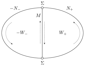
Consider an oriented compact -manifold together with an oriented, properly embedded -manifold , which separates into two pieces . Put differently, is obtained by gluing to along the submanifold . Note that is allowed to have nonempty boundary itself. This decomposition induces a decomposition of the boundaries and ; see Figure 1. From this, we obtain a decomposition of the boundary . We equip then with the orientation .
For a manifold with boundary , define
In our setting, we are interested in the spaces , and . The following result is immediately obtained from the main theorem of [Wal69], as the correction term vanishes as soon as two of the involved subspaces coincide.
Theorem 2.12.
(Novikov-Wall additivity) Let be decomposed as above as the union of and , and suppose that any two among , and are equal. Then
Theorem 2.12 admits a generalization to twisted coefficients. For simplicity, in the twisted setting we shall only state a weaker result which is sufficient for our purposes. Suppose to have a map . With this map, we can construct the local coefficient systems for every , as explained in Example 2.1. The following additivity result holds for the twisted signature.
Proposition 2.13.
Suppose that is decomposed as above as the union of and . Then, for each such that , Novikov-Wall additivity holds for the twisted signature:
2.4. Concordance roots and vanishing results
We generalize the concept of Knotennullstellen [NP17]. After applying this concept to a variation of a well-known chain homotopy argument, we discuss some further properties of these elements.
Let be the subset of Laurent polynomials such that . We abbreviate the Laurent ring with .
Definition 2.14.
An element is a concordance root if there is a polynomial with . Define to be the subset of all elements which are not concordance roots.
Definition 2.14 is a generalization of [NP17, Definition ] to the multivariable case. The key property of non-concordance roots is that they allow us to use a well-known chain homotopy argument [COT03, Proposition 2.10]. The following results are an adaptation of [NP17, Lemma 3.1].
To define the colored (and Alexander) nullity and the colored signature, we will use the bimodules and ; see Definition 3.2 below. A key ingredient, necessary to prove the concordance invariance of these invariants, is the following fact: these modules are not just –right modules, but right -modules where the localisation , inverts all elements of .
Suppose now that is a homomorphism obtained by adding entries. Then, the induced map of group rings fits into the following commutative diagram with the augmentation maps
Recall that, the augmentation map sends a Laurent polynomial to its evaluation . The next lemma follows from considerations of determinants; see cf. [COT03, Proposition 2.4].
Lemma 2.15.
Let be a –module homomorphism with the property that is an isomorphism. Then
is also an isomorphism. Consequently, so is and .
Proof.
See [NP17, Section 3]. ∎
Lemma 2.16.
Let be a non-negative integer, and let lie in . If is a pair of CW-complexes over with for , then both and vanish for .
Proof.
We make the following abbreviations and for the cellular chain complexes of the pairs . For the remainder of the proof, will be an arbitrary integer . The chain complex consists of finitely generated free -modules, and as , it admits a partial contraction, i.e. homomorphisms with
Consider the chain map of chain complexes over , which is induced by tensoring with the augmentation map. Pick a lift of under , which is a homomorphism of -modules such that the following diagram commutes:
Such a lift exists because consists of free modules and the map is surjective. Consider the partial chain map
By construction, and so is also an isomorphism; see Lemma 2.15. We obtain that is a partial chain contraction for and
Now we tensor with either or , which are both right –modules. Here, we use the fact that . Note that is a partial chain contraction for and so . ∎
For the remainder of the section, we collect properties of the set of non-concordance roots. For a prime , define
and . This is the set for which concordance invariance properties and genus bounds are proved in [CF08, Section 7]. The next result shows that the set of non-concordance roots contains .
Proposition 2.17.
The set is contained in .
Proof.
Let and be a polynomial such that . We have to show that . We pick large enough such that all are -roots of unity. The subgroup consisting of the -roots of unity is cyclic. Thus we write for a primitive -root of unity . Define the one variable polynomial . Hence, we have , so is a multiple of the -th cyclotomic polynomial, whose value at equals . It follows that divides and so cannot be equal to . ∎
The following example shows that also contains elements which are not in , but have algebraic coordinates.
Example 2.18.
We claim that the algebraic element is in , but not contained in . The algebraic number , has minimal polynomial and is not a root of unity [NP17, Lemma 2.1]. It follows that is not an element of .
To show that , we prove that any polynomial with has . Consider and note that is a root of . As a consequence divides and is even. It follows that must also be even.
Lemma 2.19.
Let , and be a map. Then is an element of .
Proof.
Let be a polynomial such that , where denotes . Define a polynomial in -variables by the equality . Note that and as , we deduce that . ∎
As shown in the following remark, it is also easy to construct elements which do not belong to and for which our main results will not apply.
Remark 2.20.
Let . A consequence of Lemma 2.19 is that, if belongs to , then all the coefficients belong to . Phrasing it differently, if any of the coefficients of is a concordance root, then itself is a concordance root.
3. Colored signatures and nullities of links
In Section 3.1, we give a definition of the colored signature and nullity of a colored link as twisted invariants of manifolds with boundary. Section 3.2 shows that they coincide with the invariants introduced by Cimasoni-Florens [CF08]; see e.g Proposition 3.4 and Proposition 3.5. Section 3.3 introduces the notion of colored cobordism and presents the statement of Theorem 3.7 which provides obstructions on the possible colored cobordisms that two given colored links can bound. Section 3.4 is devoted to the proof of the theorem. Finally, Section 3.5 provides the applications of Theorem 3.7 and puts it in relation with some previously known results. In particular, we prove the concordance invariance of the signature and nullity and present obstructions on the possible surfaces a colored link can bound in .
3.1. Set-up
This section deals with some preliminaries on colored links and their colored bounding surfaces. Making use of this set-up, we introduce our main invariants: the colored signature and the colored nullity.
Let be a -colored link. We denote the exterior of by and recall that the abelian group is freely generated by the meridians of . Summing the meridians of the same color, we obtain a homomorphism . A colored bounding surface for a colored link is a union of properly embedded, locally flat, compact oriented surfaces with and which only intersect each other transversally in double points. A bounding surface of a link is a union of properly embedded, locally flat, compact, connected and oriented surfaces which only intersect each other transversally in double points, and . Note that we require each to be connected. Forgetting about the colors, a colored bounding surface turns into a bounding surface formed by the union of its connected pieces.
As the surfaces are required to be locally flat, that is they admit tubular neighborhoods. Given a (possibly colored) bounding surface of , we denote by the union of some choice of tubular neighborhoods for its components. We denote then by the exterior of . For the convenience of the reader, we give an argument for the following well-known fact.
Lemma 3.1.
Given a bounding surface , the abelian group is freely generated by the meridians of the components .
Proof.
Pick a small ball around each intersection point of . Note that , where the surface is with little discs removed around the intersection points. The Mayer-Vietoris sequence of with -coefficients gives us
where the ’s arise as the homology for . Applying the Künneth theorem to the products the sequence can be reduced to , where . This concludes the proof of the lemma. ∎
Consequently, there is a canonical homomorphism which restricts to on the link exterior: indeed the inclusion sends the meridians of to the meridians of . Since and are now both spaces over , we can give the following definition.
Definition 3.2.
Let be a colored bounding surface for a -colored link . Given , define the colored signature and the colored nullity by
Viro [Vir09, Theorem 2.A] showed that is independent of the choice of colored bounding surface. For a proof, see also the upcoming paper by Degtyarev, Florens and Lecuona [DFL18]. It is sometimes useful in the following to view as signature defect, which is made possible by the following result, probably well known to the experts.
Proposition 3.3.
If is a colored bounding surface for a -colored link , the untwisted intersection form on is trivial. As a consequence, the signature vanishes and we have .
Proof.
Set so that . Consider the portion of the Mayer-Vietoris sequence associated to the decomposition . It follows that the map is surjective. Since is contained in the boundary of , the natural map is surjective. The statement follows immediately since elements of annihilate the intersection form. ∎
3.2. C-complexes
We recall the multivariable signature and nullity functions introduced by Cimasoni-Florens [CF08] using C-complexes. Our main objective is to show that these invariants coincide with the colored signature and nullity defined in Section 3.1.
A C-complex for a -colored link consists of a collection of Seifert surfaces for the sublinks that intersect only along clasps; see [Coo82, Cim04, CF08] for details. Given such a C-complex and a sequence of ’s, there are generalized Seifert matrices , which extend the usual Seifert matrix [Cim04, CF08]. Note that for all , is equal to . Using this fact, one easily checks that for any in the -dimensional torus, the matrix
is Hermitian. Since this matrix vanishes when one of the coordinates of is equal to , we restrict ourselves to . The multivariable signature is the signature of the Hermitian matrix and the multivariable nullity is , where is the number of connected components of .
We start by proving that , i.e that the colored nullity is equal to the multivariable nullity:
Proposition 3.4.
Let be a -colored link. For every and for any C-complex for , we have the equality .
Proof.
Since the multivariable nullity is independent of the chosen -complex [CF08, Theorem ], pick for which there is at least one clasp between each pairs of surfaces and , so that in particular . Note that this is possible thanks to [Cim04, Lemma ]. Using [CF08, Corollary 3.6] the Alexander module admits a square presentation matrix given by . Tensoring with we deduce that presents . Using Lemma 2.6, we obtain that and consequently also presents . The result follows immediately. ∎
We conclude by showing that the colored signature coincides with the multivariable signature of Cimasoni-Florens [CF08].
Proposition 3.5.
If is a -colored link , then , i.e. the colored signature is equal to the multivariable signature.
Proof.
Since the colored signature is independent of the choice of a colored bounding surface, we can take to be a push-in of a C-complex in the -ball; see [CFT16, Section 3.1] for a precise description. By [CFT16, Theorem ], the intersection pairing is represented by . Since we wish to show that the intersection pairing is represented by , the theorem will follow if we manage to produce the following commutative diagram
| (1) |
Further assuming to be totally connected implies that vanishes for , and is a finitely generated free -module for [CFT16, Section and Proposition ].
Consider the following diagram below, where homology groups and tensor products without coefficients are over . Applying the universal coefficient spectral sequence, as described in Propositions 2.3 and 2.5, the first three vertical maps in the following commutative diagram are isomorphisms
The last vertical map is an isomorphism since is finitely generated and free. Considering the adjoint, we precisely obtain the diagram of Equation (1). ∎
3.3. The genus bound
For elements , the multivariable signature and nullity are known to give lower bounds on the genus of colored bounding surfaces [CF08, Theorem 7.2]. In this section we prove a more general result for surfaces in . As corollaries, we extend the concordance invariance results of [CF08, Theorem 7.1] and generalize the lower bounds of [CF08, Theorem 7.2].
Definition 3.6.
A colored cobordism between two -colored links and is a collection of properly embedded locally flat surfaces in that have the following properties: the surfaces only intersect each other in double points, each surface has boundary , and each connected component of has a boundary both in and in . We say that has components if the disjoint union of the surfaces has connected components.
The main result of this section is the following lower bound.
Theorem 3.7.
If is a colored cobordism between two -colored links and with double points, then
for all .
Remark 3.8.
The right-hand side of the inequality can equivalently be expressed in terms of the first Betti number or of the genus of the surfaces. Suppose that is an -component link, is an -component link, and that the cobordism has components (in the sense of Definition 3.6). Then, we have the following equalities:
For this reason, we will usually refer to the inequality of Theorem 3.7 as a genus bound, even if the genus does not appear explicitly in the formula.
3.4. Proof of the main theorem
We proceed towards the proof of Theorem 3.7, starting with a series of preliminary results.
First, we describe the Euler characteristic of the exterior of a colored cobordism in in terms of the Euler characteristic of the surfaces .
Lemma 3.9.
Suppose is a -colored cobordism between two colored links and with double points. Then the Euler characteristic of is given by
Proof.
First, we prove that . Consider the decomposition and set . Using the decomposition formula for the Euler characteristic yields . As the Euler characteristic of a -manifold with toroidal boundary vanishes, . Since also vanishes, the claim follows. Now note that is homotopy equivalent to the union . Recall that the surfaces intersect each other in points. We apply again the decomposition formula for and obtain
∎
By Lemma 3.1, one observes that is freely generated by the meridians of . Consequently, there is a homomorphism that extends the maps on and .
Next, we observe that with coefficients, the boundary of behaves as the disjoint union of the link exteriors and .
Lemma 3.10.
The inclusion of into induces an isomorphism
for all .
Proof.
The next lemma provides some information on the twisted homology of .
Lemma 3.11.
If is a -colored cobordism between and and , then
-
(1)
and ,
-
(2)
for .
Proof.
As and are both connected, there is an isomorphism . Since the inclusion takes meridians to meridians, is surjective. Combining these facts, , so that Lemma 2.16 gives for . It follows from the long exact sequence of the pair that the inclusion induced map is surjective, and thus . Repeating the argument for , the first statement is proven.
Since the inclusion of into factors through , an analogous argument shows that for . Lemma 2.4 now implies that for .
Note that the entries of are different from . This implies that the vector space vanishes by its description as a quotient [HS97, Section VI.3]. ∎
We conclude this section with a dimension count, which will prove itself useful to bound the twisted signature of .
Lemma 3.12.
Denote by the map induced by the inclusion. Then, for , we have
Proof.
We are now ready to conclude the proof of Theorem 3.7.
Proof of Theorem 3.7.
We start by proving the following inequality:
As in Lemma 3.12, we use to denote the map . Since the twisted intersection form descends to a pairing on , an application of Lemma 3.12 yields
| (2) |
Now, thanks to Lemma 3.11, we have , and using Lemma 3.10, one gets . Using these last two identities, Equation (2) can be rewritten as
The desired inequality is now obtained by using Lemma 3.11 to bound above both by and .
With the inequality above, Theorem 3.7 will follow from Lemma 3.9 once we have established that
Pick a colored bounding surface for . Thanks to Proposition 3.3, we have . One can now form the surface with singularities . Using an orientation-preserving diffeomorphism between and , the surface is sent to a colored bounding surface for . Its exterior is clearly homeomorphic to . Once again thanks to Proposition 3.3, we have . Since , Proposition 2.13 implies that Novikov additivity holds for the twisted signature, yielding
Summarizing, we have shown that . Combining this with the inequality of Equation (2) concludes the proof of Theorem 3.7. ∎
3.5. Applications of the genus bound
We will give two applications of Theorem 3.7. First, we show that the colored signature and nullity are concordance invariants, see Corollary 3.13, then we study the genus of colored bounding surfaces in Corollary 3.15.
Two -colored links and are concordant if there exists a -colored cobordism between and which has no intersection points and consists exclusively of annuli.
Corollary 3.13.
If and are two colored links that are concordant, then
for all .
Proof.
We apply Theorem 3.7 to the case where each is a union of annuli and there are no double points. The result follows as all the terms in the right-hand side of the inequality are zero. ∎
Remark 3.14.
Note that Corollary 3.13 will be significantly improved upon in Section 5: the signature and nullity will be shown to be invariant under -solvable cobordisms.
Using to denote the first Betti number of a surface , an application of Theorem 3.7 also gives the inequality below.
Corollary 3.15.
Let be a colored bounding surface for , and suppose that has components and intersection points. Then, for all , we have
Proof.
Remove small -balls in the interior of on each component of . With small enough balls, will intersect the boundary spheres in unknots. Tubing the boundary spheres together, we have constructed a -colored cobordism with components between and a -colored unlink of components. Thanks to the results of Section 3.2, we can compute the signature and nullity of using C-complexes [CF08, Section 2]. We pick a disjoint union of disks as a C-complex. The resulting generalized Seifert matrices are empty, yielding and for all . Using Theorem 3.7 and Remark 3.8, we get
Now, if is any of the components of , the corresponding component of is obtained from by removing a small disk, so that . Summing over all the components, we get , whence the desired formula. ∎
The next example discusses the (non)-sharpness of the bound of Corollary 3.15.
Example 3.16.
We start with an example where the bound is sharp. Consider the -colored Hopf link (with any orientation). The oriented link bounds an annulus in , and we compute and . If we push into the –ball, we obtain a bounding surface . The inequality of Corollary 3.15 is sharp:
Although it is easy to construct examples where this inequality is not sharp, we claim that the defect can in fact be arbitrarily large: pick a family of knots such that has the Seifert matrix of a slice knot, and topological –genus (such knots exist thanks to [Cha08, Theorem 1.3]). Now consider , where we tie the knot into in a small –ball disjoint from . The signature and the nullity do not change, but we have , concluding the proof of the claim.
Instead, if we pick each knot to be topologically slice, but with smooth –genus (such knots exist [Tan98, Remark 1.2]), then the provide a family of knots where the inequality is sharp in the topological category, but not in the smooth category.
We now compare Corollary 3.15 with previous results.
Remark 3.17.
Corollary 3.15 is a generalization of [CF08, Theorem 7.2]. In that paper, it is proven in the smooth setting and requires to be in the set , which is strictly smaller as ; see Example 2.4. Since all surfaces are assumed to be connected, appears instead of in their formula.
We can also recover a previous result [Pow17, Theorem 1.4] bounding the -genus of a -colored link with components. Consider disjoint surfaces in bounding . Indeed, is a -colored bounding surface for , and applying Corollary 3.15, we get
for . The result follows by passing to the minimum over all such collections of surfaces and observing that is dense in .
Finally, note that Viro proves inequalities similar to Corollary 3.15 in any odd dimension. In particular, for links in he obtains and [Vir09, Theorem 4.C]. Reworking his equations leads to the inequality
which is slightly weaker than Corollary 3.15. The interested reader will note that while Viro essentially obtains his results for all , his methods are quite different from the chain homotopy argument we rely on, see [Vir09, Appendix C].
4. Plumbed –manifolds and surfaces in the –ball
In this section, we review plumbed -manifolds and prove a vanishing result for their signature defect. This result is a key step in the proof of Theorem 1.5 (which is concerned with the invariance of the signature and nullity under -solvable cobordisms). In Section 4.1, we show this vanishing result in the case of products of a closed surface with . To do so, we apply a product formula for the Atiyah-Patodi-Singer rho invariant, and pass from the smooth to the topological setting by using a bordism argument. In Section 4.2, we introduce the framework of plumbed -manifolds and prove the main result, which is contained in Proposition 4.10. This proposition shows that the signature defect of a -manifold vanishes if its boundary is a so-called “balanced” plumbed -manifold. Finally, in Section 4.3 we describe how plumbed -manifolds arise naturally from surfaces intersecting transversally in the -ball, and we perform a homological computation which is needed in Section 5.
4.1. The rho invariant of a product
We consider the rho invariant , a real number, in the special case of being a smooth, odd dimensional manifold with a homomorphism [APS75]. The definition of the rho invariant requires spectral analysis of elliptic differential operators on a manifold, and we will not attempt to recall it. Instead we state the following properties of , which will be sufficient for the purposes of this article.
Proposition 4.1.
-
(1)
If is a smooth -manifold together with a homomorphism , then .
-
(2)
If is a closed smooth -manifold with a homomorphism , and comes with a homomorphism , then
In particular, if is odd.
Proof.
The first result is the specialization to our setting of the Atiyah-Patodi-Singer index theorem [APS75, Theorem 2.4]. The formula in the second statement follows from a direct computation combined with the classical Atiyah-Singer theorem. Both results can be found in [Neu79, Theorem 1.2, (iii) and (v)], where it has to be observed that the invariant considered by the author differs from the rho invariant by a sign and that (this follows from (1) since has no boundary, or alternatively from the Hirzebruch signature formula; see Remark 2.9). The last claim follows immediately from the fact that the ordinary signature of a closed manifold is non-trivial only in dimension . ∎
We restrict further to manifolds with a homomorphism . Since one-dimensional representations of factoring through are in bijection with values , we will denote by the rho invariant corresponding to the representation given by the composition
Using Proposition 4.1, we prove the following lemma.
Lemma 4.2.
If is a closed oriented connected surface and is a homomorphism, then for all .
Proof.
The following corollary is nearly immediate.
Corollary 4.3.
Let be a set of closed oriented connected surfaces. If is a -manifold over with boundary
then .
Proof.
Since Proposition 4.1 required the cobounding manifold to be smooth, one might worry about Corollary 4.3 only holding for smooth -manifolds . The following remark deals with this issue.
Remark 4.4.
Let be a topological -manifold bounding . The bordism groups are computed in both the topological case and the smooth case by . Thus, if bounds topologically, then there also exists a smooth filling , for which the rho invariant computation gives . By Corollary 2.11, the difference between twisted and ordinary signature is the same for two -manifolds filling the same over , so we conclude that is also zero as desired.
4.2. Plumbings and their signature defect
After reviewing the definition of a plumbed -manifold, we use the rho invariant to observe that if a -manifold admits a balanced plumbed -manifold as its boundary, then its signature defect vanishes; see Proposition 4.10. Classical references on plumbed -manifolds include [Neu81, HNK71]. See also [BFP16] for their use in our context.
We begin by setting up notation.
Construction 4.5.
Let be an unoriented graph with no loops. The set is the set of oriented edges, and and are the source and the target maps. The involution sends an oriented edge to the corresponding edge with the opposite orientation; see e.g. [Ser80, Section I.2]. The graph is unoriented in the sense that for each edge, the set also contains the edge with the opposite orientation. We shall sometimes also denote by . Assume that the set of vertices consists of oriented, connected and compact surfaces and that the edges are labeled by weights .
For each edge , we choose an embedded disc in such a way that no two discs intersect. We then remove these discs, by defining for each surface the complement
We define the plumbed -manifold as
where, for all the identifications are given by
| (3) | ||||
Since these identifications make use of orientation reversing homeomorphisms, the -manifold carries an orientation that extends the orientation of each .
Remark 4.6.
The orientation is the one obtained by considering the circle as a boundary component of . This is the opposite of the one induced by the boundary of the removed disk. In the general context of plumbing disk bundles, one trivializes over the removed disks, which causes the two formulas to flip; see e.g. [HNK71, Chapter 8 p. 67].
The boundary of a plumbed -manifold is a union of tori and the components correspond to the boundary components of the surfaces . By construction, the boundary components come with the product structure . We define the homology class in .
In order to describe the kernel , we introduce some more notation: for each surface with boundary, label its boundary components and accordingly their meridians and longitudes . We have the equality . The vertices of our graph are surfaces. So, for each edge , the expression denotes a surface and denotes the meridian of –th boundary torus of . The following lemma describes the kernel of the inclusion , which will be useful for our applications of Novikov-Wall additivity.
Lemma 4.7.
The kernel of the inclusion induced map is freely generated by the elements
for varying over the elements in with and .
Proof.
From the construction of , we see that for every edge there is a torus which is identified with . We denote this torus by . Hence, .
Now pick an orientation on the edges, i.e. for every , exactly one of the edges and is an element of . From the construction of , we obtain a Mayer-Vietoris sequence
where denote the maps induced by the inclusions of into and respectively. For each , the inclusion factors through the space . Consequently, we have the commutative diagram of inclusion induced maps
yielding We shall now restrict our attention to those surfaces with , and prove that both and belong to . As is connected, all elements for are equal in , so the elements are in and a fortiori in . Next, we check that an element of the form is sent by to the image of . Note that , so that we have the relation in . We thus obtain
and the claim reduces to checking that this element is in the image of . Consider the class . We have and, by the gluing map given in Construction 4.5, . As a result, the difference is indeed in the image of , and so is in .
Note that the elements in the statement of the lemma span a subspace , whose dimension is the number of boundary components of , i.e. it is half the dimension of the space . By the half lives, half dies principle [Lic97, Lemma 8.15], the kernel has the same dimension as and so coincides with . ∎
Definition 4.8.
Let a graph with a label function . For denote by the set of all edges between and . We call the integer the total weight of the pair of distinct vertices . The graph is called balanced if for all such pairs .
From now on, assume that our plumbed -manifold comes with a homomorphism . We call such a homomorphism meridional if, for each constituting piece with , the restriction of to sends the class of to one of the canonical generators of . Moreover, in the next two results we will restrict our attention to plumbings of closed surfaces.
The next lemma shows that if is balanced, then is cobordant to a disjoint union of trivial surface bundles, where the cobordism has vanishing signature defect.
Lemma 4.9.
Let be a balanced graph with vertices closed connected surfaces. Suppose that is a meridional homomorphism. Then there exists a smooth -manifold over such that:
-
(1)
the boundary of is a disjoint union
where every is a closed oriented surface;
-
(2)
the restriction is meridional;
-
(3)
for all .
Proof.
Instead of proving the statement directly, we prove the following: if is nonempty, then there exists a balanced graph with the same number of vertices and fewer edges than , such that there exists a manifold over with , which induces a meridional homomorphism on and such that for all .
The original statement can be recovered as follows: iterate the above to obtain a sequence of graphs such that the set of edges of is empty. Consequently, . We then glue the -manifolds together: . We get as required and by Novikov additivity .
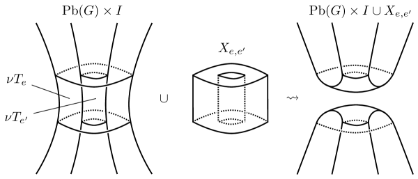
Now we proceed with the proof of the modified statement. Recall from Construction 4.5 that to each edge corresponds the embedded torus . The complement of all of these tori is diffeomorphic to . In order to produce the desired -manifold , our aim is to attach a to the trivial bordism .
Given two vertices , we write as in Definition 4.8. Pick two vertices such that is nonempty. As the graph is balanced, this implies we can also pick two edges such that and . Now set . Consider the corresponding tori and , with oriented neighborhoods , . We attach to along its vertical boundaries through a homeomorphism given by the following formulas:
The induced orientations on are such that the above map is orientation-reversing. As a consequence, the orientations of and extend to the resulting -manifold
Let the images of the meridians of and under the map . Recalling the construction of given in (3), we see that the induced maps to on and are given by
The difference in the sign of the image is a consequence of the fact that the edges had opposite signs. This allows us to define a map which glues with the map , i.e. the following diagram commutes:
By making an additional choice of a splitting of the Mayer-Vietoris sequence
we obtain a map which extends and on and .
The boundary of has two components. The bottom boundary is . The effect of adding on the top boundary is that of cutting along and and gluing together the boundary component to , and glueing to . Let be the result of –surgery along and in , and define similarly. The top boundary inherits a plumbed structure along a graph obtained from by replacing the vertices and with and , and by removing the edges and .
We have verified that fulfills the first statement. To conclude the proof of the proposition, it remains to prove that . This is a consequence of the following claim.
Claim.
The twisted and untwisted signature of and vanish and Novikov-Wall additivity holds when gluing these two pieces together.
To prove that the signatures vanish, note that both spaces are -manifolds with the property that the inclusions of the boundary and surject. This implies that both the twisted and untwisted intersection forms vanish. In particular, the twisted and untwisted signatures of and are zero.
Next, we consider Novikov-Wall additivity. We are gluing to along . In the notations of Section 2.3, we have and . The boundary of the gluing region is given by the four tori
We shall prove that and agree, so that the hypotheses of the Novikov-Wall additivity theorem are satisfied (recall Theorem 2.12) .
Observing the gluing maps above, we see that the vector space has basis
| (4) |
In order to describe , observe that inherits a plumbed structure from . It has the same surfaces as vertex set with and replaced by and . Its set of edges is obtained by removing and from the set of edges of . Note that and we can use Lemma 4.7 to obtain a basis for . The difference of meridians gives the basis elements . The surface has boundary , so that further elements of the basis are given by
where the equality follows from the fact that is balanced. The analogous statements holds for the other surface . Consequently, the vector space admits the same basis (4) as , and hence they coincide. In particular, Theorem 2.12 applies, and the untwisted signature is additive.
For the twisted signature, thanks to Proposition 2.13, it is enough to prove that the twisted homology vanishes for . This happens exactly if the induced -representation is nontrivial. This is the case, because is meridional and the entries of are taken to be different from . Consequently, the signature defect is additive and so
∎
Using Lemma 4.9, we can prove our main result about plumbed manifolds.
Proposition 4.10.
Let be a balanced graph with vertices closed connected surfaces . Suppose that is a meridional homomorphism and that bounds a -manifold over . Then, for all ,
Proof.
Since the graph is balanced, Lemma 4.9 produces closed surfaces and a -manifold over whose signature defect vanishes, with boundary
One can now define . Since the boundary of consists of a disjoint union of , Corollary 4.3 guaranties that . As we are gluing along a full boundary component, Novikov additivity holds for both the twisted and untwisted signature, leading to . Since we know that both and vanish, also vanishes. ∎
4.3. Surfaces in the –ball
In the remainder of the paper, plumbed -manifolds will mostly appear as boundaries of tubular neighborhoods of collections of surfaces in the -ball.
We observe that the exterior of a bounding surface contains a plumbed -manifold in its boundary.
Definition 4.11.
The intersection graph of a bounding surface has the vertex set . The set of edges consists of triples where is an intersection point between the components . The maps are defined on by
Moreover, we assign a weight to each edge corresponding to the sign of the intersection at the point .
Our interest in plumbed -manifolds essentially lies in the next example, which is only balanced if the link has pairwise vanishing linking numbers.
Example 4.12.
Let be a bounding surface for a link . The boundary of the exterior decomposes into . Plumbing the trivialized disk bundles by the intersection graph of describes a neighborhood of . In this model, the surfaces are recovered as the zero sections [HNK71, Chapter 8]. As consequence, we see that is diffeomorphic to , where is the intersection graph of .
Let be a bounding surface for a link , and let be the sublink given by , for . Denote as usual the exterior of by . Recall from Example 4.12 that , where is a plumbed -manifold. Enumerate the components of and denote their meridians by for , where is the number of components of . Define the linking number between two disjoint sublinks by
where the sum runs over the link components of and , and set for all . The following computation will turn out to be useful when applying Novikov-Wall additivity.
Lemma 4.13.
The vector space is generated by the elements of the form
Proof.
Consider the surface for an edge and the corresponding sublink , whose first component has meridian . Applying Lemma 4.7, the component gives rise to the basis vectors
The result follows by observing that
∎
5. Invariance by –solvable cobordisms
The aim of this section is to prove that the multivariable signature and nullity are invariant under -solvable cobordism. Sections 5.1 and 5.2 respectively review the notion of -cobordisms and -solvable cobordisms. Section 5.3 tackles the invariance of the nullity. Section 5.4 is concerned with invariance of the signature. Finally, Section 5.5 proves some technical results which are used in Sections 5.3 and 5.4
5.1. –cobordisms
In this section, we review the definition of an -cobordisms between 3-manifolds and prove some elementary properties following [Cha14].
A cobordism between two connected -manifolds with a preferred orientation-preserving diffeomorphism is a compact connected -manifold with a decomposition . We will often suppress from the notation. A cobordism is an -cobordism if additionally the inclusions of and into induce isomorphisms .
We start by recalling some immediate facts about -cobordisms.
Lemma 5.1.
If is an -cobordism, then the following statements hold:
-
(1)
for all .
-
(2)
The groups and are isomorphic and free abelian.
-
(3)
Denote by the map induced by the inclusion. There exists a unique map such that
is commutative. The map is an isomorphism.
Proof.
Since the first two assertions can be found in [Cha14, Lemma 2.20], we only show here the third one here. As a first step, we show that the map arising from the long exact sequence of the triple is an injection. To prove this, consider the diagram
where exc denotes excision. The upper square clearly commutes, while the pentagon commutes by [Bre93, Section , Problem ]. Since is an -cobordism, the uppermost horizontal map is an isomorphism. Consequently, the map is an isomorphism and therefore so is the map . Exactness now implies that is injective.
As a second step, we show existence and uniqueness of . The portion
of the long exact sequence of the pair produces the short exact sequence in the top row of the following commutative diagram:
Since is an -cobordism, the group vanishes. Consequently, given , the composition is zero and so, by exactness, there exists such that . We therefore define . As is injective, is well-defined. By construction .
Next, we show that is an isomorphism. Injectivity is immediate from the diagram above and the fact that is injective. As , we obtain the following commutative diagram
which shows the surjectivity of . ∎
Given an -cobordism with a map , we shall often consider homology and cohomology with twisted coefficients in either or (for ). In both cases, we denote the underlying fields or by , so that the twisted (co-)homology groups are vector spaces over . As in Section 2.1, for a pair we denote by the rank of and by the dimension of . We conclude this subsection with a consequence of Lemma 2.16.
Lemma 5.2.
Let be an -cobordism equipped with a homomorphism . Then both and vanish for and for all . In particular, equals .
5.2. –solvable cobordisms
We review here the notion of -solvable cobordism as defined in [Cha14]. For simplicity, we avoid discussing -solvability and -solvability, referring to [Cha14] for a more general treatment.
In the following paragraphs, given an -cobordism , we use as a shorthand for and use to denote the -valued intersection form on . Recall the following definition from [Cha14, Definition 2.8], which extends the definition of solvability from Cochran-Orr-Teichner’s work [COT03] to a relative notion.
Definition 5.3.
An -cobordism is a -solvable cobordism if there exists a submodule together with homology classes that satisfy the following properties:
-
(1)
the intersection form vanishes on ;
-
(2)
the image of under the composition has rank ;
-
(3)
the images of the elements fulfill the relation for each ;
We refer to as a –lagrangian, and to as its –dual.
Remark 5.4.
Suppose that is a –solvable cobordism with –langrangian . Then the images of the ’s in span a free submodule of rank , since they are dual to the ’s.
For further reference, we make note of the following result, whose proof is outlined in [Cha14, Proof of Theorem ].
Proposition 5.5.
The signature of a –solvable cobordism vanishes.
Proof.
Let be the image of the –lagrangian under . Let be the isomorphism of Lemma 5.1. The subspace is Lagrangian for the non-singular intersection pairing of . Consequently, the signature of vanishes. ∎
The next definition is an adaptation to the colored framework of the definition given by Cha [Cha14]. Recall that the boundary of a link exterior inherits a product structure by longitudes and meridians, which is well-defined up to isotopy. A bijection of the link components of two links induces an orientation-preserving diffeomorphism preserving the product structures, which is unique up to isotopy.
Definition 5.6.
Two colored links are -solvable cobordant if there exists a bijection between the components of and of which preserves the colors and there is a -solvable cobordism .
Example 5.7.
Suppose and are concordant, and let be a concordance exterior. Then is a homology cobordism, which is a –solvable cobordism since .
Recall from Section 3.1 that the exterior of a -colored link is equipped with a homomorphism . A -solvable cobordism between two colored links and fits into the commutative diagram
| (5) |
where is the isomorphism that sends the meridian of a component of to the meridian of the corresponding component of . We recall that the linking number between two disjoint sublinks is defined as the sum over the linking numbers of all their respective components (see Section 4.3).
Lemma 5.8.
Let and be two –cobordant oriented links. If is a cobordism between them, then
for each pair of components of . In particular, if and are concordant as -colored links, then for each pair of colors .
Proof.
The abelian group is freely generated by the meridians of , so that every element has a well defined coordinate corresponding to the meridian of . By definition, the linking number is the coordinate of the longitude of . Let be the longitude of . Since the longitudes are glued together, we have in Diagram (5), and hence by commutativity of the diagram. As the map sends meridians to meridians, it preserves the coordinates, and hence . The proof of the first statement is concluded by observing that is by definition the linking number between and . The equality concerning -colored links follows immediately from the fact that the cobordism preserves the colors. ∎
Given a -cobordism with a map , the homomorphism and the canonical map induce homomorphisms and , where stands either for or for . Also, we write for the -valued intersection form on .
The invariance of the signature and nullity will hinge on the following two results whose proof we delay until Section 5.5.
Proposition 5.9.
Let be either or , with . Let be an –solvable cobordism over with –lagrangian . Then both subspaces
have dimension . Furthermore, they satisfy the following two properties:
-
(1)
the intersection form vanishes on .
-
(2)
.
Proof.
See Proposition 5.15. ∎
When , we shall often drop the from the notation of the Lagrangian and simply write . The next proposition provides a lower bound on the dimension of .
Proposition 5.10.
Let be two -colored links that are –solvable cobordant via with –lagrangian . Then
Proof.
See Proposition 5.18.∎
Using the two propositions above, we can now prove the invariance of the nullity and signature under 0.5-solvable cobordism.
5.3. Nullities and –solvability
The next result states the invariance of the multivariable nullity and Alexander nullity under -solvable cobordisms.
Proposition 5.11.
Let be either or , with . If is a –solvable cobordism, then the -vector spaces and have the same dimension. In particular, if and are -solvable cobordant links, then and for all .
Proof.
Consider the exact sequence of the pair in which coefficients are understood:
We use to denote the Betti numbers with -coefficients. Since the Euler characteristic of the sequence is zero and since duality implies that , the proposition boils down to showing that and have the same dimension. This is proved in Lemma 5.12 below. ∎
We are indebted to Christopher Davis for suggesting that we prove the following key lemma.
Lemma 5.12.
Let be either or , with . The images of the two maps
have the same dimension over .
Proof.
Consider the three following intersection pairings:
These pairings are related as follows. First, observe that the map induced by the inclusion factors as , where the map is also induced by the inclusion. We introduce the same notation for , resulting in a map . Consider the following diagram:
The left triangle and right square are clearly commutative, while the middle square commutes thanks to [Bre93, Section 6.9 Exercise 3]. It now follows that for in and in , we obtain
| (6) | ||||
We introduce one last piece of notation. By Proposition 5.9, the subspaces , , and all have dimension .
Now we construct a subspace
by constructing the elements . Pick a basis . Since the dimension of is , the elements form a basis of . Therefore, the assignment defines a map . Since is a field, is a direct summand and consequently extends to an element . The element corresponds to under the isomorphism given by the adjoint of . This is an isomorphism, since the pairing is non-singular.
Consequently, the space is freely generated by elements that satisfy
| (7) |
Completely analogously, we can define a subspace of with a basis given by . Summarizing, we now have subspaces and of and subspaces and of .
Claim.
The subspaces and intersect trivially.
To prove this, start with and an arbitrary in . There is an in such that . Similarly, since lies in , there is a in such that . Using (6), we now have
| (8) |
where the last equality is due to the fact that . Since also lies in , we can write . Combine Equation (8) with the property of the ’s in Equation (7) to deduce that for each . This implies that , concluding the proof of the claim.
Using the claim it now makes sense to consider the direct sum . Since and both have dimension at least , we conclude that the dimension of must at least be . Using Lemma 5.2, we see that the dimension of is equal to . Combining these observations and repeating them for , we deduce that
| (9) | ||||
| (10) |
Recall that and denote respectively the maps from to and . Since, by definition, the subspaces and are images of under and , we deduce that they are subspaces of and .
By (9), , and the same for . Since we just argued that , and , it follows that
Since we wish to show that and since and have dimension by Equation (10), it only remains to prove the following claim:
Claim.
.
Since and are freely generated by the and , there is an isomorphism obtained by mapping the to the . The claim will follow if we show that restricts to an isomorphism from to .
First, we check that the map restricts to a map . So assume that lies in . By definition is equal to , which clearly lies in . Consequently we have to show that lies in . Since lies in , there is a in such that . Now consider the element of : to show that lies in , it is enough to show that lies in . Consequently, we consider the submodule
and start by verifying that . Recall that the ’s form a basis of and so it is enough to show that vanishes for each . This follows successively by using the definition of , the definition of the ’s in (7), and the property in (6):
Note that , since by the first claim above. Consequently, the vector belongs to and thus to . Since was defined as , we deduce that must also lie in , as desired. We showed that restricts to a map .
Now, by interchanging the roles of and in the argument above, we learn that the inverse restricts to a map . This restriction is the inverse of and thus the latter is an isomorphism. This concludes the proof of the last claim and thus of the proposition. ∎
5.4. Signatures and –solvability
We prove that -solvable cobordant links have the same multivariable signatures, concluding the proof of Theorem 1.5 from the introduction.
Theorem 5.13.
If two -colored links and are -solvable cobordant, then, for all , we have
Proof.
Let be colored bounding surfaces for and respectively, with the additional requirement that they have only a single component per color. We denote by and their respective exteriors and by the link exteriors. Setting as usual , we see that the boundary decomposes into . An analogous decomposition holds for . Let be a 0.5-solvable cobordism, with , where identifies with . We consider the -manifold
which has boundary , where is a disjoint union of tori.

By diagram (5), the coefficient systems on the link exteriors and extend over and thus over . We shall now compute in two different ways.
Claim.
The claim is proved by a double application of Novikov-Wall additivity, each time both for the twisted and untwisted signature: first we prove additivity for the gluing along of the two manifolds and , and then for the gluing along of with . In both cases the boundary of the gluing region is , which is identified with through . As , the hypotheses of Proposition 2.13 are satisfied in the two cases, and twisted additivity holds. Let
In the gluing along , the three spaces to be considered for checking the hypotheses of Theorem 2.12 are , , and in the same order as in the statement. In the second gluing, it is , , and . We show now that and , so that the hypotheses are satisfied in both cases and additivity for the untwisted signature also holds. The space is described by Lemma 4.13. The space is also described by Lemma 4.13 as a subspace of . By Lemma 5.8, the two links have the same pairwise linking numbers. Since we assumed that and have exactly one component for each color, the two vector spaces are seen to coincide under the identification between and . The spaces and also only depend on the linking numbers, and once again they coincide thanks to Lemma 5.8. Hence, Novikov-Wall additivity holds both for the twisted and untwisted signature, and the claim is verified.
Thanks to Proposition 3.3, we have and . The claim gets hence rewritten as
We will now show that both signature defects and are actually , from which the conclusion follows.
By Proposition 5.5, the ordinary signature of vanishes. Invoking Proposition 5.10, there exists a Lagrangian for the nonsingular intersection form on and thus the twisted signature of must also vanish, so that .
To conclude the proof, it only remains to show that . Recall that , where is a disjoint union of tori. We have seen in Example 4.12 that can be described as a plumbing of the components of along its intersection graph. In particular, the total weight between two vertices is given by
Similarly, the manifold is obtained by plumbing the surfaces , along the negative of the intersection graph of (i.e. with its labels reversed), so that
The cobordism gives a bijection between the components of and those of , that induces homeomorphisms along which we can glue the components of and in order to get closed oriented surfaces (). Then can be described as a plumbed -manifold, whose plumbing graph has the surfaces ’s as vertices, and edges . In particular, for each pair of vertices, we have
as the linking numbers of and match up. This means that the plumbed -manifold is balanced, and Proposition 4.10 now implies that as desired. ∎
5.5. The proof of Proposition 5.9 and Proposition 5.10
At this stage, we have proved Theorem 1.5 skipping the proofs of Proposition 5.9 and Proposition 5.10. The aim of this last subsection is to prove these technical results, starting with some preliminary lemmas.
We consider the following set-up: let be an –bordism over , that is the cobordism is equipped with a commutative diagram
We abbreviate by . The composition and the canonical inclusion induce homomorphisms
where stands for or .
We start with a proposition whose proof is inspired by an argument of Cochran-Orr-Teichner [COT03, Proposition 4.3].
Proposition 5.14.
Let be either or , with . Let be an –cobordism over . Let be elements whose projections are linearly independent. Then, the elements are linearly independent in .
Proof.
First, we establish suitable CW-structures on the manifolds and .
Claim.
The pair admits a finite CW-structure (up to homotopy), that is there exists a finite CW-complexes and a subcomplex with a diagram
where the horizontal maps are homotopy equivalences and the diagram commutes up to homotopy. Furthermore, we can pick to be a –dimensional complex and to be –dimensional.
Note that is a –manifold with nonempty boundary, so it admits a smooth structure and one can find a –dimensional CW-structure from a Morse function without critical points of index ; see [Mil65, Theorem 8.1 (Index 0)].
Since is a –manifold with boundary, Poincaré duality shows that the homology group vanishes for (this involves an explicit computation of ). The –manifold admits a finite CW-structure, since it is an absolute neighbourhood retract [Han51, Theorem 3.3]; see [Wes77]. Using a result of Wall [Wal66, Corollary 5.1], these two facts imply that there exists a –dimensional CW-structure .
Use the inverse of the homotopy equivalence to obtain a map and arrange to be a subcomplex by replacing with the mapping cylinder of . Since was a –complex, is still –dimensional.
Before we proceed with the next claim, note that the commutativity up to homotopy is exactly the ingredient needed to construct a map between the cylinders of the inclusions . Consequently, the relative homology groups of , and agree.
Claim.
Without increasing the dimensions of , we may assume that there exists a subcomplex disjoint from with
First, we realize the homology classes geometrically: For each class , there exists a closed oriented surface together with a map such that [Tho54, Théorème III.3], where is the abelian cover of corresponding to the composition . Use the inverse of the homotopy to obtain maps . Consider the space on which acts by multiplication on the first factor. Define the –equivariant map
We now think of as a subspace of the mapping cylinder . Note that the quotient , and is a subcomplex, which is also disjoint from . Replace by , which is a –dimensional complex, since the surfaces are –dimensional. The subcomplex has homology , which is freely generated by the . This concludes the proof of the claim.
Having constructed suitable CW-structures on and , we now proceed with the proof. Observe that the following quotient map is a chain isomorphism
| (11) |
where the coefficient system is either or . In particular, the assumption on the projections precisely means that the map is injective. Similarly, our goal is to show that the induced map is injective. Indeed, this map sends the –basis of to the elements .
In order to establish injectivity, consider the following exact sequence of the triple with coefficients:
| (12) |
Note that Lemma 5.2 shows that the homology group vanishes. As we shall see below, the proposition reduces to the following claim.
Claim.
The homology group vanishes.
Consider the long exact sequence (12) above for . Recall that is injective by assumption, and vanishes since is an –bordism. This shows that . Since the CW-structure of has no –cells, the (cellular) chain module . From these two facts, deduce that the boundary operator is injective. Now we relate this observation to the case : is a homomorphism between free modules, and since is injective, we deduce that is injective by Lemma 2.15. This implies the claim that .
We now conclude the proof of the proposition. Using the claim and (12), we deduce that is injective. As we mentioned above, this shows that the are linearly independent and thus the proof is concluded. ∎
The next proposition was Proposition 5.9 above.
Proposition 5.15.
Let and let be either or . Let be an –cobordism over with –langrangian . Then the subspaces
have dimension . Furthermore, the intersection form vanishes on .
Proof.
Denote the –duals of by . Denote by , and consider the map , which is induced by the augmentation map . By definition of a –cobordism, the images of the elements fulfill the relation for each . This relation descends to the pairing
that sends to where is the relative class of , that is the image of under the map induced by the canonical inclusion. Consequently, the elements are linearly independent. Now apply Proposition 5.14 to the elements to see that the ’s are linearly independent. Since sends , the elements are linearly independent as well. ∎
The final step is to prove Proposition 5.10, that is the inequality
for cobordisms between link exteriors. We start with two preliminary lemmas involving twisted Betti numbers.
Lemma 5.16.
If two -colored links and are -cobordant via , then for and for all we have
Proof.
We start by establishing two preliminary equalities. As is a link exterior, its Euler characteristic vanishes. Since and vanish and since , we obtain
| (13) |
and similarly for . Arguing as in Lemma 3.10, one deduces that . Using (13), we then see that equals and therefore
| (14) |
We now prove the first equality displayed in the lemma (the proof of the second is identical). Lemma 5.2 shows that both modules and vanish. Consider the long exact sequence of the triple
and deduce that . Since the alternating sum of dimensions of an exact sequence vanishes, we obtain
Thus the statement of the lemma reduces to proving the equality . To achieve this, consider the long exact sequence of the pair :
Note that because of the long exact sequence of together with the fact that ; see Lemma 5.2. Again, the alternate sum of dimensions
vanishes, and the desired equality now follows by combining (13) and (14). ∎
Next, we prove an inequality on the twisted Betti numbers of an -cobordism.
Lemma 5.17.
Let and be links that are –cobordant over via , then
for all .
Proof.
Proposition 5.18.
Let and be -colored links that are -solvable cobordant via . Then, for all , the subspace of Proposition 5.15 satisfies
Proof.
Invoking Proposition 5.15, the dimension of is larger than half the rank of . Using Lemma 5.2, , and so the proposition reduces to showing the inequality
Set . Since we proved in Lemma 5.2 that vanishes, the long exact sequence of the pair now takes the form
Finally, using the fact that the alternating dimensions of an exact sequence sum up to zero, one gets
where the last two steps use respectively Lemma 5.16 and Lemma 5.17. ∎
References
- [APS75] Michael F. Atiyah, Vijay K. Patodi, and Isador M. Singer. Spectral asymmetry and Riemannian geometry. II. Math. Proc. Cambridge Philos. Soc., 78(3):405–432, 1975.
- [BFP16] Maciej Borodzik, Stefan Friedl, and Mark Powell. Blanchfield forms and Gordian distance. J. Math. Soc. Japan, 68(3):1047–1080, 2016.
- [BGV92] Nicole Berline, Ezra Getzler, and Michèle Vergne. Heat kernels and Dirac operators, volume 298 of Grundlehren der Mathematischen Wissenschaften [Fundamental Principles of Mathematical Sciences]. Springer-Verlag, Berlin, 1992.
- [Bre93] Glen E. Bredon. Topology and geometry, volume 139 of Graduate Texts in Mathematics. Springer-Verlag, New York, 1993.
- [CCZ16] David Cimasoni, Anthony Conway, and Kleopatra Zacharova. Splitting numbers and signatures. Proc. Amer. Math. Soc., 144(12):5443–5455, 2016.
- [CF64] Pierre E. Conner and Edwin E. Floyd. Differentiable periodic maps. Ergebnisse der Mathematik und ihrer Grenzgebiete, N. F., Band 33. Academic Press Inc., Publishers, New York; Springer-Verlag, Berlin-Göttingen-Heidelberg, 1964.
- [CF08] David Cimasoni and Vincent Florens. Generalized Seifert surfaces and signatures of colored links. Trans. Amer. Math. Soc., 360(3):1223–1264 (electronic), 2008.
- [CFT16] Anthony Conway, Stefan Friedl, and Enrico Toffoli. The Blanchfield pairing of colored links. ArXiv e-prints, 1609.08057, 2016. ArXiv 1609.08057.
- [Cha08] Jae Choon Cha. Topological minimal genus and -signatures. Algebr. Geom. Topol., 8(2):885–909, 2008.
- [Cha14] Jae Choon Cha. Symmetric Whitney tower cobordism for bordered 3-manifolds and links. Trans. Amer. Math. Soc., 366(6):3241–3273, 2014.
- [Cim04] David Cimasoni. A geometric construction of the Conway potential function. Comment. Math. Helv., 79(1):124–146, 2004.
- [Con17] Anthony Conway. Invariants of colored links and generalizations of the Burau representation. PhD thesis, Université de Genève, 2017. 10.13097/archive-ouverte/unige:99352.
- [Coo82] Daryl Cooper. The universal abelian cover of a link. In Low-dimensional topology (Bangor, 1979), volume 48 of London Math. Soc. Lecture Note Ser., pages 51–66. Cambridge Univ. Press, Cambridge-New York, 1982.
- [COT03] Tim D. Cochran, Kent E. Orr, and Peter Teichner. Knot concordance, Whitney towers and -signatures. Ann. of Math. (2), 157(2):433–519, 2003.
- [DFL18] Alex Degtyarev, Vincent Florens, and Ana Lecuna. Signature and slopes of colored links. ArXiv e-prints, 1802.01836, 2018. ArXiv 1802.01836.
- [Han51] Olof Hanner. Some theorems on absolute neighborhood retracts. Ark. Mat., 1:389–408, 1951.
- [Hil12] Jonathan Hillman. Algebraic invariants of links, volume 52 of Series on Knots and Everything. World Scientific Publishing Co. Pte. Ltd., Hackensack, NJ, second edition, 2012.
- [HNK71] Friedrich Hirzebruch, Walter D. Neumann, and Sebastian S. Koh. Differentiable manifolds and quadratic forms. Marcel Dekker, Inc., New York, 1971. Appendix II by W. Scharlau, Lecture Notes in Pure and Applied Mathematics, Vol. 4.
- [HS97] Peter J. Hilton and Urs Stammbach. A course in homological algebra, volume 4 of Graduate Texts in Mathematics. Springer-Verlag, New York, second edition, 1997.
- [Kim15] Min Hoon Kim. Whitney towers, gropes and Casson-Gordon style invariants of links. Algebr. Geom. Topol., 15(3):1813–1845, 2015.
- [Lev69] Jerome Levine. Knot cobordism groups in codimension two. Comment. Math. Helv., 44:229–244, 1969.
- [Lev77] Jerome Levine. Knot modules. I. Trans. Amer. Math. Soc., 229:1–50, 1977.
- [Lic97] W. B. Raymond Lickorish. An introduction to knot theory, volume 175 of Graduate Texts in Mathematics. Springer-Verlag, New York, 1997.
- [Mil65] John Milnor. Lectures on the -cobordism theorem. Notes by L. Siebenmann and J. Sondow. Princeton University Press, Princeton, N.J., 1965.
- [Mur65] Kunio Murasugi. On a certain numerical invariant of link types. Trans. Amer. Math. Soc., 117:387–422, 1965.
- [Neu79] Walter D. Neumann. Signature related invariants of manifolds. I. Monodromy and -invariants. Topology, 18(2):147–172, 1979.
- [Neu81] Walter D. Neumann. A calculus for plumbing applied to the topology of complex surface singularities and degenerating complex curves. Trans. Amer. Math. Soc., 268(2):299–344, 1981.
- [NP17] Matthias Nagel and Mark Powell. Concordance invariance of Levine-Tristram signatures of links. Documenta Mathematica, 22:25–43, 2017.
- [Pow17] Mark Powell. The four-genus of a link, Levine–Tristram signatures and satellites. J. Knot Theory Ramifications, 26(2):1740008, 28, 2017.
- [Ser80] Jean-Pierre Serre. Trees. Springer-Verlag, Berlin-New York, 1980. Translated from the French by John Stillwell.
- [Tan98] Toshifumi Tanaka. Four-genera of quasipositive knots. Topology Appl., 83(3):187–192, 1998.
- [Tho54] René Thom. Quelques propriétés globales des variétés différentiables. Comment. Math. Helv., 28:17–86, 1954.
- [Tri69] Andrew G. Tristram. Some cobordism invariants for links. Proc. Cambridge Philos. Soc., 66:251–264, 1969.
- [Vir09] Oleg Viro. Twisted acyclicity of a circle and signatures of a link. J. Knot Theory Ramifications, 18(6):729–755, 2009.
- [Wal66] C. Terence C. Wall. Finiteness conditions for complexes. II. Proc. Roy. Soc. Ser. A, 295:129–139, 1966.
- [Wal69] C. Terence C. Wall. Non-additivity of the signature. Invent. Math., 7:269–274, 1969.
- [Wes77] James West. Mapping Hilbert cube manifolds to ANR’s: a solution of a conjecture of Borsuk. Ann. of Math. (2), 106(1):1–18, 1977.