Non-local Geometry inside Lifshitz Horizon

Abstract

Based on the quantum renormalization group, we derive the bulk geometry that emerges in the holographic dual of the fermionic $U(N)$ vector model at a nonzero charge density. The obstruction that prohibits the metallic state from being smoothly deformable to the direct product state under the renormalization group flow gives rise to a horizon at a finite radial coordinate in the bulk. The region outside the horizon is described by the Lifshitz geometry with a higher-spin hair determined by microscopic details of the boundary theory. On the other hand, the interior of the horizon is not described by any Riemannian manifold, as it exhibits an algebraic non-locality. The non-local structure inside the horizon carries the information on the shape of the filled Fermi sea.

I Introduction

Black hole horizon hosts tensions among basic principles of physics established within the framework of local field theories, and understanding what is behind the horizon may hold the key to the resolutionHawking1975 ; THOOFT1990138 ; PhysRevD.48.3743 ; 0264-9381-26-22-224001 ; Almheiri2013 . Given that there is so far no non-perturbative definition of quantum gravity except through the AdS/CFT correspondenceMaldacena:1997re ; Witten:1998qj ; Gubser:1998bc , it is desired to have an access to the interior of horizon via boundary field theoriesPhysRevD.67.124022 ; PhysRevD.75.106001 ; Papadodimas2013 ; Kabat2014 ; PhysRevLett.112.051301 . However, probing the interior of horizon may require a full microscopic theory of the bulk beyond the local field theory approximation whose validity can not be taken for granted near horizon.

Quantum renormalization group (RG) provides a microscopic prescription to derive holographic duals for general field theoriesLee2012 ; Lee:2012xba ; Lee:2013dln . In quantum RG, renormalization group flow is mapped to a dynamical system, where the action principle replaces classical beta functions. The sources for a subset of operators (called single-trace operators) become dynamical variables whose fluctuations encode the information about all other operators which are not explicitly included in the RG flow. The resulting bulk theory generally includes dynamical gravityLee:2012xba ; Lee:2013dln and gauge theorydoi:10.1142/S0217751X13501662 ; Bednik because the background metric and gauge field that source the energy-momentum tensor and a conserved current are promoted to dynamical variables. From the bulk perspective, this accounts for the fact that multi-trace operators are generated once bulk fields for single-trace operators are integrated outHeemskerk:2010hk ; 2011JHEP…08..051F ; 2013JHEP…01..030K . Because the complete set of single-trace operators include operators of all sizes in general, the bulk theory is kinematically non-local2015PhRvL.114c1104M ; Lee:2012xba . In the presence of non-local dynamical degrees of freedom, locality in the bulk is a feature that is determined dynamically rather than a kinematical structure put in by hand. This provides a natural setting to study horizon within the framework of RG flow.

In quantum RG, horizon corresponds to a Hagedorn-like dynamical phase transition where non-local operators proliferate at a critical RG scaleLee2016 . This is best understood in terms of quantum states defined on spacetime, where RG flow of an action is viewed as a quantum evolution of the corresponding state generated by a coarse graining operator. The coarse graining generator projects the state associated with an action toward a reference state that represents an IR fixed point. Whether the true IR physics of the theory is described by the putative IR fixed point or not is determined by whether the state can be smoothly projected to the reference state or not. Although a local action is mapped to a short-range entangled state, the range of entanglement increases under the RG flow as non-local operators are generated. If the theory is in a gapless phase, the quantum state can not be smoothly projected to a reference state which represents a gapped state. The obstruction manifests itself as a proliferation of non-local operators at a critical RG scale. This marks as a dynamical phase transition whose order parameter is locality (or loss of locality), and the critical point gives rise to a horizon in the bulk.

In an earlier workLee2016 , the correspondence between critical phenomenon and horizon has been demonstrated in a boson model. However, it is not possible to cross the horizon in the boson model because the critical point arises at an infinite RG scale. In this paper, we study a fermionic model with a nonzero charge density which undergoes a phase transition at a finite RG scale associated with the chemical potential. Since a horizon arises at a finite radial coordinate, one can go through it to reach the interior via RG flow. While the outside of horizon is described by a Lifshitz geometryPhysRevD.78.106005 ; Balasubramanian2010 ; 2010JHEP…12..002D ; 2012arXiv1202.6635H , the interior of the horizon exhibits a non-local geometry which can not be described by a Riemannian manifold. We show that the non-local structure inside the horizon is sensitive not only to the universal long-distance properties of the boundary theory but also to microscopic details.

II Holographic dual for the fermionic vector model

We consider a $D$-dimensional fermionic U(N) vector model,

$$\mathcal{S}=\int d\tau d^{D-1}x~{}\left[\bar{\bm{\psi}}^{a}\partial_{\tau}{\bm{\psi}}^{a}+\nabla\bar{\bm{\psi}}^{a}\cdot\nabla{\bm{\psi}}^{a}-\mu~{}\bar{\bm{\psi}}^{a}{\bm{\psi}}^{a}+\frac{\lambda}{N}~{}(\bar{\bm{\psi}}^{a}\cdot{\bm{\psi}}^{a})^{2}\right].$$ (1)

Here $\tau$ is the imaginary time, $\bar{\bm{\psi}}^{a}$ and ${\bm{\psi}}^{a}$ are Grassmann fields with flavour $a=1,2,..,N$. $\mu$ is the chemical potential for the $U(1)$ charge, and $\lambda$ is a quartic coupling. We regularize the field theory on a $D$-dimensional lattice as

$$\mathcal{S}=-\sum_{ij}t^{(0)}_{ij}(\bar{\bm{\psi}}_{i}\cdot{\bm{\psi}}_{j})+m\sum_{i}(\bar{\bm{\psi}}_{i}\cdot{\bm{\psi}}_{i})+\frac{\lambda}{N}\sum_{i}(\bar{\bm{\psi}}_{i}\cdot{\bm{\psi}}_{i})^{2}.$$ (2)

Here $i,j$ indicate sites on the $D$-dimensional spacetime lattice. $\bar{\bm{\psi}}_{i}\cdot{\bm{\psi}}_{j}\equiv\sum_{a}\bar{\bm{\psi}}^{a}_{i}{\bm{\psi}}^{a}_{j}$ represents the set of bi-local single-trace operators, and $t^{(0)}_{ij}$’s are hopping amplitudes on the lattice. The local chemical potential can be identified as $\mu_{i}=\sum_{j}t^{(0)}_{ij}-m$, where $m>0$ is assumed. If the hopping is small compared to $m$, the chemical potential is below the bottom of the band, and the system is in the insulating state. On the other hand, a finite charge density is generated and the system becomes a metal when the hopping is large. The system goes through the insulator to metal transition as the magnitude of $t_{ij}^{(0)}$ is increased, as is illustrated in Fig. 1. Our goal is to derive the bulk geometry that emerges in each state. For other holographic approaches to related vector models, see Refs. 2002PhLB..550..213K ; Das:2003vw ; Koch:2010cy ; Douglas:2010rc ; 2013arXiv1303.6641P ; Leigh:2014tza ; 2015PhRvD..91b6002L ; 2014arXiv1411.3151M ; Vasiliev:1995dn ; Vasiliev:1999ba ; Giombi:2009wh ; Vasiliev:2003ev ; Maldacena:2011jn ; Maldacena:2012sf ; 2014PhRvD..90h5003S .

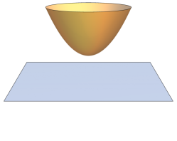
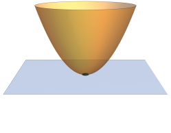
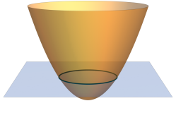
Figure 1: The energy dispersion for (a) insulator, (b) critical point and (c) metal plotted in the two-dimensional momentum space. The dot in (b) represents the bottom of the band which touches the chemical potential at the critical point, and the circle in (c) represents the Fermi surface.

To set up the RG procedure, we divide $\mathcal{S}$ into a reference action and a deformation. The reference action is chosen to be the ultra-local theory which describes the insulating fixed point,

$$\mathcal{S}_{0}=m\sum_{i}(\bar{\bm{\psi}}_{i}\cdot{\bm{\psi}}_{i}),$$ (3)

and the rest is treated as a deformation,

$$\mathcal{S}_{1}=-\sum_{ij}t^{(0)}_{ij}(\bar{\bm{\psi}}_{i}\cdot{\bm{\psi}}_{j})+\frac{\lambda}{N}\sum_{i}(\bar{\bm{\psi}}_{i}\cdot{\bm{\psi}}_{i})^{2}.$$ (4)

Following Lee2016 , we define quantum states associated with $S_{0}$ and $S_{1}$ as

$$|S_{0}\rangle = \int D\bar{\psi}D\psi~{}e^{-S_{0}[\bar{\psi},\psi]}|\bar{\psi},\psi\rangle,$$

$$|S_{1}\rangle = \int D\bar{\psi}D\psi~{}e^{-S_{1}[\bar{\psi},\psi]}|\bar{\psi},\psi\rangle,$$ (5)

where $|\bar{\psi},\psi\rangle$ are the basis states labeled by the Grassmannian fields,

$$|\bar{\psi},\psi\rangle=\prod_{i,a}(1-\bar{\psi}_{i}^{a}c_{1i}^{a\dagger})(1-\psi_{i}^{a}c_{2i}^{a\dagger})|0\rangle.$$ (6)

The basis states are constructed from a Fock space which can accommodate up to $2N$ auxiliary fermions at each site on the $D$-dimensional spacetime lattice : $c_{1i}^{a\dagger}$ ($c_{2i}^{a\dagger}$) with $a=1,2,..,N$ represents the creation operator of the fermions associated with $\bar{\psi}_{i}^{a}$ ($\psi_{i}^{a}$), and $|0\rangle$ is the vacuum annihilated by $c_{\alpha i}^{a}$. It is emphasized that the auxiliary fermions occupy sites in the $D$-dimensional spacetime lattice, and they are different from the original fermions that live on the $(D-1)$-dimensional space. We define an inner product between quantum states defined in spacetime as

$$\langle\Psi^{\prime}||\Psi\rangle\equiv\langle\Psi^{\prime}|O|\Psi\rangle$$ (7)

with $O\equiv\prod_{i,a}(c_{1i}^{a\dagger}-c_{1i}^{a})(c_{2i}^{a\dagger}-c_{2i}^{a})$. The inner product is chosen such that the basis states satisfy the orthonormality condition,

$$\langle\psi^{\prime},\bar{\psi}^{\prime}||\bar{\psi},\psi\rangle=\prod_{i,a}\delta(\bar{\psi}_{i}^{{}^{\prime}a}-\bar{\psi}_{i}^{a})\delta(\psi_{i}^{{}^{\prime}a}-\psi_{i}^{a}),$$ (8)

where $\langle\psi^{\prime},\bar{\psi}^{\prime}|$ is the Hermitian conjugate of $|\psi^{\prime},\bar{\psi}^{\prime}\rangle$. Then the partition function is given by the overlap between the two quantum states,

$$Z=\int D\bar{\psi}D\psi~{}e^{-S_{0}[\bar{\psi},\psi]-S_{1}[\bar{\psi},\psi]}=\langle S_{0}^{\prime}||S_{1}\rangle,$$ (9)

where $|S_{0}^{\prime}\rangle$ is the complex conjugate of $|S_{0}\rangle$.

Renormalization group flow can be understood as a quantum evolution of $|S_{1}\rangle$ generated by an operator $\hat{H}$Lee2016 . Since the partition function is invariant under the coarse-graining transformation,

$$Z=\langle S_{0}^{\prime}||S_{1}\rangle=\langle S_{0}^{\prime}||e^{-dz\hat{H}}|S_{1}\rangle,$$ (10)

where $dz$ is an infinitesimal parameter, the reference state should be annihilated by $\hat{H}$,

$$\hat{H}^{\dagger}O^{\dagger}|S_{0}^{\prime}\rangle=0.$$ (11)

This is equivalent to the statement that $S_{0}$ represents a fixed point. Because $|S_{0}^{\prime}\rangle$ is a direct-product state in spacetime, the coarse graining operator that satisfies Eq. (11) is ultra-local,

$$\hat{H}=\sum_{i,a}\left[-\frac{2}{m}c_{1i}^{a\dagger}c_{2i}^{a\dagger}+c_{1i}^{a}c_{1i}^{a\dagger}+c_{2i}^{a}c_{2i}^{a\dagger}\right].$$ (12)

The evolution generated by $\hat{H}$ corresponds to a real space coarse graining in which the mass $m$ is gradually increased such that fluctuations of fields are suppressed at each siteLunts2015 . While $\hat{H}$ is not Hermitian, it can be mapped to a Hermitian operator through a similarity transformation as all eigenvalues are real. As the evolution operators are repeatedly inserted between the overlap, $e^{-z\hat{H}}|S_{1}\rangle$ is gradually projected to the unentangled ground state of $\hat{H}$. Whether the initial state $|S_{1}\rangle$ can be smoothly projected to the direct product state depends on whether the system belongs to the insulating phase described by the reference actionLee2016 .

Now we fix $\lambda$, and label the state associated with the deformation in terms of hopping amplitudes,

$$|t\rangle=\int D\bar{\psi}D\psi~{}e^{\sum_{i,j}t_{ij}\bar{\psi}_{i}\cdot\psi_{j}-\frac{\lambda}{N}\sum_{i}(\bar{\psi}_{i}\cdot\psi_{i})^{2}}|\bar{\psi},\psi\rangle.$$ (13)

Apart from the fixed quartic interaction, $|t\rangle$ contains only single-trace hoppings. However, multi-trace operators are generated under the coarse graining evolution. In quantum RG, the multi-trace operators are traded with non-trivial dynamics of the single-trace sourcesLee2012 ; Lee:2012xba ; Lee:2013dln . As a result, the partition function is given by a path integration over the scale dependent single-trace sources $t_{ij}(z)$Lunts2015 ; Lee2016 ,

$$Z = \lim_{z\rightarrow\infty}\langle S_{0}^{{}^{\prime}}||e^{-{z}\hat{H}}|t^{(0)}\rangle=\left.\int Dt(z)Dt^{*}(z)~{}~{}\langle S_{0}^{{}^{\prime}}||t(\infty)\rangle~{}e^{-N\int_{0}^{\infty}dz\left(t^{*}_{ij}\partial_{z}t_{ij}+{\cal H}[t^{*},t]\right)}\right|_{t_{ij}(0)=t^{(0)}_{ij}},$$

where ${\cal H}[t^{*},t]$ is the coherent state representation of the bulk Hamiltonian $\hat{\mathcal{H}}$ given by

$$\hat{\mathcal{H}} = \sum_{i}\Big{[}\frac{2}{m}t_{ii}+\frac{4\lambda(-1+\frac{1}{N})}{m}t_{ii}^{\dagger}-4\lambda(t_{ii}^{\dagger})^{2}-\frac{8\lambda^{2}}{m}(t_{ii}^{\dagger})^{3}\Big{]}$$ (15)

$$+\sum_{i,j}\Big{[}2+\frac{4\lambda}{m}(t_{ii}^{\dagger}+t_{jj}^{\dagger})\Big{]}t_{ij}^{\dagger}t_{ij}-\frac{2}{m}\sum_{i,j,k}\Big{[}t_{kj}^{\dagger}t_{ki}t_{ij}\Big{]}.$$

Here the gauge is fixed so that the speed of coarse graining is uniform in spacetime, and the shift is zero at all $z$Lee2016 . The bi-local fields are the fundamental degrees of freedom in the bulk, which include the metric and higher spin fields. In the Hamiltonian picture, the bi-local fields are promoted to quantum operators : $t_{ij}$ ($t_{ij}^{\dagger}$) represents the annihilation (creation) operator of quantized link between sites $i$ and $j$. Despite the fact that the original theory is fermionic, the bulk theory is bosonic because there is no U(N) invariant fermionic operator in the theory.

In the large $N$ limit, quantum fluctuations in the RG path are suppressed, and the saddle point approximation becomes reliable. The saddle point equation reads

$$\begin{aligned} \partial_{z}\bar{t}_{ij}&=-2\Big{\{}-\frac{2\lambda\delta_{ij}}{m}-\delta_{ij}[4\lambda+\frac{12\lambda^{2}}{m}\bar{p}_{ii}]\bar{p}_{ii}+\frac{2\lambda\delta_{ij}}{m}\sum_{k}(\bar{t}_{ik}\bar{p}_{ik}+\bar{t}_{ki}\bar{p}_{ki})\\ &+[1+\frac{2\lambda}{m}(\bar{p}_{ii}+\bar{p}_{jj})]\bar{t}_{ij}-\frac{1}{m}\sum_{k}\bar{t}_{ik}\bar{t}_{kj}\Big{\}},\\ \partial_{z}\bar{p}_{ij}&=2\Big{\{}\frac{\delta_{ij}}{m}+[1+\frac{2\lambda}{m}(\bar{p}_{ii}+\bar{p}_{jj})]\bar{p}_{ij}-\frac{1}{m}\sum_{k}(\bar{p}_{ik}\bar{t}_{jk}+\bar{t}_{ki}\bar{p}_{kj})\Big{\}}.\end{aligned}$$ (16)

Here $\bar{t}_{ij}(z)$ and $\bar{p}_{ij}(z)$ denote the saddle point configuration of $t_{ij}(z)$ and $t_{ij}^{*}(z)$, which satisfy the boundary conditions,

$$\bar{t}_{ij}(0)=t_{ij}^{(0)},$$ (17)

$$\bar{p}_{ij}(\infty)=\frac{1}{N}\left.\frac{\partial ln\langle S_{0}^{{}^{\prime}}||\bar{t}\rangle}{\partial\bar{t}_{ij}}\right|_{z=\infty}.$$ (18)

It is noted that $\bar{p}_{ij}$ is not necessarily the complex conjugate of $\bar{t}_{ij}$ at the saddle point. If $t_{ij}^{(0)}$ depends only on $r_{i}-r_{j}$, the saddle point solution is also invariant under the translation. In this case, the equations in momentum space are reduced to

$$\partial_{z}\bar{T}_{q} = -2\Bigg{\{}-\frac{2\lambda}{m}-\left[4\lambda+\frac{12\lambda^{2}}{m}\bar{p}_{0}\right]\bar{p}_{0}+\frac{4\lambda}{Vm}\sum_{q^{{}^{\prime}}}\bar{T}_{q^{{}^{\prime}}}\bar{P}_{q^{{}^{\prime}}}+\left[1+\frac{4\lambda}{m}\bar{p}_{0}\right]\bar{T}_{q}-\frac{1}{m}(\bar{T}_{q})^{2}\Bigg{\}},$$ (19)

$$\partial_{z}\bar{P}_{q} = \frac{2}{m}+2\left[1+\frac{4\lambda}{m}\bar{p}_{0}\right]\bar{P}_{q}-\frac{4}{m}\bar{P}_{q}\bar{T}_{q},$$ (20)

where $\bar{T}_{q}=\sum_{r}\bar{t}_{i+r,i}e^{iqr}$, $\bar{P}_{q}=\sum_{r}\bar{p}_{i+r,i}e^{-iqr}$, $\bar{p}_{0}\equiv\bar{p}_{ii}=\frac{1}{V}\sum_{q}\bar{P}_{q}$. $q=(\omega,k)$ denotes frequency, $\omega$ and $(D-1)$-dimensional momentum, $k=(k_{1},k_{2},..,k_{D-1})$. The solution to the saddle point equations is given by

$$\bar{P}_{q}(z)=-\frac{e^{-2z}}{-i\bar{T}_{q}(0)+m+2\lambda p_{0}(0)}-(1-e^{-2z})\frac{1}{m},$$ (21)

$$\bar{T}_{q}(z)=-\frac{2\lambda}{m}+m+\frac{2\lambda}{m}e^{-2z}(m\bar{p}_{0}(0)+1)+\frac{1}{\bar{P}_{q}(z)}.$$ (22)

Eqs. (21) and (22) completely determine the saddle-point configurations of the bulk fields in terms of $\bar{T}_{q}(0)$, which encodes all the information about the microscopic theory. For example, the $(D-1)$-dimensional hypercubic lattice with a continuous imaginary time gives $\bar{T}_{q}(0)=-i\omega-2t\sum_{i=1}^{D-1}\cos(k_{i})-\mu$, where $t$ is the nearest neighbor hopping amplitude and $\mu$ is the chemical potential. In general, any local hopping in space can be written in power series of $k$,

$$\bar{T}_{q}(0)=\bar{T}_{0}(0)-i\omega-e(k),$$ (23)

where

$$e(k)=\bm{k}^{2}+\sum_{n=2}^{\infty}\frac{c_{i_{1},i_{2},..,i_{2n}}}{m^{n-1}}k_{i_{1}}k_{i_{2}}..k_{i_{2n}}.$$ (24)

Here the chemical potential $\bar{T}_{0}(0)$ is singled out, and the coefficient of the quadratic term is normalized by rescaling $k$. $c_{i_{1},i_{2},..,i_{2n}}$ can be independently tuned by further neighbor hoppings on a microscopic lattice. It is assumed that the minimum of the band is $k=0$, and the lattice respects the parity to allow only even powers of momentum in the dispersion. In terms of $e(k)$, the saddle point solutions are written as

$$\bar{P}_{q}(z) = -\frac{e^{-2z}}{i\omega+e(k)+\delta}-(1-e^{-2z})\frac{1}{m},$$

$$\bar{T}_{q}(z) = -\frac{2\lambda}{m}+m+\frac{2\lambda}{m}e^{-2z}(m\bar{p}_{0}(0)+1)-m\frac{i\omega+e(k)+\delta}{(1-e^{-2z})(i\omega+e(k)+\delta)+me^{-2z}},$$ (25)

where $\delta=-\bar{T}_{0}(0)+m+2\lambda\bar{p}_{0}(0)$ is the gap.

III Emergent geometry in the bulk

Because the reference state is ultra-local, there is no background metric in the bulk. The bulk geometry is dynamically determined by the saddle point solution. Since the bulk theory involves the bi-local fields of all sizes, it is kinematically non-local. A sense of locality emerges only when single-trace sources decay fast enough in spacetime. In this section, we examine the geometry that emerges in the bulk in the insulating phase and in the metallic phase.

III.1 Insulating phase

To study the behavior of the hopping field in real space, we first transform $\bar{T}_{q}(z)$ to the time domain,

$$\bar{T}_{\tau,\bm{k}}(z)=\int\bar{T}_{\omega,k}(z)e^{-i\omega\tau}\frac{d\omega}{2\pi}=\frac{m^{2}e^{2z}}{(e^{2z}-1)^{2}}\Bigl{[}-\theta(\tau)\theta(-E(\bm{k},z))+\theta(-\tau)\theta(E(\bm{k},z))\Bigr{]}e^{E(\bm{k},z)\tau},$$ (26)

where

$$E(\bm{k},z)=e(k)+\delta+\frac{m}{e^{2z}-1}.$$ (27)

$\theta(\tau)$ is the theta function, and ultra-local terms are ignored. In the insulating phase with $\delta>0$, $E(\bm{k},z)$ is positive for all $k$ and $z$, and the first term on the right hand side of Eq. (26) vanishes. Because $E(\bm{k},z)$ is analytic in $k$, the hopping field decays exponentially in real space at all $z$. For example, for $e(k)=k^{2}$ the bi-local field in the real space is given by

$$\bar{t}_{i+r,i}(z)=\int\bar{T}_{\tau,\bm{k}}(z)e^{-i\bm{k}\cdot\bm{x}}\frac{d\bm{k}}{(2\pi)^{d-1}}=\left(\frac{1}{2\sqrt{-\pi\tau}}\right)^{d-1}\frac{m^{2}e^{2z}}{(e^{2z}-1)^{2}}\theta(-\tau)e^{(\delta+\frac{m}{e^{2z}-1})\tau}e^{\frac{\bm{x}^{2}}{4\tau}},$$ (28)

where $r=(\tau,x)$ with $x=(x_{1},x_{2},..,x_{D-1})$ representing $(D-1)$-dimensional vector in real space.

Fluctuations of the bi-local fields propagate on the background set by the saddle-point configuration. Therefore, the bulk geometry can be extracted by inspecting the equation of motions obeyed by the fluctuations of the hopping fields around the saddle point,

$$\tilde{t}_{ij} =t_{ij}-\bar{t}_{ij},$$ (29)

$$\tilde{p}_{ij} =t_{ij}^{*}-\bar{p}_{ij}.$$

The quadratic action for the fluctuations is

$$S_{2} =\int dz\Bigg{\{}-4\lambda\sum_{i}\left(1+\frac{6\lambda}{m}\bar{p}_{0}\right)\tilde{p}_{ii}^{2}$$ (30)

$$+\sum_{ij}\left[\tilde{p}_{ij}\left(\partial_{z}+2+\frac{8\lambda}{m}\bar{p}_{0}\right)\tilde{t}_{ij}+\frac{4\lambda}{m}(\tilde{p}_{ii}+\tilde{p}_{jj})\left(\bar{p}_{ij}\tilde{t}_{ij}+\bar{t}_{ij}\tilde{p}_{ij}\right)\right]$$

$$-\frac{2}{m}\sum_{ijk}\left(\bar{p}_{ij}\tilde{t}_{ik}\tilde{t}_{kj}+\bar{t}_{ik}\tilde{p}_{ij}\tilde{t}_{kj}+\bar{t}_{kj}\tilde{p}_{ij}\tilde{t}_{ik}\right)\Bigg{\}}.$$

To extract the background metric, we focus on the imaginary part of the hopping field $\tilde{t}_{ij}^{A}=\tilde{t}_{ij}-\tilde{t}_{ij}^{*}$ which satisfies a simple equation of motion,

$$\left(\partial_{z}+2+\frac{8\lambda}{m}\bar{p}_{0}(z)\right)\tilde{t}^{A}_{ij}-\frac{2}{m}\left(\bar{t}_{ik}\tilde{t}^{A}_{kj}+\bar{t}_{kj}\tilde{t}^{A}_{ik}\right)=0$$ (31)

for $i\neq j$. We take the continuum limit, and define $\tilde{t}_{ij}^{A}=e^{-2z}\tilde{t}^{A}(r,r^{\prime},z)$, where $r$ and $r^{\prime}$ represent spacetime coordinates $(\tau,\bm{x})$ and $(\tau^{\prime},\bm{x}^{\prime})$. For large $z$ and $r\neq r^{\prime}$, the equation of motion becomes

$$\left[(m+\delta e^{2z})\partial_{z}+4\delta-\frac{2m}{1-\frac{\partial_{\tau}+e(\partial_{i})}{me^{-2z}+\delta}}-\frac{2m}{1-\frac{-\partial_{\tau}^{\prime}+e(\partial_{i}^{{}^{\prime}})}{me^{-2z}+\delta}}\right]\tilde{t}^{A}(r,r^{\prime},z)=0,$$ (32)

where $\partial_{i}\equiv\frac{\partial}{\partial x_{i}}$, $\partial_{i}^{{}^{\prime}}\equiv\frac{\partial}{\partial x_{i}^{{}^{\prime}}}$. This can be written in a covariant form,

$$\Bigg{[}\sqrt{g^{zz}(z)}\partial_{z}+4\delta-\frac{2m}{1-\frac{1}{m}\left(\sqrt{g^{\tau\tau}(z)}\partial_{\tau}+g^{ij}(z)\partial_{i}\partial_{j}+\sum_{n>1}\frac{\tilde{c}_{i_{1},..,i_{2n}}(z)}{m^{n-1}}\partial_{i_{1}}..\partial_{i_{2n}}\right)}$$

$$-\frac{2m}{1-\frac{1}{m}\left(-\sqrt{g^{\tau\tau}(z)}\partial_{\tau^{\prime}}+g^{ij}(z)\partial_{i}^{\prime}\partial_{j}^{\prime}+\sum_{n>1}\frac{\tilde{c}_{i_{1},..,i_{2n}}(z)}{m^{n-1}}\partial_{i_{1}}^{\prime}..\partial_{i_{2n}}^{\prime}\right)}\Bigg{]}\tilde{t}^{A}(r,r^{\prime},z)=0,$$ (33)

where $\sqrt{g^{zz}}(z)=m+\delta e^{2z}$, $\sqrt{g^{\tau\tau}}(z)=g^{ii}(z)=\frac{m}{me^{-2z}+\delta}$, $\tilde{c}_{i_{1},..,i_{2n}}(z)=\frac{m}{me^{-2z}+\delta}c_{i_{1},..,i_{2n}}$. The bulk metric is identified from the terms up to two derivatives,

$$ds^{2}=\frac{dz^{2}}{(m+\delta e^{2z})^{2}}+(e^{-2z}+\delta/m)^{2}d\tau^{2}+(e^{-2z}+\delta/m)d\bm{x}^{2}.$$ (34)

$\tilde{c}_{i_{1},..,i_{2n}}(z)$ encodes the vacuum expectation values of the higher spin fields in the bulk.

In the insulating phase, the geometry ends at a finite proper distance from the UV boundary,

$$L=\int_{0}^{\infty}\frac{dz}{m+\delta e^{2z}}=\frac{log(\frac{m+\delta}{\delta})}{2m}.$$ (35)

The finite depth in the bulk reflects the fact that the quantum state associated with the action can be smoothly projected to the direct product state through a series of RG transformations with a finite depth. The proper distance in the radial direction measures the “distance” between theoriesLee2016 .

III.2 Metallic phase

As the system deviates further from the insulating state with decreasing gap, the depth of the bulk space diverges logarithmically. When the system reaches the critical point at $\delta=0$, the bulk geometry develops an infinitely long throat with a Lifhistz horizon at $z=\infty$. At the critical point, the metric in Eq. (34) becomes the Lifshitz geometry,

$$ds^{2}=\frac{dz^{2}}{m^{2}}+e^{-4z}d\tau^{2}+e^{-2z}d\bm{x}^{2}$$ (36)

which is invariant under the scaling

$$z\to z+s,~{}\tau\to e^{2s}\tau,~{}\bm{x}\to e^{s}\bm{x}.$$ (37)

The dynamical critical exponent $z=2$ reflects the quadratic dispersion at the bottom of the band in Eq. (23). The isometry of the bulk metric is expected from the form of the hopping field in Eq. (28) which is invariant under Eq. (37) at $\delta=0$. If one tuned parameters in $t_{ij}$ at UV to make the dispersion to scale as $\bar{T}_{q}(0)\sim k^{2r}$ at the bottom of the band, the resulting geometry would have the dynamical critical exponent $2r$. It is noted that the higher-derivative terms in Eq. (33) are suppressed by the curvature scale in the bulk. For the locality at a shorter length scale in the bulk, there are stringent constraints on field theoriesHeemskerk:2009pn ; Nakayama2015 ; 2016arXiv161105315S .

At the critical point, the Lifshitz horizon is located at $z=\infty$. However, the horizon arises at a finite $z$ in the metallic phase. Unlike the bosonic modelLee2016 , the chemical potential can be further increased across the bottom of the band. For $\delta<0$, a Fermi surface forms, and the system becomes a metal. In the metallic phase, the horizon moves to $z_{H}\equiv\frac{1}{2}log(1+\frac{m}{-\delta})$ at which $g_{\tau\tau}$ vanishes. Outside the horizon, $E(\bm{k},z)$ remains positive for all $k$, and the metric is given by

$$ds^{2}=\frac{dz^{2}}{4m^{2}(z_{H}-z)^{2}}+\frac{4\delta^{2}}{m^{2}}(z_{H}-z)^{2}d\tau^{2}+\frac{-2\delta}{m}(z_{H}-z)d\bm{x}^{2}$$ (38)

for small $z_{H}-z$ with $z_{H}>>1$. The geometry no longer has an isometry associated with a global translation of $z$ because there is a scale represented by $z_{H}$. However, the space outside the horizon has an isometry associated with rescaling of $z$ toward $z_{H}$. The isometry becomes manifest in a new coordinate system, $z^{\prime}=-\frac{1}{2}log(z_{H}-z)$, $\tau^{\prime}=-\frac{2\delta}{m}\tau$, $\bm{x}^{\prime}=\sqrt{\frac{-2\delta}{m}}\bm{x}$ in which the metric reduces to the Lifshitz geometry in Eq. (36). Although the horizon arises at a finite $z$, the proper distance from the UV boundary to the horizon is still infinite. This is consistent with the fact that the metallic state belongs to a different universality class from the insulating state.

Although the metric near the horizon takes the universal form, the background higher-spin fields, $\tilde{c}_{i_{1},..,i_{2n}}(z)$ encodes the information about the microscopic details such as the underlying lattice and further neighbor hoppings in the boundary theoryPROP:PROP200410203 ; Grumiller2016 ; PhysRevLett.116.231301 . The effect of the higher-spin hair on the fluctuation fields in Eq. (33) depends on the momentum of the fluctuation mode and the radial position. For a mode whose proper momentum is $O(\sqrt{m})$ at radial location $z$, the $2n$ derivative term in Eq. (33) scales as $(z_{H}-z)^{(n-1)}$. The bulk equation of motion for the low-momentum modes becomes insensitive to the higher-spin fields close to the horizon. However, in order to extract the full low-energy data from the UV boundary, one should probe particle-hole excitations whose momenta are comparable to the Fermi momentum $k_{F}\sim\sqrt{|\delta|}$. If a mode with proper momentum $k_{F}$ at the UV boundary is sent into the bulk, the momentum is blue shifted to $p\sim\sqrt{\frac{|\delta|}{(z_{H}-z)}}$ near the horizon. For these modes, the higher-derivative terms in Eq. (33) remain important. The sensitivity to the higher-spin fields signifies the need to go beyond the low-energy effective theory near the horizon. This is expected because the shape of Fermi surface is determined not just by the quadratic term but also by all higher-order terms in Eq. (24).

The horizon corresponds to a phase transition at which the length scale associated with the size of bi-local operators in $e^{-z\hat{H}}|S_{1}\rangle$ divergesLee2016 . At the horizon, the range of hoping diverges, which causes the collapse of the $D$-dimensional spacetime volume. Zero area of the horizon is consistent with the fact that the metal has zero entropy density. Although the Lifshitz horizon has a divergent tidal force, nothing stops one from being able to continue the coarse graining procedure across the horizon. Inside the horizon with $z>z_{H}$, $E(\bm{k},z)$ changes sign as a function of momentum. The discontinuity of $\bar{T}_{\tau,\bm{k}}(z)$ as a function of momentum results in a slow decay of the hopping field along with a Friedel-like oscillation in real space. The specific form of the oscillation depends on the microscopic details. From now on, we will focus on the dispersion $e(k)=k^{2}$, which describes the spherical Fermi surface. For different shapes of Fermi surface, the structure inside the horizon will be different. For the spherical Fermi surface, $E(\bm{k},z)$ becomes negative for $|k|<k_{s}(z)\equiv\sqrt{-\delta-\frac{m}{e^{2z}-1}}$,

$$\bar{T}_{\tau,\bm{k}}(z)=\frac{m^{2}e^{2z}}{(e^{2z}-1)^{2}}\Big{(}-\theta(\tau)\theta(k_{s}(z)-|\bm{k}|)+\theta(-\tau)\theta(|\bm{k}|-k_{s}(z))\Big{)}e^{(\bm{k}^{2}-k_{s}(z)^{2})\tau}.$$ (39)

The asymptotic behavior of $\bar{t}_{i+r,i}$ as a function of $r=(\tau,x)$ is given by $t_{i+r,i}=\frac{m^{2}e^{2z}}{(e^{2z}-1)^{2}}K(\tau,x;z)$, where

$$K(\tau,x;z)\sim-\frac{\cos(k_{s}(z)x)}{2\pi k_{s}(z)\tau}+O(\frac{1}{\tau^{2}}),\textrm{ as }|\tau|\to\infty,$$ (40)

$$K(\tau,x;z)\sim-\frac{\sin(k_{s}(z)x)}{\pi x}+O(\frac{1}{x^{2}}),\textrm{ as }x\to\infty$$ (41)

in $D=1+1$, and

$$K(\tau,x;z)\sim-\frac{1}{8\pi^{2}\tau}\cdot J_{0}(k_{s}(z)|x|)+O(\frac{1}{\tau^{2}}),\textrm{ as }|\tau|\to\infty,$$ (42)

$$K(\tau,x;z)\sim-\sqrt{\frac{k_{s}(z)}{2\pi^{3}|\bm{x}|^{3}}}\cdot\sin(k_{s}(z)|\bm{x}|-\frac{\pi}{4})+O(|\bm{x}|^{-\frac{5}{2}}),\textrm{ as }\bm{x}\to\infty$$ (43)

in $D=2+1$, where $J_{0}(x)$ is the 0th order Bessel function of the first kind.

Inside the horizon, the saddle point configuration of the hopping field decays in a power-law as a function of $r$. The hopping field sets a non-local background on which fluctuation fields propagate according to Eq. (31). In the large $z$ limit, the equation of motion for $\tilde{t}^{A}(\tau,x,\tau^{\prime},x^{\prime},z)$ becomes

$$(me^{2z}~{}\partial_{z}+4m)\tilde{t}^{A}(\tau,x,\tau^{\prime},x^{\prime},z)-2m^{2}\int d\tau_{1}dx_{1}~{}K(\tau-\tau_{1},x-x_{1};z)~{}\tilde{t}^{A}(\tau_{1},x_{1},\tau^{\prime},x^{\prime},z)$$

$$~{}~{}~{}~{}~{}~{}-2m^{2}\int d\tau^{\prime}_{1}dx^{\prime}_{1}~{}\tilde{t}^{A}(\tau,x,\tau^{\prime}_{1},x^{\prime}_{1},z)~{}K(\tau^{\prime}_{1}-\tau^{\prime},x^{\prime}_{1}-x^{\prime};z)=0,$$ (44)

where the asymptotic behavior of $K(\tau,x;z)$ is given in Eqs.(40)-(43). The non-local saddle point configuration allows the bi-local fields to jump to far sites in the $D$-dimensional spacetime. This implies that the space inside the horizon can not be described by a local geometry.

The wavevector for the Friedel-like oscillation at radial position $z$ is given by $k_{s}(z)$, which gradually increases from $0$ at $z_{H}$ to the true Fermi momentum $k_{F}=\sqrt{-\delta}$ in the large $z$ limit. $k_{s}(z)$ can be regarded as the size of the Fermi surface with a $z$-dependent chemical potential $\mu(z)=-\delta-\frac{m}{e^{2z}-1}$. As $z$ increases from the horizon, the bulk effectively scans through the occupied states from the bottom of the band to the Fermi level. Therefore, the non-local structure inside the horizon is determined by the full dispersion below the Fermi surface. The region deep inside the horizon keeps the data on the low-energy modes close to the Fermi surface. Different metals have different non-local structures in the large $z$ limit because the Fermi liquids have infinitely many marginal deformations, including the shape of the Fermi surface. On the other hand, the region close to the horizon in the interior is sensitive to the occupied states below the Fermi surface, which is not part of the universal low-energy data of the boundary theory. A change in the shape of the band below the Fermi surface that does not involve a change near the Fermi surface does affect the wavevector of the oscillation near the horizon. This implies that the interior of the horizon keeps not only the universal low-energy data of the theory but also non-universal microscopic information of the boundary field theory.

IV Summary and Discussion

In this paper, we apply the quantum renormalization group to construct the holographic dual of the fermionic $U(N)$ vector model with a nonzero charge density. The bulk equations of motion are exactly solved in the large $N$ limit to derive the geometries that emerge in different phases of the model. In the insulating phase, the bulk geometry caps off at a finite proper distance in the radial direction. At the critical point between the metal to insulator phase transition, the proper size in the radial direction diverges, which results in a Lifshitz geometry in the bulk. In the metallic phase, the Lifshitz horizon moves to a finite radial coordinate. The geometry outside of the Lifshitz horizon carries a higher-spin hair determined by microscopic hopping amplitudes of the boundary theory. On the other hand, the interior of the horizon is characterized by an algebraic non-locality, and can not be described by a Riemannian geometry. Certain microscopic data of the boundary field theory is encoded in the interior of the horizon.

The non-local space inside the horizon is different from a globally connected network where every site is connected to every other sites with an equal hopping strength. Since the non-local connectivity decreases as a power-law in coordinate distance, there is still a sense in which certain points are ‘closer’ than other points to a given point. However, this notion of distance can not be captured within the framework of Riemannian geometry. In order to define a notion of distance in this space, one might rewrite the non-local kernel in Eq. (44) as

$$K(\tau,x)=\tilde{K}(\tau,x)e^{-md(\tau-\tau_{1},x-x_{1})},$$ (45)

where $\tilde{K}(\tau,x)$ is a function which captures the modulation in the sign of the hopping function with $|\tilde{K}(\tau,x)|\sim 1$ and $d(\tau,x)$ is a function that measures physical distance. The idea behind this is to define the physical distance by insisting that the kernel in the kinetic term decays exponentially. This agrees with the geodesic distance measured by the metric in Eq. (38) outside the horizon, but the definition is general enough to be applicable to the region inside the horizon. Because the hopping amplitude decays in power-law in Eq. (41) and Eq. (43), the distance between two points increases only logarithmically in coordinate, e.g. $d(x,y)\sim\frac{1}{m}\log|x-y|$. No metric on a Riemannian manifold can reproduce the distance function of this form. One way of obtaining such distance function is by embedding the space in a higher dimensional Riemannian space, and define the distance between two points on the original space in terms of geodesics that can go through the higher dimensional space. For example, the logarithmic distance function can be obtained from the geodesic distance between points on the boundary of a hyperbolic space (see Fig. 2). The non-local geometry is ‘anomalous’ in that distance function can be realized from a local metric only through a higher-dimensional space.

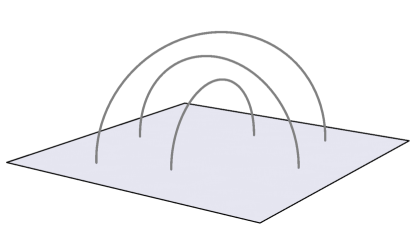
Figure 2: Examples of geodesics in the three-dimensional hyperbolic space ${\bf H}_{3}$. The shortest geodesic distances between two points on the plane scales logarithmically in the coordinate distance in the plane.

For $D>2$, the metallic state becomes unstable against superconductivity at an energy scale which is exponentially small in $N$. As a result, the geometry for the metallic state becomes unstable once quantum fluctuations are included in the bulk. However, this should not be the case for all metals. If one breaks the parity and the time-reversal symmetry, one can have a Fermi liquid state without perturbative superconducting instability. The geometries dual to those stable metals are expected to exhibit similar non-local structures behind the horizon.

Since we use the imaginary time formalism in this study, the bulk theory captures only the ground state of the theory. It shows how bulk geometry depends on the microscopic information of the ground state determined by Hamiltonian. It will be interesting to extend this to the real time formalism to understand the dependence of bulk geometry on state and Hamiltonian separately.

Appendix A Asymptotic Behavior of $\bar{T}_{\tau,x}$

In this appendix, we examine the asymptotic behavior of $\bar{t}_{i+r,i}$ as $|\tau|\to\infty$ and $x\to\infty$ in $D=1+1$ and $D=2+1$. In $1+1$ dimensions, the Fourier transform of Eq. (39) gives

$$\bar{t}_{i+r,i}(z)=\frac{m^{2}e^{2z}}{(e^{2z}-1)^{2}}\cdot e^{-k_{s}^{2}\tau}\cdot\frac{e^{\frac{x^{2}}{4\tau}}}{4\sqrt{\pi}}\Big{[}-\theta(\tau)\frac{i}{\sqrt{\tau}}\Big{(}erf(\frac{x-2ik_{s}\tau}{2\sqrt{\tau}})-erf(\frac{x+2ik_{s}\tau}{2\sqrt{\tau}})\Big{)}$$ (46)

$$+\theta(-\tau)\frac{1}{\sqrt{-\tau}}\Big{(}2-erf(\frac{ix-2k_{s}\tau}{2\sqrt{-\tau}})+erf(\frac{ix+2k_{s}\tau}{2\sqrt{-\tau}})\Big{)}\Big{]},$$

where $erf(x)$ is the error function. The asymptotic form is given by Eq. (40) and Eq. (41).

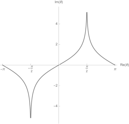
Figure 3: integral contour of $\theta$ where Re$(\cos\theta)=\pm 1$

In $2+1$ dimensions, the Fourier transformation of Eq. (39) becomes

$$\bar{t}_{i+r,i}(z)= \int_{-\pi}^{\pi}\int_{0}^{\infty}\bar{T}_{\tau,\bm{k}}(z)e^{-ikxcos\theta}\cdot k\cdot\frac{dkd\theta}{(2\pi)^{2}}.$$ (47)

For large $|\tau|$, Eq. (39) shows that $\bar{T}_{\tau,k}(z)$ falls very fast as $|k|$ goes away from $k_{s}$. Since the integration over $k$ is concentrated near $k_{s}$, we obtain

$$\int_{0}^{\infty}\bar{T}_{\tau,\bm{k}}(z)e^{-ikxcos\theta}\cdot k\cdot\frac{dk}{2\pi} =-\frac{m^{2}e^{2z}}{(e^{2z}-1)^{2}}\int_{0}^{k_{s}}e^{(k^{2}-k_{s}^{2})\tau}e^{-ikxcos\theta}\cdot k\cdot\frac{dk}{2\pi}$$ (48)

$$\approx-\frac{m^{2}e^{2z}}{(e^{2z}-1)^{2}}\int_{-\infty}^{k_{s}}k_{s}\cdot e^{2k_{s}(k-k_{s})\tau}e^{-ik_{s}xcos\theta}\frac{dk}{2\pi}$$

$$=-\frac{m^{2}e^{2z}}{(e^{2z}-1)^{2}}\cdot\frac{1}{4\pi\tau}\cdot e^{-ik_{s}xcos\theta},$$

and

$$\bar{t}_{i+r,i}\approx -\frac{m^{2}e^{2z}}{(e^{2z}-1)^{2}}\cdot\frac{1}{8\pi^{2}\tau}\int_{-\pi}^{\pi}e^{-ik_{s}xcos\theta}d\theta$$ (49)

$$= -\frac{m^{2}e^{2z}}{(e^{2z}-1)^{2}}\cdot\frac{1}{8\pi^{2}\tau}\cdot J_{0}(k_{s}x).$$

On the other hand, for large $|x|$, we first perform the radial integration in momentum to obtain

$$\int_{0}^{\infty}\bar{T}_{\tau,\bm{k}}(z)e^{-ikxcos\theta}\cdot k\cdot\frac{dk}{2\pi}\approx\frac{m^{2}e^{2z}}{(e^{2z}-1)^{2}}\cdot\frac{k_{s}e^{-ik_{s}xcos\theta}}{2i\pi xcos\theta}.$$ (50)

To evaluate the remaining angle integration,

$$\bar{t}_{i+r,i}\approx \frac{m^{2}e^{2z}}{(e^{2z}-1)^{2}}\cdot\frac{k_{s}}{4i\pi^{2}}\int_{-\pi}^{\pi}\frac{e^{-ik_{s}xcos\theta}}{xcos\theta}d\theta$$ (51)

we use the method of steepest descent for large $|x|$, where the integral contour is deformed as in Fig. 3. The main contributions are from $\theta=\pm\pi$ and $\theta=0$. Expansions around these points give Eq. (43).

References

- (1) S. W. Hawking, Particle creation by black holes, Communications in Mathematical Physics 43 (1975), no. 3 199–220.
- (2) G. ’t Hooft, The black hole interpretation of string theory, Nuclear Physics B 335 (1990), no. 1 138 – 154.
- (3) L. Susskind, L. Thorlacius, and J. Uglum, The stretched horizon and black hole complementarity, Phys. Rev. D 48 (Oct, 1993) 3743–3761.
- (4) S. D. Mathur, The information paradox: a pedagogical introduction, Classical and Quantum Gravity 26 (2009), no. 22 224001.
- (5) A. Almheiri, D. Marolf, J. Polchinski, and J. Sully, Black holes: complementarity or firewalls?, Journal of High Energy Physics 2013 (2013), no. 2 1–20.
- (6) J. M. Maldacena, The Large N limit of superconformal field theories and supergravity, Int.J.Theor.Phys. 38 (1999) 1113–1133, [hep-th/9711200].
- (7) E. Witten, Anti-de Sitter space and holography, Adv.Theor.Math.Phys. 2 (1998) 253–291, [hep-th/9802150].
- (8) S. Gubser, I. R. Klebanov, and A. M. Polyakov, Gauge theory correlators from noncritical string theory, Phys.Lett. B428 (1998) 105–114, [hep-th/9802109].
- (9) P. Kraus, H. Ooguri, and S. Shenker, Inside the horizon with ads/cft, Phys. Rev. D 67 (Jun, 2003) 124022.
- (10) A. Hamilton, D. Kabat, G. Lifschytz, and D. A. Lowe, Local bulk operators in ads/cft correspondence: A holographic description of the black hole interior, Phys. Rev. D 75 (May, 2007) 106001.
- (11) K. Papadodimas and S. Raju, An infalling observer in ads/cft, Journal of High Energy Physics 2013 (2013), no. 10 212.
- (12) D. Kabat and G. Lifschytz, Finite n and the failure of bulk locality: black holes in ads/cft, Journal of High Energy Physics 2014 (2014), no. 9 77.
- (13) K. Papadodimas and S. Raju, Black hole interior in the holographic correspondence and the information paradox, Phys. Rev. Lett. 112 (Feb, 2014) 051301.
- (14) S.-S. Lee, Holographic Matter: Deconfined String at Criticality, Nucl.Phys. B862 (2012) 781–820, [arXiv:1108.2253].
- (15) S.-S. Lee, Background independent holographic description : From matrix field theory to quantum gravity, JHEP 1210 (2012) 160, [arXiv:1204.1780].
- (16) S.-S. Lee, Quantum Renormalization Group and Holography, JHEP 1401 (2014) 076, [arXiv:1305.3908].
- (17) Y. Nakayama, Vector beta function, International Journal of Modern Physics A 28 (2013), no. 31 1350166, [http://www.worldscientific.com/doi/pdf/10.1142/S0217751X13501662].
- (18) G. Bednik, Construction of holographic duals for quantum field theories with global symmetries from quantum renormalization group, MSc thesis, McMaster University (May, 2014).
- (19) I. Heemskerk and J. Polchinski, Holographic and Wilsonian Renormalization Groups, JHEP 1106 (2011) 031, [arXiv:1010.1264].
- (20) T. Faulkner, H. Liu, and M. Rangamani, Integrating out geometry: holographic Wilsonian RG and the membrane paradigm, Journal of High Energy Physics 8 (Aug., 2011) 51, [arXiv:1010.4036].
- (21) E. Kiritsis, Lorentz violation, gravity, dissipation and holography, Journal of High Energy Physics 1 (Jan., 2013) 30, [arXiv:1207.2325].
- (22) D. Marolf, Emergent Gravity Requires Kinematic Nonlocality, Physical Review Letters 114 (Jan., 2015) 031104, [arXiv:1409.2509].
- (23) S.-S. Lee, Horizon as critical phenomenon, Journal of High Energy Physics 2016 (2016), no. 9 44.
- (24) S. Kachru, X. Liu, and M. Mulligan, Gravity duals of lifshitz-like fixed points, Phys. Rev. D 78 (Nov, 2008) 106005.
- (25) K. Balasubramanian and K. Narayan, Lifshitz spacetimes from ads null and cosmological solutions, Journal of High Energy Physics 2010 (2010), no. 8 1–27.
- (26) A. Donos and J. P. Gauntlett, Lifshitz solutions of D=10 and D=11 supergravity, Journal of High Energy Physics 12 (Dec., 2010) 2, [arXiv:1008.2062].
- (27) S. Harrison, S. Kachru, and H. Wang, Resolving Lifshitz Horizons, ArXiv e-prints (Feb., 2012) [arXiv:1202.6635].
- (28) I. R. Klebanov and A. M. Polyakov, AdS dual of the critical O( N) vector model, Physics Letters B 550 (Dec., 2002) 213–219, [hep-th/0210114].
- (29) S. R. Das and A. Jevicki, Large N collective fields and holography, Phys.Rev. D68 (2003) 044011, [hep-th/0304093].
- (30) R. d. M. Koch, A. Jevicki, K. Jin, and J. P. Rodrigues, Construction from Collective Fields, Phys.Rev. D83 (2011) 025006, [arXiv:1008.0633].
- (31) M. R. Douglas, L. Mazzucato, and S. S. Razamat, Holographic dual of free field theory, Phys.Rev. D83 (2011) 071701, [arXiv:1011.4926].
- (32) L. A. Pando Zayas and C. Peng, Toward a Higher-Spin Dual of Interacting Field Theories, ArXiv e-prints (Mar., 2013) [arXiv:1303.6641].
- (33) R. G. Leigh, O. Parrikar, and A. B. Weiss, Holographic geometry of the renormalization group and higher spin symmetries, Phys.Rev. D89 (2014), no. 10 106012, [arXiv:1402.1430].
- (34) R. G. Leigh, O. Parrikar, and A. B. Weiss, Exact renormalization group and higher-spin holography, Phys. Rev. D 91 (Jan., 2015) 026002, [arXiv:1407.4574].
- (35) E. Mintun and J. Polchinski, Higher Spin Holography, RG, and the Light Cone, ArXiv e-prints (Nov., 2014) [arXiv:1411.3151].
- (36) M. A. Vasiliev, Higher spin gauge theories in four-dimensions, three-dimensions, and two-dimensions, Int.J.Mod.Phys. D5 (1996) 763–797, [hep-th/9611024].
- (37) M. A. Vasiliev, Higher spin gauge theories: Star product and AdS space, hep-th/9910096.
- (38) S. Giombi and X. Yin, Higher Spin Gauge Theory and Holography: The Three-Point Functions, JHEP 1009 (2010) 115, [arXiv:0912.3462].
- (39) M. Vasiliev, Nonlinear equations for symmetric massless higher spin fields in (A)dS(d), Phys.Lett. B567 (2003) 139–151, [hep-th/0304049].
- (40) J. Maldacena and A. Zhiboedov, Constraining Conformal Field Theories with A Higher Spin Symmetry, J.Phys. A46 (2013) 214011, [arXiv:1112.1016].
- (41) J. Maldacena and A. Zhiboedov, Constraining conformal field theories with a slightly broken higher spin symmetry, Class.Quant.Grav. 30 (2013) 104003, [arXiv:1204.3882].
- (42) I. Sachs, Higher spin versus renormalization group equations, Phys. Rev. D 90 (Oct., 2014) 085003, [arXiv:1306.6654].
- (43) P. Lunts, S. Bhattacharjee, J. Miller, E. Schnetter, Y. B. Kim, and S.-S. Lee, Ab initio holography, Journal of High Energy Physics 2015 (2015), no. 8 1–45.
- (44) I. Heemskerk, J. Penedones, J. Polchinski, and J. Sully, Holography from Conformal Field Theory, JHEP 0910 (2009) 079, [arXiv:0907.0151].
- (45) Y. Nakayama, Local renormalization group functions from quantum renormalization group and holographic bulk locality, Journal of High Energy Physics 2015 (2015), no. 6 92.
- (46) V. Shyam, General Covariance from the Quantum Renormalization Group, ArXiv e-prints (Nov., 2016) [arXiv:1611.05315].
- (47) S. Mathur, The fuzzball proposal for black holes: an elementary review, Fortschritte der Physik 53 (2005), no. 7-8 793–827.
- (48) D. Grumiller, A. Pérez, S. Prohazka, D. Tempo, and R. Troncoso, Higher spin black holes with soft hair, Journal of High Energy Physics 2016 (2016), no. 10 119.
- (49) S. W. Hawking, M. J. Perry, and A. Strominger, Soft hair on black holes, Phys. Rev. Lett. 116 (Jun, 2016) 231301.