Adiabatic dynamics of one-dimensional classical Hamiltonian dissipative systems

Abstract

We give an example of a simple mechanical system described by the generalized harmonic oscillator equation, which is a basic model in discussion of the adiabatic dynamics and geometric phase. This system is a linearized plane pendulum with the slowly varying mass and length of string and the suspension point moving at a slowly varying speed, the simplest system with broken $T$-invariance. The paradoxical character of the presented results is that the same Hamiltonian system, the generalized harmonic oscillator in our case, is canonically equivalent to two different systems: the usual plane mathematical pendulum and the damped harmonic oscillator. This once again supports the important mathematical conclusion, not widely accepted in physical community, of no difference between the dissipative and Hamiltonian 1D systems, which stems from the Sonin theorem that any Newtonian second order differential equation with a friction of general nature may be presented in the form of the Lagrange equation.

1 Introduction

Dynamics of our world is governed and described by differential equations. Realization of this startling fact was evaluated by Newton as the most important discovery of his life. However, explicit analytical solutions of differential equations are the exception rather than the rule. This makes scientists develop special and approximate methods for the analysis of differential equations because every new step in understanding the properties of their solutions gives a further insight into a physical theory described by corresponding equations. Thus, for example, the discovery of adiabatic invariants of the second order differential equation with slowly varying parameters was an important step in the development of quantum theory. The existence of one more remarkable property of this equation, the so-called geometric phase, was noticed only 80 years later. Historical aspects of the development of ideas related to the understanding of the properties of solutions of differential equations with slowly varying parameters as well as their theoretical, experimental and applied aspects one can find in many reviews and books (see, for example, [1, 2, 3, 4, 5]).

The quantity considered in the present paper, the geometric phase, is also known as the topological or nonholonomic phase and often associated with the names of its pioneers: Rytov, Vladimirskii, Pancharatnam, Berry, Hannay, less frequently with Ishlinskii (who gave the explanation of systematic gyroscope bias error after a long voyage), and others. In our work we consider this concept at the classical, non-quantum level and in what follows call it the geometric or Hannay phase. The geometric phase can occur both in quantum [6] and in classical [7, 8] systems. This is not astonishing in view of the actually identical second order differential equations which are the time-independent Schr$\ddot{o}$dinger equation and the Newton (or Hamilton) equation for the harmonic oscillator with a linear restoring force. The analogy between quantum and classical phenomena is clearly seen, for example, when one compares the classical phenomenon of parametric resonance and the band character of the spectrum of quantum particle in a stationary periodic field: both of the phenomena are described by the Hill equation. This analogy was also repeatedly used in the study and comparison of the adiabatic dynamics of classical systems and the WKB approximation of quantum mechanics [9]. In mathematical terms, the geometric phase is a correction to the dynamical phase for the harmonic solution of a linear differential equation with the broken time-reversal invariance or, in other words, for the solution which describes the vibrational mode of motion of dynamical systems [10, 11] with slowly varying parameters.

In the present work we give an elementary example of mechanical system illustrating the physical meaning of Hamiltonian (1) and, in this way, the possible range of applicability of Hannay’s [7] results. This mechanical system is a plane mathematical pendulum with the slowly varying mass and string length, and with the suspension point moving at a slowly varying speed. The fact of canonical equivalence between the considered pendulum and a damped harmonic oscillator is surprising from the physical point of view and trivial, at the same time, from mathematical point. We discuss this duality at Section 5. A complex form of GHO Hamilton function is presented in Appendix.

2 Generalized harmonic oscillator

The simplest second order equation which can be a demonstrative example of the existence of geometric phase in classical adiabatic dynamics [7, 8] is the equation of motion of the generalized harmonic oscillator (GHO). The importance of this example is confirmed by the fact that scientists after Hannay [7] often returned to this equation [8, 11, 12, 13, 14, 15] using different methods for its analysis. The Hamiltonian of the GHO is given by

$$H=\frac{1}{2}\left(\alpha Q^{2}+2\beta QP+\gamma P^{2}\right),$$ (1)

where $Q$ and $P$ are the canonically conjugate coordinate and momentum; $\alpha$, $\beta$, and $\gamma$ are the parameters of the generalized oscillator. When the parameters $\alpha$, $\beta$ and $\gamma$ are constant, the energy of the system is a constant of motion. For the values of $\alpha$, $\beta$ and $\gamma$ satisfying the inequality $\alpha\gamma>{\beta}^{2}$, solutions of the Hamilton equations take the form:

$$Q=r\cos\Theta,\;P=-\frac{r}{\gamma}\left(\beta\cos\Theta+\omega\sin\Theta\right),\;\Theta=\omega t,\;\omega=\sqrt{\alpha\gamma-{\beta}^{2}}.$$ (2)

If the parameters change slowly, see Eq. (7), the motion of the oscillator can be approximately regarded as the periodic one of the form (2) with the slowly varying amplitude $r$ and phase $\Theta$ both of which should be determined. In this case, the energy of the system is not conserved, but there is a new approximate conserved quantity, the adiabatic invariant,

$$I=\frac{\omega r^{2}}{2\gamma}=\frac{E}{\omega},$$ (3)

which remains constant with (non-analytic) exponential accuracy $\Delta I\sim\exp(-1/t_{0}\epsilon)$ [16], where $t_{0}$ is some constant determined by analytical properties of varying parameters. The phase of the oscillator is an ‘almost linear’ function of time. It was shown in the works by Hannay [7] and Berry [8] that the phase of the oscillator can be represented as the sum of two quantities, $\Theta=\Theta_{d}+\Theta_{g}$, where the dynamic $\Theta_{d}$ and the geometric $\Theta_{g}$ phases are:

$$\Theta_{d}=\int^{t}\!\!{\omega dt},\quad\Theta_{g}=\frac{1}{2}\int^{t}{\frac{\beta}{\omega}}\left(\frac{\dot{\gamma}}{\gamma}-\frac{\dot{\beta}}{\beta}\right)dt=\frac{1}{2}\int_{\Gamma}{\frac{\beta}{\omega}}\left(\frac{d\gamma}{\gamma}-\frac{d\beta}{\beta}\right).$$ (4)

The independence of the geometric phase of time follows from the last equation of (4), provided the adiabatic condition holds, and explains the name of this phase. The dependence of the phase on the path $\Gamma$ of integration is associated with the concept of anholonomy. Reversing the direction of integration along the contour $\Gamma$ changes the sign of the geometric phase, and when the parameter $\beta$, which violates the time-reversal invariance of the Hamiltonian (1), becomes zero, the geometric phase vanishes as well. If the line of variation of the parameters $\alpha$, $\beta$ and $\gamma$ is the closed curve $\Gamma$, then the integral corresponding to the geometric phase can be converted by Stokes’ theorem to the surface integral which is also independent of the time of parameter change:

$$\Theta_{g}=\int\!\!\!\int_{S(\Gamma)}{\frac{1}{4\omega^{3}}}\left(\gamma dS_{\alpha\beta}+\alpha dS_{\beta\gamma}+\beta dS_{\alpha\gamma}\right),$$ (5)

where $dS_{\alpha\beta}=d\alpha\wedge d\beta$ and similar expressions are projections of oriented surface elements on relevant directions. This is the essence of Berry and Hannay’s results in the application to the classical mechanics. The result (4) can be obtained [12] by averaging over the ‘fast’ variable $\Theta$ without appealing to the action-angle variables, as it was originally made in Hannay’s work [7] . In more details this procedure is as follows: it is necessary to substitute the expressions (2) into the Hamiltonian equations of motion,

$$\dot{P}=-\frac{\partial H}{\partial Q},\quad\dot{Q}=\frac{\partial H}{\partial P},$$ (6)

bearing in mind that the parameters $\alpha$, $\beta$ and $\gamma$ are functions of time. Solving the obtained equations with respect to $\dot{r}$ and $\dot{\Theta}$ and averaging them over the period of motion, one arrives at simple differential equations for $\alpha$, $\beta$ and $\gamma$ that have the solutions given by the expressions (3) and (4). Another alternative method of obtaining the results (3) and (4) one can find in Appendix B.

Note, that the geometric phase $\Theta_{g}$ stems from the non-potential (vortex) nature of the differential form $\frac{\beta}{\omega}\left(\frac{d\gamma}{\gamma}-\frac{d\beta}{\beta}\right)$, since in general case $\frac{\partial}{\partial\gamma}\left(-\frac{1}{\omega}\right)\neq\frac{\partial}{\partial\beta}\left(\frac{\beta}{\gamma\omega}\right)$; in the theory of differential forms such forms are called inexact. The Hannay phase cannot be calculated only on the basis of initial and final states of the oscillator and depends on the path connecting the start $(\alpha_{s},\beta_{s},\gamma_{s})$ and end $(\alpha_{e},\beta_{e},\gamma_{e})$ points-states of the system in the parameter space $(\alpha,\beta,\gamma)$. For the existence of the geometric phase (see Eq. (4)), the most significant factor is the lack of $T$-invariance of Hamiltonian (1).

In spite of the simplicity, this result had a great influence on the subsequent development of the theory of dynamical systems and found numerous applications [1, 2, 3, 4, 5]. However, until now the question, which systems can be described by the Hamiltonian of the GHO is still open. In the work [12] it was shown that the Hamiltonian (1) is canonically equivalent to the Hamiltonian of the equation of damped harmonic oscillator. The result, on the one hand, is a bit surprising but, on the other hand, leaves a feeling of dissatisfaction. In particular, the existence of other simple counterparts of the GHO among well-known systems of mechanical or other origin seems to be natural.

3 Plane mathematical pendulum

Let us consider the motion of simple plane linearized mathematical pendulum with the suspension point moving with a small acceleration along the vertical axis $OY$ of the oscillation plane $XOY$, see Fig.1. The speed $v$ of the suspension point as well as two other pendulum parameters – the mass $m$ and the length $l$ of the string – are supposed to be slowly changing functions of time with the characteristic scale $\epsilon^{-1}$ much greater than the period $T$ of harmonic oscillations of the pendulum:

$$\epsilon T<<1.$$ (7)

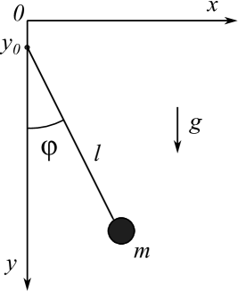
Figure 1: A pendulum oscillating in the $XOY$ plane with the suspension point moving along the axis $OY$.

For small oscillations, the coordinates of the point $m$ are:

$$x=l\sin\phi\approx l\phi,\quad y=y_{0}+l\cos\phi\approx y_{0}+l(1-{\phi}^{2}/2).$$ (8)

Here $y_{0}$ is the coordinate of the suspension point of the pendulum and $\phi$ is the deflection angle of the pendulum. The Lagrangian of the pendulum up to the terms of the first order in $\epsilon T<<1$ can be written as

$$L=\frac{ml^{2}}{2}{\dot{\phi}}^{2}-mlv\phi\dot{\phi}-\frac{ml}{2}\left(g+v\frac{\dot{l}}{l}\right){\phi}^{2},$$ (9)

where $v=\dot{y_{0}}$. Using the standard Legendre transformation and introducing the generalized momentum $p=\partial L/\partial\dot{\phi}$ instead of generalized velocity $\dot{\phi}$, we find the Hamilton function $H=p\dot{\phi}-L$,

$$H=\frac{1}{2ml^{2}}p^{2}+\frac{v}{l}p\phi+\frac{ml}{2}\left(g+\frac{v^{2}}{l}+v\frac{\dot{l}}{l}\right)\phi^{2}.$$ (10)

Thus, we directly arrive at the Hamilton (1) of the GHO, where the parameters of the Hamiltonian are given by:

$$\alpha=m(gl+v^{2}+v\dot{l}),\ \beta=v/l,\ \gamma=1/ml^{2}.$$ (11)

The second term in (10) arises due to the transition to the moving frame of reference and the lack of invariance under the spatial transformation $y\rightarrow-y$. (Such term does not appear when the suspension point of the pendulum moves only along the horizontal axis.) The renormalization of gravity $g$ in the third term of (10) is related to the action of forces emerging in the non-inertial frame of reference.

Substituting (11) into (3) and (5), we immediately obtain the adiabatic invariant,

$$I=\frac{1}{2}mg^{1/2}l^{3/2}r^{2},$$ (12)

and both (the dynamical and geometric) phases of the pendulum:

$$\Theta_{d}=\int^{t}\!\!{\sqrt{\frac{g}{l}}dt},\quad\Theta_{g}=-\int_{\Gamma}\frac{v}{2\sqrt{gl}}\left(\frac{dm}{m}+\frac{dv}{v}\right).$$ (13)

We would like to note here that the parameters $\alpha,\beta$ and $\gamma$ of the GHO play different role in determining the geometric phase. Indeed, the expression for the geometric phase in (4) does not contain the derivative of $\alpha$ with respect to $t$. By this reason we should take into account the small parameter $\dot{l}$ in $\alpha$ and in Eqs. (9) and (10), and neglect terms with such derivatives in $\beta$ and $\gamma$, if there are any. In view of the equality $\omega=\sqrt{\alpha\gamma-{\beta}^{2}}$, the expression for the dynamical phase also contains the parameter $\alpha$ and, in this way, the term with $\dot{l}$, which should obviously be included into the geometric phase $\Theta_{g}$.

As can be seen from Eqs. (10) and (13), the variation of parameter $v$ is crucial for the occurrence of the geometric phase. If the suspension point of pendulum moves with a constant speed, the geometric phase $\Theta_{g}=0$. The second term in (10) is responsible for the absence of time reversal symmetry of the system. Variations of only $l$ and $m$ cannot give rise to the geometric phase. The variation of $l$ in the second term of Eq. (10) is not enough for engendering the geometric phase because the terms proportional to the time derivative of $l$ in the second and third terms of (10) cancel each other.

Thus, we have shown the canonical equivalence of the simple linearized mathematical pendulum and the GHO with adiabatically varying parameters.

4 Damped harmonic oscillator

In the work [12] it was shown that the Hamiltonian (1) is canonically equivalent to the Hamiltonian of the equation for the dissipative harmonic oscillator:

$$\frac{1}{M}\frac{d}{dt}(M\dot{q})+2\lambda\dot{q}+{\Omega}^{2}q=0.$$ (14)

Indeed, it is easy to check that (14) follows from the Euler-Lagrange equation along with the generalized Caldirola-Kanai Lagrangian [12, 17, 18],

$$L(q,\dot{q},t)=\frac{M}{2}\exp{\left[2\int^{t}\lambda(s)ds\right]}({\dot{q}}^{2}-{\Omega}^{2}q^{2}).$$ (15)

The Lagrangian (15) makes it possible to calculate the Hamiltonian corresponding to Eq. (14):

$$H(p,q)=\frac{p^{2}}{2M}\exp{\left[-2\int^{t}\lambda(s)ds\right]}+\frac{M{\Omega}^{2}q^{2}}{2}\exp{\left[2\int^{t}\lambda(s)ds\right]}.$$ (16)

The equations known from the theory of canonical transformations,

$$p=\frac{\partial F}{\partial q},\ \ Q=\frac{\partial F}{\partial P},\ \ H(P,Q)=H(p,q)+\frac{\partial F}{\partial t},$$ (17)

establish the canonical equivalence of two different ways of describing the same Hamiltonian system. The generating function

$$F(q,P,t)=qP\exp{\left[\int^{t}\lambda(s)ds\right]},$$ (18)

and the expression (17), after the identification of the parameters

$$\alpha=M{\Omega}^{2},\ \beta=\lambda,\ \gamma=M^{-1},$$ (19)

allow us to verify the equivalence of (1) and (16) by direct calculation.

Thus, the equivalence of the plane pendulum to the GHO, on the one hand, and the GHO to the damped harmonic oscillator (DHO), on the other hand, yield the equivalence of the plane pendulum to the DHO. The last conclusion can be verified directly by the substitution

$$q=\phi\exp{\left[-\int^{t}\lambda(s)ds\right]};\,\,M=ml^{2},\ \lambda=v/l,\ {\Omega}^{2}=(gl+v^{2}+v\dot{l})l^{-2},$$ (20)

into the Lagrangian (15). As a result we obtain expression (9).

To obtain Caldirola-Kanai Lagrangian (15) of the damped oscillator we have to put

$$\phi=q\exp{\left[\int^{t}\lambda(s)ds\right]}$$ (21)

into (9) and find $\lambda$ by eliminating the term with $q\dot{q}$. This results in $\lambda=v/l$.

Thus, we have shown that the planar pendulum (9) is canonically equivalent to the dissipative DHO (14), (15). The equivalence holds for the systems with slowly varying parameters (not only for the constant ones). Another complex form of the GHO Hamiltonian, which is also canonically equivalent to the original GHO Hamiltonian (1) is presented in Appendix A.

5 Discussion

Let us expose two different points of view on the subject under discussion. Here we call them ”physical” and ”mathematical”.

The physicists believe that dissipative forces are outside of the scope of applicability of variational principles of analytical mechanics [19, 20]. The general point of view on applicability of this principle may be represented as follows (see, e.g., [21, 22]). Newtonian ’vector’ mechanics describes the motion of mechanical systems under the action of forces applied to them. Newton’s approach does not limit the nature of the forces, which are usually divided into potential and dissipative. The Lagrange-Hamilton variational mechanics describes the motion of mechanical systems under the action of only potential forces [20, 23]. From this point the existence of Lagrangian for dissipative system and its equivalence to non-dissipative one is something extraordinary. Nevertheless the Caldirola-Kanai Lagrangian describing the dissipative oscillator is not an exceptional example of ‘exotic’ systems (with the equation of motion containing the time derivatives of generalized coordinates). The Caldirola-Kanai Lagrangian also describes systems with an arbitrary potential $U(q)$ instead of $M{\Omega}^{2}q^{2}/2$ in (15).

Other example of the equation of motion and the Lagrange function for the oscillator with quadratic dependence of ‘friction’ on velocity reads [14]:

$$\ddot{q}+b{\dot{q}}^{2}+\omega^{2}q=0,$$ (22)

$$L=\frac{m}{2}\left[\left(\dot{q}^{2}-\frac{\omega^{2}}{b}q+\frac{\omega^{2}}{2b^{2}}\right)\exp{(2bq)}-\frac{\omega^{2}}{2b^{2}}\right].$$ (23)

One more example of the systems with ‘friction’ is the nonlinear Hirota oscillator playing an extremely important role in the study of nonlinear evolution equations and dynamical systems [24, 25]. Its equation of motion and the Lagrange function are

$$\ddot{\phi}+(1+{\dot{\phi}}^{2})\tan{\phi}=0,$$ (24)

$$L=\dot{\phi}\arctan{\dot{\phi}}-\frac{1}{2}\ln(1+{\dot{\phi}}^{2})+\frac{1}{2}\ln{\cos{\phi}}^{2}.$$ (25)

So, we have too many examples of equations containing the time derivatives of generalized coordinates and we should look for some explanation for this phenomenon. As a matter of fact this “strange” situation have been explained more than a century ago.

The mathematical approach [26] formulates the inverse problem of the calculus of variations as the problem of finding conditions, ensuring that a given system of differential equations of motion coincides with the system of Euler-Lagrange equations of an integral variational functional. This problem (in recent years also known as the Sonin-Douglas problem [27]) was first considered by Sonin [28] for one second order ordinary differential equation in 1886 (the almost forgotten paper). He proved that every second order equation has a Lagrangian. Then the same idea and approach appeared in 1894 [29]. Later, it was shown [26, 30] that for one-dimensional systems in context of the inverse problem of Lagrangian dynamics and non-uniqueness of Lagrangian there are infinitely many Lagrangians which result in the same trajectory in the configuration space for any second-order differential equation. They are not, of course, canonically equivalent in the usual sense, since they may very well give different second order equations for $p$ and thus different orbits in the phase space.

Different Lagrangian descriptions of the same system engender different ‘energies’, $E=\dot{q}\partial L/\partial\dot{q}-L$. It turns out that, depending on a particular choice of coordinates for its Lagrangian description, a given dynamical system may be regarded either as dissipative or not.

For $n\geqslant 2$, the Lagrangian description is generically unique [26, 31], if there is any.

More exactly the Sonin result is as follow. Any second-order differential equation,

$$\ddot{q}-F(q,\dot{q},t)=0,$$ (26)

can be presented in the Lagrangian form with the Jacobi last multiplier $\mathcal{M}$

$$\mathcal{M}\,(\ddot{q}-F(q,\dot{q},t))=0\quad\Leftrightarrow\quad\frac{d}{dt}\frac{\partial L}{\partial\dot{q}}-\frac{\partial L}{\partial q}=0.$$ (27)

The multiplier $\mathcal{M}(q,\dot{q},t)$ satisfies the following equation

$$\frac{\partial\mathcal{M}}{\partial t}+\dot{q}\frac{\partial\mathcal{M}}{\partial q}+\frac{\partial\mathcal{M}F(q,\dot{q},t)}{\partial\dot{q}}=0.$$ (28)

After finding multiplier $\mathcal{M}$, the Lagrangian can be get from the equation

$$\frac{\partial^{2}\mathcal{L}}{\partial\dot{q}^{2}}=\mathcal{M}.$$ (29)

It is easy to verify that equations (14) (with constant parameters), (22) and (25) have the following multipliers $M\exp(2\lambda t),\,m\exp(-2bq)$ and $1/(1+\dot{\varphi}^{2})$ correspondingly.

So, in this way, from the mathematical viewpoint of the Lagrangian and Hamiltonian approaches, there is nothing paradoxical in the fact that the same Hamiltonian system, the generalized harmonic oscillator in our case, is canonically equivalent to the two different systems: the usual plane mathematical pendulum and the damped harmonic oscillator. Nevertheless, in some physical scientific circles there is still a popular belief that the Lagrangian and Hamiltonian approaches are not suitable for the consideration of dissipative systems. Unfortunately, this point of view is deeply rooted and many authors keep on inventing new formulations of the principle of the least action (e.g., [22, 32]).

6 Conclusion

We studied the motion of planar linearized mathematical pendulum with slowly varying parameters (the mass, the length of the suspension string and the speed of the suspension point). The Hamiltonian of the pendulum was cast into the form of the Hamiltonian for the GHO. Thus, we give the example of the simple Hamiltonian system described by the equations of the GHO. The paradoxical feature of the result is that the same Hamiltonian system, the GHO in this case, can be canonically equivalent to the two different systems, to the planar mathematical pendulum (the Hamiltonian system) and to the damped harmonic oscillator (the dissipative system with time dependent Lagrangian). This observation disputes the separation of dynamical systems into two classes of the dissipative and Hamiltonian ones. In our opinion the dividing line might be, for example, between the systems which are invariant and non-invariant with respect to the time reversal transformation.

Appendix A

Another convenient form of Hamiltonian (1) is its complex form ${\cal H}^{z}$. It can be obtained after changing the variables $Q$ and $P$ by $z$ and $\overline{z}$.

$$Q=\sqrt{{\gamma\over{2\omega}}}(z+\overline{z}),\ \ \ \ \ P={1\over\sqrt{2\omega\gamma}}\big{[}(i\omega-\beta)z-(i\omega+\beta)\overline{z}\big{]}\ .$$ (30)

The generating function $F(Q,z)$ of the transformation $(P,Q)\to(-i\overline{z},z)$ is get by integration of the equations $\displaystyle{{{\partial F}\over{\partial Q}}=P(Q,z)}$ and ${\displaystyle{{\partial F}\over{\partial z}}=i\overline{z}}(Q,z)$ deduced from the differential identity characterizing a canonical transformation

$$PdQ-Hdt=-i{\overline{z}}dz-{\cal H}^{z}dt+dF\ .$$ (31)

Taking into account the relations (30) one gets

$$F(Q,z)=-{{i\omega+\beta}\over{2\gamma}}Q^{2}+i\sqrt{\frac{2\omega}{\gamma}}Qz-{1\over 2}iz^{2}\ .$$ (32)

The Hamiltonian ${\cal H}^{z}$ for the new conjugate variables $(-i\overline{z},z)$ is then obtained from the relation $\displaystyle{{\cal H}^{z}=H+{\partial F\over\partial t}}$ . Its expression reads

$${\cal H}^{z}=\omega z\overline{z}+{{i\dot{\omega}}\over{4\omega}}(z^{2}-\overline{z}^{2})-{{\dot{\beta}}\over{4\omega}}(z+\overline{z})^{2}+{{\dot{\gamma}}\over{4\omega\gamma}}[-i\omega(z^{2}-\overline{z}^{2})+\beta(z+\overline{z})^{2}].$$ (33)

One can verify that the Hamilton equations

$$\dot{z}={{\partial{\cal H}^{z}}\over{\partial(-i\overline{z})}}\ \ ,\ \ -i\dot{\overline{z}}=-{{\partial{\cal H}^{z}}\over{\partial z}}\$$ (34)

indeed give correct equations for $z$ and the corresponding one for $\overline{z}$ after substitution (30) in (6). Conservation of the Poisson brackets $\{Q,P\}_{QP}=\{Q,P\}_{z,-i\overline{z}}=1$ of the transformations (30) manifests about their canonicity.

The multiplier $\omega-{{\dot{\beta}}/{2\omega}}+{{\dot{\gamma}\beta}/{2\omega\gamma}}$ of the term $z\overline{z}$ in Eq. (33) gives once again the result (4).

Appendix B

The other way to obtain the adiabatic invariant and phases is as follow. After presenting the term $mlv\phi\dot{\phi}$ in the Lagrangian (9) in the form $(1/2)d(mlv\phi^{2})/dt-(\phi^{2}/2)d(mlv)/dt$ and neglecting the total derivative $(1/2)d(mlv\phi^{2})/dt$, we get

$$L=\frac{ml^{2}}{2}{\dot{\phi}}^{2}-mgl\left[1-\frac{v}{g}\left(\frac{\dot{m}}{m}+\frac{\dot{v}}{v}\right)\right]\frac{{\phi}^{2}}{2},$$ (35)

where we can immediately identify the squared frequency,

$$\omega_{pend}^{2}=\frac{g}{l}\left[1-\frac{v}{g}\left(\frac{\dot{m}}{m}+\frac{\dot{v}}{v}\right)\right].$$ (36)

More rigorously, using Eqs. (35) or (9), we should write the Euler-Lagrange equation and look for its solution in the form $\phi=r\cos\Theta$. Neglecting quantities of the second order of $\epsilon$, we obtain simple differential equations of the first order for $r$ and $\Theta$ containing first derivatives of the parameters. The solutions of these equations yield (12) and (13).

References

References

- [1] F. Wilczek, A. Shapere, Geometric Phases in Physics, World Scientific, 1989.
- [2] S.I. Vinitskii, V.L. Derbov, V.M. Dubovik, B.L. Markovski, Yu.P. Stepanovskii, Topological phases in quantum mechanics and polarization optics, Sov. Phys. Usp. 33(6) (1990) 403-428.
- [3] D.N. Klyshko, Berry geometric phase in oscillatory processes, Phys. Usp. 36(11) (1993) 1005-1019.
- [4] G.B. Malykin, S.A. Kharlamov, Topological phase in classical mechanics, Phys. Usp. 46 (2003) 957-965.
- [5] D. Chruscinski, A. Jamiolkowski, Geometric Phases in Classical and Quantum Mechanics, Springer Science and Business Media, 2004.
- [6] M.V. Berry, Quantal Phase Factors Accompanying Adiabatic Changes, Proc. Roy. Soc. A392 (1984) 45-57.
- [7] J.H. Hannay, Angle variable holonomy in adiabatic excursion of an integrable Hamiltonian, J. Phys. A: Math. Gen. 18 (1985) 221-230.
- [8] M.V. Berry, Classical adiabatic angles and quantal adiabatic phase, J. Phys. A: Math. Gen. 18 (1985) 15-27.
- [9] A.M. Dykhne, Quantum Transitions in the Adiabatic Approximation, Soviet Physics JETP 11 (1960) 411-415.
- [10] M.V. Fedoruk, Asymptotic Analysis: Linear Ordinary Differential Equations, translated from the Russian by Andrew Rodick, Springer, Berlin, New York, 1993.
- [11] K.Yu. Bliokh, The appearance of a geometric-type instability in dynamic systems with adiabatically varying parameters, J. Phys. A: Math. Gen. 32 (1999) 2551-2565.
- [12] O.V. Usatenko, G.P. Provost, G. Vallee, A Comparative study of the Hannay’s angles associated with a damped harmonic oscillator and a generalized harmonic oscillator, J. Phys. A: Math. Gen. 29 (1996) 2607-2610.
- [13] M. Razavy, Classical and Quantum Dissipative Systems, Imperial College Press, 2006.
- [14] C.E. Smith, Lagrangians and Hamiltonians with friction, Journal of Physics: Conference Series 237 (2010) 012021.
- [15] D.H. Kobe, J. Zhu, Generalized Hanney angle for the most general time-dependent harmonic oscillator, Int. J. Mod. Phys. B 07 (1993) 4827-4840.
- [16] A.A. Slutskin, Motion of a one-dimensional nonlinear oscillator under adiabatic conditions, Soviet Physics JETP 18 (1964) 676.
- [17] P. Caldirola, Forze non conservative nella meccanica quantistica, Nuovo Cimento 18 (1941) 393-400.
- [18] E. Kanai, On the quantization of dissipative systems, Prog. Theor. Phys. 3 (1948) 440-442.
- [19] L.D. Landau, E.M. Lifshits, Mechanics, Butterworth-Heinemann, 1976.
- [20] C. Lanczos, Variational principles of mechanics, Dover publications, Inc. New York, 1986.
- [21] V.E. Tarasov, Quantum dissipative systems I. Canonical quantization and quantum Liouville equation, Theoretical and mathematical physics 100 (1994) 402-417.
- [22] V.E. Tarasov, Quantum mechanics of non-Hamiltonian and dissipative systems, Elsevier Science, 2008.
- [23] H. Goldstein, Classical mechanics, 3rd ed., Pearson Education Lim., 2014.
- [24] R. Hirota, Exact N-Soliton Solution of Nonlinear Lumped Self-Dual Network Equations, J. Phys. Soc. Jpn. 35 (1973) 289-294.
- [25] D.V. Laptev, Classical Energy Spectrum of the Hirota Nonlinear Oscillator, J. Phys. Soc. Jpn. 82 (2013) 044005.
- [26] G. Morandi, C. Ferrario, G.Lo. Vecchio, G. Marmo, C. Rubano, The inverse problem in the calculus of variations and the geometry of the tangent bundle, Physics Reports 188 (1990) 147-284.
- [27] Zenkov, D. (ed.): The Inverse Problem of the Calculus of Variations, Local and Global Theory. Atlantis Press, Amsterdam (2015).
- [28] N. J. Sonin, About determining maximal and minimal properties of plane curves, Warsawskye Universitetskye Izvestiya (1886) (1-2), 1-68 (in Russian); English translation by R. Matsyuk, Lepage Inst. Archive, No. 1 (2012), 1-42.
- [29] Darboux, G.: Lecons sur la theorie generale des surfaces. Gauthier-Villars, Paris (1894)
- [30] D.G. Currie and E.J. Saletan, q-Equivalent Particle Hamiltonians. I. The Classical One-dimensional Case, J. Math. Phys. 7 (1966) 967-974.
- [31] Douglas, J.: Solution of the inverse problem of the calculus of variations. Trans. AMS 50, 71-128 (1941).
- [32] C.G. Galley, Classical Mechanics of Nonconservative Systems, Phys. Rev. Lett. 110 (2013) 174301.