Estimated values of the kinetic energy for liquid ³He

Abstract

The kinetic energy is estimated for the ground-state of liquid ³He at equilibrium density. The obtained value for this quantity, $10.16\pm 0.05$ K/atom at density $0.0163~{}\mbox{\AA}^{-3}$, is in agreement with most of the experimental data found in the literature. This result resolves a long-standing controversy between experimental and theoretical values of this quantity. The variational path integral method, an“exact” quantum Monte Carlo method extended for fermionic systems, is applied in the calculations. The results obtained are subjected only to the restrictions imposed by a chosen nodal structure without any further approximation, even for quantities that do not commute with the Hamiltonian. The required fixed-node approximation entails an implementation that allows a more effective estimation of the quantities of interest. Total and potential energies together with the radial distribution function are also computed.

We investigated properties of normal condensed ³He at the equilibrium density and compared to experimental values. Neither experimental or theoretical quantities of this system are easily obtained. Direct experimental information about single-particle dynamical properties such as the mean kinetic energy $\langle E_{K}\rangle$ Bryan et al. (2016); Dimeo et al. (1998); Azuah et al. (1995); Mook (1985); Sokol et al. (1985) of this strongly interacting Fermion system can be obtained by deep inelastic neutron scattering. These are challenging experiments since the absorption cross-section for thermal neutrons is about three orders of magnitude higher than for inelastic scattering. On the other hand, theories using quantum Monte Carlo many-body methods must avoid the Fermion sign problem that so far has resisted an entirely satisfactory answer. Most of the experiments report kinetic energies in the range of 8 to 11 K/atom Bryan et al. (2016); Dimeo et al. (1998); Azuah et al. (1995); Mook (1985); Sokol et al. (1985), whereas theory predicted values between 12 and 13 K/atom Mazzanti et al. (2004); Moroni et al. (1997); Manousakis et al. (1983). This is a small, but a significant difference for an “exact” method.

In calculations made at zero temperature, we employed the variational path integral (VPI) method introduced by Ceperley Ceperley (1995), who computed the total energy of ⁴He at equilibrium density. This is a well established method, also known as path-integral ground-state (PIGS), employed in the recent investigation of a variety of bosonic systems, see for instance references Rossoti et al., 2017; Abolins et al., 2018; Bertaina et al., 2016. We extended the method to deal with fermionic systems, in order to estimate properties of liquid ³He. In this approach, a projection to the ground-state of the system is made from a given initial state using ideas of path-integrals over imaginary time Ceperley (1995). The employed projector and how it is used in the VPI method is reminiscent of how particles are treated in a path-integral Monte Carlo calculation. The necklace describing a particle can be thought of as having been cut and the coordinates at the extremities are assumed to be those of a trial function. This is what we refer to as an open path or polymer. Configurations associated to monomers at the middle of long enough polymers allow one to estimate any quantity, regardless whether their expected values are associated to operators that do or do not commute with the Hamiltonian. “Exact” values are always obtained without the need for any extrapolation. However, since we are dealing with a fermionic system, the usual fixed-node approximation needs to be used. In our context, configurations associated to the trial function at each end of the polymers need to be considered. Results obtained for all quantities of interest are only subjected to the restrictions imposed by a chosen nodal structure.

Our main aim is the investigation of properties of liquid ³He associated with operators that do not commute with the Hamiltonian. We especially want to study the kinetic energy of these systems, since there are controversies between experimental and theoretical results that continue up until the present Bryan et al. (2016). We show that the VPI method gives estimates that are in agreement with most of the experimental results.

Ground-state properties estimated by the VPI method are made by applying the imaginary time evolution operator, $\rho(\beta)=\exp\left(-\beta{\cal H}\right)$, with ${\cal H}$ being the system Hamiltonian, in an initial state $\ket{\Psi_{T}}$ to project out the ground-state $\ket{\phi_{0}}$. The state $\ket{\phi(\beta)}=\rho(\beta)\ket{\Psi_{T}}$ converges exponentially to $\ket{\phi_{0}}$ as $\beta$ increases.

The matrix element $\rho(R,R^{\prime},\beta)=\bra{R}\rho(\beta)\ket{R^{\prime}}$, propagates configuration $R$ to $R^{\prime}$ in a “time” $\beta$ Ceperley (1995), where $R$ stands for all particle coordinates. It is written as the exponential of the action integrated over all paths. The integration can be made by factorizing $\rho(\beta)$ into the product of $M$ projectors $\rho(\tau)$, $\tau=\beta/M$, and using the convolution property

$$\rho(R,R^{\prime},\beta)= \displaystyle\int dR_{1}\ldots dR_{M-1}\rho(R,R_{1},\tau)$$

$$\times\rho(R_{1},R_{2},\tau)\ldots\rho(R_{M-1},R^{\prime},\tau).$$

The intermediary configurations or beads $R_{n}$, $n=1,\ldots,M-1$, can be seen as the set of atomic coordinates at “time” $t=n\tau$. The beads stand for a sort of discretization of the path from $R$ to $R^{\prime}$ in a “time” $\beta$. Therefore the integration of Eq.(Estimated values of the kinetic energy for liquid ³He) converges to the integration over all paths if $\tau$ is small enough. In this case, it is possible to employ the primitive approximation,

$$\rho(R^{\prime\prime},R^{\prime\prime\prime},\tau)\approx\rho_{0}(R^{\prime\prime},R^{\prime\prime\prime},\tau)e^{-\frac{\tau}{2}\left[V(R^{\prime\prime})+V(R^{\prime\prime\prime})\right]},$$ (2)

where $V(R)$ is the potential energy of configuration $R$, and $\rho_{0}(R^{\prime\prime},R^{\prime\prime\prime},\tau)$ is the projector of non-interacting atoms, $\rho_{0}(R^{\prime\prime},R^{\prime\prime\prime},\tau)\propto\exp[-(R^{\prime\prime}-R^{\prime\prime\prime})^{2}/4\lambda\tau]$, where $\lambda$ is $\hbar^{2}/2m$. The primitive approximation is accurate to the second order in $\tau$. We also implemented calculations with the Suzuki pair approximation Cuervo et al. (2005); Rossi et al. (2009), which is a fourth order in $\tau$ approximation,

$$\rho(R_{k},R_{l},\tau)\approx\rho_{0}(R_{k},R_{l},\tau)\displaystyle\prod_{i<j}e^{-U(r^{(k)}_{ij},r^{(l)}_{ij})},$$ (3)

$r^{(\cdot)}_{ij}$ is the relative distance between atoms $i$ and $j$ within configuration $R_{\cdot}$, if $k$ is even

$$U(r^{(k)},r^{(l)})=\frac{\tau}{3}\left[2v(r^{(k)})+v(r^{(l)})\right]+$$ (4)

$$\frac{\tau^{3}\lambda}{9}\left[\frac{\partial v}{\partial r}(r^{(k)})\right]^{2},$$

and if $k$ is odd then $U(r^{(k)},r^{(l)})=(\tau/3)[v(r^{(k)})+2v(r^{(l)})]$; $v(r)$ is the inter-atomic potential.

By substituting Eq.(2) or Eq.(3) into Eq.(Estimated values of the kinetic energy for liquid ³He) we obtain a formula for $\rho(R,R^{\prime},\beta)$. Any error introduced by one of these approximations can, in general, be made smaller than the statistical uncertainties of the Monte Carlo method. The choice of Eq.(2) or Eq.(3) did not affect our results.

In a system made of identical Fermions such as the one we are interested in, the expression for $\rho(R,R^{\prime},\beta)$ needs to be anti-symmetric under the permutation of any pair of particles in the configuration $R$Ceperley (1995, 1996). However, if $\Psi_{T}(R)$ is anti-symmetric, it is possible to incorporate the minus sign rising from odd permutations in $\rho(R,R^{\prime},\beta)$ into $\Psi_{T}(R)$ since

$$\rho(R,R^{\prime},\beta)\Psi_{T}(R^{\prime})=$$ (5)

$$(-1)^{n_{p}}\rho(R,{\cal P}R^{\prime},\beta)\Psi_{T}(R^{\prime})=$$

$$\rho(R,{\cal P}R^{\prime},\beta)\Psi_{T}({\cal P}R^{\prime}),$$

where ${\cal P}$ changes the coordinates of $n_{p}$ particles in a given configuration. And so, after integration in $R^{\prime}$, all permutation will have the same result (more details will be given elsewhere).

Any property of the system in its ground-state can be estimated in a straightforward manner. If a given property is associated to an operator ${\cal O}$, its expected value can be written as

$$O(\beta) \propto\bra{\phi(\beta)}{\cal O}\ket{\phi(\beta)}$$ (6)

$$=\bra{\Psi_{T}}\rho(\beta){\cal O}\rho(\beta)\ket{\Psi_{T}},$$

or as

$$O(\beta)=\int dR_{1}\ldots dR_{2M+1}P(R_{1},\ldots,R_{2M+1})O_{L}^{{\cal X}},$$ (7)

in terms of the probability distribution function $P$ of a given path

$$P(R_{1},\ldots,R_{2M+1}) \propto\Psi_{T}(R_{1})\rho(R_{1},R_{2},\tau)\ldots$$ (8)

$$\times\ldots\rho(R_{2M},R_{2M+1},\tau)\Psi_{T}(R_{2M+1}).$$

In Eq. (7), $O_{L}^{{\cal X}}(R_{.})$ is the local value of the operator at a given bead and the index ${\cal X}$ labels different estimators this method can allow us to use. If ${\cal O}$ commutes with the Hamiltonian, by using its coordinate representation it is possible to estimate its value for a given configuration $R$ at the end of the path through $O_{L}^{{\cal E}}(R)={\cal O}\Psi_{T}(R)/\Psi_{T}(R)$. This is the local value of $\cal O$ evaluated for configurations at the end of the path associated to $\Psi_{T}(R)$.

An estimate of the “exact” average value of ${\cal O}$, even if it does not commute with the system Hamiltonian, can be obtained through the so called direct estimator given in the coordinate representation by $O_{L}^{{\cal D}}(R_{i},R_{i+1})={\cal O}\rho(R_{i},R_{i+1},\tau)/\rho(R_{i},R_{i+1},\tau)$, applied at the polymer middle. For efficiency, the best approach is to consider the average value $O_{L}^{{\cal D}}(R_{i},R_{i+1})$ for $i=M$ and $i=M+1$.

For the total and kinetic energy estimates, we can also use the thermodynamic estimators $O^{\cal T}_{L}$ to consider configurations at the middle of the polymer. In this context, derivatives of $\rho(\beta)$ with respect to $\beta$ and the mass $m$ are associated with the total and kinetic energy respectively Ceperley (1995). For any of these estimators, care must be taken when utilizing the Suzuki pair approximation of Eq.(3), since the operators must be inserted in odd beads Rossi et al. (2009).

Since we want to investigate fermionic systems the probability density given by Eq.(8) can be negative. This is the sign problem common to most of the ground-state Monte Carlo methods for fermionic systems. Here we avoid this problem by rejecting sampled paths where $\Psi_{T}(R_{1})\Psi_{T}(R_{2M+1})<0$. This is a fixed-node approximation that has more degrees of freedom than the restriction $\Psi_{T}(R)>0$ imposed when one applies an importance function transformation to sample $\phi_{0}(R)\Psi_{T}(R)$, where $\phi_{0}(R)$ is unknown. We believe that the extra degrees of freedom we have in this instance improves the exploration of the configuration space, especially to regions where the nodal structure of $\Psi_{T}(R)$ is not identical to that of the ground-state.

The system we consider is made of $N$ atoms of ³He inside a cubic box with periodic boundary conditions applied to the faces of the box. In our model, the atoms interact through the well-tested pairwise potential $v(r)$, HFD-B3-FCI1 Aziz et al. (1995), and the Hamiltonian can be written as,

$${\cal H}=\frac{1}{2m}\displaystyle\sum_{i=1}^{N}{\mathbf{p}}_{i}^{2}+\displaystyle\sum_{i<j}^{N}v(r_{ij}),$$ (9)

where $m$ is the ³He mass, ${\mathbf{r}}_{i}$ and ${\mathbf{p}}_{i}$ are respectively the coordinates and the momentum associated to a $i$-th atom and $r_{ij}=|{\mathbf{r}}_{i}-{\mathbf{r}}_{j}|$.

It is interesting to experiment with different trial functions at the end of the polymer. This allows us to investigate the convergence behavior towards the exact ground-state of the quantities of interest. In this way, two wave functions with different degrees of superposition with the ground-state were considered. We performed two series of independent runs, one for each of the functions used at the extremities of the polymer. The simplest function we have considered at the extremities was the Jastrow-Slater (JS) wave function,

$$\Psi_{T}(R)=e^{-\frac{1}{2}\sum_{i<j}u(r_{ij})}\times$$ (10)

$${\rm det}_{\uparrow}\left(e^{i{\mathbf{k}}_{l}\cdot{\mathbf{r}}_{m}}\right){\rm det}_{\downarrow}\left(e^{i{\mathbf{k}}_{l}\cdot{\mathbf{r}}_{n}}\right),$$

where $u(r)=(b/r)^{5}$. The nodal structure of this wave function was improved by adding backflow correlations in the Slater determinantSchmidt et al. (1981); Panoff and Carlson (1989). These correlations are introduced by a change in the particle coordinates, ${\mathbf{r}}_{.}\rightarrow{\mathbf{r}}_{.}+\sum_{j\neq\cdot}\eta(r_{\cdot j})(\mathbf{r}_{.}-\mathbf{r}_{j})$, of the Slater determinant, where

$$\eta(r)=\lambda_{B}e^{-\left(\frac{r-s_{B}}{w_{B}}\right)^{2}}+\frac{\lambda_{B}^{\prime}}{r^{3}}.$$ (11)

and $\lambda_{B},\ s_{B},\ w_{B},\ \lambda_{B}^{\prime}$ are parameters. Three-body correlationsSchmidt et al. (1981); Panoff and Carlson (1989) were also introduced at the extremities of the open path. Its functional form is given by

$$\exp\left[-\frac{1}{2}\sum_{i<j}\tilde{u}(|\mathbf{r}_{i}-\mathbf{r}_{j}|)-\frac{\lambda_{T}}{4}\sum_{l}\mathbf{G}(l)\cdot\mathbf{G}(l)\right],$$ (12)

where $\mathbf{G}(l)=\sum_{i\neq l}\xi(r_{ij})\mathbf{r}_{ij}$,

$$\xi(r)=e^{-\left(\frac{r-s_{T}}{w_{T}}\right)^{2}}.$$ (13)

and $s_{T},\ w_{T}$ are parameters. The pseudopotential $\tilde{u}(r)=u(r)-\lambda_{T}\xi^{2}(r)r^{2}$ cancels two-body factors arising from $\mathbf{G}(l)$. We refer to this improved wave function as JS+BF+T. In order for the wave function to be periodic it is required that the correlation functions and its derivatives go smoothly to zero at half of the side of the simulation box, $L$. This can be achieved by the replacement $f(r)\rightarrow f(r)+f(L-r)-2f(L/2)$, where $f$ is either $u$, $\eta$ or $\xi$.

Our calculations were performed with $N=54$ atoms in a non-polarized system at the equilibrium density, $0.0163\ \mbox{\AA}^{-3}$. The sampling of the beads were made by the multi-Metropolis algorithm described in reference Ceperley (1995). The configurations at the extremities of the path were sampled with the usual Metropolis algorithm.

The total energy as a function of $\beta$, $H(\beta)$, was calculated using the estimator at the end of the path for the two different trial wave functions, see Fig. 1. As $\beta$ increases the energy decreases, almost exponentially, creating a sequence of upper bound values to the ground-state energy. The results show that improvements to the trial wave function due to backflow and three-body correlations accelerate the convergence to the ground-state of the system. The ground-state energy itself can only be achieved if the nodal structure of $\Psi_{T}(R)$ is identical to that of the ground-state. In this sense the improvement in the nodal structure of $\Psi_{T}(R)$ is noticeable due to the addition of backflow correlations.

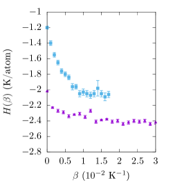
Figure 1: Total energy $H(\beta)$ calculated with the estimator at the end of the path. The points at $\beta=0\ \text{K}^{-1}$ correspond to variational energies. Squares represent the calculations with the JS wave function and triangles stand for calculations using the JS+BF+T function. The parameters for this wave function are $b=2.99\ \mbox{\AA}$, $\lambda_{B}=-0.14$, $\lambda_{B}^{\prime}=-0.15$, $s_{B}=1.89\ \mbox{\AA}$, $w_{B}=1.38\ \mbox{\AA}$, $\lambda_{T}=-1.8$, $s_{T}=1.69\ \mbox{\AA}$ and $w_{T}=1.28\ \mbox{\AA}$.

The tail ($\beta\geq 1.5\times 10^{-2}$ K^-1) of the curve in Fig. 1 associated to the JS+BF+T wave function was fitted to a constant straight line resulting in a total energy of $-2.41\pm 0.01$ K/atom, which is a very good upper bound to the experimental data $-2.47\pm 0.01$ K/atom Roberts et al. (1964). From now on, all results we report are in reference to the results obtained from the wave function above.

For the estimation of the kinetic energy we use the same procedure of considering all the converged values we have obtained for this quantity. The straight line fit to these results gave us the value we adopt for the ground-state kinetic energy, $10.16\pm 0.05$ K/atom. In Fig. 2, we plotted this value together with experimental data from the literature for liquid ³He at equilibrium density. Most of the experimental data lies in a range from $8$ to $11$ K/atom, which is in excellent agreement with our estimates, thus resolving a long-standing disagreement between experimental data and theoretical Monte Carlo calculations For completeness in Table 1, we give values of the potential and kinetic energies calculated with the direct and thermodynamic estimators.

Table 1: Kinetic and potential energies in units of K/atom evaluated with the direct $(\cal D)$ and thermodynamic $(\cal T)$ estimators using configurations projected from the JS+BF+T wave function.

Estimator	Kinetic Energy	Potential Energy
${\cal D}$	$10.19\pm 0.07$	$-12.75\pm 0.01$
${\cal T}$	$10.14\pm 0.07$	$-12.75\pm 0.01$

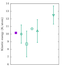
Figure 2: Comparison of our results for the kinetic energy of ³He at the equilibrium density obtained with projections of configurations from the JS+BF+T wave function, and experimental data from the literature. The symbols were horizontally displaced for the sake of clarity. The full square stands for our calculation; this symbol size is larger than the statistical uncertainty. The experimental data are plotted with empty symbols: square Sokol et al. (1985), circle Mook (1985), up triangle Azuah et al. (1995) down triangle Bryan et al. (2016), and rhombus Dimeo et al. (1998).

We have also calculated the radial distribution of atoms and its spin-resolved components for atoms with parallel and anti-parallel spins. These quantities were calculated with the direct estimator, see Fig. 3. The anti-parallel spin curve has a more pronounced peak because atoms with different spins do not suffer the Pauli exclusion.

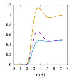
Figure 3: Radial distribution function of liquid ³He at equilibrium density. The total radial distribution function is represented by the dashed-and-dotted line; the spin-resolved distribution functions for spin parallel and spin anti-parallel atoms are represented by the solid and dashed lines respectively.

In summary, as we have shown, the VPI approach to study the ground-state of fermionic systems is robust and reliable. Any quantity, associated with operators that do or do not commute with the Hamiltonian is readily estimated without the need of extrapolations. By avoiding them, estimates can be obtained completely free from any possible bias introduced by variational calculations. Moreover, a long-standing disagreement between experimental data and theoretical calculations of the ground-state kinetic energy was resolved. To what degree the findings in this work will be reflected in other systems is still an open question. Nevertheless, this question is very important, because many results for physical properties of great interest were obtained in the literature using extrapolations. Acknowledgments: The authors acknowledge financial support from the Brazilian agencies Fundação de Amparo à Pesquisa do Estado de São Paulo (FAPESP) and Conselho Nacional de Desenvolvimento Científico e Tecnológico (CNPq). Part of the computations were performed at the Centro Nacional de Processamento de Alto Desempenho em São Paulo (CENAPAD-SP).

References

- Bryan et al. (2016) M. S. Bryan, T. R. Prisk, R. T. Azuah, W. G. Stirling, and P. E. Sokol, EPL 115, 6601 (2016).
- Dimeo et al. (1998) R. M. Dimeo, P. E. Sokol, R. T. Azuah, S. M. Bennington, W. G. Stirling, and K. Guckelsberger, Physica B 241-243, 952 (1998).
- Azuah et al. (1995) R. T. Azuah, W. G. Stirling, K. Guckelsberger, R. Scherm, S. M. Bennington, M. L. Yates, , and A. D. Taylor, J. Low Temp. Phys. 101, 951 (1995).
- Mook (1985) H. A. Mook, Phys. Rev. Lett. 22, 2452 (1985).
- Sokol et al. (1985) P. E. Sokol, K. Sköld, D. L. Price, and R. Kleb, Phys. Rev. Lett. 54, 909 (1985).
- Mazzanti et al. (2004) F. Mazzanti, A. Polls, J. Boronat, and J. Casulleras, Phys. Rev. Lett. 92, 085301 (2004).
- Moroni et al. (1997) S. Moroni, G. Senatore, and S. Fantoni, Phys. Rev. B 55, 1040 (1997).
- Manousakis et al. (1983) E. Manousakis, S. Fantoni, V. R. Pandharipande, and Q. N. Usmani, Phys. Rev. B 28, 3770 (1983).
- Ceperley (1995) D. M. Ceperley, Rev. Mod. Phys. 67, 279 (1995).
- Rossoti et al. (2017) S. Rossoti, M. Teruzzi, D. Pini, D. E. Galli, and G. Bertaina, Phys. Rev. Lett. 119, 215301 (2017).
- Abolins et al. (2018) B. P. Abolins, R. E. Zillich, and K. B. Whaley, J. Chem. Phys. 148, 102338 (2018).
- Bertaina et al. (2016) G. Bertaina, M. Motta, M. Rossi, E. Vitali, and D. Galli, Phys. Rev. Lett. 116, 135302 (2016).
- Cuervo et al. (2005) J. E. Cuervo, P.-N. Roy, and M. Boninsegni, J. Chem. Phys. 122, 114504 (2005).
- Rossi et al. (2009) M. Rossi, M. Nava, L. Reatto, and D. E. Galli, J. Chem. Phys. 131, 154108 (2009).
- Ceperley (1996) D. Ceperley, in Monte Carlo and Molecular Dynamics of Condensed Matter Systems (1996).
- Aziz et al. (1995) R. A. Aziz, A. R. Janzen, and M. R. Moldover, Phys. Rev. Lett. 74, 1586 (1995).
- Schmidt et al. (1981) K. E. Schmidt, M. A. Lee, M. H. Kalos, and G. V. Chester, Phys. Rev. Lett. 47, 807 (1981).
- Panoff and Carlson (1989) R. M. Panoff and J. Carlson, Phys. Rev. Lett. 62, 1130 (1989).
- Roberts et al. (1964) T. R. Roberts, R. H. Sherman, and S. G. Sydoriak, J. Res. Natl. Bur. Stand. 68A, 567 (1964).