Mathematical model with autoregressive process for electrocardiogram signals

Abstract

The cardiovascular system is composed of the heart, blood and blood vessels. Regarding the heart, cardiac conditions are determined by the electrocardiogram, that is a noninvasive medical procedure. In this work, we propose autoregressive process in a mathematical model based on coupled differential equations in order to obtain the tachograms and the electrocardiogram signals of young adults with normal heartbeats. Our results are compared with experimental tachogram by means of Poincaré plot and dentrended fluctuation analysis. We verify that the results from the model with autoregressive process show good agreement with experimental measures from tachogram generated by electrical activity of the heartbeat. With the tachogram we build the electrocardiogram by means of coupled differential equations.

1 Introduction

The cardiovascular system (CVS) is responsible for supplying the human organs with blood. It is composed by the heart, the arteries, and the veins. The heart has as function to pump blood throughout the body, that is realised by means of contractions [1]. The human heart beats an average $72$ beats per minute and pumps 0.07 liters of blood per beat [2, 3]. The contraction and relaxation of the heart is obtained by a single cycle of the electrocardiogram signal (ECG), namely the ECG records of the electrical activity of the heart. Waller in 1887 [4] measured for the first time the electrical activity from the heart, and the first practical electrocardiograph was invented by Einthoven in 1901 [5] that it was used as a tool for the diagnosis of cardiac abnormalities.

In the recent past, several theoretical investigations pertaining to CVS have been carried out to analyse electrocardiogram signal [6, 7, 8]. Mathematical models have been developed to understand physiological function and disfunction in CVS. A mathematical model which have been used to generate ECG signals is the Van der Pol oscillator [9]. Gois and Savi considered three modified Van der Pol oscillators connected by time delay coupling to describe heart rhythm behaviour [10]. The coupled Van der Pol oscillators was also used in studies about the control of irregular behaviour in pathological heart rhythms [11]. McSharry and collaborators [12] introduced a dynamical model to describe generating synthetic electrocardiogram signals. This model is based on a set of three ordinary differential equations in that it is incorporated the respiratory sinus arrhythmia (RSA) by means of a bimodal power spectrum consisting of the sum of two Gaussian distributions.

In this work, instead two Gaussian distributions we propose an autoregressive (AR) process for the RSA to obtain the tachograms and, consequently, the ECGs of young adults with normal heartbeats. AR model can be used to quantify gains and delays by which cardiac interval, lung volume, blood pressure and sympathetic activity affect each other [13]. Cardiologists utilise AR model when they are interested in fit tachograms through mathematical regressions softwares. The tachogram is a signal that allows the study of heart rate variability (HRV) [14, 15]. Boardman and collaborators [16] study autoregressive model for the HRV. They found the optimum order of autoregressive model which can be used for spectral analysis of short segments of tachograms. We compare the results obtained from two Gaussian distributions and AR process with experimental tachograms of healthy young adults. To do that, we use as diagnostic tools the Poincaré plot [17] and detrended fluctuation analysis (DFA) [18]. We have verified that the result with AR process agrees with the experimental tachogram more closely than the result with two Gaussian distributions. This way, we generate the ECG by means of coupled differential equations considering the AR process to obtain the tachogram and the frequency of the ECG. The frequency is an important parameter in the mathematical model for the ECG signal, and variation in the frequency produces variation in the times elapsed between successive heartbeats.

This article is organised as follows: in Section 2 we introduce the ECG model with autoregressive process for tachograms, in Section 3 we compare our results with experimental data, and in the last Section we draw our conclusions.

2 The mathematical model

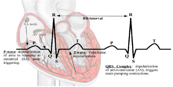
Figure 1: (Colour online) ECG following a normal hearbeat.

The ECG is a noninvasive method used to measure electrical activity of the heart through electrodes placed on the surface of the skin. Figure 1 shows the relationship between the cardiac conduction and the ECG. In the sinoatrial node (SA), known as natural pacemaker, the heartbeat starts. The atrioventricular node (AV) is responsible for the passage of electrical signals from the atria to the ventricles. At last, the signal arrives at the Purkinje fibers and makes the heart contract to pump blood, where the R-peak occurs. The time between successive R-peaks is the RR-interval and the series of RR-intervals is known as RR tachogram.

McSharry and collaborators [12] argued that the heartbeat can be described by means of three coupled ordinary differential equations with the inclusion of RSA at the high frequencies ($f_{\rm RSA}$) and Mayer waves (MW) at the low frequencies ($f_{\rm MW}$). The equations are given by

$${\dot{x}} = \alpha x-\omega y,$$

$${\dot{y}} = \alpha y+\omega x,$$ (1)

$${\dot{z}} = z_{0}-z-\sum_{i}a_{i}\Delta\theta_{i}{\rm e}^{-\frac{\Delta\theta_{i}^{2}}{2b_{i}^{2}}},$$

where $i\in\{P,Q,R,S,T\}$, $\alpha=1-\sqrt{x^{2}+y^{2}}$, $\Delta\theta_{i}=\theta-\theta_{i}$ (mod $2\pi$), $\theta={\rm atan}2(y,x)$ ($-\pi\leq{\rm atan}2(y,x)\leq\pi$), $z_{0}(t)=A\sin(2\pi f_{\rm RSA}t)$, and $A=0.15$mV. Visual analysis of a ECG from a normal individual is used to obtain the times, as well as the angles $\theta_{i}$, the $a_{i}$ and $b_{i}$ values for the PQRST points. The parameters values are given in Table 1 according to Reference [12].

Table 1: Parameters for Equation (2).

index (i)	time (s)	$\theta_{i}$ (rad)	$a_{i}$	$b_{i}$
P	-0.2	$-\pi/3$	1.2	0.25
Q	-0.05	$-\pi/12$	-5.0	0.1
R	0	0	30.0	0.1
S	0.05	$\pi/12$	-7.5	0.1
T	0.3	$\pi/2$	0.75	0.4

The frequency $\omega(t)$ controls the variations in the RR-intervals, and it is given by

$$\omega(t)=\frac{2\pi}{r(t)},$$ (2)

where $r(t)$ is the continuous version of the $r(n)$ time series which is obtained from the inverse discrete-time Fourier transform (DTFT) [19, 20] of the power spectrum

$$|H_{G}(f)|^{2}=\frac{\sigma^{2}_{\rm MW}}{\sqrt{2\pi c_{\rm MW}^{2}}}\exp\frac{(f-f_{\rm MW})^{2}}{2c^{2}_{\rm MW}}+\frac{\sigma^{2}_{\rm RSA}}{\sqrt{2\pi c_{\rm RSA}^{2}}}\exp\frac{(f-f_{\rm RSA})^{2}}{2c^{2}_{\rm RSA}},$$ (3)

with phase randomly distributed from $0$ to $2\pi$ [12]. The tachogram exhibits similarity with a real one when the phase is randomly distributed. Figure 2(a) exhibits the power spectrum $|H_{G}(f)|$ for $f_{\rm MW}=0.1$Hz, $f_{\rm RSA}=0.25$Hz, $c_{\rm MW}=0.01$, $c_{\rm RSA}=0.01$, and $\sigma^{2}_{\rm MW}/\sigma^{2}_{\rm RSA}=0.5$. The values of the frequencies $f_{MW}$ and $f_{RSA}$ are motivated by the power spectrum of a real RR tachogram. The $f_{\rm MW}$ value is approximately equal to $0.1$ in humans, and it is related to arterial pressure occurring spontaneously in conscious subjects. RSA is characterised by the presence of oscillations in the tachogram considering the parasympathetic activity. It is synchronous with the breathing rate which for normal subjects is equal to $15$ breaths per minute, i.e., $f_{\rm RSA}=0.25$Hz. The spectrum has a bimodal form, where one peak is located in the low frequency range $0.04\leq f<0.15$Hz and the other is located in the high frequency range $0.15\leq f\leq 0.4$Hz. These two bands appear due to the effects of both Mayer waves and RSA. The tachogram $r(n)$ is generated by the inverse DTFT from the power spectrum $|H_{G}(f)|$ with random phase. To obtain the continuous signal $r(t)$, first we increase the sample rate of $r(n)$ to the same sample rate of the desired ECG by interpolation [12, 19, 20]. Then, a R-peak detection algorithm [12] is applied to the interpolated signal to determine $r(t)$, as a result $\omega(t)$ (Eq. 2) is calculated and the ECG is built by means of Equation (2).

In this work, in order to model electrocardiogram signals we propose an autoregressive (AR) stochastic process [16] to determine $\omega(t)$. The AR process of order $p$ is defined as

$$R(n)=\sum_{l=1}^{p}d_{l}R(n-l)+\epsilon(n),$$ (4)

where $\epsilon(n)$ is a white noise with zero mean and unit variance. Boardman and collaborators [16] found that $p=16$ is an optimum order of autoregressive model for heart rate variability. The AR power spectrum density is

$$|H_{AR}(f)|=\frac{1}{\left|1-\sum_{l=1}^{p}d_{l}{\rm e}^{-{\rm i}2\pi fl}\right|},$$ (5)

with the coefficients values given in Table 2. The coefficients values for the AR power spectrum density have been adjusted to be used for the set of data that we obtained from healthy individuals. The presence of arrhythmia can influence the coefficients values, and as a consequence it would be necessary to calculate the new coefficients values.

Table 2: Coefficients values for the AR power spectrum density (Eq. 5).

$d_{1}=-0.9099$	$d_{2}=0.5188$	$d_{3}=-0.2840$	$d_{4}=-0.2063$
$d_{5}=0.0382$	$d_{6}=0.0709$	$d_{7}=0.0305$	$d_{8}=-0.1533$
$d_{9}=0.0009$	$d_{10}=-0.0070$	$d_{11}=-0.0218$	$d_{12}=0.0043$
$d_{13}=0.0316$	$d_{14}=0.0155$	$d_{15}=-0.0591$	$d_{16}=0.0252$

Figure 2(b) shows the power spectrum calculated from the tachogram generated by means of the AR process. In placed of the two separated Gaussian distributions, the AR process produces a damped in the power spectrum, and as consequence the separation between the frequency components cannot be exactly identified, as in real situation. This way, with the tachogram $r(n)$ we find $r(t)$ (interpolation followed by R-peak detection) and $\omega(t)$ to build the ECG using Equation (2).

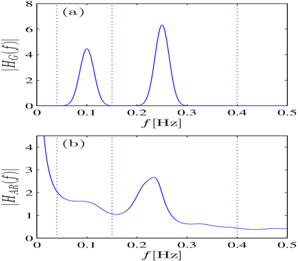
Figure 2: Power spectrum from (a) Equation (3) and (b) Equation (5).

3 Results and discussions

In this work, the power spectrum is considered to obtain the theoretical tachogram and consequently the frequency (Eq. 2) that is used in Equation (2) to build the ECG. We generate $124$ theoretical ECG signals, being $62$ from the Gaussian spectrum and $62$ from the AR spectrum. Then, we obtain their respective tachograms and compare them with $62$ experimental tachograms collected from healthy adults. The experimental protocol consisted of $20$min of monitoring of the heartbeat frequency in resting from patients without sound and visual stimulations in a supine rest position. The heartbeats were recording with a sample rate of $1000$Hz, and $1000$ RR intervals were analysed. The experimental tachograms were filtered to remove ectopic beats and noise effects. We calculate the power spectrum from Gaussian distributions (blue), AR process (red), and experimental data (green), as shown in Figure 3(a). The green dashed lines exhibit the confidence interval of the experimental power spectrum that are calculated from $62$ experimental tachograms.

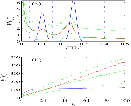
Figure 3: (Colour online) (a) Power spectrum and (b) dentrended fluctuation analysis (DFA) for Gaussian distributions (blue), AR process (red), and experimental data (green). The green dashed lines exhibit the confidence interval of the experimental power spectrum that are calculated from $62$ experimental tachograms.

With regard to Figure 3(a), we see that the power spectrum from AR process has a shape closer the experimental result than the power spectrum from the Gaussian distributions. This way, in order to verify the agreement among the experimental tachogram and the tachograms obtained from theoretical power spectra we have utilised the dentrended fluctuation analysis (DFA) [21, 22]. DFA yields a fluctuation function $F(k)$ as a function of $k$, given by [18]

$$F(k)=\sqrt{\frac{1}{N}\sum_{n=0}^{N-1}[r_{I}(n)-r_{k}(n)]^{2}},$$ (6)

where $N=1000$, $r_{I}(n)=\sum_{l=0}^{n}r(l)$ is the cumulative sum of the $r(n)$, $k$ is the box size that partitions the time interval of the tachogram, and $r_{k}(n)$ is the local trend in each box. DFA is a nonlinear dynamical analysis that have been used for the understanding of biological systems [18]. Moreover, the DFA allows the detection of long-range correlations embedded in a patchy landscape.

Figure 3(b) shows the mean DFAs for $4<k<100$, where linear regressions present slopes equal to $0.1955\pm 0.0150$, $0.7034\pm 0.0686$, and $0.6817\pm 0.2448$ for Gaussian distributions, AR process and experimental data, respectively. The experimental data are collected from $62$ healthy young adults. Each one with length equal to $1000$ heartbeats without trend removal. In general, ectopic beats or noise effects are excluded of time series through filters [23]. As a result, the DFA for the tachogram generated by the experimental data and AR process are in close agreement with each other. Whereas DFA for the Gaussian distributions exhibits a good agreement only for $k<20$.

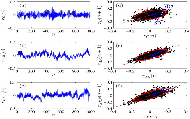
Figure 4: (Colour online) Tachograms generated by (a) the sum of two Gaussian distributions, (b) the AR process, (c) experimental data, and respective Poincaré plots in (d), (e), and (f).

Through the Gaussian power spectrum with phases randomly distributed between $0$ and $2\pi$ we build a ECG and extract the tachogram $r_{G}(n)$ shown in Figure 4(a). A tachogram extracted of ECG generated by the AR spectrum $r_{AR}(n)$ is illustrated in Figure 4(b) and an experimental tachogram $r_{EXP}(n)$ of the healthy adult is in Figure 4(c). In Figures 4(d), 4(e), and 4(f) we calculate the respective Poincaré plots. The Poincaré plot is a visualising technique to analyse RR intervals, where it is computed the standard deviation of points perpendicular to the axis (SD1) and points along (SD2) the axis of line-of-identity. Table 3 exhibits the mean SD1 and SD2 values of the tachograms shown in Figure 4. Comparing the Poincaré plots we see that both SD1 and SD2 for the AR process agree with the experimental results better than the method based on the Gaussian distribution.

In addition, we calculate the $p$-values according to the two-sided Wilcoxon rank sum test [24] of the SD1 and SD2 time series from the simulated and experimental data. This statistical test verifies if two paired time series have the same distribution when the data cannot be assumed to be normally distributed. We find that the $p$-values of SD1 and SD2 are greater than $0.05$ for the AR process, consequently the time series of SD1 and SD2 in the AR process and the experimental data have the same distributions. However, the same does not happen for the Gaussian distributions, where the $p$-values are less than $0.05$.

Table 3: Mean SD1 and SD2 values for the theoretical and experimental tachograms with $p$-values of the Wilcoxon rank sum test.

RR-intervals	$r_{G}(62)$ [A]	$r_{AR}(62)$ [B]	$r_{EXP}(62)$ [C]	$p$-value
SD1 [ms]	$63.9\pm 1.9$	$32.8\pm 10.5$	$38.8\pm 19.6$	$0.0$ [A$\times$C]
				$0.2$ [B$\times$C]
SD2 [ms]	$103.4\pm 2.6$	$82.0\pm 26.2$	$79.0\pm 28.5$	$0.0$ [A$\times$C]
				$0.6$ [B$\times$C]

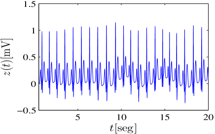
Figure 5: ECG signal generated by means of Equation (2) considering AR process.

All in all, we obtain the tachogram $r(n)$ (discrete-time) by means of the AR process. Then, an interpolation followed by a R-peak detection allows us to determine the signal $r(t)$ (continuous-time). As a result, we calculate $\omega(t)$ and solve the ordinary differential equations to build the ECG signal. We use the fourth order Runge-Kutta method to solve the ordinary differential equations, where we consider a fixed time step $\Delta t=1/f_{s}$ and sampling frequency $f_{s}=256$Hz. Figure 5 shows the ECG signal in the time interval $0\leq t\leq 20$s, where $z(t)$ yields a synthetic ECG with a realistic PQRST morphology according to Figure 1.

4 Conclusions

In conclusion, we have studied a mathematical model given by coupled differential equations that describes electrocardiogram signals and it was proposed by McSharry and collaborators [12]. In the original model, the frequency is calculated from a power spectrum with two Gaussian distributions that incorporates both respiratory sinus arrhythmia and Mayer waves. The use of two Gaussian distributions is in disagreement with our experimental data obtained from healthy adults, due to the fact that the two distributions are not well separated in the power spectrum. This way, we propose to calculate the frequency by means of the AR process. We believe that our model also allows the study of respiratory sinus arrhythmia.

We verify that the power spectrum from AR process has a good agreement with the power spectrum from experimental data. We have also compared the tachograms generated from Gaussian distributions and AR process with the experimental tachogram using DFA and Poincaré plot. As a result, in both DFA and Poincaré plot, the tachogram generated considering the AR process is in closer agreement with experimental data than the two Gaussian. As a consequence, with the tachogram, the frequency is calculated and the ECG signal can be built utilising coupled differential equations with AR process.

We believe that the mathematical model with autoregressive process constitutes an important step toward developing strategies to simulate electrocardiogram signals. We have considered many experimental tachograms from healthy adults to obtain the parameters, this way our simulations allow to obtain and also to do forecast of electrocardiogram signals of individuals in the same situation analysed in this work. We have tested our results using experimental tachograms obtained from $62$ healthy patients without sound and visual stimulations in a supine rest position. In future works, we plan to do the same analyse considering patients with different clinical conditions.

References

- [1] Mohrman DM, Heller LJ. Cardiovascular physiology. New York: McGraw-Hill Education; 2014.
- [2] Curtis H. Biology. New York: Worth; 1989.
- [3] Hall J. Guyton and hall textbook of medical physiology. Philadelphia: Elsevier; 2011.
- [4] Sykes AH. A D Waller and the electrocardiogram. Br Med J 1987; 294:1396-1398.
- [5] Rivera-Ruiz M, Cajavilca C, Varon J. Einthoven’s string galvanometer. Tex Heart Inst J 2008;35:174-178.
- [6] de Gaetano A, Panunzi S, Rinaldi F, Risi A, Sciandrone M. A patient adaptable ECG beat classifier based on neural networks. Appl Math Comput 2009;213:243-249.
- [7] Kudinov AN, Lebedev DY, Tsvetkov VP, Tsvetkov IV, Mathematical model of the multifractal dynamics and analysis of heart rates. Math Models Comput Simul 2015;7:214-221.
- [8] Schenone E, Colin A, Gerbeau J-F. Numerical simulation of electrocardiograms for full cardiac cycles in healthy and pathological conditions. Int J Numer Meth Biomed Engng 2016;32:e02744.
- [9] Van der Pol B. On relaxation oscillations. Philos Mag 1926;7:978-992.
- [10] Gois SRFSM, Savi MA. An analysis of hearth rhythm dynamics using a three-coupled oscillator model. Chaos Solitons Fractals 2009;41:2553-2565.
- [11] Ferreira BB, Savi MA, de Paula AS. Chaos control applied to cardiac rhythms represented by ECG signals. Phys Scripta 2014;89:105203.
- [12] McSharry PE, Clifford GD, Tarassenko L, Smith LA. A dynamical model for generating synthetic electrocardiogram signals. IEEE Trans Biomed Eng 2003;50:289-294.
- [13] Cohen MA, Taylor JA. Short-term cardiovascular oscillations in man: measuring and modelling the physiologies. J Physiol 2002;542:669-683.
- [14] Yasuma F, Hayano J. Why does the heartbeat synchronize with respiratory rhythm? Chest 2004;125:683-690.
- [15] Acharya UR, Joseph KP, Kannathal N, Lim CM, Suri JS. Heart rate variability: a review. Med Bio Eng Comput 2006;44:1031-1051.
- [16] Boardman A, Schlindwein FS, Rocha AP, Leite A. A study on the optimum order of autoregressive models for heart rate variability. Physiol Meas 2002;23:325-336.
- [17] Guzik P, Piskorski J, Krauze T, Schneider R, Wesseling KH, Wykretowicz A, Wysocki H. Correlations between the Poincaré plot and conventional heart rate variability parameters assessed during paced breathing. J Physiol Sci 2007;57:63-71.
- [18] Peng C-K, Buldyrev SV, Havlin S, Simons M, Stanley HE, Goldberger AL. Mosaic Organization of DNA Nucleotides. Phys Rev E 1994;49:1685-1689.
- [19] Oppenheim AV, Schafer RW. Discrete-time signal processing. New Jersey: Pearson Prentice Hall; 2010.
- [20] Proakis JG, Manolakis DG. Digital signal processing. New Jersey: Pearson Prentice Hall; 2007.
- [21] Hu K, Ivanov PCh, Chen Z, Carpena P, Stanley HE. Effect of trends on detrended fluctuation analysis. Phys Rev E 2001;64:011114.
- [22] Chen Z, Ivanov PCh, Hu K, Stanley HE. Effect of nonstationarities on detrended fluctuation analysis. Phys Rev E 2002;65:041107.
- [23] Santos L, Barroso JJ, Macau EEN, Godoy MF. Application of an automatic adaptive filter for Heart Rate Variability analysis. Med Eng Phys 2013;35:1778-1785.
- [24] Wilcoxon F. Individual comparisons by ranking methods. Biometrics Bulletin 1945;1:80-83.