The arrow of time in the collapse of collisionless self-gravitating systems:
non-validity of the Vlasov-Poisson equation during violent relaxation

Abstract

The collapse of a collisionless self-gravitating system, with the fast achievement of a quasi-stationary state, is driven by violent relaxation, with a typical particle interacting with the time-changing collective potential. It is traditionally assumed that this evolution is governed by the Vlasov-Poisson equation, in which case entropy must be conserved. We run N-body simulations of isolated self-gravitating systems, using three simulation codes: NBODY-6 (direct summation without softening), NBODY-2 (direct summation with softening) and GADGET-2 (tree code with softening), for different numbers of particles and initial conditions. At each snapshot, we estimate the Shannon entropy of the distribution function with three different techniques: Kernel, Nearest Neighbor and EnBiD. For all simulation codes and estimators, the entropy evolution converges to the same limit as N increases. During violent relaxation, the entropy has a fast increase followed by damping oscillations, indicating that violent relaxation must be described by a kinetic equation other than the Vlasov-Poisson, even for N as large as that of astronomical structures. This indicates that violent relaxation cannot be described by a time-reversible equation, shedding some light on the so-called “fundamental paradox of stellar dynamics”. The long-term evolution is well described by the orbit-averaged Fokker-Planck model, with Coulomb logarithm values in the expected range $10-12$. By means of NBODY-2, we also study the dependence of the 2-body relaxation time-scale on the softening length. The approach presented in the current work can potentially provide a general method for testing any kinetic equation intended to describe the macroscopic evolution of N-body systems.

1 Introduction

The derivation of reduced dynamical descriptions of large systems composed of many particles is a central issue in Statistical Mechanics. In such systems, the effect of each individual particle is weak, but the collective action of the particle ensemble generates a nontrivial potential field acting on each and every particle. One thus expects that the state of a system with a large number of identical particles is reflected in the statistical behavior of one typical particle in the system. The large scale dynamics is then governed by a set of autonomous equations describing the evolution of the state of this typical particle. In some cases, the effective dynamics emerges in a mathematically rigorous fashion through a scaling limit. One important point to be noted is that the effective macroscopic dynamical equations strongly depend on the particular scaling or regime which is considered: the same (large) system appears differently on different scales. For instance, by considering the same system of Newtonian particles interacting via some well-behaved inter-particle potential, one can arrive at the Boltzmann, Landau, or Vlasov equation, as the effective equation for the “macroscopic” dynamics, depending on the time and space scales, as well as the interaction strength regime considered (Spohn, 2011).

The Boltzmann equation is based on the assumption that particles interactions are short range, instantaneous and involve only two particles at a time (binary collisions). The Vlasov equation is intended to describe the action of smooth collective effects, without considering two-body interactions. The Landau equation is intended to treat binary collisions mediated by the Coulomb interaction. It represents a long-range limit of the Boltzmann equation, and it is based on the idea that the relaxation is produced by the cumulative effects of a large number of weak scatterings (in this way, the Landau equation is also a kind of Fokker-Planck equation), while the “field” particles (the scatterers) are assumed to follow rectilinear trajectories. The Landau equation can also be seen as a long-time correction to the Vlasov equation – see Chavanis (2013) for further discussions relating these equations.

In this context, one of the deepest and most debated questions in Physics since the early development of Statistical Mechanics is the emergence of the arrow of time in the evolution of macroscopic systems and how to reconciliate it with the time-reversible microscopic laws, being them classical, quantum or relativistic (e.g. Ehrenfest & Ehrenfest, 1959; Lebowitz, 1993a, b; Goldstein, 2001). In other words: how to explain, starting from the time-reversible equations of motion for the constituent particles, the irreversibility expressed by the second law of Thermodynamics for the evolution of the system as a whole?

The first to try to solve this problem was L. Boltzmann at the end of the nineteenth century, introducing the equation which now bears his name and the so-called H-theorem, which is intended to prove the entropy increase from mechanical considerations plus statistical assumptions (Brush, 1976). The Boltzmann equation is a particular example of a general class of equations, the transport (or kinetic) equations, which describe the time evolution of the distribution function $f(\vec{r},\vec{v},t)$, the probability for a typical particle to be at position $\vec{r}$ and velocity $\vec{v}$ (Lifshitz & Pitaevskii, 1980).

The basic format of a transport equation is

$$\frac{df}{dt}=\Gamma[f],$$ (1)

where the right-hand side represents the physical process relaxing the system, i.e. driving it to equilibrium, introducing the arrow of time. The main hypothesis behind the use of a transport equation of this form is that the state of the system only depends on its immediately previous state, having no long-term “memory” effects, i.e. that the evolution is Markovian – see Balescu (1975).

In the case of a molecular gas, the process responsible for driving the system to equilibrium is represented by the collisions between molecules. For this reason, $\Gamma[f]$ is traditionally called the collisional term. However, for systems evolving through non-collisional processes, this name can be misleading: relaxation can in principle also be produced by collective, collisionless processes. Henceforth, whenever we refer to the right-hand side of the transport equation, we call it generically the relaxation term, which can be associated to collisional or collisionless relaxation processes.

When deriving the relaxation term, one has to introduce statistical hypotheses related to the type of interactions between the constituent particles. In the case of a neutral molecular gas, as mentioned above, one can assume that the interactions are short-range and that each interaction is a instantaneous binary collision.

Although this discussion has appeared firstly in the study of molecular gases, it applies to any system composed of many interacting particles. In particular, to the process of collapse of self-gravitating systems and the formation of structures in the universe. A self-gravitating system is composed of $N$ gravitationally bound particles moving in the presence of the gravitational potential created by themselves (Spitzer, 1987; Binney & Tremaine, 2008; Saslaw, 1987; Heggie & Hut, 2003). They range from globular clusters, composed of $N\approx 10^{5}$ stars, to galaxies ($N\approx 10^{11}$ stars) and dark matter halos, composed of a giant number of dark matter particles, whose nature is yet unknown. The study of the macroscopic evolution of these systems is of fundamental importance for many reasons, e.g.: they represent the prototype for any long-range interacting system; understanding their macroscopic evolution helps us to theoretically model (beyond the parametrization of the results from numerical simulations) the quasi-stationary state achieved after the relaxation processes and the main functions characterizing this state, namely the density profile and velocity distribution; these functions, besides their intrinsic importance as dynamical diagnostics, are also key ingredients for other analyses such as those of dark matter direct and indirect detection experiments.

The main difference between a self-gravitating system and a neutral molecular gas is that gravity is a long-range interaction, thus invalidating all of the assumptions involved in the derivation of the Boltzmann equation for molecular gases (Prigogine & Severne, 1966; Padmanabhan, 1990). On the other hand, it is still possible to estimate the time-scale for relaxation of a self-gravitating system due to $2$-body processes (long-range “collisions”). A general expression is (see Spitzer, 1987; Binney & Tremaine, 2008)

$$\tau_{col}=k\frac{N}{\ln\Lambda}\cdot\tau_{cr},$$ (2)

where $k\approx 0.1$, $\Lambda=b_{max}/b_{0}$. Here, $b_{max}$ is the maximum impact parameter of the gravitational scatterings, i.e. it plays the role of an effective screening length. The parameter $b_{0}$ is associated to a $90^{\circ}$ scattering angle. – see §6.6 – and $\tau_{cr}$ is the time scale for a typical particle to cross the system, the crossing time, which is also of the same order of the dynamical time scale $\tau_{dyn}=1/\sqrt{\bar{\rho}G}$, where $\bar{\rho}$ is the mean density and $G$ is the gravitational constant.

In the case of a globular cluster, the collisional relaxation time scale is $\tau_{col}\approx 10^{9}$ yr, shorter than its age ($\approx 10^{10}$ yr) and we conclude that the apparent equilibrium of these objects has the $2$-body relaxation as a plausible mechanism, whose relaxation term can be modeled with the Fokker-Planck approximation, which is based on the weak coupling assumption, i.e. that the deflection angle produced by each “collision” is small. Also, it neglects any kind of collective relaxation effect – see §6.2.

For galaxies and dark matter halos, given the large number of particles it is possible to show that the $2$-body relaxation time-scale is $\tau_{col}\gtrsim 10^{17}$ yr, many orders of magnitude larger than their ages, and therefore this process is not a plausible mechanism to explain the apparent (both observationally and in $N$-body simulations) near equilibrium state that can be achieved by these systems. They are thus called collisionless self-gravitating systems and are the main focus of this work (we do not consider any dissipative component such as gas or dust).

The process generally accepted as the driver of a collisionless self-gravitating system to a quasi-stationary state is the interaction of the typical particle with the time-changing collective gravitational potential during the first stages of the collapse of the system (King, 1962; Hénon, 1964; Lynden-Bell, 1967). It is therefore a collective effect, in contrast to $2$-body relaxation. The time-scale for that relaxation process, according to some theoretical arguments (Lynden-Bell, 1967; Kandrup, 1990) and to results from $N$-body simulations, is the dynamical time scale, which is orders of magnitude smaller than the age of any self-gravitating system. This process is called violent relaxation (Lynden-Bell, 1967; Shu, 1978; Madsen, 1987; Shu, 1987; Efthymiopoulos et al., 2007; Bindoni & Secco, 2008; Levin et al., 2014). Considering the N-body problem itself, Gurzadian & Savvidy (1986) have derived, based on the Ergodic theory, another relaxation time-scale associated to collective effects, namely $\tau\propto N^{1/3}\tau_{cr}$, which is still orders of magnitude smaller than Eq. (2).

It is interesting to remember that the relaxation process of a general $N$-body problem is usually related to the presence of stochastic motions that allow the particles to occupy large regions of phase space and the system to forget the initial conditions, the so-called chaotic mixing (Merritt & Valluri, 1996). In fact, $N$-body simulations of galaxy formation have shown evidence of very complex motions in phase space and the fast achievement (in a dynamical time-scale) of a quasi-stationary state – see Merritt (1999) and references therein (see also Kandrup et al. (2003) on the role of chaotic mixing in violent relaxation). This seems to indicate that violent relaxation is a real relaxation process, in the sense that it drives the system irreversibly towards the equilibrium state (see also Kandrup, 1990), even though violent relaxation is known to be incomplete, ending before the achievement of thermodynamical equilibrium, which would be described by a Maxwell-Boltzmann distribution (Merritt, 1999; Kandrup et al., 1993; Efthymiopoulos et al., 2007). Consequently, the system keeps some correlation with the initial conditions. Thus, when we refer to the equilibrium state generated by violent relaxation, we are actually considering this incompletely relaxed, quasi-stationary state, which generally does not correspond to the full thermodynamical equilibrium.

On the other hand, since the $2$-body relaxation of a collisionless self-gravitating system during the early stages of the collapse is by definition negligible, it is usually assumed that the relaxation term associated to violent relaxation is zero. In this case, the system’s evolution is described by Eq. (1) with $\Gamma\left[f\right]=0$:

$$\frac{df}{dt}\equiv\frac{\partial f}{\partial t}+\vec{v}\cdot\frac{\partial f}{\partial\vec{r}}-\frac{\partial\phi}{\partial\vec{r}}\cdot\frac{\partial f}{\partial\vec{v}}=0,$$ (3)

where $\phi(\vec{r},t)$ is the gravitational potential associated to the system as a whole, considered as an external potential for the typical particle: $d\vec{v}/dt=-\nabla\phi$. This equation is generically called the Vlasov equation, which can encompass many different equations, depending on the two-body potential involved. For the specific problem discussed in this work, namely the evolution of self-gravitating systems, the two-body potential is Coulombian, i.e. $\propto 1/r$, and the global potential $\phi$ is self-consistently related to the distribution function $f$ by means of the Poisson equation

$$\nabla^{2}\phi=4\pi G\int d^{3}\vec{v}\,f(\vec{r},\vec{v},t).$$ (4)

Eq. (3), coupled to Eq. (4), is then called the Vlasov-Poisson equation.

Note that, despite the formal similarity of the Vlasov-Poisson equation with the Liouville equation

$$\frac{df^{(N)}}{dt}=0,$$ (5)

where $f^{(N)}(\vec{r}_{1},\vec{v}_{1},...,\vec{r}_{N},\vec{v}_{N},t)$ is the $N$-particle distribution function, in general they represent different descriptions for the system’s evolution. Eq. (5), whose validity is based on mechanical considerations only, describes the evolution of the total system and must be valid under very general conditions (for instance, if the system is subject to external Hamiltonian influences, i.e. if it is described by a time-dependent Hamiltonian).

On the other hand, Eq. (3) refers to the coordinates of one single typical particle while it is also intended to describe the evolution of the system as whole, and thus is clearly based on mechanical plus statistical considerations, what is made explicit in the construction of the BBGKY hierarchy: as pointed out e.g. by Beraldo e Silva et al. (2014), to reduce the full hierarchy of $N$-body evolution equations to an (effective) one-body problem one needs to assume the molecular-chaos hypothesis, i.e. that $f^{(N)}(\vec{r}_{1},\vec{v}_{1},...,\vec{r}_{N},\vec{v}_{N})$ can be written as a $N$-fold product of one-particle distribution functions. Such an assumption is also behind the derivation of other, more general, effective equations.

Additionally, to derive the Vlasov-Poisson from the $N$-body problem, it is usually assumed (see Kandrup, 1998) that the gravitational $N$-body problem converges to the continuous limit for $N\rightarrow\infty$, in some sense. Now define a system as being composed of only one typical particle moving under the influence of the continuous collective potential, this system being thus described by a Hamiltonian, which is time-dependent during violent relaxation. Since Liouville equation is valid even with a time-dependent Hamiltonian, as stressed above, it should be valid in this case, and the Vlasov-Poisson equation is interpreted as the Liouville equation applied to this one-particle system. In this way, the statistical considerations under the Vlasov-Poisson equation are apparently erased and the description becomes purely mechanical. In our opinion, nevertheless, the continuum limit hypothesis only refers to the mean-field approach to the $N$-body problem, which corresponds to the use of self-consistent conditions, in the limit of large $N$, which could depend on many-point correlations. In order to justify the effectiveness of the corresponding one-body, self-consistent, problem, the statistical independence of typical particles is still required. In other words: even if one can consider the Liouville equation applied to any 1-particle phase-space density $f$, associated with the potential generated by the large system, it is not clear from the beginning that such a density $f$ exists for a typical particle representing the system as a whole, unless some justifiable statistical assumption is made.

In addition, it has been already shown (see Valluri & Merritt, 2000; Kandrup & Sideris, 2001; Hemsendorf & Merritt, 2002) that the gravitational $N$-body problem does not converge to the continuous limit for $N\rightarrow\infty$, at least when using Lyapunov exponents as a diagnostic. Note that being a discrete sample with $N$ bodies (stars or dark matter particles), as opposed to the continuous limit, is not a feature of $N$-body simulations only. Most importantly, it is a feature of Nature. Even in the continuous limit, the description of a collisionless self-gravitating system’s evolution in terms of a transport equation is not trivial, specially in the presence of non-integrable potentials generating stochastic orbits – see Binney (1982); Kandrup (1998); Merritt (1999, 2005) for critical discussions relating the presence of stochastic orbits, the $N$-body problem and the Vlasov-Poisson equation.

Furthermore, the main problem in describing the system’s evolution with the Vlasov-Poisson equation is that this equation is time reversible, while it is intended to describe the irreversible evolution driven by violent relaxation. This has been already called the “fundamental paradox of stellar dynamics” (Ogorodnikov, 1965; Ossipkov, 2006).

In fact, this uncomfortable situation can be seen in several works. According to Madsen (1987), “to reach the predicted most probable final state, the system may have to break Liouville’s theorem [Vlasov-Poisson equation]”. Shu (1987) argues that “while Liouville’s theorem [Vlasov-Poisson equation] does apply on a microscopic level, it must necessarily be violated on a macroscopic level if the concept of violent relaxation is to have sensible meaning”. According to Kandrup (1998), “the N-body problem appears to be chaotic on a time scale $∼\tau_{cr}$, but the flow associated with the CBE [Vlasov-Poisson equation] is often integrable or near-integrable in the sense that many or all of the characteristics are regular, i.e., non chaotic. So what do the (often near-integrable) CBE characteristics have to do with the true (chaotic) N-body problem? (…) The correct answer to the question raised above (…) is not completely clear. What does, however, seem apparent from the preceding is that, even for very large N, true $N$-body trajectories could differ significantly from CBE characteristics”. Hemsendorf & Merritt (2002) claim that “if the rate of growth of small perturbations remains substantial even for large N, there would be an important sense in which the CBE does not correctly describe the behavior of $N$-body systems”. Finally, Bindoni & Secco (2008) say that: “any further relaxation of the system should be therefore considered in terms of the coarse-grained phase-space density which, as we have seen, would yield results different from the predictions based on the initial fine-grained phase-space density. This is a worrying aspect of these theories (…). The predictions of the theory, based on the fine-grained density, will then give a wrong result”.

The standard solution to this apparent paradox is to advocate a coarse-grain interpretation to the evolution, according to which the irreversibility is introduced by our inability to follow the phase-space density evolution with absolute precision. In this picture, the transport equation, supposedly the Vlasov-Poisson equation, refers to the fine-grained distribution function, while the irreversible evolution is described by the coarse-grained distribution function. Thus, in this standard picture, it is difficult to see any relation between the assumed transport equation (which refers to the fine-grained distribution function) and the physical phenomenon it is intended to describe. Furthermore, in our view (see also Jaynes, 1965, and §8), this interpretation introduces an undesired subjective element, making the system evolution dependent on observations.

In defense of that standard solution, some authors argue that in the fine-grain level (in the continuous limit), the system develops phase-space structures that are too fine to be followed by any estimator using a finite number of particles, and then in practice we always deal with the coarse-grained distribution function – see e.g. Lynden-Bell (1967). Let us stress once more that real self-gravitating systems always display a finite number of particles, such that one can hardly provide a meaningful interpretation to continuous densities having structures finer than the typical nearest neighbor (phase-space) distance for the given $N$-body system. Globular clusters, for example, which are also expected to violently relax in their early evolution, are composed of $N\approx 10^{6}$ stars, which is the number of particles in the largest $N$-body simulation used in our analysis. In this sense, any coarse graining operating in our results due to the use of a finite $N$ is expected to be the same as that operating in real self-gravitating systems.

In this work, we argue that the apparent paradox disappears once we abandon the assumption of validity of the Vlasov-Poisson equation during violent relaxation. This assumption seems to be due to an oversimplifying treatment of the very singular gravitational (Coulomb) potential and also to a neglect of the proper statistical content of the distribution function regarding the discrete nature of the physical system.

Let us remind that there is no mathematically rigorous proof of the validity of the Vlasov-Poisson equation for self-gravitating systems. In Appendix A we give a summary of recent mathematical results on the derivation of this equation from the $N$-body problem. These suggest that interactions involving impact parameters up to scales that are large compared to the mean neighboring particle distance $\bar{d}$ could prevent the Vlasov-Poisson equation from being the effective macroscopic equation governing the evolution of large gravitational systems. As discussed below, the numerical results obtained here point in the same direction and moreover suggest that violent relaxation does not involve scales much smaller than $\bar{d}$.

Interestingly, studies based on the numerical integration of the Vlasov-Poisson equation sometimes obtain results comparable to those obtained from $N$-body simulations (although frequently simulating situations and scales different from those associated to the violent relaxation process), attributing any difference to $N$-body codes limitations (Yoshikawa et al., 2013; Colombi et al., 2015; Hahn & Angulo, 2016).

As is well known, if the Vlasov-Poisson equation is valid, then the entropy must be conserved (see Tremaine et al., 1986) – see §2. In the present work we use $N$-body simulations, which are described in §3, to estimate the entropy of the system at each snapshot, following its time evolution. The estimators involved in the entropy estimate are presented in § 4. In §5 we show our main results, focusing in the short-term entropy production during violent relaxation. Then, in § 6 we analyze the long-term entropy evolution and its description in terms of a Fokker-Planck equation. Finally we conclude in §7, with further comments in §8.

2 Testing Vlasov-Poisson equation

Going back to the general form of the transport equation, we have

$$\frac{df}{dt}\equiv\frac{\partial f}{\partial t}+\vec{v}\cdot\frac{\partial f}{\partial\vec{r}}-\frac{\partial\phi}{\partial\vec{r}}\cdot\frac{\partial f}{\partial\vec{v}}=\Gamma[f].$$ (6)

As for any good relaxation process, the relaxation term is responsible for entropy increase. In fact, following Tremaine et al. (1986), let

$$S=-\int s[f]\,d^{3}\vec{r}\,d^{3}\vec{v},$$ (7)

where $s[f]$ is some functional of the distribution function $f$. For example, if $s[f]=f\ln f$ then $S$ is the well-known Shannon entropy associated to the distribution $f$. Accordingly,

$$\frac{dS}{dt}=-\int\frac{ds}{df}\frac{\partial f}{\partial t}\,d^{3}\vec{r}\,d^{3}\vec{v}$$ (8)

and using the transport equation (6):

$$\begin{split}\frac{dS}{dt}&=-\int\frac{ds}{df}\left[\Gamma[f]-\vec{v}\cdot\frac{\partial f}{\partial\vec{r}}+\frac{\partial\phi}{\partial\vec{r}}\cdot\frac{\partial f}{\partial\vec{v}}\right]\,d^{3}\vec{r}\,d^{3}\vec{v}\\ &=-\int\frac{ds}{df}\Gamma[f]\,d^{3}\vec{r}\,d^{3}\vec{v}+\\ &+\int\left[\vec{v}\cdot\frac{\partial s}{\partial\vec{r}}-\frac{\partial\phi}{\partial\vec{r}}\cdot\frac{\partial s}{\partial\vec{v}}\right]\,d^{3}\vec{r}\,d^{3}\vec{v}\\ &=-\int\frac{ds}{df}\Gamma[f]\,d^{3}\vec{r}\,d^{3}\vec{v}.\end{split}$$ (9)

In the last passage, we integrate the term $\vec{v}\cdot\partial s/\partial\vec{r}$ firstly in $d^{3}\vec{r}$ and the term $\partial\phi/\partial\vec{r}\cdot\partial s/\partial\vec{v}$ firstly in $d^{3}\vec{v}$, using the fact that $s[f]\rightarrow 0$ for $\vec{r},\vec{v}\rightarrow\infty$.

Thus, if the Vlasov-Poisson equation is valid, i.e. if $\Gamma[f]=0$, then $S$, and particularly the Shannon entropy, is conserved (see Shu, 1978; Tremaine et al., 1986). This is to be expected, since the Vlasov-Poisson equation is time-reversible and reversible processes keep the entropy constant. On the other hand, if the quantity defined by Eq. (7) is not conserved, this is a clear evidence for the non-validity of the Vlasov-Poisson equation and of the emergence of the arrow of time.

The main objective of this work is to test the validity of the Vlasov-Poisson equation during the violent relaxation of collisionless self-gravitating systems. We do this using $N$-body simulations to estimate the entropy of the system at each time, verifying whether it is conserved. While interesting works on the relaxation of self-gravitating systems focus on characterizing the mixing properties of the evolution by means of e.g. calculating Lyapunov exponents or fundamental frequencies (Merritt & Valluri, 1996; Valluri & Merritt, 1998; Kandrup & Sideris, 2001; Kandrup et al., 2003), the key quantity for the relaxation concept, which may be considered to define it, is the entropy. In this sense, this work go straight to the relaxation concept, with no regards to its explanation in terms of mixing.

In what follows, we will set $s[f]=f\ln f$, i.e. we will only consider the Shannon entropy

$$S=-\int f\ln f\,d^{3}\vec{r}\,d^{3}\vec{v}.$$ (10)

3 $N$-body simulations

We use the code NBODY-6 accelerated with a graphics processing unit (GPU) – see Nitadori & Aarseth (2012), which is the result of a long development since its first version NBODY-1 (Aarseth, 1999). It is a direct summation code and the integration is based on the scheme of Ahmad & Cohen (1973) using the forth-order Hermite method (Makino & Aarseth, 1992). The code does not make use of a softening in the Newtonian force law, as commonly done to avoid close encounters (see below). Instead, it implements regularization procedures in order to deal with the possible close encounters, binaries and higher-order objects etc. For a general discussion about these techniques, see Aarseth (2003).

We use NBODY-6 to simulate an isolated self-gravitating system with $N$ particles of equal mass $m$, with an initial Maxwellian velocity distribution with velocity dispersion determined by the initial virial ratio $Q_{0}$, which is defined as the ratio of kinetic energy $T$ and potential energy $W$, $Q=T/|W|$. For our fiducial simulation run, we use $N=10^{5}$ particles with a top-hat initial condition, i.e. a spherically symmetric and spatially homogeneous system, with $Q_{0}=0.5$, the value expected at equilibrium.

We also run simulations with different numbers of particles and different initial conditions: setting $Q_{0}=0.25$ or $Q_{0}=0.6$ (the “cold” and “hot” initial conditions, respectively) for the top-hat configuration. Additionally we run a simulation with the initial condition set to the self-consistent Plummer model which is a stationary state – see §5.1. In all simulation runs, the number of escaping particles, when it occurs, is completely negligible. The maximum allowed energy relative error was set to $5\times 10^{-5}$.

Ideally, a $N$-body simulation code intended to simulate collisionless systems need to run with a (possibly impracticable) large number of particles in order to suppress $2$-body relaxation, at least for the time-scales of interest – see Eq. (2). A widely used strategy is to introduce the softening length parameter $\varepsilon$, modifying the Newtonian gravitational potential to the Plummer-softened one

$$\phi(r)=-\,\frac{G\,m}{\sqrt{r^{2}+\varepsilon^{2}}},$$

and thus avoiding close encounters and suppressing the $2$-body relaxation. In order to study the role of the softening length in the relaxation process, we also run the simulation code NBODY-2 (Aarseth, 2001) that, differently from NBODY-6, does make use of a softening length. This code is also of direct summation type, but the use of the softening length simplifies the treatment of close encounters in comparison to NBODY-6. Unfortunately, there is no parallelized or GPU accelerated version of NBODY-2, what restricts the possibility of using large numbers of particles.

With the aim of testing the universality of our NBODY-2 and NBODY-6 entropy estimation, we also run the publicly available GADGET-2 code (Springel, 2005). GADGET-2 is a hybrid N-body code that combines the traditional evolution of self-gravitating collisionless particles, with the smoothed particle hydrodynamics (SPH) treatment for collisional gas. In our case, we run GADGET-2 using the same initial conditions that were used for NBODY-2 and NBODY-6 simulations, i. e., an isolated set of self-gravitating collisionless particles, within a Newtonian space (without Hubble expansion), and without the presence of any collisional gas. In addition, we run GADGET-2 using its tree configuration, i. e., without using the Fourier techniques to compute long-distance forces.

In order to suppress large-angle scattering during $2$-body encounters, the GADGET-2 code uses the spline-softened gravitational potential:

$$\phi(r)=\frac{G\,m}{h}\,\,W(r/h)\,,$$

where

$$W(u)=\begin{cases}\cfrac{16}{3}u^{2}-\cfrac{48}{5}u^{4}+\cfrac{32}{5}u^{5}-\cfrac{14}{5}\,,&0\leqslant u<\frac{1}{2}\,,\vspace{0.2cm}\\ \cfrac{1}{15\,u}+\cfrac{32}{3}u^{2}-16\,u^{3}\vspace{0.1cm}\\ +\cfrac{48}{5}u^{4}-\cfrac{32}{15}u^{5}-\cfrac{16}{5}\,,&\frac{1}{2}\leqslant u<1\,,\vspace{0.2cm}\\ -\cfrac{1}{u}\,,&1\leqslant u\,,\end{cases}$$

is based on the Monaghan & Lattanzio (1985) SPH modelling, which was constructed guided by the accuracy, smoothness, and computational efficiency criteria. This spline-softened potential is equal to the Newtonian gravitational potential for distances greater than the softening length $h$, unlike the Plummer-softened potential used by NBODY-2, which converges slowly to the Newtonian one for long distances – see Fig. 1. In addition, we will refer to $\varepsilon_{eq}\equiv h/2.8$ as the Plummer-equivalent softening length for a given $h$ set in GADGET-2. With this choice, the minimum of the GADGET-2 and the Plummer-softened gravitational potentials have the same depth at $r=0$, as shown in Fig. 1.

Figure 1: Comparison between the spline-softened GADGET-2, the Plummer-softened and the Newtonian gravitational potentials of a point mass. It was used here $h=1.0$ and $\varepsilon=h/2.8$.

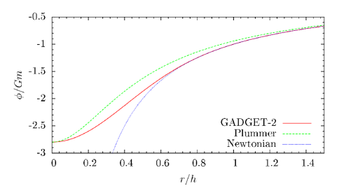
All units adopted here are the same as those used internally and prompted by the simulation code, the Hénon units (see Hénon, 1964), also called $N$-body units, where the gravitational constant is $G=1$, total mass $M=1$, and total energy $E=-1/4$ – see Appendix B. In virial equilibrium, this corresponds to a virial radius $R_{vir}=1$ and rms velocity ${\sqrt{\langle v^{2}\rangle}=\sqrt{2}/2}$, and thus the mean crossing time ${\tau_{cr}=2R_{vir}/\sqrt{\langle v^{2}\rangle}=2\sqrt{2}}$ – see Aarseth (2001) and Appendix B. Importantly, in $N$-body units, positions and velocities are dimensionless quantities and have values of similar magnitudes.

4 Entropy estimators

The entropy given by Eq. (10) is estimated using the data from the $N$-body simulation and translating the integral over phase space into a sum over the $N$ particles of the system (see Joe, 1989; Hall & Morton, 1993; Beirlant et al., 1997). The heuristics behind entropy estimators is as follows: having an estimate $\hat{f}_{i}=\hat{f}(\vec{r}_{i},\vec{v}_{i},t)$ for the distribution function $f$ at the phase space position of each particle $i$, we estimate the entropy at each time as

$$\hat{S}(t)=-\frac{1}{N}\sum_{i=1}^{N}\ln\hat{f}_{i}.$$ (11)

The meaning and adequacy of this estimator becomes clear when we interpret Eq. (10) as the phase space average of $\ln f$. Assuming that the positions $(\vec{r}_{i},\vec{v}_{i})$ of the particles in phase space are independently distributed with distribution $f$, for particular choices of $\hat{f}_{i}$ (e.g., the kernel and nearest-neighbors methods discussed below), it has been shown that this estimator converges in probability to the Shannon entropy given by Eq. (10) in the limit $N\rightarrow\infty$ (Joe, 1989; Hall & Morton, 1993; Beirlant et al., 1997). We remark here that the question whether $\hat{f}_{i}$ is a good estimator for the distribution function $f$ itself, is not explicitly addressed by Joe (1989); Hall & Morton (1993); Beirlant et al. (1997) and related works: instead, the expression in the r.h.s. of (11) is directly proven to be a good entropy estimator for certain technically convenient choices of $\hat{f}_{i}$. Note that assuming the validity of any dynamical equation for one typical particle as the effective equation for the macroscopic dynamics includes the assumption that the many-particle correlations do not participate in the effective dynamics, i.e., different particles typically evolve independently. Hence, seeing the phase space coordinates of particles as independent random variables is part of the hypothesis we are testing, namely, the validity of the Vlasov-Poisson equation. Fig. 2 shows the early (i.e. in a few dynamical time-scales) evolution of this estimation, with the following estimator for the distribution function.

We estimate the entropy of the distribution function $f$ by means of three different methods: the Kernel method, the Nearest Neighbor method (see Silverman, 1986) and the EnBiD method developed by Sharma & Steinmetz (2006). This last method has the advantage that it is fast and metric free, i.e. it does not need to define distances in 6-D phase-space, for which we need to put positions and velocities in the same units, which involves some arbitrary choice – see Eq. (13) and the comments below. On the other hand, mathematical results showing the convergence of Eq. (11) to the real entropy when $\hat{f}_{i}$ is the EnBiD estimator do not exist, as far as we know. Also, in contrast to the Kernel method, the convergence of the Nearest Neighbor is only well-understood at dimension less than 3. Note that Beirlant et al. (1997) only mention the derivation of a rate of convergence for one-dimensional systems, whereas in the case of Kernel estimators explicit bounds are known at any dimension – see Joe (1989); Hall & Morton (1993). For these reasons, the analyses in this work are generally based on the Kernel estimator and in § 5.3 we explain the Nearest Neighbor and EnBiD methods and show the qualitative agreement between the different methods and their apparent convergence for increasing N.

The Kernel method (Silverman, 1986) models the distribution at a specified point $i$ as a sum of “bumps” centered at each one of all the other particles $j$:

$$\hat{f}_{i}=\hat{f}(\vec{r}_{i},\vec{v}_{i},t)=\frac{A}{N}\sum_{j=1}^{N}\frac{1}{h_{j}^{6}}K\left(\frac{D_{ij}}{h_{j}}\right),$$ (12)

where $D_{ij}$ is the phase-space distance (6-D) between particles $i$ and $j$

$$D_{ij}=\sqrt{(\vec{r}_{i}-\vec{r}_{j})^{2}+(\vec{v}_{i}-\vec{v}_{j})^{2}}$$ (13)

(using the dimensionless coordinates and velocities provided by Hénon units – see § 3 and Appendix B) and $K\left(\frac{D_{ij}}{h_{j}}\right)$ is the kernel function, which determines the shape of the bumps. Note that in principle the distance estimator in phase-space $D_{ij}$ would involve coordinates of different units and some metric is necessary to make them compatible (see Ascasibar & Binney, 2005; Sharma & Steinmetz, 2006). One important thing about this metric is that it should produce coordinates with the same covariance along all dimensions, which is approximately provided by the use of Hénon units.

The parameter $h_{j}$, here allowed to vary for different particles (the variable kernel method), is the window width, and it determines the width of the bumps. This parameter introduces a certain degree of arbitrariness, analogous to that associated to the bin definitions of a histogram: it cannot be too small, thus introducing spurious and noisy substructures, nor too large, what would erase important information of the distribution. Choosing this parameters optimally corresponds to improving the convergence rate of the estimator. Here, we take $h_{j}$ to be the phase space distance $D_{jn}$ from particle $j$ to its nearest neighbor (see §5.3), which is a standard choice (see Silverman, 1986, sec. 2.6). Let us emphasize that this does not mean that we only consider the contribution of the nearest neighbor. Instead, the window width just determines the narrowness of the Kernel function at the position of particle $j$, and the contributions (tails) of all particles are important, because the kernels used are heavy-tailed. Note, additionally, that in the current study the radius of the system is approximately one. In particular, $D_{jn}$ is typically $N^{-1/6}$. As in our simulations $N$ ranges between $10^{4}$ and $10^{6}$, in this case $D_{jn}$ lies between circa $0.1$ and $0.21$.

The normalization constant $A$ is defined by the condition

$$A=\frac{1}{\int K(x)\,d^{6}x},$$ (14)

$x$ being a vector in 6-D, and we use the kernel

$$K\left(\frac{D_{ij}}{h_{j}}\right)=\frac{1}{\left(D_{ij}/h_{j}\right)^{8}+1},$$ (15)

which implies $A=8/(\sqrt{2}\pi^{4})\approx 5.807\times 10^{-2}$. Observe that entropy estimators of the form (12), whose kernel $K$ has a “heavy tail” (i.e., decays slowly in space, without destroying integrability) are known to have good convergence properties. See, for instance, Hall & Morton (1993), sec. 3. The particular (heavy-tail) kernel, Eq. (15), was chosen because it has many symmetries in phase space and a simple, explicit normalization constant $A$.

Let us emphasize that there is no need to advocate any coarse-grain interpretation to our estimation of the distribution function besides that present in real systems with finite $N$, since our estimators are not based on phase-space averages of regions containing large numbers of particles. Instead, the distribution function at each phase-space position is estimated directly from the phase-space coordinates of each particle, and the estimators used have been shown to converge to the true entropy in the limit $N\rightarrow\infty$ (Beirlant et al., 1997). Moreover, as shown in § 6, we are able to describe the observed long-term entropy evolution by means of the Fokker-Planck equation. In that case also, there is no need to advocate any extra coarse-grain interpretation.

5 Results: early evolution and violent relaxation

Let us remember that for our fiducial simulation run, we use $N=10^{5}$ particles with a top-hat initial condition, i.e. a spherically symmetric and spatially homogeneous system, with an initial Maxwellian velocity distribution with velocity dispersion determined by the initial virial ratio set to $Q_{0}=0.5$, the value expected at equilibrium.

Fig. 2 shows the initial evolution of the entropy production $\hat{S}(t)-\hat{S}(0)$, as estimated by Eq. (11), with the help of Eqs. (12) to (15). In this and other plots shown below, time is in units of initial mean crossing time $\tau_{cr}=2\sqrt{2}$ – see Appendix B. The uncertainties were calculated as the standard deviation of 50 runs starting with different seeds for the random number generator. We clearly see that the entropy has a significant increase, accompanied by damping oscillations, in the dynamical time-scale, which corresponds to the time-scale during which the violent relaxation process is expected to occur – see § 1.

These oscillations could, naively, be interpreted as a violation of the second law of Thermodynamics, which predicts that the entropy must necessarily increase or be conserved. However, the observed global entropy increase is in accordance to this. What is apparently violated is the so-called H theorem, which predicts a monotonic increase of the H function if the system’s evolution is described by the Boltzmann equation. This apparent violation of the H theorem is, however, a common feature of any system with an appreciable potential energy, as argued by Prigogine & Severne (1966); Jaynes (1971) – see also Romero-Rochin & González-Tovar (1997). As pointed out by those authors, these characteristic oscillations are the consequence of the conversion of kinetic to potential energy and vice-versa, a phenomenon which is known to occur during the collapse of self-gravitating systems. In fact, if we assume as a toy-model that the entropy of these systems has some similarity with that of ideal gases, depending on the volume $V$ as $\propto\ln V$, the behavior seen in Fig. 2 can be associated to the system’s macroscopic oscillations with collapse followed by some diffusive process and the correspondent expansion forming the external halo. Such entropy oscillations are also well-known in presence of memory terms in the effective dynamics.

Figure 2: Entropy production estimation $\hat{S}(t)-\hat{S}(0)$, Eq. (11), for $N=10^{5}$ particles starting with a homogeneous sphere and a Maxwellian velocity distribution, with initial virial ratio $Q_{0}=0.5$, i.e. with the value expected at equilibrium. Time in units of initial mean crossing time $\tau_{cr}=2\sqrt{2}$, the expected time-scale for violent relaxation. Uncertainties were calculated as the standard deviation of 50 runs starting with different seeds for the random number generator. The significant entropy increase contrasts with the entropy conservation predicted by the Vlasov-Poisson equation.

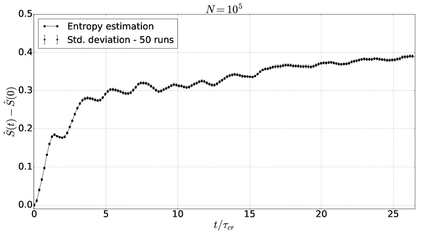
Fig. 2 is the main result of this work. It shows that during violent relaxation of a $N$-body self-gravitating system the entropy has a significant increase, while the prediction of Vlasov-Poisson equation is entropy conservation, what shows that this equation does not seem to be valid during violent relaxation. In what follows, we explore other aspects of the problem, namely the role of the initial conditions, the dependence on the number of particles, the comparison of different N-body simulators and different distribution function estimators and finally the role of the softening length in the codes where it is used. After that we study the long-term evolution of the entropy, investigating all these aspects in relation to the two-body relaxation modelled by means of the orbit-averaged Fokker-Planck equation.

5.1 Changing initial conditions

In this section we study what are the consequences of different initial conditions for the entropy evolution in two different ways. First, we run the same $N$-body simulations as before, with $N=10^{5}$ particles and a top-hat initial spatial distribution with a Maxwellian velocity distribution, but now changing the initial virial ratio $Q_{0}$. Remembering that the expected value at equilibrium is $Q=0.5$ (the value used in the previous analyses), now we set $Q_{0}=0.25$ in one run, which we call “cold” initial condition, and $Q_{0}=0.6$ in the other (“hot”). And second, in another run, we start the simulation with a self-consistent Plummer model (see Aarseth et al., 1974), whose density profile is given by

$$\rho(r)=\frac{3M}{4\pi a^{3}}\frac{1}{\left[1+\left(r/a\right)^{2}\right]^{5/2}},$$

where $M$ is total mass and $a$ is a scale factor. In this way, this simulation run already starts with a steady-state, for which we would expect no entropy increase.

Fig. 3 shows the early entropy evolution for these configurations. We see that all three curves with a top-hat initial density profile and varying $Q_{0}$ show the same qualitative behaviour: a high entropy increase followed by damping oscillations, in the dynamical time-scale. On the other hand, this early entropy increase is significantly smaller (virtually negligible) for the initial Plummer model. In Fig. 3, time is again in units of the initial mean crossing time. Note that this quantity depends on $Q$ (see Appendix B), which also changes in time, oscillating around and converging to the value expected at equilibrium, $Q=0.5$. For $Q_{0}=0.25$ and $Q_{0}=0.6$ the initial mean crossing time would be $\tau_{cr}\approx 7.35$ and $\tau_{cr}\approx 1.85$, respectively. However, in order to avoid confusion, we normalize all curves by the same constant value $\tau_{cr}(Q=0.5)=2\sqrt{2}$. If we had normalized by the respective $\tau_{cr}$ values, the blue (cold) curve would be slightly compressed to the left and the red (hot) curve would be slightly stretched out to the right.

Figure 3: Entropy estimation for $N=10^{5}$ particles and different initial conditions. Blue triangles: initial virial ratio $Q_{0}=0.25$ (“cold” initial condition). Red squares: $Q_{0}=0.6$ (“hot” initial condition). Black dots: the same as in Fig. 2, the case $Q_{0}=0.5$ (the value expected at equilibrium). Black stars: initial self-consistent Plummer model, which is a steady-state. Time in units of initial mean crossing time $\tau_{cr}=2\sqrt{2}$, the time-scale expected for violent relaxation. All these curves are consistent with the expectation that the farther from the equilibrium, the larger the entropy production.

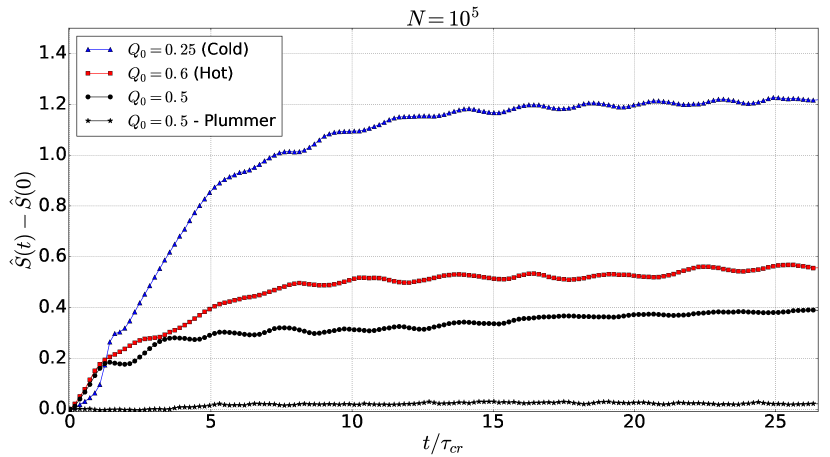
The most striking feature of this plot is the fact that when we start with initial conditions farther from equilibrium the entropy increase is higher, as we would expect based on the second law of Thermodynamics. For the simulation starting with the self-consistent Plummer model, the entropy production is almost zero. Therefore, the large entropy increase observed in the other curves probably cannot be attributed to any artificial numerical effect. Instead, as in the general idea of the entropy increase in any macroscopic system, it is the consequence of the choice of a particular initial state, very unlikely in comparison to the near-equilibrium state.

5.2 Dependence on the number of particles

The distribution function estimation is expected to represent the true distribution function and, for significantly large $N$, the distribution function of a collisionless system. One concern then is whether the number of particles used is enough for achieving convergence to this limit.

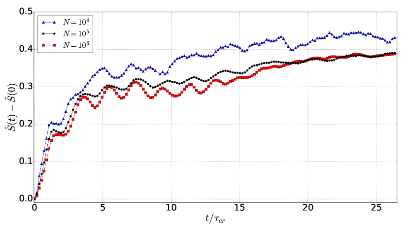
Fig. 4 shows the early entropy evolution for different numbers of particles (blue triangles for $N=10^{4}$, black dots for $N=10^{5}$ and red squares for $N=10^{6}$). We see that the three curves have the same qualitative behaviour: a fast entropy increase, followed by damping oscillations. For $N=10^{4}$, we still have significant noise deforming the oscillatory pattern, while for $N=10^{5}$ and $N=10^{6}$ the curves are smoother. Also, the curves for $N=10^{5}$ and $N=10^{6}$ are very similar and achieve the same value at $t\approx 75$, what seems to indicate the convergence for this early evolution. This convergence is also important because it indicates that the high entropy increase during violent relaxation is not due to two-body relaxation associated to the use of a finite number of particles.

Figure 4: Entropy estimation for different numbers of particles as a function of time. Blue triangles for $N=10^{4}$, black dots for $N=10^{5}$ and red squares for $N=10^{6}$. The similarity between the curves for $N=10^{5}$ and $N=10^{6}$ suggests the convergence for significantly large $N$.

5.3 Comparison of distribution function estimators

The second method we use to estimate the distribution function $f(\vec{r},\vec{v},t)$ is the Nearest Neighbor method (see Silverman, 1986), which is based on the following idea: sitting on particle $i$, we use Eq. (13) to calculate the (6-D) phase space distance $D_{in}$ to particle $n$, its nearest neighbor, i.e. the smallest of the distances to all the other particles $j$, Eq. (13).

This distance is used to define a hyper-sphere of volume $\propto D_{in}^{6}$ centered on particle $i$. The estimation of the distribution function at the phase-space position of particle $i$ is then

$$\hat{f}(\vec{r}_{i},\vec{v}_{i},t)=\frac{1}{D_{in}^{6}},$$ (16)

i.e., it is the number of particles inside the sphere divided by its volume. In principle, this estimation must be normalized, but we use it just to estimate the entropy production $S(t)-S(0)$, for which additive constants, i.e. multiplicative factors in $f$, cancel out. Note that, differently from the Kernel method, Eq. (12), the Nearest Neighbor estimation does not involve a sum over particles. Instead, it only considers the distance to the nearest neighbor, thus being more prone, at least in principle, to larger Poisson errors.

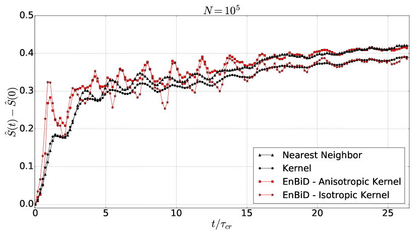
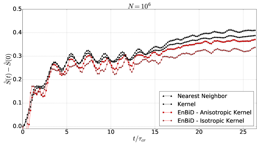
Figs. 5 and 6 compare the early entropy evolution obtained with the different estimator methods, for $N=10^{5}$ and $N=10^{6}$ respectively. Results obtained with Nearest Neighbor method are represented by black triangles. We see that for $N=10^{5}$, this method is already very close to the Kernel method estimation (black dots), although showing larger amplitude oscillations. For $N=10^{6}$, Fig. 6, the differences are smaller and the oscillation amplitudes are very close to those obtained with the Kernel method.

Figure 5: Entropy estimation for $N=10^{5}$ with different methods. Black dots (triangles) show the entropy estimation obtained with Kernel (Nearest Neighbor) method, Eqs. (12) and (16). Red squares (stars) represent the entropy evolution obtained with EnBiD method with anisotropic (isotropic) kernel smoothing. Despite some differences, mainly the higher initial entropy production obtained with EnBiD in comparison to the other methods, the overall behavior of the estimation does not change for different estimators: entropy increases accompanied by damping oscillations.

Figure 6: Same as Fig. 5 but now for $N=10^{6}$ particles. The larger initial entropy production obtained with EnBiD in comparison to the other methods is not present anymore and the oscillation amplitudes of all methods are closer. Qualitative changes of EnBiD from $N=10^{5}$ to $N=10^{6}$ are larger than for the other methods, suggesting a faster convergence of Nearest Neighbor and Kernel methods. The similarity of all curves also suggests convergence for significantly large $N$.

The third distribution function estimator method we use is EnBiD (Sharma & Steinmetz, 2006) which is based on the general idea of binary space partitioning tree, and consists of three steps: first the phase space is tessellated into mutually disjoint hyper-cubes containing one particle each. Here, the phase-space density could already be estimated as $1/V_{i}$, where $V_{i}$ is the volume of hyper-cube $i$, similarly to the Nearest Neighbor method. Then, boundary corrections are applied to consider the arbitrary shape of the volume with the data. Finally, in order to reduce noise, that first density estimation is smoothed by a number of different techniques, mainly the Kernel method. Also, different kernels can be chosen. In this smoothing procedure, EnBiD sums the contribution of a fixed number of neighbors. Note that this is different from what we do in the Kernel estimator, where we sum over all systems’s particles – see § 4. As a generalization, EnBiD also allows the use of Anisotropic Kernels, what can improve the estimation in regions with large density variations, such as the borders of the system – see Maciejewski et al. (2009).

EnBiD has been shown to accurately recover the distribution function used as input – Sharma & Steinmetz (2006); Maciejewski et al. (2009). Here we use EnBiD method with the Epanechnikov Kernel smoothing, taking into account the contribution of 25 neighbors. For comparison, we also use EnBiD with the anisotropic kernel option. In Figs. 5 and 6, the EnBiD estimates are represented by red squares and stars, for the Anisotropic and Isotropic kernels, respectively. For $N=10^{5}$, we see important deviations in respect to the other two methods, mainly in the initial entropy increase and in the oscillation amplitudes, although the differences being smaller for the Anisotropic version, which we consider to be more accurate. For $N=10^{6}$, the EnBiD estimators, mainly with the Anisotropic kernel, are very close to what is obtained with the Nearest Neighbor and Kernel methods: that high discrepancy in the initial entropy production is not present and the oscillation amplitudes are smaller and similar to those of the other methods. It is interesting to note that the qualitative changes in EnBiD estimate from $N=10^{5}$ to $N=10^{6}$ are larger than that of the Nearest Neighbor and Kernel methods, suggesting a faster convergence of the latters.

The important point here is that all the different methods show the same qualitative behavior for the entropy evolution: a fast monotonic increase up to the dynamical time-scale, followed by an increase with damping oscillations up to, at least, $t/\tau_{cr}\approx 25$. The similarity and smoothness of the curves obtained with different methods indicate that the features observed really represent the behaviour of the entropy during the evolution of the simulated system, and are not spurious effects associated to a particular method. It is interesting to note the similarity of all the methods for $N=10^{6}$. Both the Kernel and the Nearest Neighbor estimators are known to converge, independently of each other, to the same value (namely, the entropy of the considered distribution) for sufficiently large $N$, and the same is expected for EnBiD. Thus, this agreement suggests that this convergence has already been achieved with $N=10^{6}$ particles.

5.4 Comparison of N-body simulators and the role of the softening length

As mentioned in § 3, we also run simulations with the code NBODY-2, which makes use of a softening length in order to avoid close encounters and suppress $2$-body relaxation. Varying that parameter allows us to study the characteristic scales for different relaxation processes. Some particularly important scales in this respect are the system’s size $R\approx 1$ and the mean neighboring particle distance $\bar{d}=R/N^{1/3}$.

Fig. 7 shows the early evolution of the entropy for a simulation with $N=10^{5}$ and the fiducial initial conditions, i.e. a top-hat with Maxwell velocity distribution and initial virial ratio $Q_{0}=0.5$, for different values of the NBODY-2 softening length $\varepsilon$. Black stars represent the entropy evolution obtained with NBODY-6, i.e. without any softening ($\varepsilon=0$). We firstly note the similarity of this curve with the entropy evolution obtained with NBODY-2 for the smallest softening length used $\varepsilon=10^{-3}$ (red dots).

It is possible to see that the initial entropy increase is essentially the same for all runs with $\varepsilon\leq 0.1$, suggesting that violent relaxation do not involve scales much smaller than the mean neighboring particle distance $\bar{d}\approx R/N^{1/3}\approx 0.02$. On the other hand, for $\varepsilon=0.5$ and $\varepsilon=1.0$, we observe an important suppression in the early entropy production, suggesting that the violent relaxation process involves scales larger than $\bar{d}$. We notice that this is in accordance with recent mathematical results on effective dynamical equations for large Newtonian systems, i.e. that interactions involving scales around $\bar{d}$ could prevent Vlasov-Poisson equation to be valid – see Appendix A.

The delayed entropy increase for these large values of $\varepsilon$ can be interpreted as follows: with such high values of $\varepsilon$, the system starts evolving almost as if it was composed of non-interacting particles, for which we would expect the entropy to be constant or to evolve slowly due to phase-mixing finite-$N$ coarse graining. However, once the system expands, the typical distance between particles increases, “turning on” the interactions between particles with distances larger than $\varepsilon$, thus increasing the entropy production rate.

Figure 7: Entropy estimation (Kernel method) for $N=10^{5}$ particles obtained with NBODY-2 for different values of softening length $\varepsilon$. Entropy production is suppressed for $\varepsilon$ values considerably larger than $\bar{d}\approx R/N^{1/3}\approx 0.02$. Black stars represent the entropy obtained with NBODY-6 (same as in Fig. 2), i.e. with $\varepsilon=0$. Also shown the entropy obtained with GADGET-2 (blue open triangles) for a softening length $h=2.8\times 10^{-2}$, i.e. with a Plummer-equivalent $\varepsilon_{eq}=10^{-2}$, whose evolution is very similar to that of NBODY-2 with same $\varepsilon$ (blue dots).

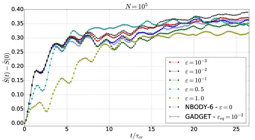
We also simulate the evolution of one halo with the tree code GADGET-2, starting with exactly the same initial conditions as those of the previous simulations, and with a softening length $h=2.8\times 10^{-2}$, i.e. with a Plummer-equivalent softening length $\varepsilon_{eq}=10^{-2}$ – see §3. The entropy evolution is shown as the blue open triangles in Fig. 7 and we see that it is very similar to that obtained with NBODY-2 and the same value of the softening length (blue dots). Since these codes are based on very different integration techniques, this weakens the possibility of the entropy evolution observed being due to an artificial numerical relaxation, unless it is present in exactly the same way in both codes.

6 Long-term evolution and two-body relaxation

Taking into account the collisional relaxation time scale, Eq. (2), in the limit $N\rightarrow\infty$ the system becomes collisionless, i.e. the $2$-body relaxation is expected to be negligible in this limit. The study of this limit is the main goal of this work, as discussed in the previous section. However, in N-body simulations we necessarily deal with a limited number of particles, and some $2$-body relaxation is always present. In this section, we model the effects of $2$-body relaxation by means of the orbit-averaged Fokker-Planck equation, assuming that the potential is static and that the distribution function is a function of energy only. Thus, this approach applies to the long-term evolution, after violent relaxation. The terms involved in the Fokker-Planck relaxation term are estimated with the Agama library (Vasiliev, 2017 - submitted), as explained below.

6.1 Entropy production of a general process

Given the entropy definition Eq. (10), we have, according to Eq. (9),

$$\frac{dS}{dt}=-\int(1+\ln f)\Gamma[f]\,d^{3}\vec{r}\,d^{3}\vec{v},$$ (17)

which we can estimate as

$$\widehat{\frac{dS}{dt}}=-\frac{1}{N}\sum_{i=1}^{N}\frac{(1+\ln\hat{f}_{i})}{\hat{f}_{i}}\Gamma[\hat{f}_{i}].$$ (18)

Thus, the theoretical prediction for the entropy produced by any model through the relaxation term $\Gamma[f]$ can be estimated with the simulation data, then integrating $\widehat{dS/dt}$ as

$$\hat{S}(t+\Delta t)=\hat{S}(t)+a\cdot\widehat{\frac{dS}{dt}}(t)\Delta t$$ (19)

and fitting to the simulation data with 2 free parameters, $S_{0}=S(0)$ and $a$. This can be compared to the entropy production obtained with the same data, Eq. (11), configuring a general method to test any theoretical transport equation, in particular the Fokker-Planck equation.

6.2 Fokker-Planck relaxation term

The Fokker-Planck relaxation term is used below to estimate the $2$-body relaxation contribution to entropy production. This model considers the relaxation of the system as a result of cumulative effects of many $2$-body weak encounters, with the energy change and deflection angle in each encounter being small, neglecting any possible collective relaxation effect, i.e. assuming that encounters are independent on each other. Following standard procedures (Spitzer, 1987; Binney & Tremaine, 2008; Heggie & Hut, 2003), we only consider diffusion in the velocity field. In the local approximation, the diffusion coefficients are considered to depend only on the velocity of the test particle, but not on its position, which is valid for systems with a constant potential. For more realistic systems, in which the potential does have a spatial dependence, we resort to the orbit-averaged Fokker-Planck equation, in which case the diffusion coefficients are averaged over the volume $V$ accessible to the test particle. For a spherically symmetric static potential and assuming that the distribution function depends only on energy, the orbit-averaged Fokker-Planck relaxation term is given by

$$\Gamma[f]_{FP}=\frac{1}{g(E)}\left\{-\frac{d}{dE}\left[f(E)g(E)\langle\Delta E\rangle_{V}\right]+\right.\\ \left.+\frac{1}{2}\frac{d^{2}}{dE^{2}}\left[f(E)g(E)\langle(\Delta E)^{2}\rangle_{V}\right]\right\},$$ (20)

where $g(E)$ is the density of states:

$$g(E)=16\pi^{2}\int_{0}^{r_{m}(E)}drr^{2}v,$$ (21)

with $v=\sqrt{2[E-\phi(r)]}$. The diffusion coefficients $\langle\Delta E\rangle$ and $\langle(\Delta E)^{2}\rangle$ are given by

$$\langle\Delta E\rangle=\gamma(I_{0}-I_{1/2}),$$ (22)

$$\langle(\Delta E)^{2}\rangle=\frac{2}{3}\gamma v^{2}(I_{0}+I_{3/2}),$$ (23)

where $\gamma=16\pi^{2}G^{2}m\ln\Lambda$ and

$$I_{0}(E)=\int_{E}^{0}f(E^{\prime})dE^{\prime}=\int_{v}^{\infty}f(r,v^{\prime})v^{\prime}dv^{\prime},$$ (24)

$$\begin{split}I_{n/2}(E,r)&=\int_{\phi(r)}^{E}\left(\frac{E^{\prime}-\phi(r^{\prime})}{E-\phi(r)}\right)^{n/2}f(E^{\prime})dE^{\prime}\\ &=v\int_{0}^{v}\left(\frac{v^{\prime}}{v}\right)^{n+1}f(r,v^{\prime})dv^{\prime}.\end{split}$$ (25)

Finally, the orbit-average operation is defined as

$$\langle...\rangle_{V}=\frac{16\pi^{2}}{g(E)}\int_{0}^{r_{m}(E)}drr^{2}v\langle...\rangle$$ (26)

– see Vasiliev (2015) for similar expressions. After some algebra, we have

$$\Gamma[f]_{FP}=\gamma\Bigg{\{}\Big{[}\langle I_{0}(E)\rangle_{V}+\langle I_{1/2}(E,r)\rangle_{V}\Big{]}\frac{df}{dE}+\Bigg{.}\\ +\frac{1}{3}\Big{[}\langle v^{2}I_{0}(E)\rangle_{V}+\langle v^{2}I_{3/2}(E,r)\rangle_{V}\Big{]}\frac{d^{2}f}{dE^{2}}+f^{2}(E)\Bigg{.}\Bigg{\}}$$ (27)

We estimate all quantities involved in the orbit-averaged Fokker-Planck relaxation term using the Agama library (Vasiliev, 2017 - submitted), which works in the following steps: for the $N-$body sample at a given snapshot, the library determines a smooth global potential $\phi(r)$ and the density of states $g(E)$, Eq. (21). Given the sample energy distribution $N(E)=f(E)g(E)$ the code calculates smooth functions $f(E)$, $df/dE$ and $d^{2}f/dE^{2}$. The Agama library also provides accurate estimates for the orbit-average of the integrals involved in the calculation of the diffusion coefficients, Eqs. (22)-(25).

Substituting these expressions into Eq. (27), we estimate at each snapshot the contribution of the Fokker-Planck relaxation term to the entropy increase, Eq. (18). This is then integrated with Eq. (19) and fit to the simulation data, with the free parameter $a$ being associated to the value of the Coulomb logarithm $\ln\Lambda$.

Note that, in principle, it is possible to estimate all quantities involved in Eq. (27) with the same kind of estimators used here for the entropy. For example, it is possible to estimate the orbit-averaged diffusion coefficients and, given the estimator for $f(r,v)$, Eq. (12), to calculate $\partial\hat{f}/\partial v$ and $\partial^{2}\hat{f}/\partial v^{2}$. However, when trying this we observed that, although our estimates for the diffusion coefficients seem very accurate, being essentially identical to what we get with the Agama library, our estimates for the derivatives of $f$ are noisy, producing unsatisfactory results. Note also that, even though we are able to get expressions for terms like $\partial\hat{f}/\partial v$, i.e. for the derivative of the estimator, in reality what we need are terms like $\widehat{\partial f/\partial v}$, i.e. the estimator of the derivative. In other words, it is not clear if the estimators commute with the derivatives, and a detailed study of these properties is out of the scope of this work. In future works, it would be interesting to better understand these operators and how to accurately estimate these derivatives, opening the possibility of testing any theoretical transport equation.

6.3 Main results on two-body relaxation

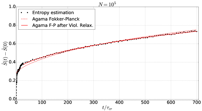
Fig. 8 shows the entropy production estimation ${\hat{S}(t)-\hat{S}(0)}$ in the long-term evolution ($t/\tau_{cr}$ up to $700$) for the fiducial simulation. After the fast increase at early times, as shown in Fig. 2, the entropy growth becomes slower and almost linear. The dashed curve shows the fit of the Fokker-Planck model when we consider all the data points. Since in the early evolution the hypotheses behind the Fokker-Planck model, namely a static potential and $f=f(E)$ are not valid, it is not surprising that the model cannot describe the data in this regime. On the other hand, if we restrict the fit to later times, say for $t/\tau_{cr}\gtrsim 26.5$, we see an excellent agreement with data, as shown by the solid line. Thus this long-term evolution can clearly be attributed to $2$-body relaxation. Note that the smooth, almost linear behaviour of the Fokker-Planck prediction is not put by hand, but it is a consequence of the non-trivial combination of several terms in Eq. (27).

Figure 8: Entropy estimation for $N=10^{5}$ particles (dots) and Fokker-Planck (F-P) prediction estimated by Agama (curves). Note the difference in the range of the x-axis compared to Fig. 2. Dashed line: fit of F-P equation, Eqs. (27) and (18), taking into account all the data points. The high entropy production during violent relaxation at early stages cannot be described by $2$-body relaxation as modeled by F-P equation. Solid line: fit of the same model, but taking into account just data points for $t/\tau_{cr}>26.5$. The model can fit the entropy evolution in this regime.

6.4 Changing initial conditions

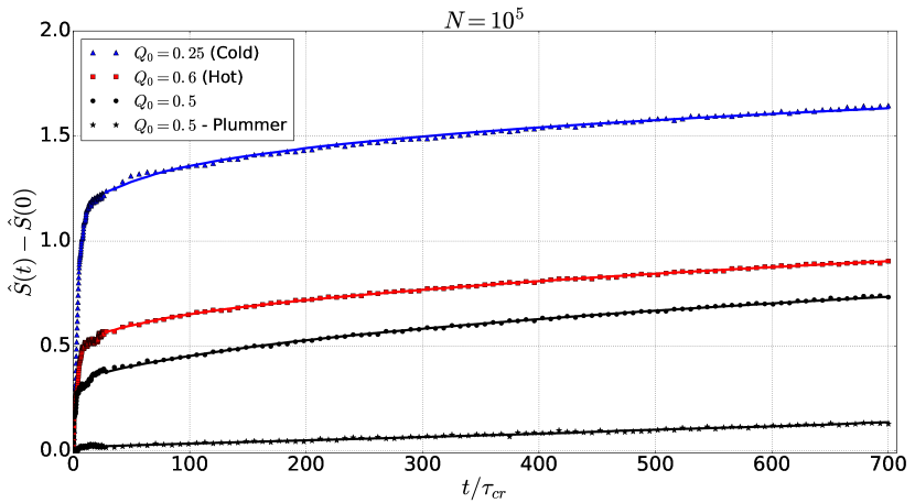
Fig. 9 shows the long-term entropy evolution for the simulations with different initial conditions discussed in § 5.1, namely: top-hat with $Q_{0}=0.25$ (blue triangles), $Q_{0}=0.5$ (black dots) and $Q_{0}=0.6$ (red squares); and also starting with a Plummer model (black stars). As in the fiducial case, the Fokker-Planck model (continuous lines) can reproduce the almost linear entropy increase for $t/\tau_{cr}\gtrsim 26.5$, but not for early times. While the entropy increase at early times depends crucially on the initial conditions, it is basically the same for the long-term evolution (same slope of $\hat{S}(t)$). In other words, collisional relaxation seems to depend just on $N$, but not on the initial conditions, while violent relaxation strongly depends on the initial conditions. Here again we have time normalized by $\tau_{cr}=2\sqrt{2}$ in all curves (normalizing by the respective initial values of $\tau_{cr}$ would give the false impression that the long-term relaxation rate, i.e. the slope of $\hat{S}(t)$, is different for the different initial conditions.)

Figure 9: Long-term entropy evolution for different initial conditions: top-hat with $Q_{0}=0.25$ (blue triangles), $Q_{0}=0.5$ (black dots) and $Q_{0}=0.6$ (red squares); and also an initial Plummer model (black stars) – see Fig. 3. The orbit-averaged Fokker-Planck equation (curves) can describe the long-term entropy evolution (for $t/\tau_{cr}\gtrsim 26.5$), but not the early evolution driven by violent relaxation. Two-body relaxation rate seems to be insensitive to initial conditions.

6.5 Comparison of distribution function estimators

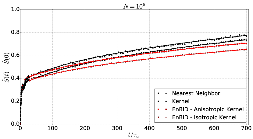
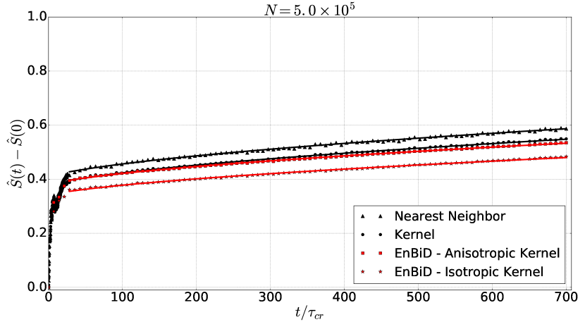
Here we compare the long-term entropy evolution obtained with the three different distribution function estimator methods, as explained in § 5.3. Figs. 10 and 11 show the results for $N=10^{5}$ and $N=5\times 10^{5}$, respectively. In these figures, we can see that the long-term evolution obtained with all methods are very similar already for $N=10^{5}$ particles, with only a slightly smaller slope for the EnBiD estimate. For $N=5\times 10^{5}$, Fig.11, the agreement of the methods is even better, mainly the Kernel and EnBiD with anisotropic smoothing kernel methods. This indicates again that the estimates, which involve different techniques from each other, are capturing real physical effects, and are not produced by numerical features.

Figure 10: Same as Fig. 5, but now showing the long-term evolution of the entropy. We see that all estimators provide the same behavior for the entropy, which increases almost linearly in the $2$-body relaxation time-scale. Continuous curves represent the orbit-averaged Fokker-Planck fit, estimated with Agama library.

Figure 11: Same as Fig. 10, but now for $N=5\times 10^{5}$ particles. The agreement between Kernel method and EnBiD with anisotropic smoothing kernel is almost perfect.

6.6 Dependence on the number of particles

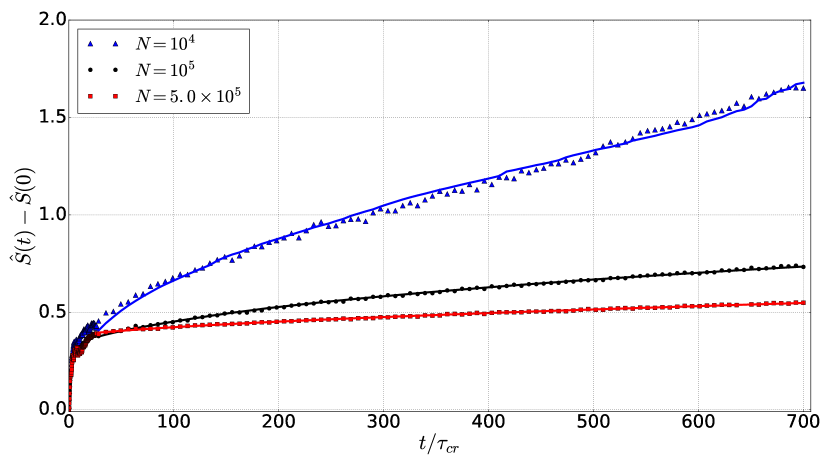
In Fig. 12 we compare the long-term entropy evolution for three different numbers of particles: $N=10^{4}$ (blue triangles), $N=10^{5}$ (black dots) and $N=5\times 10^{5}$ (red squares), as well as the fit of the orbit-averaged Fokker-Planck equation for $t/\tau_{cr}\gtrsim 26.5$. We see that the prediction for $N=10^{4}$ is a little bit noisy. In principle, this can be attributed to two causes: shot noise due to a relatively small number of particles or non-validity of some hypotheses on which our Fokker-Planck model is based. In §6.7 we present arguments in favour of this second option. More specifically, it seems that when $N$ is small we still have a substantial number of almost close encounters ($b\gtrsim b_{0}$), producing scattering angles $\lesssim 90^{\circ}$, which can be enough to violate the weak coupling assumption on the basis of the Fokker-Planck treatment – see Binney & Tremaine (2008), sec. 7.4.4.. However, again we see that in general the Fokker-Planck equation is able to explain the long-term entropy evolution. Taking into account the estimate of the $2$-body relaxation time-scale, Eq. (2), the fact that the slope of $S(t)$ is larger for decreasing number of particles shows that the $2$-body relaxation is in fact more effective for a smaller number of particles, in agreement with the theoretical expectation: in the limit $N\rightarrow\infty$ we would have a collisionless system and thus the slope of $S(t)$ predicted by the Fokker-Planck equation would be zero.

Figure 12: Entropy estimation for $N=10^{4}$ (blue triangles), $N=10^{5}$ (black dots) and $N=5\times 10^{5}$ (red squares). Similarly to Fig. 8 but now comparing different number of particles. The entropy increase during violent relaxation is similarly high for the three data sets. However, for the long-term evolution, during which we expect the $2$-body relaxation to be significant, the slope of $S(t)$ is larger for a smaller number of particles $N$, in agreement with the theoretical expectation that $2$-body relaxation rate is larger for smaller $N$ – see Eq. (2).

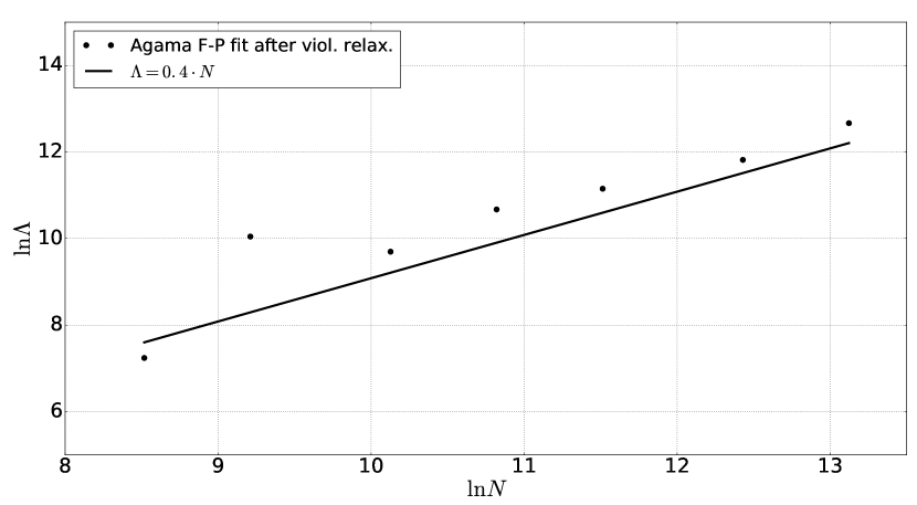
With this long-term entropy evolution for different numbers of particles, we can also study the $N$-dependence of the $2$-body relaxation time-scale, Eq. (2). More specifically, we study the $N$-dependence of the Coulomb logarithm $\ln\Lambda$ obtained with the fit to this long-term evolution. This is represented by the black dots in Fig. 13. From the theoretical point of view, the Coulomb logarithm is given by ${\ln\Lambda=\ln b_{max}/b_{0}}$, where $b_{max}$ is usually assumed to be of order of the system’s size (although some authors support the idea that $b_{max}$ should be equal to the mean interparticle distance, i.e. $b_{max}\propto N^{-1/3}$ – see Chandrasekhar & von Neumann (1942); Kandrup (1980); Farouki & Salpeter (1982); Smith (1992); Farouki & Salpeter (1994); Theis (1998)). In what follows, we set ${b_{max}=R_{hm}}$, the half-mass radius (see Spitzer, 1987). The impact parameter associated to a $90^{\circ}$ scatter is given by:

$$b_{0}=2\frac{Gm}{V^{2}},$$ (28)

where $V$ is the relative velocity between the test and field particles (here again assumed to have equal mass $m$).

The virial radius $R_{vir}$ is defined by (see Appendix B)

$$\langle v^{2}\rangle=\frac{GM}{2R_{vir}}.$$

Substituting in Eq. (28) we obtain

$$\frac{R_{vir}}{b_{0}}=\frac{N}{2}\frac{V^{2}}{2\langle v^{2}\rangle}.$$ (29)

Assuming a Plummer density profile, the half-mass radius is given by $R_{hm}\approx 0.8R_{vir}$ and with $\langle V^{2}\rangle=2\langle v^{2}\rangle$ and assuming the system is virialized (see Appendix B), we finally have

$$\Lambda=\frac{R_{hm}}{b_{0}}\approx 0.4N.$$ (30)

In Fig. 13, this relation is shown as the black straight line. We see that despite some discrepancy for small $N$, the data points show a reasonable agreement with Eq. (30).

Figure 13: Coulomb logarithm obtained fitting Agama modelling of orbit-averaged Fokker-Planck equation to the long-term entropy evolution for different numbers of particles (black dots). We can see a reasonable agreement with the theoretical expression $\ln\Lambda=0.4N$ shown as the black straight line.

6.7 Comparison of different N-body codes and the role of the softening length

Similarly to § 5.4, we now compare the long-term entropy evolution obtained with the three different N-body simulation codes used (NBODY-6, NBODY-2 and GADGET-2) with different values of the softening length, when it applies. Fig. 14 shows the long-term entropy evolution and the fit of the Fokker-Planck model for different values of $\varepsilon$ obtained with NBODY-2, now fixing $N=10^{4}$. The stars and the black dashed line represent the case obtained with NBODY-6, i.e. without softening length. Firstly, we can see that for ${\varepsilon=10^{-4}\approx R/N}\approx b_{0}$ (see Eq. (30)), the entropy evolution is very similar to that without softening length, i.e. encounters with impact parameter $b\lesssim b_{0}$, i.e. close encounters, do not seem to contribute significantly to the relaxation, confirming earlier results from Farouki & Salpeter (1982).

On the other hand, we clearly see that larger values of the softening length increasingly suppress the $2$-body relaxation, decreasing the slope of $\hat{S}(t)$, even for $\varepsilon>\bar{d}=R/N^{1/3}\approx 0.05$. This indicates that scatterings involving distances $>\bar{d}$ seem to be important for the $2$-body relaxation, an indication in favor of ${b_{max}\approx R}$, in contrast to $b_{max}=\bar{d}$ as predicted by some authors (see Farouki & Salpeter, 1994), although more detailed analysis, with larger $N$, would be necessary.

In Fig. 14 the blue open triangles represent the entropy evolution obtained from GADGET-2 with $N=10^{4}$, the same initial conditions as before and with a softening length $h=2.8\times 10^{-2}$, i.e. with a Plummer-equivalent softening length $\varepsilon_{eq}=10^{-2}$ – see §3. Also shown is the fit of the Fokker-Planck model (dashed blue line), from which we see that the 2-body relaxation is slightly more suppressed with GADGET-2 than with NBODY-2 with equivalent softening lengths, but their overall evolutions are very similar. These results confirm that, even though codes such as GADGET-2 are frequently called collisionless, they can still present significant collisional relaxation in the long-term evolution. Furthermore, this collisional relaxation is similar to that obtained with other techniques and equivalent softening lengths, as already demonstrated by Hernquist & Barnes (1990); Sellwood (2015).

Figure 14: Long-term evolution of entropy estimation for $N=10^{4}$ particles obtained with NBODY-2 for different values of the softening length $\varepsilon$. As expected, suppression of collisional relaxation is larger for larger $\varepsilon$, saturating just at scales larger than $\bar{d}$. This favours $b_{max}=R$ – see § 6.2. For $\varepsilon=10^{-4}\approx R/N$, the entropy evolution is identical to that without softening length (stars and black dashed line) obtained with NBODY-6, confirming that close encounters, i.e. those involving impact parameters $b\lesssim b_{0}\approx R/N$, do not contribute significantly to relaxation. Also shown the entropy obtained with GADGET-2 (blue open triangles) for a softening length $h=2.8\times 10^{-2}$, i.e. with a Plummer-equivalent softening length $\varepsilon_{eq}=10^{-2}$, whose evolution is very similar to that of NBODY-2 with the same $\varepsilon$ (blue dots).

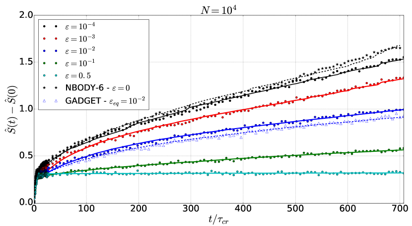
Regarding the discussion raised in §6.6 about the noisier appearance of the Fokker-Planck prediction for $N=10^{4}$ in comparison to larger $N$, it is interesting to see that for increasing $\varepsilon$ the prediction rapidly becomes smoother, even though the number of particles is fixed. This seems to indicate that the noise is not directly due to Poisson fluctuations of a small number of particles. Instead, since the introduction of a softening length suppresses encounters producing large scattering angles (even though not strictly close encounters, for which $b<b_{0}$, as shown above), the noise seems to be associated with the presence of a substantial number of such almost close encounters ($b\gtrsim b_{0}$, producing scattering angles $\lesssim 90^{\circ}$), what is expected for small $N$.

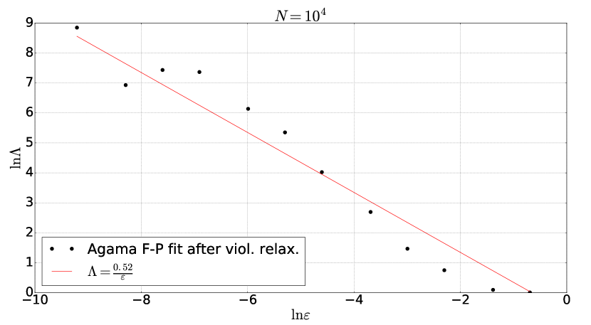
In Fig. 15 we show the Coulomb logarithm obtained fitting the Fokker-Planck equation to the entropy evolution for different $\varepsilon$ values (dots). The effect of suppression on 2-body relaxation for increasing softening length $\varepsilon$ can be parametrized in $\ln\Lambda$ substituting $b_{0}$ in Eq. (30) by an effective impact parameter ${b_{eff}=b_{min}+\varepsilon}$, where $b_{min}$ is expected to be of order of $b_{0}\approx R/N$, as suggested by Spinnato et al. (2003). The red curve shows the fit of $\ln\Lambda=\ln\left[b_{max}/(b_{min}+\varepsilon)\right]$, where $b_{max}$ and $b_{min}$ are free parameters, for which we get $b_{max}=0.52$ and $b_{min}\approx 0.0$. The value obtained for $b_{max}$ agrees with the assumption made in § 6.6, where we used $b_{max}=R_{hm}$. On the other hand, the value for $b_{min}$ is significantly smaller than expected, being compatible with zero. This seems to be associated to the fact that the first data point (smallest $\varepsilon$) is significantly higher than the expected trend of $\Lambda\approx const$ in this region.

Figure 15: Coulomb logarithm from the fit of orbit-averaged Fokker-Planck equation to the entropy evolution obtained with NBODY-2 for $N=10^{4}$ as a function of the softening length $\varepsilon$.

7 Conclusions

As discussed in §1, the validity of the Vlasov-Poisson equation implies the conservation of quantities defined by Eq. (7), for any functional $s[f]$ – see Tremaine et al. (1986). Conversely, non-conservation of any such quantity, like the Shannon entropy, implies non-validity of Vlasov-Poisson equation. In this paper, through the use of $N$-body simulations, we estimate the entropy at each time step, following its time evolution in order to test the validity of the Vlasov-Poisson equation for a collisionless self-gravitating system during violent relaxation.

Our results show a clear separation between the two relevant time scales: the dynamical time scale and the $2$-body relaxation time scale. During the early stages, in the dynamical time scale, the entropy has a significant increase accompanied by damping oscillations – see Fig. 2. This is the time scale in which the violent relaxation process is known to operate, the relaxation being associated to the typical particle interaction with the time-changing collective gravitational potential. This is the main result of this work, indicating that the Vlasov-Poisson equation does not seem to be valid during violent relaxation. This conclusion provides a natural solution to the so-called “fundamental paradox of stellar dynamics” (Ogorodnikov, 1965; Ossipkov, 2006). Several tests, changing the $N$-body simulation setups and estimators, as discussed in the preceding sections and commented below, lead to the same conclusion.

Instead of representing an exceptional situation, the entropy oscillations observed reinforce the reliability of our results, since they are typical of systems with considerable potential energy, as pointed out by Prigogine & Severne (1966); Jaynes (1971); Romero-Rochin & González-Tovar (1997). Moreover, Jaynes (1971) argues that the fact the “H” function is not monotonic can be associated to the non-validity of the hypothesis of molecular chaos, which is of fundamental importance in the derivation of the Vlasov-Poisson equation through the BBGKY hierarchy, a possibility also suggested by Beraldo e Silva et al. (2014).

Studying the impact of different initial conditions, the general conclusion is that entropy increase is higher for initial conditions farther from equilibrium. In particular, starting the simulation with the self-consistent Plummer model, which is a steady state, we see practically no entropy increase. This is in agreement with the general idea behind the statistical interpretation of the second law of Thermodynamics: that the systems evolve to the most probable state and that the entropy increase is due to the particular choice of a initial state which is very unlikely in comparison to the equilibrium state. The fact that we observe a negligible entropy increase in the case of initial Plummer model also weakens the possibility that the entropy increase observed in the other runs is being produced by some artificial, numerical relaxation.

Regarding the number of particles, we see in Fig. 4 that the early evolution of the entropy is qualitatively similar for $N=10^{4}$, $N=10^{5}$ and $N=10^{6}$. The more irregular appearance of the data points for $N=10^{4}$ can be attributed to shot noise due to the relatively small number of particles, while for $N=10^{5}$ and $N=10^{6}$ the curves are pretty smooth.

We note that oscillation amplitudes are larger for $N=10^{6}$ in comparison to $N=10^{5}$. This can be interpreted as follows: the $2$-body relaxation, although globally negligible for entropy increase already for $N=10^{5}$, can still act to destroy the coherent oscillatory pattern, smoothing out the curve, while for $N=10^{6}$ the $2$-body relaxation has even less effect, allowing the presence of coherent oscillations for a longer time period. This also reinforces the idea that convergence to significantly large $N$, i.e. to the collisionless regime, has been achieved for the time-scale of violent relaxation.

We also tested three different methods for estimating the distribution function: the Kernel method, Nearest Neighbor method and EnBiD (Sharma & Steinmetz, 2006). For $N=10^{5}$, Fig. 5 shows that Kernel and Nearest Neighbor have a general agreement with each other, but EnBiD shows some differences in respect to those methods, mainly a larger initial entropy production. Nevertheless, the general qualitative behaviour is similar for all these methods: a high entropy increase followed by damping oscillations in the dynamical time-scale. For $N=10^{6}$, Fig. 6 shows a much better agreement of all the methods, mainly between Kernel method and EnBiD with anisotropic kernel smoothing. This agreement suggests that the entropy evolution observed is not being produced by numerical artifacts but represents a good estimator for the true entropy evolution.

We also observe a good agreement for the entropy evolution obtained with the three different N-body simulation codes NBODY-6, NBODY-2 and GADGET-2 despite the fact the these codes involve different integration techniques. This reinforces the idea that the entropy evolution observed is not a numerical effect, but a real physical effect. Therefore, the results obtained from NBODY-2 with different values of the softening length $\varepsilon$ suggest that violent relaxation involves spatial scales around the mean neighboring particle distance, in agreement with the mathematical results summarized in Appendix A.

On the other hand, in the long-term, i.e. in the collisional relaxation time scale the entropy increases almost linearly. In order to verify if this entropy increase can be produced by $2$-body relaxation, we estimate the contribution of the orbit-averaged Fokker-Planck model to the entropy increase, Eqs. (18) and (27). Fig. 8 shows that this is the case indeed: if we restrict the fit to points after the early stages, say for $t/\tau_{cr}\gtrsim 26.5$, the Fokker-Planck model can reproduce quite accurately the almost linear entropy increase. However, not surprisingly, the orbit-averaged Fokker-Planck model cannot fit the early entropy evolution, during violent relaxation, where the potential is time-changing and the assumption $f=f(E)$ does not apply.

An interesting observation is that while the effectiveness of violent relaxation, i.e. the slope of $S(t)$, depends crucially on the initial conditions, the $2$-body relaxation seem to depend only on the number of particles $N$.

The variation of the softening length $\varepsilon$ in the long-term simulations generated with NBODY-2 also allowed us to study the characteristic scales for $2$-body relaxation. Our results seem to confirm that this relaxation process involve scales within the interval ${R/N\leq b\leq R}$.

In conclusion, our results show that during violent relaxation there is a significant entropy increase despite the prediction of the Vlasov-Poisson equation of entropy conservation. Under the assumption that the convergence for significantly large $N$ has been achieved (which seems to be the case), this early entropy increase cannot be attributed to any $2$-body relaxation process, and must be associated to a collective effect, which is the original idea behind violent relaxation.

These results indicate that the Vlasov-Poisson equation is not valid for collisionless self-gravitating systems during violent relaxation, resurrecting the arrow of time in the collapse of these systems.

Finally, the fact that the early regime with fast entropy changes extends up to $t\approx 25\tau_{cr}$, i.e. times substantially larger than $\tau_{cr}$ but still substantially smaller than $\tau_{col}$, can possibly support the collective relaxation time scale $\tau\propto N^{1/3}\tau_{cr}$ predicted by Gurzadian & Savvidy (1986). However, due to the reasonably weak $N$-dependence, a more rigorous test would require significantly larger numbers of particles.

8 Final remarks

The second law of Thermodynamics refers to the macroscopic evolution of any physical system, and does not depend on its on a description in terms of its microscopic constituents. Therefore, whenever a macroscopically irreversible evolution takes place, entropy is expected to increase. All results discussed in this work are in accordance with this idea.

On the other hand, when trying to explain the entropy evolution by means of a transport equation, it is important to keep in mind that even though the equation refers to the coordinates of one particle, it is not an equation of motion for some specific, randomly chosen, particle or fluid element. Instead, it statistically expresses the evolution of the system as a whole, referring to the coordinates of a statistical entity, the typical (or test) particle. As a result, it captures the influence of collective effects, which cannot be achieved using the equations of motion for a single particle. In this respect, any “transport equation” whose derivation is based only on mechanical considerations cannot describe the evolution of the system as a whole, but merely reassert the Hamiltonian evolution of each particle individually.

We should also mention that the right hand side of a transport equation is associated to any process relaxing the system, which only in the case of a molecular gas is necessarily realized by collisions, i.e. $2$-body interactions. This point is particularly important for a system with long-range interactions, which can relax even if it is collisionless. In fact, taking the presence of chaotic motions as a diagnostic of relaxation, it is interesting to remember that $N$-body self-gravitating systems can exhibit large (and increasing as $\ln N$) rates of growth of small perturbations, even for large $N$ – see Hemsendorf & Merritt (2002). In other words: these systems seem to be more chaotic for larger $N$, i.e. when they approach the collisionless regime – see also Kandrup & Sideris (2003).

The original statistical meaning of the distribution function seems to be frequently neglected, and in our opinion, the standard view of the necessity of a coarse-grain interpretation for the macroscopic evolution of the system serves to introduce this statistical meaning. This coarse-grain interpretation also seems to be reminiscent of discussions regarding the difference between Gibbs’s and Boltzmann’s definitions of entropy (Lebowitz, 1993a, b; Jaynes, 1965; Goldstein, 2001), which is in the heart of the opposition between the microscopic and macroscopic descriptions of the evolution of any system, not being restricted to the gravitational $N$-body problem. While Gibb’s entropy makes reference to the N-particle distribution function $f^{(N)}$, whose content is exclusively mechanical and is subject to Liouville’s equation $df^{(N)}/dt=0$, thus being conserved, Boltzmann’s entropy is defined in terms of the one-particle distribution function $f$, which has a statistical content and evolves in time. According to Jaynes (1965), “since the Gibbs H is dynamically constant, one has resorted to some kind of coarse-graining operation, resulting in a new quantity $\bar{H}$, which tends to decrease (…). Mathematically, the decrease in $\bar{H}$ is due only to the artificial coarse-graining operation and it cannot, therefore have any physical significance (…). The difference between H and $\bar{H}$ is characteristic, not of the macroscopic state, but of the particular way in which we choose to coarse-grain. Any really satisfactory demonstration of the second law must therefore be based on a different approach than coarse-graining”. As we can see, the standard coarse-grain interpretation is only necessary (though subject to criticism) when we adopt Gibbs’s entropy definition, i.e. in terms of $f^{(N)}$. However, if we adopt Boltzmann’s definition in terms of $f$, as done in this work, any possible coarse-grain interpretation is intrinsically there and any extra coarse graining is not necessary once we recognize the statistical content of the distribution function and abandon the assumption of validity of the Vlasov-Poisson equation during violent relaxation.

Appendix A Summary of mathematical results on the Vlasov-Poisson equation

For the Vlasov-Poisson initial value problem itself, there are various results (Pfaffelmoser, 1992; Schaeffer, 1991; Lions & Perthame, 1991; Horst, 1993) ensuring global existence and uniqueness of weak and strong solutions under fairly general conditions on the initial configuration. The first mathematically rigorous derivations of the Vlasov equation from a many-body problem can be found, e.g., in Neunzert & Wick (1974); Braun & Hepp (1977); Dobrushin (1979); Neunzert (1984). Rather than the Vlasov-Poisson equation, Neunzert & Wick (1974); Braun & Hepp (1977); Dobrushin (1979); Neunzert (1984); Spohn (2011) consider models with continuous and bounded forces. In particular, these forces are not diverging at small inter-particle distances $D$, in contrast to gravitational (Coulomb) forces. In the last few years progress has been made in treating mean field limits for forces which are singular at small distances up to but not including the Coulomb case. Hauray & Jabin (2015) discusses forces diverging as $\sim D^{-\alpha}$ with $\alpha<d-1$ in $d\geq 3$ dimensions. More precisely, in the case $1<\alpha<d-1$, a softening length of order $N^{-\frac{1}{2d}}$ is assumed in the derivation of the Vlasov equation from the $N$-body problem (Hauray & Jabin, 2015). If $\alpha<1$ no positive softening length is needed in the proof. Kiessling (2014) managed to prove a result including the Coulomb singularity under the assumption of an (uniform in $N$) a priori bound on the microscopic forces. However, whether it is satisfied for generic initial data or not, remains an open problem (Kiessling, 2014). Boers & Pickl (2016) improved the result of Hauray & Jabin (2015) in the sense that the softening length used is of order $N^{-\frac{1}{d}}$, but still $\alpha$ has to be strictly smaller than $d-1$ (and the Coulomb case is again not included). Recently, Lazarovici (2016); Lazarovici & Pickl (2017) extended the method of Boers & Pickl (2016) to include the Coulomb singularity, in 3 dimensions, aiming at a microscopic derivation of the Vlasov-Poisson dynamics. As in Hauray & Jabin (2015), a strictly positive softening length is needed, at fixed $N$. It can be chosen, as shown in Lazarovici & Pickl (2017), of order $N^{-\beta}$ with $\beta<\frac{1}{3}$.

These analyses suggest that inter-particle interactions taking place up to distances $d_{0}$ that are large compared to the mean neighboring particle distance $\bar{d}$, but small compared to the size of the whole system (i.e., scattering processes at impact parameters $b$ with $b\lesssim d_{0}$ and $\bar{d}\ll d_{0}\ll 1$), could prevent Vlasov-Poisson equation from being the effective macroscopic equation governing the evolution of collisionless self-gravitating systems. Note also that the long-range character of potentials is harmless in the mathematical derivation of Vlasov equations for $N$-body systems, as soon as their gradients (forces) are uniformly bounded at large distances. From this, we would not expect the emergence of the arrow of time in collisionless self-gravitating systems to be a consequence of scattering processes at large impact parameters.

Appendix B Some useful quantities and the Hénon units

The virial ratio is defined as

$$Q=-\frac{T}{W},$$ (B1)

where $T$ is total kinetic energy and $W$ is total potential energy. A convenient scale length is the virial radius $R_{vir}$ defined by

$$W=-\frac{GM^{2}}{2R_{vir}},$$ (B2)

where $G$ is the gravitational constant and $M$ is system’s total mass. The rms velocity is defined by

$$\langle v^{2}\rangle=\frac{2T}{M}=\frac{2(E-W)}{M},$$ (B3)

where $E$ is system’s total energy. The mean crossing time $\tau_{cr}$ is defined by

$$\tau_{cr}=\frac{2R_{vir}}{\sqrt{\langle v^{2}\rangle}}.$$ (B4)

The Hénon units (see Hénon, 1964), also called N-body units, are defined making $G=1$, $M=1$ and $E=-1/4$. Substituting in the above expressions, we obtain

$$R_{vir}=2(1-Q),$$ (B5)

$$\sqrt{\langle v^{2}\rangle}=\sqrt{\frac{Q}{2(1-Q)}}$$ (B6)

and thus

$$\tau_{cr}=4\sqrt{2}\sqrt{\frac{(1-Q)^{3}}{Q}}.$$ (B7)

In virial equilibrium, the total kinetic and potential energies respect

$$W=-2T,$$ (B8)

i.e. $Q=1/2$. Thus, in virial equilibrium, we have $R_{vir}=1$, $\langle v^{2}\rangle=1/2$ and finally $\tau_{cr}=2\sqrt{2}$.

Regarding the definition of the Plummer model, its density profile is given by

$$\rho(r)=\frac{3M}{4\pi a^{3}}\frac{1}{\left[1+\left(r/a\right)^{2}\right]^{5/2}},$$ (B9)

where $M$ is total mass and $a$ is a scale parameter. Thus, the radius containing half of the total mass is $R_{hm}\approx 1.3a$, and the total potential energy is $W=-3\pi GM^{2}/(32a)$. Substituting the $R_{vir}$ definition, Eq. (B2), we have $R_{vir}=16a/(3\pi)$. Thus, in the Plummer model $R_{hm}\approx 0.8R_{vir}$, and if the system is virialized, $R_{hm}\approx 0.8$ in Hénon units.

Regarding the impact parameter associated to a $90^{\circ}$ scattering angle,

$$b_{0}=\frac{G(m+m_{f})}{V^{2}},$$ (B10)

the relative velocity between the test and field particle is $\vec{V}=\vec{v}-\vec{v}_{f}$. Thus, $V^{2}=v^{2}+v_{f}^{2}-2\vec{v}\cdot\vec{v}_{f}$. Averaging over all particles of the system, we have $\langle V^{2}\rangle=\langle v^{2}\rangle+\langle v_{f}^{2}\rangle$. And if $m=m_{f}$, we have $\langle V^{2}\rangle=2\langle v^{2}\rangle$. Thus, for a virialized system composed of equal mass particles, we have

$$\Lambda=\frac{R_{hm}}{b_{0}}\approx 0.4N.$$ (B11)

References

- Aarseth (1999) Aarseth, S. 1999, in Bulletin of the American Astronomical Society, Vol. 31, AAS/Division of Dynamical Astronomy Meeting, 1226
- Aarseth (2001) Aarseth, S. J. 2001, New Astronomy, 6, 277
- Aarseth (2003) —. 2003, Gravitational N-Body Simulations, 430
- Aarseth et al. (1974) Aarseth, S. J., Henon, M., & Wielen, R. 1974, AAp, 37, 183
- Ahmad & Cohen (1973) Ahmad, A., & Cohen, L. 1973, JCP, 12, 389
- Ascasibar & Binney (2005) Ascasibar, Y., & Binney, J. 2005, MNRAS, 356, 872
- Balescu (1975) Balescu, R. 1975, Equilibrium and Non-Equilibrium Statistical Mechanics (John Wiley & Sons)
- Beirlant et al. (1997) Beirlant, J., Dudewicz, E. J., Györfi, L., & Van Der Meulen, E. C. 1997, International Journal of Mathematical and Statistical Sciences, 6, 17
- Beraldo e Silva et al. (2014) Beraldo e Silva, L., Lima, M., Sodré, L., & Perez, J. 2014, Phys. Rev. D, 90, 123004
- Bindoni & Secco (2008) Bindoni, D., & Secco, L. 2008, NAR, 52, 1
- Binney (1982) Binney, J. 1982, MNRAS, 201, 15
- Binney & Tremaine (2008) Binney, J., & Tremaine, S. 2008, Galactic Dynamics - Second Edition (Princeton University Press)
- Boers & Pickl (2016) Boers, N., & Pickl, P. 2016, JSP, 164, 1
- Braun & Hepp (1977) Braun, W., & Hepp, K. 1977, CMP, 56, 101
- Brush (1976) Brush, S. 1976, The kind of motion we call heat: a history of the kinetic theory of gases in the 19th century No. vol. 6,n.2 (North-Holland Pub. Co.)
- Chandrasekhar & von Neumann (1942) Chandrasekhar, S., & von Neumann, J. 1942, ApJ, 95, 489
- Chavanis (2013) Chavanis, P.-H. 2013, European Physical Journal Plus, 128, 126
- Colombi et al. (2015) Colombi, S., Sousbie, T., Peirani, S., Plum, G., & Suto, Y. 2015, MNRAS, 450, 3724
- Dobrushin (1979) Dobrushin, R. L. 1979, FAIA, 13, 115
- Efthymiopoulos et al. (2007) Efthymiopoulos, C., Voglis, N., & Kalapotharakos, C. 2007, in Lecture Notes in Physics, Vol. 729, Topics in Gravitational Dynamics, ed. D. Benest, C. Froeschle, & E. Lega (Springer Berlin Heidelberg), 297–389
- Ehrenfest & Ehrenfest (1959) Ehrenfest, P., & Ehrenfest, T. 1959, The conceptual foundations of the statistical approach in mechanics (Cornell University Press)
- Farouki & Salpeter (1982) Farouki, R. T., & Salpeter, E. E. 1982, ApJ, 253, 512
- Farouki & Salpeter (1994) —. 1994, ApJ, 427, 676
- Goldstein (2001) Goldstein, S. 2001, in Chance in Physics, Vol. 574, 39
- Gurzadian & Savvidy (1986) Gurzadian, V. G., & Savvidy, G. K. 1986, AAp, 160, 203
- Hahn & Angulo (2016) Hahn, O., & Angulo, R. E. 2016, MNRAS, 455, 1115
- Hall & Morton (1993) Hall, P., & Morton, S. C. 1993, AISM, 45, 69
- Hauray & Jabin (2015) Hauray, M., & Jabin, P.-E. 2015, Ann. Sci. de l’ENS, 48, 891
- Heggie & Hut (2003) Heggie, D., & Hut, P. 2003, The Gravitational Million-Body Problem: A Multidisciplinary Approach to Star Cluster Dynamics
- Hemsendorf & Merritt (2002) Hemsendorf, M., & Merritt, D. 2002, ApJ, 580, 606
- Hénon (1964) Hénon, M. 1964, Annales d’Astrophysique, 27, 83
- Hénon (1982) Hénon, M. 1982, AAP, 114, 211
- Hernquist & Barnes (1990) Hernquist, L., & Barnes, J. E. 1990, ApJ, 349, 562
- Horst (1993) Horst, E. 1993, MMAS, 16, 75
- Jaynes (1965) Jaynes, E. T. 1965, Am. J. Phys., 33, 391
- Jaynes (1971) —. 1971, PRA, 4, 747
- Joe (1989) Joe, H. 1989, AISM, 41, 683
- Kandrup (1980) Kandrup, H. E. 1980, Physics Reports, 63, 1
- Kandrup (1990) —. 1990, Physica A, 169, 73
- Kandrup (1998) Kandrup, H. E. 1998, Annals NY Academy of Sciences, 848, 28
- Kandrup et al. (1993) Kandrup, H. E., Mahon, M. E., & Smith, Jr., H. 1993, Astronomy and Astrophysics, 271, 440
- Kandrup & Sideris (2001) Kandrup, H. E., & Sideris, I. V. 2001, PRE, 64, 056209
- Kandrup & Sideris (2003) —. 2003, ApJ, 585, 244
- Kandrup et al. (2003) Kandrup, H. E., Vass, I. M., & Sideris, I. V. 2003, MNRAS, 341, 927
- Kiessling (2014) Kiessling, M. K.-H. 2014, JSP, 155, 1299
- King (1962) King, I. 1962, AJ, 67, 471
- Lazarovici (2016) Lazarovici, D. 2016, CMP, 347, 271
- Lazarovici & Pickl (2017) Lazarovici, D., & Pickl, P. 2017, Arch. Rat. Mech. Anal., doi:10.1007/s00205-017-1125-0
- Lebowitz (1993a) Lebowitz, J. L. 1993a, Physics Today, 46, 32
- Lebowitz (1993b) —. 1993b, Physica A, 194, 1
- Levin et al. (2014) Levin, Y., Pakter, R., Rizzato, F. B., Teles, T. N., & Benetti, F. P. C. 2014, Physics Reports, 535, 1
- Lifshitz & Pitaevskii (1980) Lifshitz, E. M., & Pitaevskii, L. P. 1980, Physical Kinetics (Butterworth–Heinemann)
- Lions & Perthame (1991) Lions, P. L., & Perthame, B. 1991, IM, 105, 415
- Lynden-Bell (1967) Lynden-Bell, D. 1967, MNRAS, 136, 101
- Maciejewski et al. (2009) Maciejewski, M., Colombi, S., Alard, C., Bouchet, F., & Pichon, C. 2009, MNRAS, 393, 703
- Madsen (1987) Madsen, J. 1987, ApJ, 316, 497
- Makino & Aarseth (1992) Makino, J., & Aarseth, S. J. 1992, PASJ, 44, 141
- Merritt (1999) Merritt, D. 1999, PASP, 111, 129
- Merritt (2005) —. 2005, Annals NY Acad. of Sciences, 1045, 3
- Merritt & Valluri (1996) Merritt, D., & Valluri, M. 1996, ApJ, 471, 82
- Monaghan & Lattanzio (1985) Monaghan, J. J., & Lattanzio, J. C. 1985, AAP, 149, 135
- Neunzert (1984) Neunzert, H. 1984, Lecture Notes in Mathematics, Berlin Springer Verlag, 1048, 60
- Neunzert & Wick (1974) Neunzert, H., & Wick, J. 1974, ZAMM, 54, 194
- Nitadori & Aarseth (2012) Nitadori, K., & Aarseth, S. J. 2012, MNRAS, 424, 545
- Ogorodnikov (1965) Ogorodnikov, K. F. 1965, Dynamics of stellar systems
- Ossipkov (2006) Ossipkov, L. P. 2006, AAT, 25, 123
- Padmanabhan (1990) Padmanabhan, T. 1990, Physics Reports, 188
- Pfaffelmoser (1992) Pfaffelmoser, K. 1992, JDE, 95, 281
- Prigogine & Severne (1966) Prigogine, I., & Severne, G. 1966, Physica, 32, 1376
- Romero-Rochin & González-Tovar (1997) Romero-Rochin, V., & González-Tovar, E. 1997, JSP, 89, 735
- Saslaw (1987) Saslaw, W. C. 1987, Gravitational Physics of Stellar and Galactic Systems
- Schaeffer (1991) Schaeffer, J. 1991, CPDE, 16, 1313
- Sellwood (2015) Sellwood, J. A. 2015, MNRAS, 453, 2919
- Sharma & Steinmetz (2006) Sharma, S., & Steinmetz, M. 2006, MNRAS, 373, 1293
- Shu (1978) Shu, F. H. 1978, ApJ, 225, 83
- Shu (1987) Shu, F. H. 1987, ApJ, 316, 502
- Silverman (1986) Silverman, B. W. 1986, Density estimation for statistics and data analysis
- Smith (1992) Smith, Jr., H. 1992, ApJ, 398, 519
- Spinnato et al. (2003) Spinnato, P. F., Fellhauer, M., & Portegies Zwart, S. F. 2003, MNRAS, 344, 22
- Spitzer (1987) Spitzer, L. 1987, Dynamical evolution of globular clusters
- Spohn (2011) Spohn, H. 2011, Large Scale Dynamics of Interacting Particles, Theoretical and Mathematical Physics (Springer Berlin Heidelberg)
- Springel (2005) Springel, V. 2005, MNRAS, 364, 1105
- Theis (1998) Theis, C. 1998, AA, 330, 1180
- Tremaine et al. (1986) Tremaine, S., Hénon, M., & Lynden-Bell, D. 1986, MNRAS, 219, 285
- Valluri & Merritt (1998) Valluri, M., & Merritt, D. 1998, ApJ, 506, 686
- Valluri & Merritt (2000) —. 2000, Advanced Series in Astrophysics and Cosmology, 10, 229
- Vasiliev (2015) Vasiliev, E. 2015, MNRAS, 446, 3150
- Vasiliev (2017 - submitted) —. 2017 - submitted
- Yoshikawa et al. (2013) Yoshikawa, K., Yoshida, N., & Umemura, M. 2013, APJ, 762, 116