On The Projection Operator to A Three-view Cardinality Constrained Set

Abstract

The cardinality constraint is an intrinsic way to restrict the solution structure in many domains, for example, sparse learning, feature selection, and compressed sensing. To solve a cardinality constrained problem, the key challenge is to solve the projection onto the cardinality constraint set, which is NP-hard in general when there exist multiple overlapped cardinality constraints. In this paper, we consider the scenario where the overlapped cardinality constraints satisfy a Three-view Cardinality Structure (TVCS), which reflects the natural restriction in many applications, such as identification of gene regulatory networks and task-worker assignment problem. We cast the projection into a linear programming, and show that for TVCS, the vertex solution of this linear programming is the solution for the original projection problem. We further prove that such solution can be found with the complexity proportional to the number of variables and constraints. We finally use synthetic experiments and two interesting applications in bioinformatics and crowdsourcing to validate the proposed TVCS model and method.

1 Introduction

The cardinality constraint is an intrinsic way to restrict the solution structure in many real problems, for example, sparse learning (Olshausen and Field, 1997), feature selection (Zhang, 2009), and compressed sensing (Candes et al., 2006). The generic cardinality constrained optimization can be expressed as

$$\min_{{\bf w}\in\mathbb{R}^{p}}\quad f({\bf w})$$ (1a)

subject to $$\|{\bf w}_{g}\|_{0}\leq{\bf s}^{g}\quad\forall g\in\mathcal{G}$$ (1b)

where ${\bf w}$ is the optimization variable, $g$ is an index subset of $[p]:=\{1,2,\cdots,p\}$, ${\bf w}_{g}$ is the sub-vector of ${\bf w}$ indexed by $g$. $\|{\bf w}_{g}\|_{0}$ denotes the cardinality of the sub-vector, i.e., the number of nonzeros in ${\bf w}_{g}$, $\mathcal{G}$ is the hyper set of all predefined groups, and ${\bf s}\in\mathbb{R}^{|\mathcal{G}|}$ is the upper bound vector - ${\bf s}^{g}\in\mathbb{R}$ refers to the upper bound of the sparsity over group $g$. Objective $f$ is the loss function which could be defined with different form according to the specific application. The problem (1) refers to a nonconvex optimization (NP-hard) due to the cardinality constraint. Some efficient iterative methods such as IHT (Yuan et al., 2014), CoSaMP (Needell and Tropp, 2009), GradMP (Nguyen et al., 2012), and their variants can guarantee to solve the original problem under some mild conditions. A key component in all of these methods is the projection operator

$$\text{P}_{\Omega(\mathcal{G},{\bf s})}({\bf v}):=\operatorname*{arg\,min}_{{\bf w}\in\Omega(\mathcal{G},{\bf s})}\quad \|{\bf w}-{\bf v}\|^{2}$$ (2)

where $\Omega(\mathcal{G},{\bf s})$ denotes the feasible set to the constraint (1b). While in some special case, for example, $\mathcal{G}=\{[p]\}$, the projection is trivial, it is quite challenging, especially when $\mathcal{G}$ includes multiple overlapped index sets (even NP-hard in some cases).

In this paper, we consider the scenario where the overlapped cardinality constraints (1b) satisfy a Three-view Cardinality Structure (TVCS):

Definition 1.

(Three-view Cardinality Structure (TVCS)) For $\Omega(\mathcal{G},{\bf s})$, the hyper set $\mathcal{G}$ consisting of subsets of $[p]$ admits the TVCS structure if the following conditions are satisfied:

• There exists a partition $\mathcal{G}_{0}$, $\mathcal{G}_{1}$ and $\mathcal{G}_{2}$ such that $\mathcal{G}=\mathcal{G}_{0}\cup\mathcal{G}_{1}\cup\mathcal{G}_{2}$;

• $\mathcal{G}_{0}=\{[p]\}$;

• All element sets in $\mathcal{G}_{1}$ have no overlap;

• All element sets in $\mathcal{G}_{2}$ have no overlap.

This definition basically requires that $\mathcal{G}$ can be partitioned into three hyper sets $\mathcal{G}_{0}$, $\mathcal{G}_{1}$, and $\mathcal{G}_{2}$, and overlaps can only happen between element sets in different hyper sets. $\mathcal{G}_{0}$ is usually used to restrict the overall sparsity. Figure 1 provides two examples of $\mathcal{G}$ for TVCS.

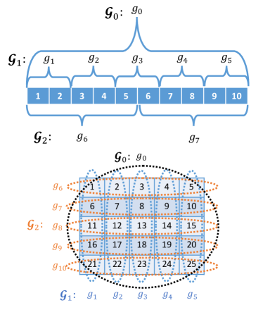
Figure 1: Two examples of groups for TVCS model. The first model has $p=10$, $\mathcal{G}_{0}=\{g_{0}\},\mathcal{G}_{1}=\{g_{1},g_{2},g_{3},g_{4},g_{5}\},\mathcal{G}_{2}=\{g_{6},g_{7}\}$. The second model organizes elements as matrix ($p=25$). Each row and column is a group, and $\mathcal{G}_{0}=\{g_{0}\},\mathcal{G}_{1}=\{g_{1},g_{2},g_{3},g_{4},g_{5}\},\mathcal{G}_{2}=\{g_{6},g_{7},g_{8},g_{9},g_{10}\}$.

The TVCS model is motivated from some important applications, for example, in recommendation, task-worker assignment, and bioinformatics.

• Online recommendation. Suppose we want to recommend a certain number of books (among $p$ books) to a customer - corresponding to the $\mathcal{G}_{0}$ based sparsity constraint. Among the selected books, we want to maintain some diversities - the recommended books by the same author should not exceed a certain number ($\mathcal{G}_{1}$ based sparsity constraint) and about the same topic should not exceed a certain number either ($\mathcal{G}_{2}$ based sparsity constraint). One can refer to the top graph in Figure 1: $\mathcal{G}_{1}$ is grouped by authors and $\mathcal{G}_{2}$ is grouped by topics.

• Task-worker assignment. Suppose we have a bunch of tasks and workers, and we want to assign the tasks to workers. For example, in crowdsourcing, we usually assign several different workers to each task since we want to use the answers from multiple workers to improve the accuracy. On the other hand, each worker is usually assigned to multiple tasks so there is a “many to many” relationship in this assignment. The goal is to pursue the optimal assignment under a certain criteria in crowdsourcing, while satisfying some restrictions. For example, the total assignments should be bounded by the total budget (corresponding to $\mathcal{G}_{0}$), the total cost of assignments to a single worker cannot exceed a certain threshold (corresponding to $\mathcal{G}_{1}$), and the total cost of assignments on a single task cannot exceed a certain threshold (corresponding to $\mathcal{G}_{2}$). Let $X$ be the assignment matrix, and its rows are indexed by workers and the columns are indexed by tasks. These constraints can be illustrated by the bottom graph in Figure 1.

• Identification of gene regulatory networks. The essential goal of identifying gene regulatory network is to identify a weighted directed graph, which can be represented by a square matrix $W$ with $p=N\times N$ elements in total where $N$ is the number of vertices. A sparse network constraint is to restrict the in-degree and out-degree for each vertex, which corresponds to the sparsity in each row and column of $W$.

To solve the TVCS constrained projection (2), we show an interesting connection between the projection and a linear programming (LP) that the vertex solution to this linear programming is an integer solution which solves the original problem.

To find an integer solution to such LP efficiently, we formulate it into a feasibility problem, and further an equivalent quadratic convex optimization. By using the rounding technique, we can avoid solving the exact solution of this LP problem. We propose an iterative algorithm to solve it and each iteration can be completed in linear time. We also show that the iterate linearly converges to the optimal point. Finally, the proposed TVCS model is validated by the synthetic experiment and two important and novel applications in identification of gene regulatory networks and task assignment problem of crowdsourcing.

2 Related Works

Recent years have witnessed many research works in the field of structured sparsity and group-based sparsity. Yuan and Lin (2006) introduced the group LASSO, which pursues group-wise sparsity that restricts the number of groups for the selected variables. Jenatton et al. (2011) construct a hierarchical structure over the variables and use group LASSO with overlapped groups to solve it. Exclusive LASSO (Zhou et al., 2010; Kong et al., 2014) was proposed for the exclusive group sparsity which can be treated as relaxing our cardinality constraints to convex regularizations. In (Kong et al., 2014), the authors discussed the overlapping situation and tried to solve the problem using convex relaxation, which is different from our approach. Besides the aforementioned works, some proposed more general models to cover various sparsity structures. Bach et al. (2012) extended the usage of $L_{1}$-norm relaxation to several different categories of structures. And recently, another generalization work (El Halabi and Cevher, 2015) proposed convex envelopes for various sparsity structures. They built the framework by defining a totally unimodular penalty, and showed how to formulate different sparsity structures using the penalty. The work above concentrated on using convex relaxation to control the sparsity.

Besides using convex relaxation, there are also some works focusing on projection-based methods. When the exact projection operator was provided, Baraniuk et al. (2010) extended the traditional IHT and CoSaMP methods to general sparsity structures. In this work, the authors also introduced the projection operator for block sparsity and tree sparsity. Cevher et al. (2009) investigated cluster sparsity and they applied dynamic programming to solve the projection operator for their sparsity model. Hegde et al. (2009) introduced a “spike trains” signal model, which is also related to exclusive group sparsity. Its groups always have consecutive coordinates, and each group cannot contain more than one nonzero element. To solve the projection problem of their model, they showed the basic feasible solutions of the relaxed linear programming (LP) are always integer points. In our work, we also use LP to solve the projection problem. But our model defines the group structure differently and aims at different applications.

In addition, there are some works for the cases without an efficient exact projection operator (Hegde et al., 2015a, b; Nguyen et al., 2014). This is meaningful since the projection operator for complex structured sparsity often involves solving complicated combinatorial optimization problems. Hegde et al. (2015a) discussed how to guarantee convergence if using approximate projection in IHT and CoSaMP for compressive sensing. They proved that the convergence needs a “head approximation” to project the update (gradient) before applying it. Hegde et al. (2015b) proposed a general framework to formulate a series of models as a weighted graph, and designed an efficient approximate projection operator for the models. Nguyen et al. (2014) applied the approximate projection-based IHT and CoSaMP to general convex functions and stochastic gradients.

3 Preliminary: GradMP and IHT Frameworks

This section briefly reviews two commonly used algorithm frameworks to solve the cardinality constrained optimization (1): iterative hard thresholding (IHT) (Yuan et al., 2014; Nguyen et al., 2014) and gradient matching pursuit (GradMP) (Nguyen et al., 2012, 2014) (the general version of CoSaMP (Needell and Tropp, 2009)) for solving cardinality constrained problem. Other methods like hard thresholding pursuit (HTP) also follows similar steps and has been shown to be effective both empirically and theoretically (Yuan et al., 2016). The procedures of IHT and GradMP for our model are shown in Algorithms 1 and 2, where $\text{supp}(\cdot)$ is the support set of the argument vector.

Therefore, one can see that the efficiency of both algorithms relies on the computation of the gradient and the projection. To avoid the expensive computation of the gradient, GradMP and IHT can be extended to the stochastic versions (Nguyen et al., 2014) by assigning ${\bf g}$ the stochastic gradient at the gradient computation step.

Both Algorithms 1 and  2 (and their stochastic variants) guarantee some nice properties: the iterate converges to a small ball surrounding the true solution at a linear rate under certain RIP-type conditions (Nguyen et al., 2014) and the radius of such ball converges to zero when the number of samples goes to infinity.

Input: Sparsity parameter ${\bf s}$.

Result: Problem solution ${\bf w}^{t}$.

Initialize ${\bf w}^{0},t=0$;

while stop criterion is not met do

       ${\bf g}={\nabla}f({\bf w}^{t})$ ;

        // Gradient computation

       ${\bf z}^{t}={\bf w}^{t}-\gamma{\bf g}$ ;

        // Gradient descent

       ${\bf w}^{t+1}=\text{P}_{\Omega(\mathcal{G},{\bf s})}({\bf z}^{t})$ ;

        // Projection

       $t=t+1$;

      

end while

Algorithm 1 Iterative Hard Thresholding.

Input: Sparsity parameter ${\bf s}$.

Result: Problem solution ${\bf w}^{t}$.

Initialize ${\bf w}^{0},t=0$;

while stop criterion is not met do

       ${\bf g}=\nabla f({\bf w}^{t})$;

        // Gradient computation

       $\Gamma=\text{supp}(\text{P}_{\Omega(\mathcal{G},2{\bf s})}({\bf g}))$;

       $\hat{\Gamma}=\Gamma\cup\text{supp}({\bf w}^{t})$ ;

        // Subspace selection

       ${\bf z}^{t}=\operatorname*{arg\,min}_{\text{supp}({\bf z})=\hat{\Gamma}}f({\bf z})$ ;

        // Subspace optimization

       ${\bf w}^{t+1}=\text{P}_{\Omega(\mathcal{G},{\bf s})}({\bf z}^{t})$ ;

        // Projection

       $t=t+1$;

      

end while

Algorithm 2 Gradient Matching Pursuit.

A common component in Algorithms 1 and 2 is the projection operator. If all the groups except $[p]$ in $\mathcal{G}$ do not overlap each other, the projection problem can be easily solved by sequential projections (Yang et al., 2016). But for those cases involving overlapped groups, it is generally challenging to solve them efficiently.

4 Projection Operator

This section introduces how to solve the essential projection step. Note that the projection onto a nonconvex set is NP-hard in general. By utilizing the special structure of TVCS, we show that the projection can be solved efficiently. Due to the page limitation, all proofs are provided in the supplementary material.

4.1 LP Relaxation

Firstly, we can cast the projection problem (2) to an equivalent integer linear programming problem (ILP) according to Lemma 1.

Lemma 1.

The projection problem (2) is equivalent to the following integer linear programming problem (ILP):

$$\max_{\bf x}\quad \langle{\bf v}^{2},{\bf x}\rangle$$ (3)

subject to $$A{\bf x}\leq{\bf s}$$

$${{\bf x}\in\{0,1\}^{p}}$$

where ${\bf v}^{2}$ is applying element-wise square operation on vector ${\bf v}$. $A$ is a $|\mathcal{G}|\times p$ matrix which is defined as:

$$A=\begin{bmatrix}{\bf{1}}^{\top}\\ C\end{bmatrix}$$ (4)

where $C\in\{0,1\}^{|\mathcal{G}_{1}\cup\mathcal{G}_{2}|\times p}$, whose rows represent the indicator vector of each group $g\in\mathcal{G}_{1}$ and $\mathcal{G}_{2}$.

Each row in $A$ corresponds to one group $g$ from $\mathcal{G}$. For example, $C_{ij}=1$ if the $j$-th coordinate is in the $i$-th group, otherwise $C_{ij}=0$. The first row ${\bf{1}}^{\top}$ corresponds to the overall sparsity i.e. $\mathcal{G}_{0}$.

It is NP-hard to solve an ILP in general. One common way to handle such ILP is making a linear programming (LP) relaxation. In our case, we can use a box constraint ${\bf x}\in[0,1]^{p}$ to replace the integer constraint ${\bf x}\in\{0,1\}^{p}$:

$$\max_{\bf x}\quad \langle{\bf v}^{2},{\bf x}\rangle$$ (5)

subject to $$A{\bf x}\leq{\bf s}$$

$${{\bf x}\in[0,1]^{p}}$$

However, there is no guarantee that a general ILP can be solved via its LP relaxation, because the solution of the relaxed LP is not always integer. Although one can make a rounding to the LP solution and acquire a integer solution, such solution is not guaranteed to be optimal (or even feasible) to the original ILP.

Fortunately, due to the special structure of our TVCS model, we find that its relaxed LP has some nice properties which make it possible to get the optimal solution of the ILP efficiently. The following theorem reveals the relationship between the ILP problem and the relaxed LP problem.

Theorem 2.

Given $\mathcal{G}$ satisfying $TVCS$, all the vertices of the feasible set to (5) are integer points. Furthermore, there is an optimal solution on the vertex that solves the ILP (3).

This theorem suggests that finding a vertex solution of the relaxed LP can solve the original projection problem onto a TVCS $\mathcal{G}$. The proof basically shows that matrix $A$ (for TVCS) is a totally unimodular matrix (Papadimitriou and Steiglitz, 1982). We provide the detailed proof in the supplementary material.

4.2 Linearly Convergent Algorithm for Projection Operator onto TVCS

To find a solution on the vertex, one can use the Simplex method. Although Simplex method guarantees to find an optimal solution on the vertex and could be very efficient in practice, it does not have a deterministic complexity bound. In the IHT and GradMP algorithms, projection operator is only a sub-procedure in one iteration. Hence, we are usually supposed to solve lots of instances of problem (3). Simplex might be efficient practically, but its worst case may lead to exponential time complexity (Papadimitriou and Steiglitz, 1982). In this section, the integer solution to the linear programming can be found within the complexity proportional to the number of variables and constraints.

Equivalent Feasibility Problem Formulation.

The dual of LP problem (5) can be written as:

$$\min_{\bf y}\quad \langle[{\bf s}^{\top}\ {\bf{1}}^{\top}]^{\top},{\bf y}\rangle$$ (6)

subject to $$\begin{bmatrix}A^{\top}\ I\end{bmatrix}{\bf y}\geq{\bf v}^{2},{\bf y}\geq{\bf{0}}$$

Since the duality gap of LP is zero, combining the primal LP (5) and dual LP (6), we can formulate an equivalent problem, i.e. the feasibility problem over the following constraints:

find $${\bf x},{\bf y}$$

subject to $$\langle[{\bf s}^{\top}\ {\bf{1}}^{\top}]^{\top},{\bf y}\rangle=\langle{\bf v}^{2},{\bf x}\rangle$$

$$\begin{bmatrix}A^{\top}\ I\end{bmatrix}{\bf y}\geq{\bf v}^{2}$$

$$\begin{bmatrix}A\\ I\end{bmatrix}{\bf x}\leq\begin{bmatrix}{\bf s}\\ {\bf{1}}\end{bmatrix}$$

$${\bf y}\geq{\bf{0}},{\bf x}\geq{\bf{0}}$$

Iterative Algorithm.

The feasibility problem with linear constraints above is equivalent to the following optimization problem:

$$\min_{{\bf x},{\bf y}}\quad {1\over 2}(\langle[{\bf s}^{\top}\ {\bf{1}}^{\top}]^{\top},{\bf y}\rangle-\langle{\bf v}^{2},{\bf x}\rangle)^{2}$$

$$+{1\over 2}\|[{\bf v}^{2}-[A^{\top}\ I]{\bf y}]_{+}\|^{2}+{1\over 2}\|[A{\bf x}-{\bf s}]_{+}\|^{2}$$ (7)

subject to $${\bf{0}}\leq{\bf x}\leq{\bf{1}},{\bf y}\geq 0$$

where $[{\bf z}]_{+}$ is the element-wise hinge operator, i.e. it transforms each element ${\bf z}_{i}$ to $\max({\bf z}_{i},0)$.

This is a convex optimization problem with a quadratic objective and box constraints. We adopt the projected gradient descent to solve this problem, and show it converges linearly.

Theorem 3.

For the optimization problem with the form

$$\min_{\bf z}\quad f({\bf z}):=\|[A{\bf z}-a]_{+}\|^{2}+\|B{\bf z}-b\|^{2}$$

subject to $${\bf z}\in\Omega$$

where $\Omega=\{{\bf z}\mid C{\bf z}\leq c\}$, the projected gradient descent algorithm ${\bf z}^{t+1}\leftarrow P_{\Omega}({\bf z}^{t}-\gamma\nabla f({\bf z}^{t}))$ has a linear convergence rate with some $\alpha<1$ (depending on $A$ and $B$):

$$\|{\bf z}^{t+1}-P_{{\bf z}^{*}}({\bf z}^{t+1})\|\leq\alpha\|{\bf z}^{t}-P_{{\bf z}^{*}}({\bf z}^{t})\|,$$

where $P_{{\bf z}^{*}}(\cdot)$ is the projection onto the optimal solution set.

Notice that the objective function $f$ in Theorem 3 is not necessarily strongly convex, which means the well recognized linear convergence conclusion from the strong convexity is not applicable here.

Theorem 3 mainly applies Hoffman’s Theorem (Hoffman, 2003) to show that $f$ is an optimal strongly convex function (Liu and Wright, 2015). This leads to a linear convergence rate.

The convergence rate $\alpha=\nicefrac{{1}}{{(1+{\lambda\over L})}}$, where $\lambda$ is the Hoffman constant (Hoffman, 2003) that depends on $A,B$ and is always positive. $L$ is the Lipschitz continuous gradient constant. More details are included in the supplementary materials.

To show the complexity of this algorithm, we firstly count how many iterations we need. Since we know that we can just make a rounding to the result ${\bf x}^{t}$ when we attain $\|{\bf x}^{t}-\tilde{{\bf x}}^{*}\|_{\infty}<0.5$. Let ${\bf z}:=[{\bf x}^{\top}\ {\bf y}^{\top}]^{\top}$ represent all the variables in (7). Because $\|{\bf z}^{t}-{{\bf z}}^{*}\|\geq\|{\bf z}^{t}-{{\bf z}}^{*}\|_{\infty}\geq\|{\bf x}^{t}-{{\bf x}}^{*}\|_{\infty}$, we can do the rounding safely when $\|{\bf z}^{t}-{{\bf z}}^{*}\|<0.5$, where ${{\bf z}}^{*},{{\bf x}}^{*}$ are the optimal points of this problem. According to Theorem 3, we have the linear convergence rate $\alpha<1$, so the number of iterations we need is

$$t>\log_{\alpha}{1\over 2\|{\bf z}^{0}-{{\bf z}}^{*}\|}$$

Therefore, we claim that we can obtain the solution ${{\bf x}}^{*}$ by rounding after $\log_{\alpha}{1\over 2\|{\bf z}^{0}-{{\bf z}}^{*}\|}$ iterations.

Secondly, we show that the computation complexity in each iteration is linear with dimensionality $p$ and the amount of groups $|\mathcal{G}|$. Since each column of $A$ contains at most 3 nonzero elements, the complexity of the matrix multiplications in computing the gradient of (7) is $O(p+|\mathcal{G}|)$. Together with other computation, the complexity for each iteration is $O(p+|\mathcal{G}|)$.

5 Empirical Study

This section will validate the proposed method on both synthetic data and two practical applications: crowdsourcing and identification of gene regulatory networks.

5.1 Linear Regression and Classification on Synthetic Data

In this section, we validate the proposed method with linear regression objective and squared hinge objective (classification) on synthetic data. Let ${\bf w}\in\mathbb{R}^{\sqrt{p}\times\sqrt{p}}$ be a matrix, $\mathcal{G}_{1}$ and $\mathcal{G}_{2}$ are defined as groups with all rows and all columns respectively. The linear regression loss is defined as $\sum_{i=1}^{n}(\langle X_{i},{\bf w}\rangle-y_{i})^{2}$ and the squared hinge loss is defined as $\sum_{i=1}^{n}\max(0,1-y_{i}\langle X_{i},{\bf w}\rangle)^{2}$, where $n$ is the total number of training samples. $X_{i}$ and $y_{i}$ are the features and label of the $i$-th sample respectively.

In the linear regression experiment, the true model $\bar{{\bf w}}\in\mathbb{R}^{\sqrt{p}\times\sqrt{p}}$ is generated from the following procedure: generate a random vector and apply the projection operator to get a support set which satisfy our sparsity constraints; the elements of positions in support set are drawn from standard normal distribution. $p$ is fixed as $400$ and $n$ is gradually increased. The group sparsity upper bounds ${\bf s}^{g}$ for $g\in\mathcal{G}_{1}$ and $g\in\mathcal{G}_{2}$ are uniformly generated from the integers in the range$[1,\sqrt{p}]$. The overall sparsity upper bound is set by $0.8\times\min(\sum_{g\in\mathcal{G}_{1}}{\bf s}^{g},\sum_{g\in\mathcal{G}_{2}}{\bf s}^{g})$. Each $X_{i}$’s is an $\sqrt{p}\times\sqrt{p}$ i.i.d. Gaussian random matrix. $y_{i}$ is generated from $y_{i}=\langle X_{i},\bar{{\bf w}}\rangle+e_{i}$, where $e_{i}$ is the i.i.d. Gaussian random noise drawn from $\mathcal{N}(0,0.01^{2})$. We compare the proposed methods to bilevel exclusive sparsity with non-overlapped groups (row-wise or column-wise) (Yang et al., 2016), overall sparsity (Needell and Tropp, 2009), and exclusive LASSO (Kong et al., 2014). For fairness we project the final result of all the compared methods to satisfy all constraints. All the experiments are repeated 30 times and we use the averaged result. We use selection recall and successful recovery rate to evaluate the performance. Selection recall is defined as $\nicefrac{{|\text{supp}({\bf w}^{*})\cap\text{supp}(\bar{{\bf w}})|}}{{\|\bar{{\bf w}}\|_{0}}}$, where ${\bf w}^{*}$ is the optimization result. Successful recovery rate is the ratio of the successful feature selection i.e. $\text{supp}({\bf w}^{*})=\text{supp}(\bar{{\bf w}})$ to the total number of repeated experiments. In Figure 2 we can observe that our model with all sparsity constraints always have the best performance. While the performance of exclusive LASSO and our method is comparable when the number of samples are very limited, our method outperforms exclusive LASSO when the number of samples increases.

For classification experiments, we use the same settings of sparsity with linear regression. Here we set $p=400$, and change $n$ from $200$ to $800$. The true model $\bar{{\bf w}}$ and feature matrices are generated by the same way as the linear regression experiment. The class label $y_{i}\in\{-1,1\}$ is got by $y_{i}=\text{sign}\langle X_{i},\bar{{\bf w}}\rangle$. Besides the selection recall, we also compare the classification error. In Figure 3, we can see that the superiority of our method is even more significant in the classification experiment. Although the overall sparsity has the lowest selection recall, it still has a similar classification error with the methods that consider row or column groups.

(a) Selection recall.

(b) Successful recovery rate.

Figure 2: Selection recall and successful recovery rate for least square loss.

(a) Selection recall.

(b) Classification error.

Figure 3: Selection recall and classification error for squared hinge loss.

5.2 Application in Crowdsourcing

This section applies the proposed method to the worker-task assignment problem in crowdsourcing. Take the image labeling task as an example. Given $n$ workers and $m$ images, each image can be assigned to multiple workers and each worker can label multiple images. The predicted label for each image is decided by all the labels provided by the assigned workers and the quality of each worker on the image. The goal is to maximize the expected prediction accuracy based on the assignment. Let $X\in\{0,1\}^{n\times m}$ be the assignment matrix, i.e. $X_{ij}=1$ if assign the $i$-th worker to $j$-th task, otherwise $X_{ij}=0$. $Q\in[0,1]^{n\times m}$ is the corresponding quality matrix, which is usually estimated from the golden standard test (Ho et al., 2013). The whole formulation is defined to maximize the average of the expected prediction accuracy over $m$ tasks over a TVCS constraint:

$$\max_{X}\quad {1\over m}\sum_{j=1}^{m}\mathcal{E}_{\text{acc}}(Q_{\cdot,j},X_{\cdot,j})$$ (8)

subject to $$\sum_{i=1}^{n}X_{ij}\leq{\bf s}^{\text{worker}},\forall j;$$

$$\sum_{j=1}^{m}X_{ij}\leq{\bf s}^{\text{task}},\forall i;$$

$$\sum_{i,j}X_{ij}\leq{\bf s}^{\text{total}};\ X\in\{0,1\}^{n\times m}$$

where $\mathcal{E}_{\text{acc}}(\cdot,\cdot)$ is the expected prediction accuracy, ${\bf s}^{\text{worker}}$ is the “worker sparsity”, i.e. the largest number of assigned workers for each task, and ${\bf s}^{\text{task}}$ is the “task sparsity”, i.e. each worker can be assigned with at most ${\bf s}^{\text{task}}$ tasks, and ${\bf s}^{\text{total}}$ is the total sparsity to control the budget, i.e., the maximal number of assignment. In image labeling task, we assume that each image can only have two possible classes and the percentage of images in each class is one half. We use the Bayesian rule to infer the predicted labels given the workers’ answer. Here we consider the binary classification task. Let ${\bf y}_{j}\in\{1,0\}$ be the true label of the $j$-th task and $\hat{{\bf y}}_{j}$ be the prediction given labels by selected workers, i.e.,

$$\hat{{\bf y}}_{j}=\begin{cases}0,&\text{ if }\mathbb{P}({\bf y}_{j}=1|\hat{Y}_{\Omega_{j},j})<\mathbb{P}({\bf y}_{j}=0|\hat{Y}_{\Omega_{j},j});\\ 1,&\text{ otherwise }\end{cases}$$

where $\hat{Y}_{ij}$ is the $i$-th worker’s predication on $j$-th task. Set $\Omega_{j}$ contains the indices of the selected workers for $j$-th task, i.e. $X_{ij}=1,\forall i\in\Omega_{j}$, and $X_{i^{\prime}j}=0,\forall i^{\prime}\notin\Omega_{j}$

Then $\mathcal{E}_{\text{acc}}(Q_{\cdot,j},X_{\cdot,j})$ can be defined in the following:

$$\mathcal{E}_{\text{acc}}(Q_{\cdot,j},X_{\cdot,j})=\mathbb{P}(\hat{{\bf y}}_{j}=1,{\bf y}_{j}=1)+\mathbb{P}(\hat{{\bf y}}_{j}=0,{\bf y}_{j}=0)$$

By this way, the expected accuracy will not be continuous, so we use smooth function to approximate the expected accuracy and adopt the stochastic gradient with the proposed projection operator to optimize it. Due to the space limitation, the detailed derivation of the objective formulation can be found in the supplemental material.

We conduct experiment for crowdsourcing task assignment on synthetic data. Specifically, we generate the quality matrix $Q$ from uniformly random distribution with interval $[0.5,0.9]$. The prior probability $\mathbb{P}({\bf y}_{j}=1)$ and $\mathbb{P}({\bf y}_{j}=0)$ are set as $0.5$ for all the tasks.

To avoid evaluating the expectation term, we apply the stochastic iterative hard thresholding framework (Nguyen et al., 2014). Each iteration we get $\hat{Y}|{\bf y}_{j}=1$ and $\hat{Y}|{\bf y}_{j}=0$ by sampling based on $Q$ i.e. $\mathbb{P}(\hat{Y}_{ij}=1|{\bf y}_{j}=1)=Q_{ij}$, $\mathbb{P}(\hat{Y}_{ij}=0|{\bf y}_{j}=0)=Q_{ij}$. Then we can get a stochastic gradient based on the sampled $\hat{Y}$.

(a) $n=100$, $m=1,000$.

(b) $n=200$, $m=10,000$.

Figure 4: Expected accuracy of crowdsourced classification.

Besides the proposed formulation (8), we evaluate the random assignment algorithm and the Q-based linear programming (Ho et al., 2013). The random assignment algorithm widely used in practice is the most straightforward approach: given the total assignment budget ${\bf s}^{\text{total}}$ and the restrictions (${\bf s}^{\text{worker}}$ and ${\bf s}^{\text{task}}$) for workers and tasks, randomly assign tasks to the workers. The Q-based linear programming uses the linear combination of $Q_{ij}$ over $i$ to evaluate the overall accuracy on task $j$ for simpler formulation. In addition, it does not consider the restriction on tasks, thus it may assign lots of workers to a difficult task. To make a fair comparison, the task restriction is added into this method. To get the assignment result which satisfies the task and worker restriction, we use our projection operator in the other methods too.

We evaluate the experiments on different value of ${\bf s}^{\text{task}},{\bf s}^{\text{worker}}$ by setting them as different ratios of the total number of tasks and workers. The overall sparsity is set by the same way as in Section 5.1. To measure the performance, we compare the sampled expected accuracy. The samples (i.e., $\hat{Y}$) are independent to the samples used in training. Figure 4 shows the comparison of the expected accuracy of the three approaches. We can observe that the accuracy increases with larger ratio (i.e. more assignments). The random assignment strategy needs more assignments to get the same accuracy compared with the other two methods.

5.3 Application in Identification of Gene Regulatory Networks

In this section, we apply the projection operator to the identification of gene regulatory networks (GRN).

Background.

Gene regulatory network represents the relations between different genes, which plays important roles in biological processes and activities by controlling the expression level of RNAs. There is a well-known biological competition named DREAM challenge about identifying GRN. Based on the time series gene expression data which are RNAs’ level along time sequence, contestants are required to recover the whole gene network of given size. One popular way to infer GRN is to utilize the sparse property of GRN: e.g., one gene in the network is only related to a small number of genes and we already know that there exists no relationship between some genes. Therefore, the amount of edges connecting to one vertex is far less than the dimension of the graph. It is a practical case of row-wise and column-wise sparsity for matrix. We could apply the projection operator to constrain the number of edges related to each vertex to identify the whole network. Recently, the dynamic Bayesian network (DBN) (Zou and Conzen, 2005) is supposed to be an effective model to recover GRNs. The RNAs’ level of all genes in GRN at time $t$ is stored in gene expression vector $\textbf{x}_{t}\in\mathbb{R}^{N}$, where each entry corresponds to one gene respectively and $N$ is the number of genes in GRN. Hence, We define the total amount of time points in the experiment as $T$. Gene activity model is usually assumed to be

$${\bf x}_{t+1}=P{\bf x}_{t}+{\bf e}_{t},\quad t=1\ldots T-1,$$

where $P\in\mathbb{R}^{N\times N}$ is the covariance matrix of GRN and ${\bf e}_{t}\in\mathbb{R}^{N}$ is Gaussian white noise. Then the difference of RNA levels between time points $t+1$ and $t$, i.e. ${\bf y}_{t+1,t}\in\mathbb{R}^{N}$ is defined as follows:

$${\bf y}_{t+1,t}:={\bf x}_{t+1}-{\bf x}_{t}=\bar{{W}}{\bf x}_{t}+{\bf e}_{t},\quad t=1\ldots T-1,$$

where $\bar{{W}}=P-I$ is the true sparse $N$-by-$N$ matrix. Therefore, the GRN is only considered between different genes and we eliminate edges whose start and end vertex are the same. We define that $Y:=[{\bf y}_{2,1},\ldots,{\bf y}_{T,T-1}]\in\mathbb{R}^{N\times(T-1)}$ and $X:=[{\bf x}_{1},\ldots,{\bf x}_{T-1}]\in\mathbb{R}^{N\times(T-1)}$. The objective function is

$$f({W})={1\over 2}\|Y-\bar{{W}}X\|_{\mathcal{F}}^{2}={1\over 2}\sum_{t=1}^{T-1}\|({\bf x}_{t+1}-{\bf x}_{t})-\bar{{W}}{\bf x}_{t}\|^{2}.$$

Time-course Gene Expression Data.

To evaluate our method, we employ GeneNetWeaver (Marbach et al., 2009; Schaffter et al., 2011), the official DREAM Challenge tool for time-series expression data generation. With typical gene network structure and ordinary differential equation (ODE) models, GeneNetWeaver will produce the time-course gene expression data at pre-specified time points. In the simulation studies, we control the size of gene network to be $N=30$ vertexes and the gene expression data are generated under 10% Gaussian white noise.

The network is shown in Figure 5. In this Figure, it is clear that one gene only has a few connections to other genes. Therefore, the GRN is sparse and we are able to restrict the in-degree and out-degree of every vertex by representing the network as a matrix and controlling the sparsity within each row and column.

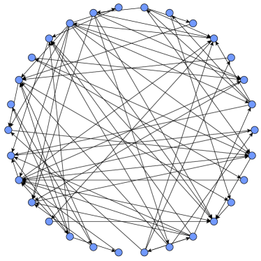
Figure 5: This gene regulatory network contains 30 vertexes which are represented by blue circles. One edge starts at gene 1 and ends at gene 2 if gene 1 has influence on gene 2.

Performance evaluation.

Six commonly-used criteria are considered to measure the performance, i.e., sensitivity (SN), specificity (SP), accuracy (ACC), F-measure, Matthews correlation coefficient (MCC), and the Area Under ROC Curve (AUC):

$$\text{SN}=\frac{\text{TP}}{\text{TP}+\text{FN}},\quad\text{SP}=\frac{\text{TN}}{\text{TN}+\text{FP}},$$

$$\text{ACC}=\frac{\text{TP}+\text{TN}}{\text{TP}+\text{FP}+\text{TN}+\text{FN}},$$

$$\text{F-measure}=\frac{2\times\text{SN}\times\text{SP}}{\text{SN}+\text{SP}},$$

$$\text{MCC}=\frac{\text{TP}\times\text{TN}-\text{FP}\times\text{FN}}{\sqrt{(\text{TP}+\text{FP})(\text{TP}+\text{FN})(\text{TN}+\text{FP})(\text{TN}+\text{FN})}},$$

where TP and TN denote the true positive and true negative, and FP and FN denote the false positive and false negative, respectively. With these criteria, we compare the performance of our method with six representative algorithms, including PCC, ARACNE (Margolin et al., 2006), CLR (Faith et al., 2007), MINET (Meyer et al., 2008), GENIE3 (Huynh-Thu et al., 2010), TIGRESS (Haury et al., 2012). The results are summarized in Table 1. Our method outperforms other six state-of-art methods: the AUC of our method achieve 0.7 higher which is far more than other methods; 5 out of 6 different measure show that our method has significant advantage compared to other algorithms.

	SN	SP	ACC	F-measure	MCC	AUC
Our Method	0.6875$\pm$0.0295	0.7397$\pm$0.0319	0.7119$\pm$0.0305	0.7126$\pm$0.0306	0.4264$\pm$0.0611	0.7136$\pm$0.0306
GENIE3	0.5611$\pm$0.0277	0.4984$\pm$0.0547	0.5319$\pm$0.0244	0.5279$\pm$0.0277	0.0595$\pm$0.0547	0.5662$\pm$0.0244
CLR	0.5167$\pm$0.0583	0.4476$\pm$0.1147	0.4844$\pm$0.0575	0.4795$\pm$0.0583	-0.0357$\pm$0.1147	0.5210$\pm$0.0575
TIGRESS	0.1333$\pm$0.0541	0.8302$\pm$0.0367	0.4585$\pm$0.0374	0.2258$\pm$0.0817	-0.0552$\pm$0.1061	0.5567$\pm$0.0358
PCC	0.5042$\pm$0.0124	0.4333$\pm$0.0245	0.4711$\pm$0.0101	0.4661$\pm$0.0124	-0.0625$\pm$0.0245	0.5091$\pm$0.0101
ARACNE	0.1167$\pm$0.0519	0.9127$\pm$0.0579	0.4881$\pm$0.0197	0.2051$\pm$0.0519	0.0479$\pm$0.0579	0.5808$\pm$0.0197
MINET	0.5764$\pm$0.0425	0.5381$\pm$0.0888	0.5585$\pm$0.0458	0.5547$\pm$0.0425	0.1147$\pm$0.0888	0.5910$\pm$0.0458

Table 1: Performance evaluation of our method and six other state-of-art methods

6 Conclusion

This paper considers the TVCS constrained optimization, motivated by the intrinsic restrictions for many important applications, for example, in bioinformatics, recommendation system, and crowdsourcing. To solve the cardinality constrained problem, the key step is the projection onto the cardinality constraints. Although the projection onto the overlapped cardinality constraints is NP-hard in general, we prove that if the TVCS condition is satisfied the projection can be reduced to a linear programming. We further prove that there is an iterative algorithm which finds an integer solution to the linear programming within time complexity $O((p+|\mathcal{G}|)\log_{\alpha}{1\over R})$, where $R$ is the distance from the initial point to the optimization solution and $\alpha<1$ is the convergence rate. We finally use synthetic experiments and two interesting applications in bioinformatics and crowdsourcing to validate the proposed TVCS model.

In the supplementary materials, we include all the proofs for the proposed theorems and the detailed derivations for the formulation of the crowdsourcing task assignment problem.

1 Proof of Lemma 1

Firstly we show how to convert the projection problem (2) to a support set selection problem. For any vector ${\bf w}$, let vector ${\bf x}\in\{0,1\}^{p}$ indicate the nonzero positions of ${\bf w}$, then we can claim that

$$\|{\bf v}-{\bf v}_{{\bf x}}\|^{2}\leq\|{\bf v}-{\bf w}\|^{2}$$

where ${\bf v}_{{\bf x}}$ is a vector having same dimension with ${\bf v}$, and it keeps elements at positions where ${\bf x}$ has “1”, and fills zeros at positions where ${\bf x}$ has “0”. In addition, vector ${\bf w}\in\Omega(\mathcal{G},{\bf s})$ if and only if its support set indicator vector ${\bf x}$ satisfies $A{\bf x}\leq{\bf s}$, given $A$ is defined in (4).

So the problem (2) can be converted to integer programming:

$$\min_{{\bf x}\in\{0,1\}^{p}}\quad \|{\bf v}-{\bf v}_{{\bf x}}\|^{2}$$ (9)

subject to $$A{\bf x}\leq{\bf s}$$

and the objective can be further simplified:

$$\|{\bf v}-{\bf v}_{{\bf x}}\|^{2} =\langle{\bf v}^{2},{\bf{1}}-{\bf x}\rangle$$

$$=\|{\bf v}\|^{2}-\langle{\bf v}^{2},{\bf x}\rangle$$

Since ${\bf v}$ is constant here, then the problem (9) is equivalent to the ILP (3), which means problem (2) is equivalent to ILP (3). Then we complete the proof.

2 Proof of Theorem 2

To prove Theorem 2, we use the concept of totally unimodular matrix.

Definition 2.

Totally Unimodular (TU) Matrix. An integer matrix is TU, if the determinant of any square submatrices is in the set $\{-1,0,1\}$.

Proposition 1.

If $A$ is TU, then $A^{\top}$ is TU, and their concatenations with identity matrices (i.e. $[A,I],[A^{\top},I]^{\top}$) are still TU.

Proof.

Since transposing matrix will not change the determinant, so it is obvious $A^{\top}$ is TU.
Then we prove stacking with identity matrix $I$ preserves TU property. We prove it by induction. Firstly, we show that submatrix with size 1 always has determinant in $\{-1,0,1\}$, because any element from $I$ is either 1 or 0. Now consider a submatrix with size $k$ having determinant in $\{-1,0,1\}$, then submatrix with size $k+1$ will still have determinant in $\{-1,0,1\}$. To show this, we only need to prove that adding a new row/column from $I$ will not change the determinant out of set $\{-1,0,1\}$. Since any row/column from $I$ only has one nonzero element “1”, we can eliminate other elements in the same position by subtracting a multiple of this row/column to other rows/columns. After that, we can remove this row and column, and the determinant can only change its sign. So we know that submatrix with size $k+1$ has determinant in $\{-1,0,1\}$ if submatrix with size $k$ has determinant in $\{-1,0,1\}$. ∎

Lemma 4.

If $A$ is TU, ${\bf s}$ is an integer vector, then all vertices of the following polytope are integer points:

$$\{{\bf x}\mid A{\bf x}\leq{\bf s},{\bf x}\in[0,1]^{p}\}$$ (10)

Proof.

We can have an equivalent form of this polytope:

$$\left\{{\bf x}\middle|\begin{bmatrix}A\\ I\end{bmatrix}{\bf x}\leq\begin{bmatrix}{\bf s}\\ {\bf{1}}\end{bmatrix},{\bf x}\geq{\bf{0}}\right\}$$ (11)

From Proposition 1, we know that matrix

$$\begin{bmatrix}A\\ I\end{bmatrix}$$

is TU if $A$ is TU, so this meets the case in Theorem 13.2 (see Papadimitriou and Steiglitz, 1982, chap 13). Then we complete the proof. ∎

Lemma 5.

If $C$ is the matrix whose each row is the indicator vector of a group $g\in\mathcal{G}_{1}\cup\mathcal{G}_{2}$ in our TVCS model, then $C$ is a TU matrix.

Proof.

Since $C$’s rows are the indicator vectors of groups in $\mathcal{G}$, so $C_{ij}\in\{0,1\}$. From the definition 1, we know that there are at most two “1”s in each column. For the column which has two “1”s, the two corresponding groups are from $\mathcal{G}_{1}$ and $\mathcal{G}_{2}$ respectively. (Because we know that groups within $\mathcal{G}_{1}$ or $\mathcal{G}_{2}$ do not overlap.)

By this way, our matrix $C$ meets the case in Theorem 13.3 (see Papadimitriou and Steiglitz, 1982, chap 13), and it is a TU matrix. ∎

Lemma 6.

Recall the matrix $A$ in equation (4):

$$A=\begin{bmatrix}{\bf{1}}^{\top}\\ C\end{bmatrix}$$

If it is constructed from the TVCS model, then $A$ is a TU matrix.

Proof.

From Lemma 5, we know $C$ is a TU matrix for any $\mathcal{G}$ of our TVCS model. In other words, any submatrix restricted in $C$ has determinant $-1$, $0$, or $1$. Therefore, we only need to consider the submatrix of $A^{\prime}$ has overlaps with the first row ${\bf{1}}^{\top}$. There are only three possible forms of such submatrix $S$. We will show all of their determinants are in $\{-1,0,1\}$.

1. At least one column of $S$ has a single “$1$”, so it must appear in the first row ${\bf{1}}^{\top}$. By exchanging such column with the last column (which can only influence the sign of determinant), we can transform it with form:

   $$\left[\begin{matrix}{\bf{1}}^{\top}&1\\ \bar{C}&{\bf{0}}\end{matrix}\right]$$

   where $\bar{C}$ is any submatrix of $C$. From the matrix determinant property, we have $|S|=\pm|\bar{C}|\in\{-1,0,1\}$. Therefore, submatrix $S$ in such form have determinants in $\{-1,0,1\}$.

2. All columns of $S$ have three “$1$” elements (the last row has “1” for every column). For the rows which are from $C$, we can sum all the rows to a certain row (this will not change the determinant). By this way we transform $S$ to the following form:

   $$\left[\begin{matrix}{\bf{1}}^{\top}\\ {\bf 2}^{\top}\\ \bar{C}\end{matrix}\right]$$

   where $\bar{C}$ is a submatrix of $C$. In this case, $S$ is not full rank, so its determinant is 0.

3. Each column in $S$ contains at least two “$1$” elements, and there exists one column which has exactly two “$1$”s. By exchanging it to the last column, we can transform it to be:

   $$\left[\begin{matrix}{\bf{1}}^{\top}&1\\ \cdots&{\bf{0}}\\ \bar{C}_{i}&1\\ \cdots&{\bf{0}}\end{matrix}\right]$$

   This means that one “1” is in the first row, and another is in the row from $C$, let us say it’s $\bar{C}_{i}$. Since subtracting one row from another row will not change the determinant, we can let the first row subtract $\bar{C}_{i}$:

   $$\left[\begin{matrix}{\bf{1}}^{\top}&1\\ \cdots&{\bf{0}}\\ \bar{C}_{i}&1\\ \cdots&{\bf{0}}\end{matrix}\right]\rightarrow\left[\begin{matrix}{\bf{1}}^{\top}-\bar{C}_{i}&0\\ \cdots&{\bf{0}}\\ \bar{C}_{i}&1\\ \cdots&{\bf{0}}\end{matrix}\right]$$

   Now the last column only has a single “1” in the $i$-th row. We can generate a smaller matrix $S^{\prime}$ by removing the $i$-th row and the last column, and if $S^{\prime}$ has determinant in $\{-1,0,1\}$, so does $S$.

   $$\left[\begin{matrix}{\bf{1}}^{\top}-\bar{C}_{i}&0\\ \cdots&{\bf{0}}\\ \bar{C}_{i}&1\\ \cdots&{\bf{0}}\end{matrix}\right]\rightarrow S^{\prime}=\left[\begin{matrix}{\bf{1}}^{\top}-\bar{C}_{i}\\ \cdots\\ \cdots\end{matrix}\right]$$

   If $\bar{C}_{i}\neq{\bf{0}}^{\top}$, then there are some positions (including $j$-th column) in the first row will become zeros. For any column of matrix $S^{\prime}$ which has “0” element in the first row, there are two cases:

   1. This column only contains zeros, i.e. $S^{\prime}$ has zero determinant.

   2. This column contains a single “1”, we can generate a smaller matrix $S^{\prime\prime}$ by removing this column and the row where this “1” sits. If $S^{\prime\prime}$ has determinant in $\{-1,0,1\}$, so does $S^{\prime}$.

   Notice that it is impossible for the case that such column has two “1”s. (Since each column can have at most three “1”s, and we already remove the “1” in the first row by subtraction, and discard another “1” by removing $\bar{C}_{i}$.) In the above case (b), we can repeat removing columns and rows until we get a degenerate matrix (has 0 determinant), or a matrix whose first row does not have zeros. For the later situation, we can process it by same procedures as the original matrix $S$ unless it only has one row and one column, i.e. a matrix having single element “1” (has determinant 1).

   If $\bar{C}_{i}={\bf{0}}^{\top}$, we can also process it by same procedures as the original matrix $S$.

Therefore, we have proved that any square submatrix $S$ in $A^{\prime}$ has determinant in $\{-1,0,1\}$, which means $A^{\prime}$ is TU, and hence $A$ is TU. ∎

Applying Lemma 4 and Lemma 6, we complete the proof of Theorem 2.

3 Proof of Theorem 3

To prove Theorem 3, we start with several lemmas.

Lemma 7.

Formulate the feasibility problem as problem (7), let $f$ be the objective of the formulation in Theorem 3. If $f^{*}=0$, there exists a $\lambda$ such that

$$f({\bf z})-f^{*}\geq\frac{\lambda}{2}\|{\bf z}-P_{{\bf z}^{*}}({\bf z})\|^{2},\forall{\bf z}\in\Omega$$

where $P_{{\bf z}^{*}}({\bf z})$ is the optimal point which is closet to ${\bf z}$.

Proof.

Since $f^{*}=0$, there exists at least an ${\bf z}^{*}$ such that

$$A{\bf z}^{*}-a\leq 0$$

$$B{\bf z}^{*}=b$$

$$C{\bf z}^{*}\leq c$$

From Hoffman’s Theorem (Hoffman, 2003), we know that there exists a $\lambda>0$, such that

$$\frac{\lambda}{2}\|{\bf z}-P_{{\bf z}^{*}}({\bf z})\|^{2}\leq\|[A{\bf z}-a]_{+}\|^{2}+\|B{\bf z}-b\|^{2}+\|[C{\bf z}-c]_{+}\|^{2}$$

Therefore, we know for any ${\bf z}$ in $\Omega$,

$$C{\bf z}\leq c$$

and

$$\frac{\lambda}{2}\|{\bf z}-P_{{\bf z}^{*}}({\bf z})\|^{2}\leq\|[A{\bf z}-a]_{+}\|^{2}+\|B{\bf z}-b\|^{2}$$

∎

Using the lemma above, we can prove the Theorem 3 now.

Proof.

Denote by $\Delta_{t}:=\|{\bf z}^{t}-P_{{\bf z}^{*}}({\bf z}^{t})\|^{2}$. We have

$$\Delta_{t+1} =\|{\bf z}^{t+1}-P_{{\bf z}^{*}}({\bf z}^{t+1})\|^{2}$$

$$\leq\|{\bf z}^{t+1}-P_{{\bf z}^{*}}({\bf z}^{t})\|^{2}$$

$$\leq\|{\bf z}^{t}-P_{{\bf z}^{*}}({\bf z}^{t})+{\bf z}^{t+1}-{\bf z}^{t}\|^{2}$$

$$=\|{\bf z}^{t}-P_{{\bf z}^{*}}({\bf z}^{t})\|^{2}+\|{\bf z}^{t+1}-{\bf z}_{t}\|^{2}+2\langle{\bf z}^{t+1}-{\bf z}^{t},{\bf z}^{t}-P_{{\bf z}^{*}}({\bf z}^{t})\rangle$$

$$=\Delta_{t}-\|{\bf z}^{t+1}-{\bf z}^{t}\|^{2}+2\langle{\bf z}^{t+1}-{\bf z}^{t},{\bf z}^{t+1}-P_{{\bf z}^{*}}({\bf z}^{t})\rangle$$

$$\leq\Delta_{t}-\|{\bf z}^{t+1}-{\bf z}^{t}\|^{2}-2\gamma\langle\nabla f({\bf z}^{t}),{\bf z}^{t+1}-P_{{\bf z}^{*}}({\bf z}^{t})\rangle$$

Let $T=\langle\nabla f({\bf z}^{t}),{\bf z}^{t+1}-P_{{\bf z}^{*}}({\bf z}^{t})\rangle$. Then we have

$$T =\langle\nabla f({\bf z}^{t}),{\bf z}^{t+1}-P_{{\bf z}^{*}}({\bf z}^{t})\rangle$$

$$=\langle\nabla f({\bf z}^{t}),{\bf z}^{t}-P_{{\bf z}^{*}}({\bf z}^{t})\rangle+\langle\nabla f({\bf z}^{t}),{\bf z}^{t+1}-{\bf z}^{t}\rangle$$

$$\geq-f^{*}+f({\bf z}^{t})+f({\bf z}^{t+1})-f({\bf z}^{t})-\frac{L}{2}\|{\bf z}^{t+1}-{\bf z}^{t}\|^{2}$$

$$=f({\bf z}^{t+1})-f^{*}-\frac{L}{2}\|{\bf z}^{t+1}-{\bf z}^{t}\|^{2}$$

where $L$ is the Lipschitz continuous gradient constant. Back to the original inequality, we have

$$\|{\bf z}^{t+1}-P_{{\bf z}^{*}}({\bf z}^{t+1})\|^{2} \leq\Delta_{t}-\|{\bf z}^{t+1}-{\bf z}^{t}\|^{2}-2\gamma\langle\nabla f({\bf z}^{t}),{\bf z}^{t+1}-P_{{\bf z}^{*}}({\bf z}^{t})\rangle$$

$$\leq\Delta_{t}-(1-L\gamma)\|{\bf z}^{t+1}-{\bf z}^{t}\|^{2}-2\gamma(f({\bf z}^{t+1})-f^{*})$$

$$\leq\Delta_{t}-(1-L\gamma)\|{\bf z}^{t+1}-{\bf z}^{t}\|^{2}-2\gamma\frac{\lambda}{2}\|{\bf z}^{t+1}-P_{{\bf z}^{*}}({\bf z}^{t+1})\|^{2}$$

where the last inequality comes from Lemma 7.

Let $\gamma=\frac{1}{L}$ and we have

$$(1+\frac{\lambda}{L})\Delta_{t+1} \leq\Delta_{t}$$

$$\Delta_{t+1} \leq\frac{1}{1+\frac{\lambda}{L}}\Delta_{t}$$

which shows the linear convergence rate $\alpha=\frac{1}{1+\frac{\lambda}{L}}$, then it completes the proof. ∎

4 Formulation of the Expected Accuracy in Crowdsourcing Task Assignment

In crowdsourcing task assignment problem, recall the objective function of problem (8):

$${1\over m}\sum_{j=1}^{m}\mathcal{E}_{\text{acc}}(Q_{\cdot,j},X_{\cdot,j})$$

For the $j$-th task, $\mathcal{E}_{\text{acc}}(Q_{\cdot,j},X_{\cdot,j})$ is defined in the following:

$$\mathcal{E}_{\text{acc}}(Q_{\cdot,j},X_{\cdot,j})= \mathbb{P}(\hat{{\bf y}}_{j}=1|{\bf y}_{j}=1)\mathbb{P}({\bf y}_{j}=1)+\mathbb{P}(\hat{{\bf y}}_{j}=0|{\bf y}_{j}=0)\mathbb{P}({\bf y}_{j}=0)$$

$$= \mathbb{E}_{\hat{Y}_{\Omega_{j},j}|{\bf y}_{j}=1}[{\bf I}(\hat{{\bf y}}_{j}=1)]\mathbb{P}({\bf y}_{j}=1)+\mathbb{E}_{\hat{Y}_{\Omega_{j},j}|{\bf y}_{j}=0}[{\bf I}(\hat{{\bf y}}_{j}=0)]\mathbb{P}({\bf y}_{j}=0)$$ (12)

where ${\bf I}(\cdot)$ is the indicator function. We can further specify this formulation by considering the equivalent forms for $\hat{{\bf y}}_{j}=1$ and $\hat{{\bf y}}_{j}=0$:

$$\hat{{\bf y}}_{j}=1$$

$$\Leftrightarrow \mathbb{P}({\bf y}_{j}=1|\hat{Y}_{\Omega_{j},j})\geq\mathbb{P}({\bf y}_{j}=0|\hat{Y}_{\Omega_{j},j})$$

$$\Leftrightarrow {\mathbb{P}(\hat{Y}_{\Omega_{j},j}|{\bf y}_{j}=1)\over\mathbb{P}(\hat{Y}_{\Omega_{j},j}|{\bf y}_{j}=0)}\geq{\mathbb{P}({\bf y}_{j}=0)\over\mathbb{P}({\bf y}_{j}=1)}$$

$$\Leftrightarrow \prod_{i\in\Omega_{j}}\left({Q_{ij}\over 1-Q_{ij}}\right)^{2\hat{Y}_{i,j}-1}\geq{\mathbb{P}({\bf y}_{j}=0)\over\mathbb{P}({\bf y}_{j}=1)}$$

$$\Leftrightarrow \sum_{i\in\Omega_{j}}(2\hat{Y}_{i,j}-1)\log\left({Q_{ij}\over 1-Q_{ij}}\right)\geq\log\left({\mathbb{P}({\bf y}_{j}=0)\over\mathbb{P}({\bf y}_{j}=1)}\right)$$

$$\Leftrightarrow \sum_{i=1}^{n}X_{ij}(2\hat{Y}_{i,j}-1)\log\left({Q_{ij}\over 1-Q_{ij}}\right)-\log\left({\mathbb{P}({\bf y}_{j}=0)\over\mathbb{P}({\bf y}_{j}=1)}\right)\geq 0$$

Similar derivation can be applied to $\hat{{\bf y}}_{j}=0$ (change “$\geq$” to “$<$”). Here we substitute the indicator function ${\bf I}(t\geq 0)$ as sigmoid function $S(t)={1\over 1+\exp(-t)}$ to obtain a smooth approximation. Denote by $Z_{ij}:=(2\hat{Y}_{i,j}-1)\log\left({Q_{ij}/(1-Q_{ij}})\right)$ and ${\bf r}_{j}:=\log\left({\mathbb{P}({\bf y}_{j}=0)/\mathbb{P}({\bf y}_{j}=1)}\right)$ for short. The (smooth) objective turns out to be:

$${1\over m}\sum_{j=1}^{m}\Bigg{(}\mathbb{E}_{\hat{Y}|{\bf y}_{j}=1}\left[S\left(\sum_{i=1}^{n}Z_{ij}X_{ij}-{\bf r}_{j}\right)\right]\mathbb{P}({\bf y}_{j}=1)+\mathbb{E}_{\hat{Y}|{\bf y}_{j}=0}\left[S\left({\bf r}_{j}-\sum_{i=1}^{n}Z_{ij}X_{ij}\right)\right]\mathbb{P}({\bf y}_{j}=0)\Bigg{)}$$

and its stochastic gradient is:

$${\bf g}(X)_{\cdot,j}= {1\over m}\mathbb{P}({\bf y}_{j}=1)(1-S(\sum_{i=1}^{n}Z_{ij}^{{\bf y}_{j}=1}X_{ij}-{\bf r}_{j}))S(\sum_{i=1}^{n}Z_{ij}^{{\bf y}_{j}=1}X_{ij}-{\bf r}_{j})Z_{\cdot,j}^{{\bf y}_{j}=1}+$$

$${1\over m}\mathbb{P}({\bf y}_{j}=0)(1-S(\sum_{i=1}^{n}Z_{ij}^{{\bf y}_{j}=0}X_{ij}-{\bf r}_{j}))S(\sum_{i=1}^{n}Z_{ij}^{{\bf y}_{j}=0}X_{ij}-{\bf r}_{j})Z_{\cdot,j}^{{\bf y}_{j}=0}$$

where $Z^{{\bf y}_{j}=1}$ (or $Z^{{\bf y}_{j}=0}$) is generated by sampling $\hat{Y}$ given ${\bf y}_{j}=1$ (or ${\bf y}_{j}=0$).

References

- Bach et al. [2012] F. Bach, R. Jenatton, J. Mairal, G. Obozinski, et al. Structured sparsity through convex optimization. Statistical Science, 27(4):450–468, 2012.
- Baraniuk et al. [2010] R. G. Baraniuk, V. Cevher, M. F. Duarte, and C. Hegde. Model-based compressive sensing. Information Theory, IEEE Transactions on, 56(4):1982–2001, 2010.
- Candes et al. [2006] E. J. Candes, J. K. Romberg, and T. Tao. Stable signal recovery from incomplete and inaccurate measurements. Communications on pure and applied mathematics, 59(8):1207–1223, 2006.
- Cevher et al. [2009] V. Cevher, P. Indyk, C. Hegde, and R. G. Baraniuk. Recovery of clustered sparse signals from compressive measurements. Technical report, DTIC Document, 2009.
- El Halabi and Cevher [2015] M. El Halabi and V. Cevher. A totally unimodular view of structured sparsity. In Proceedings of the Eighteenth International Conference on Artificial Intelligence and Statistics, pages 223–231, 2015.
- Faith et al. [2007] J. J. Faith, B. Hayete, J. T. Thaden, I. Mogno, J. Wierzbowski, G. Cottarel, S. Kasif, J. J. Collins, and T. S. Gardner. Large-scale mapping and validation of escherichia coli transcriptional regulation from a compendium of expression profiles. PLoS biol, 5(1):e8, 2007.
- Haury et al. [2012] A.-C. Haury, F. Mordelet, P. Vera-Licona, and J.-P. Vert. Tigress: trustful inference of gene regulation using stability selection. BMC systems biology, 6(1):145, 2012.
- Hegde et al. [2009] C. Hegde, M. F. Duarte, and V. Cevher. Compressive sensing recovery of spike trains using a structured sparsity model. In SPARS’09-Signal Processing with Adaptive Sparse Structured Representations, 2009.
- Hegde et al. [2015a] C. Hegde, P. Indyk, and L. Schmidt. Approximation algorithms for model-based compressive sensing. Information Theory, IEEE Transactions on, 61(9):5129–5147, 2015a.
- Hegde et al. [2015b] C. Hegde, P. Indyk, and L. Schmidt. A nearly-linear time framework for graph-structured sparsity. In Proceedings of the 32nd International Conference on Machine Learning (ICML-15), pages 928–937, 2015b.
- Ho et al. [2013] C.-J. Ho, S. Jabbari, and J. W. Vaughan. Adaptive task assignment for crowdsourced classification. In Proceedings of The 30th International Conference on Machine Learning, pages 534–542, 2013.
- Hoffman [2003] A. J. Hoffman. On approximate solutions of systems of linear inequalities. In Selected Papers Of Alan J Hoffman: With Commentary, pages 174–176. 2003.
- Huynh-Thu et al. [2010] V. A. Huynh-Thu, A. Irrthum, L. Wehenkel, and P. Geurts. Inferring regulatory networks from expression data using tree-based methods. PloS one, 5(9):e12776, 2010.
- Jenatton et al. [2011] R. Jenatton, J. Mairal, G. Obozinski, and F. Bach. Proximal methods for hierarchical sparse coding. Journal of Machine Learning Research, 12(Jul):2297–2334, 2011.
- Kong et al. [2014] D. Kong, R. Fujimaki, J. Liu, F. Nie, and C. Ding. Exclusive feature learning on arbitrary structures via -norm. In Advances in Neural Information Processing Systems, pages 1655–1663, 2014.
- Liu and Wright [2015] J. Liu and S. J. Wright. Asynchronous stochastic coordinate descent: Parallelism and convergence properties. SIAM Journal on Optimization, 25(1):351–376, 2015.
- Marbach et al. [2009] D. Marbach, T. Schaffter, C. Mattiussi, and D. Floreano. Generating realistic in silico gene networks for performance assessment of reverse engineering methods. Journal of computational biology, 16(2):229–239, 2009.
- Margolin et al. [2006] A. A. Margolin, I. Nemenman, K. Basso, C. Wiggins, G. Stolovitzky, R. D. Favera, and A. Califano. Aracne: an algorithm for the reconstruction of gene regulatory networks in a mammalian cellular context. BMC bioinformatics, 7(Suppl 1):S7, 2006.
- Meyer et al. [2008] P. E. Meyer, F. Lafitte, and G. Bontempi. minet: Ar/bioconductor package for inferring large transcriptional networks using mutual information. BMC bioinformatics, 9(1):461, 2008.
- Needell and Tropp [2009] D. Needell and J. A. Tropp. Cosamp: Iterative signal recovery from incomplete and inaccurate samples. Applied and Computational Harmonic Analysis, 26(3):301–321, 2009.
- Nguyen et al. [2012] N. Nguyen, S. Chin, and T. D. Tran. A unified iterative greedy algorithm for sparsity constrained optimization. 2012.
- Nguyen et al. [2014] N. Nguyen, D. Needell, and T. Woolf. Linear convergence of stochastic iterative greedy algorithms with sparse constraints. arXiv preprint arXiv:1407.0088, 2014.
- Olshausen and Field [1997] B. A. Olshausen and D. J. Field. Sparse coding with an overcomplete basis set: A strategy employed by v1? Vision research, 37(23):3311–3325, 1997.
- Papadimitriou and Steiglitz [1982] C. H. Papadimitriou and K. Steiglitz. Combinatorial optimization: algorithms and complexity. Courier Corporation, 1982.
- Schaffter et al. [2011] T. Schaffter, D. Marbach, and D. Floreano. Genenetweaver: in silico benchmark generation and performance profiling of network inference methods. Bioinformatics, 27(16):2263–2270, 2011.
- Yang et al. [2016] H. Yang, Y. Huang, L. Tran, J. Liu, and S. Huang. On benefits of selection diversity via bilevel exclusive sparsity. In Computer Vision and Pattern Recognition (CVPR), 2016 IEEE Conference on. IEEE, 2016.
- Yuan and Lin [2006] M. Yuan and Y. Lin. Model selection and estimation in regression with grouped variables. Journal of the Royal Statistical Society: Series B (Statistical Methodology), 68(1):49–67, 2006.
- Yuan et al. [2014] X. Yuan, P. Li, and T. Zhang. Gradient hard thresholding pursuit for sparsity-constrained optimization. In Proceedings of The 31st International Conference on Machine Learning, pages 127–135, 2014.
- Yuan et al. [2016] X. Yuan, P. Li, and T. Zhang. Exact recovery of hard thresholding pursuit. In Advances in Neural Information Processing Systems, pages 3558–3566, 2016.
- Zhang [2009] T. Zhang. On the consistency of feature selection using greedy least squares regression. Journal of Machine Learning Research, 10(Mar):555–568, 2009.
- Zhou et al. [2010] Y. Zhou, R. Jin, and S. C. Hoi. Exclusive lasso for multi-task feature selection. In AISTATS, volume 9, pages 988–995, 2010.
- Zou and Conzen [2005] M. Zou and S. D. Conzen. A new dynamic bayesian network (dbn) approach for identifying gene regulatory networks from time course microarray data. Bioinformatics, 21(1):71–79, 2005.
Supplementary Material