Gaussian-Mixture-Model-based Cluster Analysis Finds Five Kinds of Gamma Ray Bursts in the BATSE Catalog

Abstract

Clustering methods are an important tool to enumerate and describe the different coherent kinds of Gamma Ray Bursts (GRBs). But their performance can be affected by a number of factors such as the choice of clustering algorithm and inherent associated assumptions, the inclusion of variables in clustering, nature of initialization methods used or the iterative algorithm or the criterion used to judge the optimal number of groups supported by the data. We analyzed GRBs from the BATSE 4Br catalog using $k$-means and Gaussian Mixture Models-based clustering methods and found that after accounting for all the above factors, all six variables – different subsets of which have been used in the literature – and that are, namely, the flux duration variables ($T_{50}$, $T_{90}$), the peak flux ($P_{256}$) measured in 256-millisecond bins, the total fluence ($F_{t}$) and the spectral hardness ratios ($H_{32}$ and $H_{321}$) contain information on clustering. Further, our analysis found evidence of five different kinds of GRBs and that these groups have different kinds of dispersions in terms of shape, size and orientation. In terms of duration, fluence and spectrum, the five types of GRBs were characterized as intermediate/faint/intermediate, long/intermediate/soft, intermediate/intermediate/intermediate, short/faint/hard and long/bright/intermediate.

1 Introduction

Gamma Ray Bursts (GRBs) are the brightest known electromagnetic events known to occur in space and have been studied extensively ever since their discovery in the late sixties. While the cosmological origin of GRBs is well-established, questions on their source and nature remain unresolved (Chattopadhyay et al., 2007; Piran, 2005). Indeed, as explained by Shahmoradi & Nemiroff (2015), researchers (e.g., Mazets et al., 1981; Norris et al., 1984; Dezalay et al., 1992) have hypothesized that GRBs really belong to a heterogeneous group with several sub-populations, but the exact number and descriptive properties of these groups is an area of active research and investigation. Most analyses have traditionally focused on univariate statistical and descriptive methods for classification, with particular focus on the duration of GRBs (as measured by $\log_{10}T_{90}$ or the time within which 90% of the GRB flux has arrived ). For example, Kouveliotou et al. (1993) analyzed the $\log_{10}T_{90}$ distribution of 222 GRBs of the Burst and Transient Source Experiment (BATSE) 1B Catalog and found it to have a bimodal distribution. This led to the establishment of the well-known classification of GRBs into the two classes, one of short bursts (of durations less than 2s) and the other class of long bursts (bursts with durations greater than 2s). Pendleton et al. (1997) applied spectral analysis technique to $882$ BATSE GRBs and provided evidence about the existence of bursts populations of two types, the HE (High Energy) bursts and the NHE (no-High Energy) bursts. The progenitors of long GRBs have mainly been associated with the collapse of massive stars (Paczyński, 1998; Woosley & Bloom, 2006) while those of short GRBs are thought to be NS-NS, that is the merger of two neutron stars, or NS-BH, that is the merger of a neutron star with a black hole (Nakar, 2007). Horváth (1998) made both two- and three-Gaussian fits to the $\log_{10}T_{90}$ variable of the 797 GRBs in the BATSE 3B Catalog and indicated the presence of a third Gaussian component at a 99.98% level of significance thus providing evidence of a third class(see also Horváth, 2002). Similar findings were also reported on the distribution of $T_{90}$ with the BeppoSAX (Horváth, 2009), Swift/BAT (Horváth et al., 2008) and Fermi/GBM (Tarnopolski, 2015) datasets, with the observation holding regardless of whether ${\chi}^{2}$-fitting (Horváth, 1998; Tarnopolski, 2015) or maximum likelihood (Horváth, 2002; Horváth et al., 2008; Horváth, 2009; Horváth & Tóth, 2016) was used in analysis. Zitouni et al. (2015) analyzed 248 Swift/BAT GRBs with known redshifts and confirmed a preference of statistical tests for three groups instead of two. More recently however, Zhang et al. (2016) and Kulkarni & Desai (2017) studied the duration distributions of the BATSE, Swift and Fermi GRB datasets and concluded that only the Swift dataset potentially supports a three-Gaussians model, while two-Gaussians models are strongly supported by the BATSE and Fermi datasets. Three kinds of GRBs were also found in the Swift GRB datasets by de Ugarte Postigo et al. (2011) and Horváth & Tóth (2016).

Mukherjee et al. (1998) explain that many studies in astronomy have typically only used univariate and bivariate statistical analyses, potentially providing an incomplete understanding of the relationships between the different variables in the GRB datasets. Building on the review of multivariate statistical methods provided by Feigelson & Babu (1998) for the benefit of more thorough analysis of datasets in astronomy, Mukherjee et al. (1998) used both non-parametric hierarchical clustering and a more formal Model-based Clustering (MBC) approach (with Gaussian mixtures and using six and three parameters) on 797 BATSE 3B catalog GRBs and found evidence in favour of three groups. Chattopadhyay et al. (2007) carried out clustering using the $k$-means algorithm and MBC with Dirichlet Process mixture modeling on the larger BATSE 4B catalog (as per a reviewer of this article) of 1594 GRBs using the six variables used by Mukherjee et al. (1998) and supported the presence of a third group. Similar findings were reported by Veres et al. (2010) and Horváth et al. (2010), but their analysis used the smaller Swift/BAT dataset and just two variables (i.e. $\log_{10}T_{90}$ and the log-hardness ratio $\log_{10}H_{32}$ where $H_{32}=F_{2}/F_{3}$, with $F_{2}$ and $F_{3}$ being the time-integrated fluences in the 50-100 keV and 100-300 keV spectral channels, respectively). Horváth et al. (2010) also argued lack of significant evidence for a fourth cluster by means of a likelihood ratio $\chi^{2}$-test on twice the difference in loglikelihood for three and four clusters. (Note, however, that the use of the $\chi^{2}$ test on twice the difference in loglikelihoods between two models assumes that the larger model is nested within the null model, an assumption that does not generally hold for MBC or other non-hierarchical clustering algorithms). Our own experiments using $k$-means and the Jump statistic (Sugar & James, 2003) with the BATSE GRB dataset and variables used by Chattopadhyay et al. (2007) did not replicate their results. This led us to review and perform a detailed investigation and cluster analysis of the GRBs in the BATSE 4Br catalog.

Cluster analysis (Kettenring, 2006; Xu & Wunsch, 2009; Everitt, 2011) is widely used in many disciplines to group observations into homogeneous classes or clusters. Clustering is an unsupervised learning approach wherein classification rules are obtained in the absence of a response variable. As such, it is a difficult problem in general (Maitra, 2001). Many clustering algorithms exist but they can all be broadly grouped into the hierarchical and the non-hierarchical kinds. The first case comprises both agglomerative and divisive clustering algorithms where groups of observations are formed in a tree-like hierarchy with the property that observations that are together at one level are also together higher up the tree. These algorithms typically have criteria set to measure the discrepancy between two entities and also to specify how these distances change upon merging between any two sub-groups. As pointed out by Chattopadhyay et al. (2007), the assumption of a hierarchy is restrictive and such a scheme is methodologically unable to recover or repair from a partitioning happening higher up in the tree.

Non-hierarchical partitional algorithms, on the other hand, lack the regimented structure of their hierarchical counterparts and usually rely on optimizing an objective function, which in the case of MBC, is the observed loglikelihood function given the observations. For a specified number of groups, the optimization problem is typically multimodal and solved by iterative greedy algorithms, therefore careful initialization is important. Various approaches (see e.g. Akaike, 1973, 1974; Schwarz, 1978; Rousseeuw, 1987; Sugar & James, 2003; Maitra et al., 2012) exist to determine the number of homogeneous groups supported by the data.

Even within non-hierarchical clustering, the choice of algorithm (e.g. $k$-means or MBC) is important and hinges on the types and reasonableness of assumptions that underlie the different kinds of groups. For instance, the $k$-means algorithm assumes homogeneous spherically-dispersed groups of roughly similar sizes while MBC allows for greater flexibility in the shapes, orientations and volumes as well as different sizes in the distributions of each group. Another aspect which assumes tremendous significance in the context of all the different studies published using different numbers and sets of variables in the astronomy literature (Mukherjee et al., 1998; Veres et al., 2010; Horváth et al., 2006; Horváth et al., 2010; de Ugarte Postigo et al., 2011; Horváth & Tóth, 2016; Zhang et al., 2016, e.g.), is that of the specific parameters (variables in statistics jargon) that should be used in clustering. Actually, incorporating redundant information by including variables that do not add to clustering information can potentially impact and even give rise to spurious cluster assignments (refer to Raftery & Dean, 2006; Maugis et al., 2009; Witten & Tibshirani, 2010, for both illustrations and potential solutions in different contexts.), Thus, selection of the most relevant variables having discriminating information is very important in the context of clustering.

This paper is organized in three further sections. Section 2 provides an overview of partitional clustering algorithms and discusses issues arising from improper or inadequate initialization, methods for choosing the number of groups and for finding the most relevant variables for inclusion for clustering. GRBs in the BATSE 4Br catalog are clustered and analyzed using these methods in Section 3. The paper concludes with some discussion. Additionally, an online supplement provides the interested reader with commented R (R Core Team, 2016) and (where appropriate, html code) for performing our cluster analysis.

2 Overview of Clustering Methods

We first briefly but comprehensively discuss the many issues bedeviling cluster analysis, especially in the context of GRBs, and strategies to combat them. As mentioned in Section 1, there is a large amount of literature on clustering, so here we focus on issues in methods that are commonly used in astronomy and that are easily implemented using the open-source statistical software R (R Core Team, 2016) and its packages. We restrict attention only to the non-hierarchical $k$-means and MBC algorithms given hierarchical clustering’s inflexibility in allowing for wider classes of models (Chattopadhyay et al., 2007).

2.1 The $k$-means clustering algorithm

Given $n$ $p$-dimensional observations $\boldsymbol{x}_{1},\boldsymbol{x}_{2},\ldots,\boldsymbol{x}_{n}$, the $k$-means algorithm (MacQueen, 1967) groups the observations into a pre-determined ($K$) number of groups $\mathcal{G}_{1},\mathcal{G}_{2},\ldots,\mathcal{G}_{K}$ by minimizing the objective function

$$W_{K}=\sum_{k=1}^{K}\sum_{i=1}^{n}\zeta_{ik}^{(K)}\|\boldsymbol{x}_{i}-\mn@boldsymbol{\mu}_{k}\|^{2},$$ (1)

where $\|\boldsymbol{x}\|=\sqrt{\boldsymbol{x}^{T}\boldsymbol{x}}$ and, for each $i=1,2,\ldots,n$ and $k=1,2,\ldots,K$, we have that $\zeta_{ik}^{(K)}$ is 1 if $\boldsymbol{x}_{i}$ belongs to the $k$th group $\mathcal{G}_{k}$ and is 0 otherwise. In this problem, $\zeta_{ik}^{(K)}$s and $\mn@boldsymbol{\mu}_{k}$s are all statistical parameters over which $W_{K}$ is optimized. Optimizing (1) is an NP-hard problem (Garey & Johnson, 1979) with an iterative solution provided by the $k$-means algorithm (Lloyd, 1982; Forgy, 1965) having the following steps:

1. Initialization. Select $K$ initial seeds for $\mn@boldsymbol{\mu}^{\circ}_{1},\mn@boldsymbol{\mu}^{\circ}_{2},\ldots,\mn@boldsymbol{\mu}^{\circ}_{K}$.

2. Assignment. Assign each observation to the $\boldsymbol{\mu}_{k}^{\circ}$ closest to it. That is, assign $\boldsymbol{x}_{i}$ to $\mathcal{G}_{k}$ where $k=\operatorname*{arg\,min}_{l}\|\boldsymbol{x}_{i}-\boldsymbol{\mu}^{\circ}_{l}\|$. Set $\zeta_{ik}^{(K)}=1$ for when $\boldsymbol{x}_{i}\in\mathcal{G}_{k}$ and 0 otherwise.

3. Parameter updates. Update $\boldsymbol{\mu}^{\circ}_{k}$ to the respective group means. That is, update $\boldsymbol{\mu}^{\circ}_{k}=\sum_{i=1}^{n}\zeta_{ik}^{(K)}\boldsymbol{x}_{i}/\sum_{i=1}^{n}\zeta_{ik}^{(K)}$.

4. Iteration and Convergence. Repeat Steps 2 and 3 until no further rearrangement is possible.

The above $k$-means algorithm is easily described and commonly used, but the statistics community and software use a more efficient variant of the algorithm due to Hartigan & Wong (1979) which keeps track of observations having no possibility of changing immediately, and takes them out of contention from the current update calculations. The R function kmeans() implements this variant as its default.

An important aspect of the $k$-means algorithm is that it treats contributions from each variable uniformly: thus variables with smaller magnitudes would tend to be swamped out by the variables having higher magnitudes in the calculation of Equation (1). Therefore, unless all variables are known to be on the same scale, it is customary for the variables to be scaled individually before optimization.

The $k$-means algorithm needs specification of $K$ to proceed. There are several approaches to determining an optimal $K$, but a quick method that we have also found to work well with $k$-means is the jump statistic (Sugar & James, 2003) that was also used by Chattopadhyay et al. (2007) in their $k$-means clustering of the BATSE 4B GRBs. Given a clustering solution with $K$ groups, the jump statistic involves computing an overall minimum distance measure ($d_{K}$) which is estimated by the distortion $d_{K}^{\prime}$ that, in the $k$-means scenario, can be taken to be the optimized value of (1), that is $d_{K}^{\prime}\equiv W_{K}$. Sugar & James (2003) contend that the distortion curve obtained by plotting $d_{K}^{\prime}$ against $K$ will monotonically decrease with increasing $K$ until $K$ is greater than the true number of groups, after which the curve will level off with a smaller slope. The jump statistic defined by Sugar & James (2003) is defined as $J_{K}=d_{K}^{\prime-Y}-d^{\prime-Y}_{K-1}$. For $K=1$, $J_{K}=d_{K}^{\prime-Y}$. The value of $K$ which gives the largest jump statistic yields the $K$ most supported by the data. The exact choice of $Y$ is left to the user, with no clear guideline but the choice of $Y=p/2$ was used in their experiments, and also adopted by Chattopadhyay et al. (2007) in their GRB analysis. A significance-based bootstrap approach that estimates the $p$-value of a more complicated (higher $K$) solution than needed for describing the data was suggested by Maitra et al. (2012). This method provides $p$-values for solutions with all possible pairs of $K$ and $K^{\prime}>K$ being tested and has the added advantage of even assessing the case of no clustering.

2.2 Model-based clustering

One drawback of $k$-means clustering is that it is an optimization algorithm with no grounding in variability or the mechanism that generated the data (see however, Celeux & Govaert 1992 for writing $k$-means as a Classification-EM algorithm in the context of a GMM and Maitra & Ramler, 2009; Maitra et al., 2012, for framing $k$-means in a nonparametric distributional setting). Model-based clustering (Fraley & Raftery, 2002; Melnykov & Maitra, 2010) provides a principled approach to the problem of clustering by postulating that, for a given total number of components $K$, the observations $\boldsymbol{x}_{1},\boldsymbol{x}_{2},\ldots,\boldsymbol{x}_{n}$ are realizations from the mixture model (McLachlan & Peel, 2000) with density

$$f(x;\nu)=\sum_{k=1}^{\textit{K}}\pi_{k}f_{k}(\boldsymbol{x};\boldsymbol{\nu}_{k})$$ (2)

where $f_{k}(\boldsymbol{x};\boldsymbol{\nu}_{k})$ represents the density of the $k$th group parameterized by $\boldsymbol{\nu}_{k}$ and $\pi_{k}$ represents the mixing proportion of the $k$th group, that is, $\pi_{k}=Pr[\boldsymbol{x}_{i}\in\mathcal{G}_{k}]$ for $k=1,2,\ldots,K$ and $\sum_{k=1}^{K}\pi_{k}=1$. The most commonly-used mixture model is the Gaussian mixture model (GMM), where each $f_{k}(\boldsymbol{x};\boldsymbol{\nu}_{k})$ is taken to be the multivariate Gaussian density $\phi(\boldsymbol{x};\mn@boldsymbol{\mu}_{k},\boldsymbol{\Sigma}_{k})$ with mean $\mn@boldsymbol{\mu}_{k}$ and dispersion matrix $\boldsymbol{\Sigma}_{k}$. Estimation is via the Expectation-Maximization (EM) algorithm Dempster et al. (1977); McLachlan & Krishnan (2008) which has the following steps:

1. Initialization. Obtain starting values $\{(\boldsymbol{\Sigma}_{k}^{\circ},\boldsymbol{\mu}_{k}^{\circ},\pi_{k}^{\circ});k=1,2,\ldots,K\}$.

2. E-step updates. For $k=1,2,\ldots,K$ and $i=1,2,\ldots,n$, calculate the posterior probability that the $i$th observation arises from the $k$th group:

   $$\pi^{\circ}_{ik}=\frac{\pi^{\circ}_{k}\phi(\boldsymbol{x}_{i};\boldsymbol{\mu}_{k},\boldsymbol{\Sigma}_{k})}{\sum_{l=1}^{K}\pi^{\circ}_{l}\phi(\boldsymbol{x}_{i};\boldsymbol{\mu}_{l},\boldsymbol{\Sigma}_{l})}.$$ (3)

   .

3. M-step updates. For $k=1,2,\ldots,K$, obtain updates:

   $$\pi^{\circ}_{k} =\frac{\sum_{i=1}^{n}\pi^{\circ}_{ik}}{\sum_{k=1}^{K}\sum_{i=1}^{n}\pi^{\circ}_{ik}},$$ (4)

   $$\boldsymbol{\mu}^{\circ}_{k} =\frac{\sum_{i=1}^{n}\pi^{\circ}_{ik}\boldsymbol{x}_{i}}{\sum_{i=1}^{n}\pi^{\circ}_{ik}},\mbox{ and }$$ (5)

   $$\boldsymbol{\Sigma}^{\circ}_{k} =\frac{\sum_{i=1}^{n}\pi^{\circ}_{ik}(\boldsymbol{x}_{i}-\boldsymbol{\mu}^{\circ}_{k})(\boldsymbol{x}_{i}-\boldsymbol{\mu}^{\circ}_{k})^{T}}{\sum_{i=1}^{n}\pi^{\circ}_{ik}}.$$ (6)

4. Alternate between the E- and M-steps until numerical convergence.

Faster versions of the EM algorithm that reduce redundant computations exist: indeed, the R package EMCluster utilizes the Alternative Partial Expectation Conditional Maximization (APECM) algorithm (Chen & Maitra, 2011; Chen et al., 2014) that provides a substantial speedup. Note also that the EM algorithm itself only provides estimates for the GMM, with clustering obtained only in a post-processing step by assigning $\boldsymbol{x}_{i}$ to the class for which the converged E-step posterior probability is the highest. Thus, upon convergence, $\boldsymbol{x}_{i}$ is assigned to the class $k$ where $k=\operatorname*{arg\,max}_{l}\pi^{\circ}_{il}$.

MBC also assumes a given number of components. There are several approaches to selecting $K$ (Melnykov & Maitra, 2010), but the most popular is to choose the $K$ having the highest Bayes’ Information Criterion (BIC) (Schwarz, 1978) which is calculated as the maximized log likelihood function (obtained by the converged EM) penalized by subtracting $(m\log n)/2$, where $m$ is the number of unconstrained parameters in the $K$-component mixture model. BIC is easily calculated and has appealing consistency properties (Keribin, 2000). Further, it can be cast (Kass & Raftery, 1995) as a quick and convenient approximation to the Bayes Factor (Neath & Cavanaugh, 2012) which is a popular approach to estimating the relative posterior odds between competing models. The Bayes Factor is an important model-selection metric so we discuss it in some detail here.

Suppose that we have two competitors $\mathcal{M}_{1}$ and $\mathcal{M}_{2}$ (under consideration, out of $M$ possible models: $\mathcal{M}_{\ell}$ for $\ell=1,2,\ldots M$). In the current context, let $\mathcal{M}_{1}$ be the model $\sum_{k=1}^{K}\pi_{k}\phi(\boldsymbol{x};\boldsymbol{\mu}_{k},\boldsymbol{\Sigma}_{k})$ and let $\mathcal{M}_{2}$ be the model $\sum_{k=1}^{K^{\prime}}\eta_{k}\phi(\boldsymbol{x};\boldsymbol{\theta}_{k},\boldsymbol{\Gamma}_{k})$ (with $K\neq K^{\prime}$, though other formulations, e.g. $K=K^{\prime}$ but $\boldsymbol{\Sigma}_{k}\equiv\sigma^{2}I$ for $k=1,2,\ldots,K$ while $\boldsymbol{\Gamma}_{k}$ are unstructured for $k=1,2,\ldots,K^{\prime}$, and generalizations are possible). Let $\pi(\mathcal{M}_{1})$ and $\pi(\mathcal{M}_{2})$ be the prior chance of occurrence of models $\mathcal{M}_{1}$ and $\mathcal{M}_{2}$ respectively. Also, $\pi(\mathcal{M}_{1}|\mathcal{D})$ and $\pi(\mathcal{M}_{2}|\mathcal{D})$ are the posterior probabilities of $\mathcal{M}_{1}$ and $\mathcal{M}_{2}$ given $\mathcal{D}$. For $m=1,2,\ldots,M$, the posterior probability of $\mathcal{M}_{m}$ given $\mathcal{D}$ is

$$\pi(\mathcal{M}_{m}|\mathcal{D})=\frac{\pi(\mathcal{D}|\mathcal{M}_{m})\pi(\mathcal{M}_{m})}{\sum_{l=1}^{M}\pi(\mathcal{D}|\mathcal{M}_{l})~{}\pi(\mathcal{M}_{l})}$$ (7)

where $\pi(\mathcal{D}|\mathcal{M}_{i})$ is the likelihood of the dataset $\mathcal{D}$ given the model $\mathcal{M}_{i}$. For the two models $\mathcal{M}_{1}$ and $\mathcal{M}_{2}$, the ratio ${\pi(\mathcal{M}_{1})}/{\pi(\mathcal{M}_{2})}$ is known as the prior odds in favor of $\mathcal{M}_{1}$ while ${\pi(\mathcal{M}_{1}|\mathcal{D})}/{\pi(\mathcal{M}_{2}|\mathcal{D})}$ is the posterior odds in favor of $\mathcal{M}_{1}$. The Bayes Factor for models $\mathcal{M}_{1}$ and $\mathcal{M}_{2}$ is defined as

$$\mathcal{B}_{12}=\frac{\pi(\mathcal{M}_{1}|\mathcal{D})\pi(\mathcal{M}_{2})}{\pi(\mathcal{M}_{2}|\mathcal{D})\pi(\mathcal{M}_{1})},$$ (8)

that is, the ratio of the posterior odds in favor of $\mathcal{M}_{1}$ to the prior odds in favor $\mathcal{M}_{1}$. Intuitively, it is easy to see that if $\mathcal{B}_{12}>1$ for the two models $\mathcal{M}_{1}$ and $\mathcal{M}_{2}$, then we prefer $\mathcal{M}_{1}$ over $\mathcal{M}_{2}$. The ratio $\mathcal{B}_{12}$ can, at times, be hard to compute but, under the assumption of noninformative and flat priors, the BIC can be easily used to approximate this ratio because $2\log{\mathcal{B}}_{12}$ approximately equals the difference between BIC values of the two models $\mathcal{M}_{1}$ and $\mathcal{M}_{2}$ being compared. The R package mclust (Fraley et al., 2012) uses BIC to decide between different $K$-component models having different dispersion assumptions. We conclude here by noting that Kass & Raftery (1995) also provide some guidance on the difference between BICs in choosing a more complex model: specifically, they recommend the more complicated model positively, strongly and very strongly accordingly as the improvement in BIC is between 2 and 6, 6 and 10 and beyond 10, respectively. Differences in BIC that are less than 2 are worthy of no more than a bare mention (Kass & Raftery, 1995). We use these criteria to determine $K$ with Gaussian-Mixture-Models-based Clustering (GMMBC) of GRBs.

2.3 Issues with $k$-means and MBC algorithms

2.3.1 Initialization

Both $k$-means and MBC are iterative methods that find local optima in the vicinity of their initialization. As such, the choice of initial values to start these algorithms has great impact on its performance. We refer to Maitra (2009) for examples on the pitfalls of poor initialization and also for references to possible remedies. For both algorithms, one common fix is to start the algorithm at several random initial values and run to convergence from each starting point. Then the solution with the lowest optimal value of equation (1) in the case of $k$-means and highest optimized loglikelihood value for MBC is taken to be the optimal solution. A commonly-used initializer for each of these $k$-means runs sets $\boldsymbol{\mu}_{k}^{\circ}$ to be a random sub-sample of $K$ values from $\boldsymbol{x}_{1},\boldsymbol{x}_{2},\ldots,\boldsymbol{x}_{n}$. For GMMBC, such initialization method can also be employed, but only to obtain $\boldsymbol{\mu}_{k}^{\circ}$s, and then Euclidean distances can be used to make assignments from where initializing estimates of $\pi^{\circ}_{k}$s and $\boldsymbol{\Sigma}^{\circ}_{k}$s are obtained. A more sophisticated approach to initializing GMMBC uses the emEM algorithm (Biernacki et al., 2003) which starts the EM algorithm from several random starts, runs each short (em) step to lax convergence, and then runs the optimal among them to stricter numerical convergence in a long EM step. (See also Maitra (2009) for a variant of emEM called Rnd-EM which runs the short em steps for only one iteration.) An alternative deterministic approach, implemented in mclust uses model-based hierarchical clustering to initialize the GMMBC.

2.3.2 Inherent structural assumptions on the groups

The $k$-means optimization function (1) does not explicitly make use of a specific model, the algorithm itself prefers homogeneous spherically-dispersed groups, and can be viewed as a special case of a Classification-EM algorithm using a GMM with equal mixing proportions and homogeneous spherical dispersions (Celeux & Govaert, 1992). This can have an effect on clustering performance even when the true $K$ is known. In order to demonstrate the effect of deviation from homogeneity and spherical assumptions we simulate a 2-D data set with three groups, all of which have spherical dispersions, but with the first group having much larger dispersion than the other two. We partition this dataset into three groups using both $k$-means and GMMBC given $K=3$ and display the results in

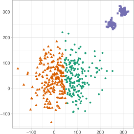
(a)

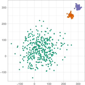
(b)

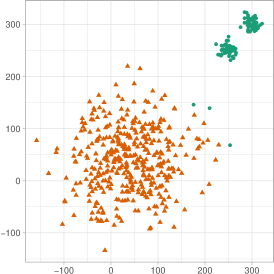
(c)

Figure 1: Clustering of the simulated dataset using (a) $k$-Means with $K=3$ and (b) Model Based Clustering with $K=3$ and (c) $k$-means clustering with $K=2$, which is also the optimal number of groups, as per the jump statistic.

Figure 1. The results clearly indicate that there is a distinction in the optimized solutions obtained using (well-initialized) $k$-means and GMMBC. In the first case (Figure LABEL:fig:1a), the $k$-means solution splits the larger cluster into two while combining the two smaller true clusters into one simply because of its predilection for homogeneous spherical groups. GMMBC has the ability to model mixing proportions and dispersions more generally, providing the correct solution here (Figure LABEL:fig:1b). To further illustrate pitfalls arising from potential model misspecification, we consider using well-initialized $k$-means solutions for $K=1,2,\ldots,10$. The jump statistic chooses $K=2$ as the optimal solution, which Figure LABEL:fig:1c shows more or less puts observations in the larger cluster into the first group and observations in the two smaller groups into the second. Three observations from the larger group that are closer to the combined center of the two (true) smaller groups are also misclassified. The choice of $K=2$ as the optimal grouping makes sense under the assumption of spherical homogeneous clusters governing $k$-means because the larger group is substantially well-separated from the two smaller ones which at some resolution can be grouped together as one cluster with a similar spherical dispersion structure as the larger one. This example illustrates the importance of the assumptions underlying the algorithms used in clustering and the challenges that may consequently arise in their interpretation.

2.3.3 Variable Selection in Clustering

An important issue in clustering is in deciding the variables that are relevant for the purpose. Several authors (e. g. Horváth, 2002; Horváth et al., 2008; Zitouni et al., 2015; Zhang et al., 2016) have used only $\log_{10}T_{90}$ while others (e.g. Veres et al., 2010; Horváth et al., 2004, 2006; Horváth et al., 2010) have used $\log_{10}T_{90}$ and $\log_{10}H_{32}$. Mukherjee et al. (1998) and Chattopadhyay et al. (2007) have used between three and six variables in their investigations. Redundancy in variables included for clustering can considerably degrade performance (see Raftery & Dean, 2006, who provided a variable selection approach for GMMBC). Specifically, Raftery & Dean (2006) formulated variable selection in terms of model selection, and proposed an effective way to remove irrelevant variables from a dataset. Their methodology partitions a set of variables ${\boldsymbol{\mathcal{X}}}$ into three subsets ${\boldsymbol{\mathcal{X}}}^{(1)}$, ${\boldsymbol{\mathcal{X}}}^{(2)}$ and ${\boldsymbol{\mathcal{X}}}^{(3)}$ where ${\boldsymbol{\mathcal{X}}}^{(1)}$ consists of the set of variables already selected for clustering, ${\boldsymbol{\mathcal{X}}}^{(2)}$ consists of the variable(s) under consideration for inclusion or exclusion from the set of clustering variables and ${\boldsymbol{\mathcal{X}}}^{(3)}$ denotes the other remaining variables. The decision to include or exclude ${\boldsymbol{\mathcal{X}}}^{(2)}$ from the set of clustering variables is taken based on the following two models on the entire dataset ${\boldsymbol{\mathcal{X}}}$:

$$\begin{split}\mathcal{M}_{1}:~{}P({\boldsymbol{\mathcal{X}}}|z_{1})&=~{}P({\boldsymbol{\mathcal{X}}}^{(1)},{\boldsymbol{\mathcal{X}}}^{(2)},{\boldsymbol{\mathcal{X}}}^{(3)}|z_{1})\\ &=~{}P({\boldsymbol{\mathcal{X}}}^{(3)}|{\boldsymbol{\mathcal{X}}}^{(2)},{\boldsymbol{\mathcal{X}}}^{(1)})P({\boldsymbol{\mathcal{X}}}^{(2)}|{\boldsymbol{\mathcal{X}}}^{(1)})P({\boldsymbol{\mathcal{X}}}^{(1)}|z_{1})\\ \mathcal{M}_{2}:~{}P({\boldsymbol{\mathcal{X}}}|z_{1})&=~{}P({\boldsymbol{\mathcal{X}}}^{(1)},{\boldsymbol{\mathcal{X}}}^{(2)},{\boldsymbol{\mathcal{X}}}^{(3)}|z_{1})\\ &=~{}P({\boldsymbol{\mathcal{X}}}^{(3)}|{\boldsymbol{\mathcal{X}}}^{(2)},{\boldsymbol{\mathcal{X}}}^{(1)})P({\boldsymbol{\mathcal{X}}}^{(2)},{\boldsymbol{\mathcal{X}}}^{(1)}|z_{1})\end{split}$$

where $z_{1}$ is the set of unobserved cluster memberships. Model $\mathcal{M}_{1}$ implies that ${\boldsymbol{\mathcal{X}}}^{(2)}$ gives no additional information about clustering while model $\mathcal{M}_{2}$ implies that ${\boldsymbol{\mathcal{X}}}^{(2)}$ provides additional information about clustering beyond that provided by the already-included ${\boldsymbol{\mathcal{X}}}^{(1)}$. $\mathcal{M}_{1}$ and $\mathcal{M}_{2}$ are compared using the Bayes Factor (8) with $B_{12}>1$ providing evidence that the set ${\boldsymbol{\mathcal{X}}}^{(2)}$ is redundant. As before, BIC provides a quick approximation. This results in the greedy search algorithm of Raftery & Dean (2006) which chooses or deselects variables as per improvement in BIC. At each stage the best combination of the number of groups and clustering model is chosen. A brief description of the forward- and backward-stepwise selection algorithm is as follows:

1. Select the first clustering variable as the one that provides the maximum evidence of univariate clustering.

2. The second clustering variable is selected such that it gives the highest evidence of bivariate clustering after including the first variable that was selected.

3. The next variable is proposed such that it shows the maximum evidence of clustering with the previously chosen variables included. The variable is accepted as a clustering variable if the evidence favours this outcome over not including it as a clustering variable.

4. The variable (from the current set of variables) for which the evidence of clustering including all the selected variables versus clustering including all the variables except the proposed variable is weakest is proposed to be removed from the current set of variables. This variable is removed if the evidence for clustering with its inclusion is weaker than the evidence to the contrary.

5. Steps 3 and 4 are iterated until two consecutive steps are rejected, at which point the procedure terminates.

This algorithm is implemented by the R package clustvarsel (Scrucca & Raftery, 2015) and we use it here.

2.4 Validity of Obtained Groupings

A difficult aspect of clustering, exacerbated for multivariate datasets, is cluster validation. Here, we discuss a few graphical and numerical ways for assessing our groupings.

2.4.1 The silhouette width

Rousseeuw (1987) developed the silhouette width as a popular but computationally intensive way for judging distance-based clustering results. The basic objective is to compare the similarity of an object to its own group members with that to observations in other groups. The silhouette value $\zeta_{i}$ for the $i$th observation lies in $[-1,1]$ with a high value indicating a close match of the observation with its own group and a poor match with others, thus satisfying the primary clustering goal of finding distinct homogeneous groups. The $\zeta_{i}$s are calculated for each observation with the distribution of these indices providing a measure of cluster validity. Operationally, $\zeta_{i}$ is calculated for the $i$th observation $\boldsymbol{x}_{i}$ assigned to $\mathcal{G}_{k}$ (say) via the following steps:

1. Calculate the average distance to all other observations in $\mathcal{G}_{k}$ (its own group). Call this average distance $\varpi_{i}$. Then, for $\boldsymbol{x}_{i}\in\mathcal{G}_{k}$, we have $\varpi_{i}=\sum_{j\in\mathcal{G}_{k}}d(\boldsymbol{x}_{i},\boldsymbol{x}_{j})/(n_{k}-1)$ where $n_{k}$ is the number of observations in $\mathcal{G}_{k}$.

2. Also, for each group $\mathcal{G}_{l},l\neq k$, obtain the average distance, $\vartheta^{(l)}_{i}$ of $\boldsymbol{x}_{i}$ to all $\boldsymbol{x}_{j}\in\mathcal{G}_{l}$. That is, calculate $\vartheta^{(l)}_{i}=\sum_{j\in\mathcal{G}_{l}}d(\boldsymbol{x}_{i},\boldsymbol{x}_{j})/n_{l}$. Let $\vartheta_{i}=\min_{l\neq k}\vartheta_{i}^{(l)}$ be the minimum of these average distances of $\boldsymbol{x}_{i}$ to the other groups.

3. The silhouette index for the $i$th observation is then

   $$\varsigma_{i}=\frac{\vartheta_{i}-\varpi_{i}}{\max(\varpi_{i},\vartheta_{i})}.$$

Clearly, $-1\leq\varsigma_{i}\leq 1$ $\forall$ $i$. In the above, $d(\boldsymbol{x}_{i},\boldsymbol{x}_{j})$ is the distance between $\boldsymbol{x}_{i}$ and $\boldsymbol{x}_{j}$, for which the Euclidean or any standard metric is used. However, while it is straightforward to use the Euclidean distance for calculating $\varsigma_{i}$s for $k$-means clusterings, the distance to be used with results from GMMBC and other clustering methods is not always clear.

2.4.2 Graphical Displays of Supervised Principal Components

Meaningful graphical displays are challenging propositions for datasets having more than two dimensions, so projections onto 2- or 3-dimensions have to be made in a way that the main features are presented. For grouped data, the main features to be presented are the between-groups separability and within-groups homogeneity. The goal then is to find the projection that best shows the separation of the groups in the data. The most popular statistical approach for dimensionality reduction is Principal Components Analysis (PCA) independently developed by Pearson (1901) and Hotelling (1933a, b) which projects (possibly) correlated variables into (a possibly lower number of) uncorrelated variables called Principal Components. PCA is an unsupervised learning tool sensitive to outliers, but more importantly in the context of grouped data, does not use this information and as such is not very useful in the context of finding projections that provide this sense of separation between groups. Weighted PCA (Koren & Carmel, 2004) is an alternative to PCA that can handle outliers depending on the choice of weights. The main objective is to find a $q$-dimensional projection ($q<p$, where $p$ is the dimensionality of $\boldsymbol{x}_{i}$s) that maximizes

$$\sum_{i<j}\upsilon_{ij}\delta^{2}_{ij}(q)$$ (9)

where $\delta^{2}_{ij}(q)$ denotes the Euclidean distance between two observations $\boldsymbol{x}_{i}$ and $\boldsymbol{x}_{j}$ in the $q$-dimensional projection space and ${(\upsilon_{ij})}^{n}_{i,j=1}$ denotes the symmetric pairwise non-negative weights (or dissimilarities). By convention, $\upsilon_{ii}\equiv 0$ $\forall$ $i$. Koren & Carmel (2004) propose to robustify PCA by choosing

$$\upsilon_{ij}=\frac{1}{\delta_{ij}}$$ (10)

where $\delta_{ij}\equiv\delta_{ij}(p)$ denotes the Euclidean distance between $x_{i}$ and $x_{j}$ in the original space. This choice of weights for weighted PCA yields Normalized PCA and can result in well-balanced projections (Koren & Carmel, 2004). It still remains to describe how the projection into the $q$-dimensional space should be carried out. Recall that the objective is to obtain the $q$-dimensional projection that maximizes (9). This is done by defining a $n\times n$ Laplacian matrix

$$L^{(\upsilon)}_{ij}=\begin{cases}\sum_{j=1}^{n}\upsilon_{ij}&i=j\\ -\upsilon_{ij}&i\neq j\end{cases}$$ (11)

and then obtaining the $q$-dimensional projections in terms of the eigenvectors corresponding to the $q$ largest eigenvalues of the matrix $\boldsymbol{X}^{T}\boldsymbol{L}^{(\upsilon)}\boldsymbol{X}$, where $\boldsymbol{X}^{T}=(\boldsymbol{x}_{1}\vdots\boldsymbol{x}_{2}\vdots\ldots\vdots\boldsymbol{x}_{n})$ is the $p\times n$ matrix containing the data.

Our description hitherto has not accounted for available label information in the data. This label information can be used to inform the weights and obtain the discriminating projection in $q$-space that will yield the projected distances $\delta_{ij}(q)$ that will separate out the groups, as far as possible, in the projected space. Koren & Carmel (2004) suggest tweaking the $\upsilon_{ij}$s for the $(\boldsymbol{x}_{i},\boldsymbol{x}_{j})$ pairs where both observations have the same class labels. Thus, they modify

$$\upsilon^{(\ell)}_{ij}(\tau)=\begin{cases}\tau\upsilon_{ij}&\text{if {i} and {j} have the same label}\\ \upsilon_{ij}&\text{otherwise}\end{cases}$$ (12)

where $0\leq\tau\leq 1$. A typical choice of $\tau$ is 0, though other values are possible. Proceeding with this specification of $\upsilon^{(\ell)}_{ij}$ leads us to modify $\boldsymbol{L}^{(\upsilon)}$ in Equation (11) to $\boldsymbol{L}^{(\upsilon^{(\ell)})}$ and to get the projections in the same manner as for normalized PCA. Projections of the data thus obtained provide us with supervised principal components and the methodology is called Supervised PCA (SPCA). Note that calculation of $\delta_{ij}$s in the original space has been proposed using Euclidean distance. This distance is again natural to use $k$-means-clustering results, but the distance to be used for results from GMMBC is not always clear.

2.4.3 Measuring distinctiveness of groups via the overlap

An overlap measure typically indicates the extent to which clusters obtained through a method are distinct from another and thus can be used to judge the goodness of the clustering. In the context of GMMs, Maitra & Melnykov (2010) defined overlap between two Gaussian clusters as the sum of their misclassification probabilities. For the general GMM, these measures are somewhat involved (see Theorem 1 of Maitra & Melnykov, 2010) but for the special case of the $k$-means solutions the pairwise overlap between the $k$th and the $l$th cluster can be defined as $\omega_{kl}==2\Phi(-\|\boldsymbol{\mu}_{k}-\boldsymbol{\mu}_{l}\|/2\sigma)$ where $\Phi(\cdot)$ is the $p$-variate Gaussian density, $\boldsymbol{\mu}_{k}$ and $\boldsymbol{\mu}_{l}$ are the $k$th and the $l$th cluster means and $\sigma$ is the common (homogeneous) standard deviation for each group, estimated unbiasedly as $W_{K}/((n-K)p)$ with $W_{K}$ as the optimized value of (1). In either case, for a dataset partitioned into $K$ groups, we can obtain a $K\times K$ matrix $\Omega$ of pairwise overlap measures. Summarizing this matrix is not easy, so Melnykov & Maitra (2011) (see manual) developed the generalized overlap $\ddot{\omega}$ by borrowing a summary measure from Maitra (2010). Specifically, they proposed $\ddot{\omega}=(\lambda_{(1)}-1)/{(K-1)}$, where $\lambda_{(1)}$ is the largest eigenvalue of $\Omega$. Smaller values of $\ddot{\omega}$ are expected to indicate the most distinctive groupings. The R package MixSim (Melnykov et al., 2012) calculates the pairwise and generalized overlap measures through the overlap() and overlapGOM() functions, respectively. Referring back to the example in Figure 1 we calculate $\ddot{\omega}$ to be 0.126 for the clustering of Figure LABEL:fig:1a, $2.932\times 10^{-5}$ for the grouping of Figure LABEL:fig:1b and 0.005 for the partitioning in Figure LABEL:fig:1c, respectively. Despite the good agreement here with the correct clustering solution, we note that $\ddot{\omega}$ is only a worthwhile diagnostic in the assessment of the obtained clustering and not necessarily a mechanism to determine the best clustering solution for which BIC here provides the correct answer.

3 Cluster Analysis of GRBs

The BATSE catalog provides temporal and spectral information for many GRBs. Of interest to us are the parameters:

$T_{50}$:

The time by which 50% of the flux arrive.

$T_{90}$:

The time by which 90% of the flux arrive.

$P_{64}$, $P_{256}$, $P_{1024}$:

The peak fluxes measured in bins of 64, 256 and 1024 milliseconds, respectively.

$F_{1}$, $F_{2}$, $F_{3}$, $F_{4}$:

The four time-integrated fluences in the 20-50, 50-100, 100-300, and $>$ 300 keV spectral channels, respectively.

Mukherjee et al. (1998) identified three more composite variables used by researchers for studying GRBs. These are:

$F_{t}$=$F_{1}+F_{2}+F_{3}+F_{4}$:

The total fluence of a GRB.

$H_{32}=F_{3}/F_{2}$:

Measure of spectral hardness using the ratio of $F_{2}$ and $F_{3}$.

$H_{321}=F_{3}/(F_{1}+F_{2})$:

Measure of spectral hardness based on the ratio of channel fluences $F_{1},F_{2},F_{3}$.

The current BATSE catalog, that is, the BATSE 4Br catalog (Paciesas et al., 1999) contains bursts from the BATSE 3B catalog studied by Mukherjee et al. (1998) along with 515 additional bursts between 20 September 1994 and 29 August 1996. The BATSE 4Br catalog also contains revised locations for 208 bursts from the BATSE 4B catalog analyzed by Chattopadhyay et al. (2007). The BATSE 4Br Catalog (and also the BATSE 4B and older catalogs) has several zero entries for the four integrated time fluences $F_{1}$, $F_{2}$, $F_{3}$, $F_{4}$. There is also one zero entry for the peak fluxes.

Table 1: Number ($n_{j}$) of observations with zeroes in each of the BATSE 4Br catalog parameters (denoted by $X_{j}$).

$X_{j}$	$T_{50}$	$T_{90}$	$P_{64}$	$P_{256}$	$P_{1024}$	$F_{1}$	$F_{2}$	$F_{3}$	$F_{4}$
$n_{j}$	0	0	1	1	1	29	12	6	339

Table 1 provides the number of zero observations for each field in the BATSE 4Br catalog. How these zero entries should be included in the analysis can determine the quality of our results, especially if these zeroes are indicators for anomalous or missing values rather than numerical values. This has particular impact in the context of variables derived using $F_{4}$, for which there are as many as 339 zero values. Mukherjee et al. (1998) and Chattopadhyay et al. (2007) have performed their analyses on the BATSE 3B and 4B catalogs, respectively, after dropping these zero entries. Horváth et al. (2006) analyzed the BATSE 4Br catalog, but they restricted their attention only to $\log_{10}T_{90}$ and $\log_{10}H_{32}$ for which 1956 GRBs have non-zero observations in both the $F_{2}$ and $F_{3}$ parameters that go into calculating $H_{32}$.

It would be instructive to find out how the zeroes in the parameters occur. To obtain more information in this regard, we contacted the BATSE GRB team with our questions. A team member, Charles A. Meegan has, in personal communication, explained that “the zero values ultimately derive from the fact that a model background, determined from data before and after the burst, must be subtracted from the signal during the burst. Occasionally, fluctuations in the background lead to a negative value for the burst fluence. This is most prevalent in the lowest and highest channels of the weaker bursts, where the intensity is generally low.. Since a negative fluence is unphysical, these values were set to zero in the catalog.” He went on to add that in these cases, the quoted error bar is to be interpreted as a $1-\sigma$ upper limit. Further details on how the background calculations and subtractions are done is provided in Pendleton et al. (1994)’s analysis of the first BATSE catalog. Thus, the recorded zeroes in the BATSE catalog for these parameters are not numerical values, but rather records of uncertain values. Table 1 provides further support of this assertion because most zeros are in the fluences $F_{1}$ and $F_{4}$. Therefore, the only appropriate approach to treat these GRBs with zero parameters as essentially having missing observations in those parameters. (We have also verified that the 1594 GRBs used in Chattopadhyay et al. (2007) are among the 1599 BATSE 4Br GRBs without any zero parameters – the balance five GRBs have trigger numbers 107, 2450, 6368, 6404 and 6645.) Therefore, in the absence of clustering methods for partially observed data, we exclude GRBs missing any parameter from our cluster analysis.

The missing observations in the four integrated time fluences mean that computation of the composite variables $F_{t}$, $H_{32}$ and $H_{321}$ is not possible for all the 1973 GRBs in the BATSE 4Br catalog. (The one case with zeroes for the peak flux parameters also has zero readings for the integrated time fluences and is therefore part of the GRBs missing $F_{1}$, $F_{2}$, $F_{3}$ or $F_{4}$.) . Thus after excluding the incomplete GRBs the 4Br catalog has 1599 GRBs containing complete information on the six variables $T_{50}$, $T_{90}$, $P_{256}$, $F_{t}$, $H_{32}$ and $H_{321}$.

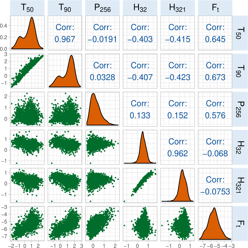
Figure 2: A matrix of scatterplots (the lower triangular portion), density plots ( the diagonal) and correlation coefficients(the upper triangular portion) of the base-10 logarithms of the six parameters $T_{50}$, $T_{90}$, $P_{256}$, $H_{32}$, $H_{321}$, $F_{t}$ using 1599 GRBs of the BATSE 4Br catalog.

Mukherjee et al. (1998) used these six variables, namely $\log_{10}T_{50}$, $\log_{10}T_{90}$, $\log_{10}P_{256}$, $\log_{10}F_{t}$, $\log_{10}H_{32}$ and $\log_{10}H_{321}$ for hierarchical clustering and three ($\log_{10}T_{90}$, $\log_{10}F_{t}$ and $\log_{10}H_{321}$) variables for GMM-based analysis on 797 GRBs (having observations on all these parameters) from the BATSE 3B catalog. Chattopadhyay et al. (2007) used all six of these variables in their cluster analysis of the GRBs from the BATSE 4B catalog. We also revisit cluster analysis of the GRBs using the BATSE 4Br catalog using these six variables. Analysis of these six variables means that we can only consider for analysis the 1599 GRBs for which readings on all the parameters are available. However, this leaves out 374 GRBs. Of these, only 44 GRBs have $F_{t}$ missing. Thus, there are 1929 GRBs with information on five parameters $T_{50}$, $T_{90}$, $P_{256}$, $H_{32}$ and $H_{321}$. We analyze these GRBs separately also in order to get an indication on whether the clustering properties of this larger set of GRBs are similar to that of the 1599 GRBs with data on all six parameters.

We first briefly discuss the univariate and bivariate relationships between the six parameters in the BATSE 4Br catalog. Figure 2 displays the bivariate scatterplots along with the correlation coefficients and univariate density plots of the six parameters. The two duration variables $\log_{10}T_{50}$ and $\log_{10}T_{90}$ and the two hardness ratios $\log_{10}H_{32}$ and $\log_{10}H_{321}$ show very high positive association between themselves. High positive associations are also seen between the duration variables and the total fluence $\log_{10}F_{t}$. The peak flux $\log_{10}P_{256}$ and $\log_{10}T_{90}$ exhibits a weak positive association among themselves. The association of $\log_{10}P_{256}$ with $\log_{10}T_{50}$ is weakly negative while the association between either duration variable and each hardness ratios is also moderate. Note also that the logarithmic transformations on each of the parameters has reduced skewness appreciably, as seen in the univariate density plots displayed along the diagonal of Figure 2.

Beyond the associations, the scatterplots of Figure 2 show the limitations posed by bivariate and univariate summaries, as was also discussed by Mukherjee et al. (1998). Both $\log_{10}T_{50}$ and $\log_{10}T_{90}$ are bimodal in their univariate densities, but none of the bivariate figures show much grouping. Thus, any grouping in the GRBs, if they exist, are in dimensions higher than two and can not be recovered by considering only univariate or bivariate summaries. A reviewer has pointed out that Bagoly et al. (1998) have used the first two principal components to perform clustering in a bivariate framework: note, however, that Chang (1983) has demonstrated theoretically as well as by simulations and in applications to real data, that the principal components with the largest eigenvalues do not necessarily contain the most information about the cluster structure, and that taking a subset of principal components can lead to a major loss of information about the groups in the data. Similar concerns have also been expressed by other authors (see, e.g. Green & Krieger, 1995; Yeung & Ruzzo, 2001; Kettenring, 2006). We now perform cluster analysis on the 1599 GRBs with observations using all six parameters $\log_{10}T_{50}$, $\log_{10}T_{90}$, $\log_{10}P_{256}$, $\log_{10}F_{t}$, $\log_{10}H_{32}$ and $\log_{10}H_{321}$.

3.1 Clustering GRBs Using all Six Parameters

We first perform $k$-means clustering of the 1599 GRBs in the BATSE 4Br and then move on to GMMBC.

3.1.1 $k$-means clustering

We revisited Chattopadhyay et al. (2007)’s analysis (done on 1594 complete observations of the BATSE 4B catalog) by performing $k$-means clustering with $K=1,2,\ldots,20$ groups on the 1599 BATSE 4Br observations. Similar to the approach of Mukherjee et al. (1998), Chattopadhyay et al. (2007) and other authors, and from the density plots of Figure 2, we analyzed all parameters in the logarithmic scale. Further, because these parameters measure different quantities, they were also individually scaled to have the same standard deviation. To allay the effects of initialization, for each $K$ we initialized our $k$-means algorithms using both deterministic and stochastic methods. We first initialized $k$-means with the results obtained upon performing hierarchical clustering using the Ward (1963) criterion and then cutting the resulting tree at $K$ groups. The algorithm was then run to convergence from these hierarchically-obtained means. An alternative approach ran $k$-means to convergence from each of $10Knp$ random starts, as per MacQueen (1967) with each start simply being $K$ (unique) randomly-chosen GRBs. The best of all these converged $k$-means solutions – where best means the solution providing the smallest value of $W_{K}$ as per Equation (1) - is taken to be the $k$-means solution for that $K$. The objective behind so many initializations is to reduce the chance that our $k$-means solutions for any $K$ have not arrived at a global optimum. We also followed Chattopadhyay et al. (2007) in using the Jump statistic (Sugar & James, 2003) to decide on the optimal number of groups.

Figures 3a and 3b respectively display the distortion and the jump curves of the $k$-means solutions for $K=1,2,\ldots.20$. There is not much leveling off of the kind found in Chattopadhyay et al. (2007) for either the distortion curve or the jump statistic. Indeed, the distortion curve keeps on trending down with decreasing $K$, while the jump statistic generally trends up with increasing $K$. Our results are somewhat contrary to those of Chattopadhyay et al. (2007). Looking back at their results, it appears from Figure 1 of their paper that $K=4$ had the highest value of the jump statistic, and the distortion curve did not level off even in that paper. We also see the near-imperceptible dip in the jump curve

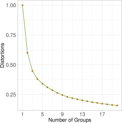
(a)

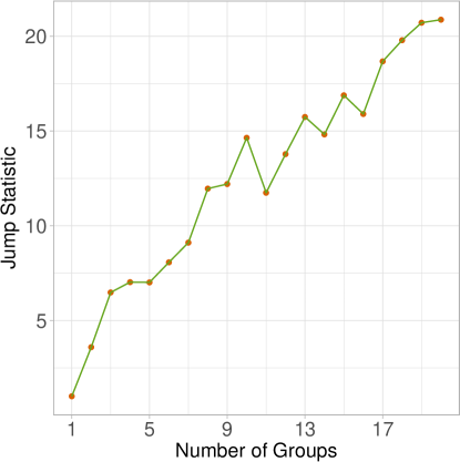
(b)

Figure 3: (a) The distortion and (b) jump curves for $k$-means clustering solutions of the GRBs.

for $K=5$ but that is very quickly reversed for $K=6$ and beyond. We also tried the methods of Maitra et al. (2012) to assess the question as to whether a larger $K^{\prime}$-means clustering solution fits the data significantly better than a smaller $K$-means one ($K^{\prime}>K$) and were able to reject the null hypothesis of no significant improvement on fitting the larger model over the smaller model for all $(K,K^{\prime})$-pairs, with $1\leq K<K^{\prime}\leq 20$. All the tests reported negligible $p$-values which means that significantly better fits are provided by larger $K$. This points to the possibility that actual groups in the GRBs may have general-shaped and unequal dispersions (spreads). Stipulating a homogeneous spherical structure on them in this situation (as $k$-means inherently does) leads to significantly better fits with solutions that model each general dispersion structure with sets of homogeneous spherical dispersions, each centered in different regions of the ellipsoidal-structured groups.

(a)

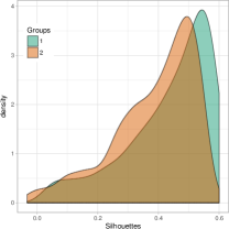
(b)

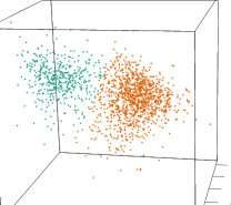
(c)

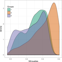
(d)

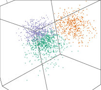
(e)

Figure 4: (a) Distributions of the silhouette widths obtained for the $k$-means clustering of the GRB, for $2,3,\ldots,13$ groups. (b) Group densities of the silhouette widths and (c) three-dimensional projection plot of the SPCAs for the 2-means solutions. (d) Group densities of the silhouette widths and (e) three-dimensional projection plot of the SPCAs for the 3-means solutions.

We also evaluated cluster validity via the silhouette widths for each observation and at each $K$. We display in Figure 4a the individual silhouette widths through a kernel density plot (violin plot). Like a boxplot, a violin plot (Hintze & Nelson, 1998) represents distributions of data through medians and the quartiles and extrema, but additionally displays the density of the data (here, the silhouette widths ) at different values. For clarity, we only display the silhouette indices for $K=2,3,\ldots,13$ but the values are fairly similar for higher $K$. There appears to be greater validity for $K=2$ than for other $K$, but there is considerable overlap between the distributions of the silhouette indices for $K=2$ and the ones for the other $K$.

We now further investigate the groups formed by the 2- and 3-means solutions. Figure 4b displays the densities of the silhouette widths of the GRBs assigned to each of the groups in the 2-means solution. The distribution shows that most of the silhouette widths for both groups have moderate to moderately high values and so have high cluster validity. However, there is a sizable minority of GRBs that do not have high silhouette widths, and some even have negative values. This finding is supported by Figure 4c which is a three-dimensional display of the three best SPCA projections. The display in Figure 4c presents what in our view is the perspective showing the best separation between the groups (see the supplementary materials for HTML code providing the interested reader the ability to try out other perspectives). The two groups are similarly-shaped and sized with somewhat distinct cores, but there are also many observations from one group that could easily have arisen from the other. Indeed, it would be quite difficult in the figure to demarcate the two groups in the absence of color. Figure 4d and Figure 4e show corresponding distributions of the group silhouette widths and the three-dimensional SPCA projections (HTML code in the supplement) for the 3-means clustering of the GRBs. Once again, there are small values for many of the silhouette widths, indicating some discomfort with the clustering. Note also that the most separated group as per Figure 4e has substantially moderately high silhouette widths, while the other two groups are similar, mostly having moderate values. This illustration indicates the pitfalls with using $k$-means clustering on the GRBs. As the number of groups increases, $k$-means prefers breaking up the observations into smaller and smaller equi-sized spherically dispersed groups, but as viewed by the small silhouette widths in the Figure 4a, even this is not completely adequate. Numerically, the generalized overlap for $K=2$ is 0.028 while that for $K=3$ is 0.044. Therefore, our investigations indicate not much support for Chattopadhyay et al. (2007)’s finding of a preferred $3$-means solution for grouping GRBs. Indeed, given our results, we do not find much appeal for $k$-means-type clustering solutions for understanding the heterogeneities in GRBs. We therefore proceed with GMMBC for further analysis of GRBs.

3.1.2 Gaussian Mixture Models-based Clustering

Mukherjee et al. (1998) performed GMMBC on the BATSE 3B catalog data using three of the six variables (log$T_{50}$, log$T_{90}$, log$P_{256}$, log$F_{t}$, log$H_{32}$ and log$H_{321}$). Using visual inspection (See Figure 1 of Mukherjee et al., 1998), the authors identified highly redundant variables and performed GMMBC using only $T_{90}$, $F_{t}$ and $H_{321}$. Other authors (Horváth, 2002; Horváth et al., 2008; Zitouni et al., 2015; Zhang et al., 2016) have used only $\log_{10}T_{90}$ while others (e.g. Veres et al., 2010; Horváth et al., 2004, 2006; Horváth et al., 2010) have used $\log_{10}T_{90}$ and $\log_{10}H_{32}$ in their respective cluster analyses. Chattopadhyay et al. (2007) used all six variables in their GMMBC. Recent advances in this field motivated us to reexamine the issue of redundancy among these six variables in the context of clustering and using the formal GMMBC-based variable selection methods discussed in Section 2.3.3. We used clustvarsel (Scrucca & Raftery, 2015) to perform GMMBC variable selection using $\log_{10}T_{50}$, $\log_{10}T_{90}$, $\log_{10}P_{256}$, $\log_{10}F_{t}$, $\log_{10}H_{32}$ and $\log_{10}H_{321}$. The results of the forward- and-backward-selection variable selection algorithm are presented in Table 2

Table 2: Results of the forward- and backward-variable selection step for determining redundancy of $\log_{10}T_{90}$, $\log_{10}T_{50}$, $\log_{10}H_{321}$, $\log_{10}H_{32}$, $\log_{10}P_{256}$, $\log_{10}F_{t}$ in GMMBC.

Step	Variable	Step Type	BIC Difference	Decision
1	$\log_{10}T_{90}$	Add	452.95	Accepted
2	$\log_{10}T_{50}$	Add	395.74	Accepted
3	$\log_{10}H_{321}$	Add	176.59	Accepted
4	$\log_{10}H_{321}$	Remove	176.95	Rejected
5	$\log_{10}H_{32}$	Add	443.06	Accepted
6	$\log_{10}T_{50}$	Remove	273.56	Rejected
7	$\log_{10}P_{256}$	Add	260.28	Accepted
8	$\log_{10}T_{50}$	Remove	235.61	Rejected
9	$\log_{10}F_{t}$	Add	185.52	Accepted
10	$\log_{10}T_{50}$	Remove	194.60	Rejected

and indicate scant support for the theory of redundancy among the six variables for clustering: we therefore proceed, using all of them (in the logarithmic scale) in our GMMBC.

Chattopadhyay et al. (2007) performed GMMBC but with a Dirichlet Process prior to decide on the number of components. However, there is not much software matching the modeling flexibility of mclust (Fraley et al., 2012) or the enhanced initialization and fast computational approaches of EMCluster (Chen & Maitra, 2015a, b). We therefore use these packages for GMMBC of the GRBs for each $K=1,2,\ldots,9$ and chose for each $K$ the solution with the highest loglikelihood. The BIC was also calculated for each $K$: these are displayed in Figure 5.

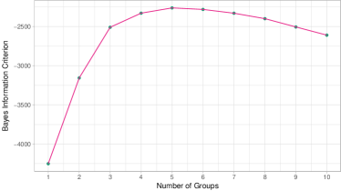
Figure 5: Plot of BIC with $K$ upon performing GMMBC of the 1599 GRBs in the BATSE 4Br catalog.

From that figure, it is clear that amongst all GMMs, a mixture of five Gaussian densities provides the best fit to the GRB dataset. Thus, there is evidence of five kinds of GRBs in the BATSE catalog. This finding is at variance with studies published in the literature which have identified at most three distinct groups. Chattopadhyay et al. (2007) used all six variables and the BATSE 4B GRBs and found three groups, but most of the other classifications used only the duration variables. (We note that our results here used the BATSE 4Br catalog, but we also separately performed the analysis on the older BATSE 4B dataset with 1594 complete observations and obtained a similar five-groups solution. This provides greater confidence in our findings.)

Validity of the GMMBC Solution:

The distance-based silhouette widths or the SPCA displays can not be calculated for results obtained using GMMBC with general dispersion matrices. So we only discuss the overlap measures between the different groups and the generalized overlap measures for $K$-components-fitted GMMBC solutions ($K=2,3,4,5$) as reported in

$K$	$\ddot{\omega}$
2	0.17
3	0.12
4	0.11
5	0.10

(a)

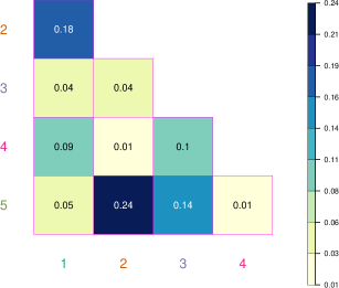
(b)

Figure 6: (a) Generalized overlap ($\ddot{\omega}$) measures for the 2-, 3-, 4- and 5-components GMMBC solutions of the 1599 BATSE 4Br GRBs. (b) Pairwise overlap measures between the $k$ and the $l$th groups in the 5-component GMMBC solution as indicated by the margins. Color in the margins correspond to the group indicator that is the same for all displays and tabulations involving the five-component GMMBC fits to the dataset with six parameters.

the table in Figure 6a where the $K=5$ model marginally presents the most separated components over $K=4$, with both solutions providing more distinct components than the GMMs with $K=2$ or 3 components. We note that the generalized (and also our pairwise) overlap measures are based on the population mixture model components with parameters estimated from the data. Thus, the values are calculated under the assumption of the GMM that provides the best fit to the data.

The BIC and the generalized overlap measures provide additional indication on the presence of five distinct kinds of GRBs. We now comprehensively evaluate the five classes of GRBs that we have obtained from our analysis.

Analysis of Results

Figure 6b displays the pair-wise overlap measures between the five groups in the five-component GMMBC fit to the data. The pairwise overlap measures indicate that the fourth group is the most distinct from all the others while the fifth group has substantial overlap with the second and third groups. The second and third groups are fairly distinct from each other however, so one may consider describing these groups themselves as a mixture of three-components (Baudry et al., 2010), but descriptions and characterizations of such merged groups are harder and less interpretable. Figure 6b also indicates distinctiveness between the first and the third groups, and (to a lesser extent) between the first and the fifth groups.

Table 3a tabulates the number of observations in each of the five groups. (The color for each group indicator in the table corresponds to the identities for each group and, for easy reference, hold for all displays and tabulations that refer to the 5-component GMMBC clusterings.) Clearly, the second and fifth groups have the most GRBs while the third group has the fewest GRBs. Table 3b provides the five group means from the GMMBC of GRBs. We also display parallel coordinate plots of all the observations with lines colored as per their classifications (Figure 7). A parallel coordinate plot (Inselberg, 1985; Wegman, 1990) is an effective way to visualize data containing multiple dimensions, where lines link the observation value for each coordinate. The coordinates themselves are displayed vertically on the same scale and are equi-spaced. These coordinate axes are called the parallel axes and a point in the $p$-dimensional space is represented as a polyline with vertices on these parallel axes. The position of the ith axis corresponds to the ith coordinate of the point (see Inselberg, 1985; Wegman, 1990). We use the parallel coordinates plot in Figure 7 to visually inspect the five groups and draw conclusions.

Table 3: (a) Number of GRBs and (b) Means of the six parameter values in each of the five groups identified by GMMBC.

Group	1	2	3	4	5
Number of observations	174	551	149	292	433

(a) Number of observations in each group

$k$	$\log T_{50}$	$\log T_{90}$	$\log P_{256}$	$\log H_{32}$	$\log H_{321}$	$\log F_{t}$
1	0.337	0.703	-0.150	0.536	0.232	-6.074
2	1.142	1.519	0.058	0.372	0.101	-5.405
3	-0.234	0.547	0.697	0.545	0.314	-5.594
4	-0.657	-0.312	0.240	0.795	0.617	-6.159
5	1.032	1.557	0.519	0.511	0.274	-4.838

(b) Mean parameter values for each group

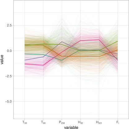
Figure 7: Parallel coordinate plot of the 1599 BATSE 4Br GRBs colored as per their group indicators. The solid lines represent the group medians for each of the six variables displayed. Variables are in the logarithmic scale.

(a) Group 1

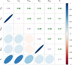
(b) Group 2

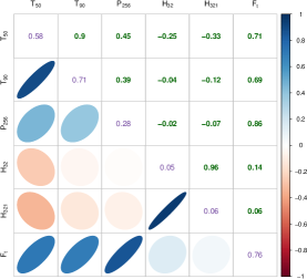
(c) Group 3

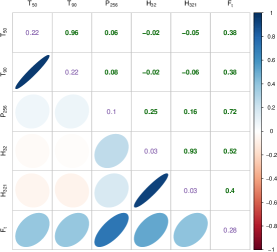
(d) Group 4

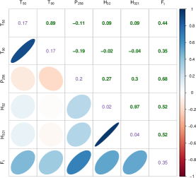
(e) Group 5

Figure 8: Variances and displays of the estimated correlations for each of the five groups obtained from the 5-component GMMBC solution of the 1599 GRBs. For each group, the off-diagonal elements display correlation between the variables while the diagonals display the variances. Both correlations and variances are calculated for the variables in the base-10 logarithmic scale.

To assess the properties of the five groups optimally found by GMMBC and BIC, we study the duration variable $\log_{10}T_{90}$ and the fluence variable $\log_{10}F_{t}$. These two variables were used by Chattopadhyay et al. (2007) and Mukherjee et al. (1998) to understand properties of groups obtained by them. We also consider interpretation of our results using these two variables to facilitate easy comparison with the findings of Chattopadhyay et al. (2007) and Mukherjee et al. (1998). Our fourth group (which is also the most distinct as per the pairwise overlap) consists of bursts of the shortest duration (about 0.5s) while burst durations of the first and third groups are around 5s and 3s, respectively. The fluences are also the highest for the second and fifth groups, both also having the longest durations of bursts. The fourth group (with shortest-duration bursts) has the lowest fluence. As mentioned in Section 1, the popular classification scheme classifies GRBs as short bursts ($T_{90}<2s$) and long bursts ($T_{90}>2s$). Following this framework, bursts of the fourth group can be designated as short duration bursts. Chattopadhyay et al. (2007) further classified bursts with $T_{90}>2s$ into two groups, the long-duration low-fluence bursts and the long-duration high-fluence bursts. Following their rationale, our first and third groups can be designated as having long-duration bursts with low fluence while our second and fifth groups can be categorized as those with long duration bursts with fluence higher than that of the first and third groups. It is also of interest to compare the GMMBC results of Mukherjee et al. (1998) on the smaller complete BATSE 3B GRBs with our groupings. Indeed, the three groups obtained by Mukherjee et al. (1998) have a good amount of similarity (in terms of the group means) with three of our groups. For example, the group mean of $\log_{10}T_{90}$ obtained by Mukherjee et al. (1998) for their three groups were around $1.55$, $-0.42$ and $0.71$ which are quite similar to the means of our first, fourth and fifth groups. Actually, our second and fifth groups are quite similar for $\log_{10}T_{90}$ to the mean of the first group of Mukherjee et al. (1998). Our first group also shows considerable similarity to the third group (again in terms of $\log_{10}T_{90}$ ) obtained by Mukherjee et al. (1998). The other variables also exhibit similar resemblance with the results of Mukherjee et al. (1998).

Mukherjee et al. (1998) described group properties using the hardness ratios in addition to duration and total fluence. Thus, they classified their three groups using the three properties Duration/Fluence/Spectrum. Using this rule the three groups obtained by them were summarized as long/bright/intermediate, short/faint/hard and intermediate/intermediate/soft. Adopting this rule, we find that our five groups can be classified in terms of intermediate/faint/intermediate, long/intermediate/soft, intermediate/intermediate/intermediate, short/faint/hard and long/bright/intermediate.

In addition to studying the means for understanding group properties, we also calculated the correlations between the six variables in each of the five classes. Figure 8 displays the correlation structures for the five GMMBC groups. The diagonals of each display provide the estimated group variances of the six variables obtained by GMMBC. The $(i,j)$th cell in the upper off-diagonal part of the display provides the numerical value of the correlation coefficient between the $i$th and $j$th variables while the lower off-diagonal $(j,i)$th cell provides a diagrammatic representation of the same correlation coefficients. The extent of linear relationship between any two variables in each of the clusters can then be easily represented using these visual representations. The relationships between the six variables for each of the five groups can also be understood by looking at correlation displays of Figure 8. For each of the five groups, the two duration variables $\log_{10}T_{50}$ and $\log_{10}T_{90}$ are very strongly correlated as are the hardness ratios $\log_{10}H_{32}$ and $\log_{10}H_{321}$. On the other hand, $\log_{10}T_{90}$ and $\log_{10}H_{321}$ exhibit moderately negative association in the first and third groups while they are weakly (negatively) correlated in the fourth and the fifth groups and moderately positively correlated in the second group. The duration $\log_{10}T_{90}$ and fluence $\log_{10}F_{t}$ exhibit moderate positive association in the fourth and fifth groups and strong positive association in the other three groups. There is weak negative association between $\log_{10}P_{256}$ and $\log_{10}F_{t}$ in the first group, a moderately positive association in the second group and strong positive correlation between these two parameters in the other groups. In summary, our identified groups have similar properties in the common variables as the groups in Mukherjee et al. (1998), but we also identify additional structure by including the additional variables ignored by them but declared relevant by variable selection.

3.2 Clustering the 1929 GRBs using complete information on five parameters

We now perform GMMBC using the five variables on the 1929 GRBs for which complete observations on $\log_{10}T_{50}$, $\log_{10}T_{90}$, $\log_{10}P_{256}$, $\log_{10}H_{32}$ and $\log_{10}H_{321}$ are available. Our objective here is to assesswhether the groups found by clustering the 1599 GRBs with six parameters adequately explain the kinds of GRBs generally available in the BATSE 4Br catalog. After obtaining the GMMBC for the optimal $K$ as per BIC, we identify the groups and study their properties in relation to the groups identified in Section 3.1.2. Our investigative framework mirrors Section 3.1.2 so we report results in brief.

3.2.1 Results

We again first scout for redundancy among these five variables for clustering the 1929 GRBs using the variable selection algorithm of Section 2.3.3 with the clustvarsel package in R. Table 4 indicates that all five variables contain relevant clustering information, and none of them are redundant, a result that is not wholly surprising in the light of the results of Table 2. Proceeding as before with GMMBC using the five variables $\log_{10}T_{50}$, $\log_{10}T_{90}$, $\log_{10}P_{256}$, $\log_{10}H_{32}$ and $\log_{10}H_{321}$, we find that the BIC is again optimal for $K=5$, as per Figure 9. The generalized overlap measures for $K=2,3,4,5$ are reported in the table of Figure 10a and show negligible differences between $K=3,4,5$ for each of which $\ddot{\omega}$ is around 0.11. Thus, though BIC clearly indicates that $K=5$ is the clear winner, there is not much difference in terms of separation of the clusters between either of the $K=3,4,5$ solutions. (We remind the reader of our comment at the end of Section 2.4.3 that $\ddot{\omega}$ is a diagnostic for evaluating the distinctiveness and quality of the obtained clustering while BIC is a metric for choosing $K$.) Note also that the separation is far higher for $K=5$ than for $K=3$ in the table of Figure 6a, which indicates that the additional relevant clustering information provided by $\log_{10}F_{t}$ (which can not be used here because of missing observations) provides more distinct groups.

Table 4: Results of stepwise variable selection algorithm for determining redundancy of $\log_{10}T_{90}$, $\log_{10}T_{50}$, $\log_{10}P_{256}$, $\log_{10}H_{321}$, $\log_{10}H_{32}$, for GMMBC of the 1929 five-parameter GRBs.

Step	Variable	Step Type	BIC Difference	Decision
1	$\log_{10}T_{90}$	Add	533.01	Accepted
2	$\log_{10}T_{50}$	Add	478.64	Accepted
3	$\log_{10}P_{256}$	Add	247.12	Accepted
4	$\log_{10}P_{256}$	Remove	247.52	Rejected
5	$\log_{10}H_{321}$	Add	252.34	Accepted
6	$\log_{10}H_{321}$	Remove	245.97	Rejected
7	$\log_{10}H_{32}$	Add	711.53	Accepted
8	$\log_{10}T_{50}$	Remove	271.56	Rejected

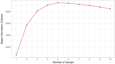
Figure 9: Plot of BIC against $K$ for GMMBC with 5 parameters.

$K$	$\ddot{\omega}$
2	0.14
3	0.11
4	0.11
5	0.11

(a)

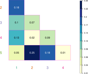
(b)

Figure 10: (a) Generalized overlap ($\ddot{\omega}$) measures for the 2-, 3-, 4- and 5-component GMMBC solutions of the 1929 BATSE 4Br five-parameter GRBs. (b) Pairwise overlap measures between the $k$ and the $l$th groups of the 5-groups solution as indicated by the margins. Here margin color corresponds to the group indicator that is the same for all displays and tabulations involving the five-component GMMBC fits to the five-parameter dataset.

Analysis:

Figure 10b displays the pairwise overlaps between the five groups in the five-component GMM fit to the 1929 GRBs. As in Figure 6b, the fourth group is the most distinct. Also, the fifth group shows a substantial amount of overlap with the second and third groups. Note that most of the pairwise overlap measures for the five groups in the six-parameter analysis (Figure 6b) are considerably lower than the pairwise overlaps for the five groups in the current five-parameter analysis indicating that the groups are now less distinct upon exclusion of $\log_{10}F_{t}$, which as per Table 2 contains relevant clustering information.

GMMBC of the 1599 GRBs using complete observations on six parameters ($\log_{10}T_{50}$, $\log_{10}T_{90}$, $\log_{10}P_{256}$, $\log_{10}H_{32}$, $\log_{10}H_{321}$ and $\log_{10}F_{t}$) and the 1929 GRBs using complete observations on the five parameters (with $\log_{10}F_{t}$ excluded from the above list) both yielded five groups as per BIC. It would be of interest to compare the two groupings. Table 5 tabulates the groups assigned to the 1929 GRBs under each of the two classifications. Indeed, 330 of these GRBs could not be classified under the GMMBC of Section 3.1.2 because of missing $F_{t}$s (and are assigned NA under the grouping of Section 3.1.2). It is interesting to note that a clear majority of the 330 GRBs that could not be clustered in Section 3.1.2 appear to be of the second kind, with the other kinds being fairly evenly represented but for the third group which only has 18 GRBs. The high values in the diagonal elements indicate that the overall grouping structure agrees quite well under both analyses. It is however, interesting to note that the second and the fifth groups have the most mismatches for both cases. (These are also the two largest classes in both groupings.) A plausible reason for these mismatches may be the loss of relevant clustering information by our having to exclude $F_{t}$ in order to perform GMMBC of the 1929 GRBs.

Table 5: Number of 1929 GRBs assigned to each grouping using GMMBC of 1599 GRBs using complete information on all six parameters (Grouping I) and GMMBC of 1929 GRBs using complete information on five parameters (Grouping II). GRBs which are missing the sixth parameter ($F_{t}$) can not be assigned under Grouping I and are placed in the NA category.

		Grouping I (from GMMBC of 1599 GRBs)
		1	2	3	4	5	NA	Total
Grouping II	1	78	3	7	1	0	40	129
	2	71	456	1	3	36	200	767
	3	1	11	130	3	17	18	180
	4	18	0	6	285	3	34	346
	5	6	81	5	0	377	38	507
	Total	174	551	149	292	433	330

Table 6: Mean values for the five parameters in each of the five groups obtained by GMMBC of the 1929 GRBs.

$k$	$\log T_{50}$	$\log T_{90}$	$\log P_{256}$	$\log H_{32}$	$\log H_{321}$
1	-0.109	0.323	-0.122	0.548	0.174
2	1.093	1.470	-0.057	0.365	0.095
3	1.116	1.609	0.461	0.464	0.222
4	-0.063	0.662	0.678	0.459	0.222
5	-0.640	-0.299	0.197	0.769	0.592

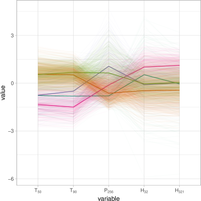
Figure 11: Parallel coordinate plot of 1929 BATSE 4Br GRBs colored as per their group indicators. The solid lines represent the median of the five variables shown in the plot. Variables are in the logarithmic scale.

The five group means of the current analysis are presented in Table 6. In Section 3.1.2 we had used the three parameters duration ($T_{90}$), fluence ($F_{t}$) and hardness ($H_{321}$) to classify the five groups obtained in that section. Such classification is not possible here due to the omission of $F_{t}$. If we are to classify the groups using only the duration variable $T_{90}$, then the fifth group will be classified as the group containing short duration bursts while the first and fourth groups will be classified as the group containing bursts of intermediate duration. The remaining two groups (Groups 2 and 3) are those with the long duration bursts. Comparing the group means of the current analysis with those obtained in the six-parameter analysis (Table 3b) shows good agreement in the case of $\log_{10}H_{32}$ but not for many of the other cases. In general, the second group means are reasonably close for all common parameters. This sort of discrepancy for the other groups and parameters is not very surprising because the exclusion of $\log_{10}F_{t}$ has resulted in less distinct clusters. We facilitate a visual inspection of the five groups obtained in the five-parameters analysis by means of a parallel coordinate plot (Figure 11). Indeed, the medians for many of the parameters are similar to those for the six-parameter case (note that the median is a more robust insensitive measure of the central tendency than the mean) which indicates that the disagreement in the means is perhaps because of the presence of noise owing to the reduced distinctiveness in the five-parameter groupings potentially on account of the exclusion of $\log_{10}F_{t}$.

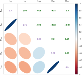
(a) Group 1

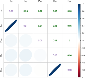
(b) Group 2

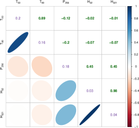
(c) Group 3

(d) Group 4

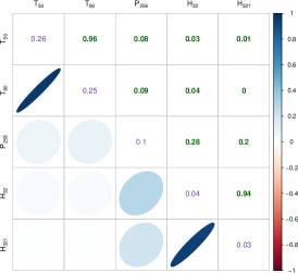
(e) Group 5

Figure 12: Variances and displays of the estimated correlations for each of the five groups obtained by the 5-component GMMBC of the 1929 five-parameter GRBs. For each group, the off-diagonal elements display correlation between the variables while the diagonals display the variances. Both correlations and variances are calculated for the variables in the base-10 logarithmic scale.

We also studied the associations between the five parameters in the five groups. Figure 12 displays the dispersion structures of the five GMMBC groups obtained by GMMBC of the 1929 GRBs. The estimated group variances of the five variables obtained by GMMBC is provided in the diagonals of each display. A very strong positive association is exhibited between the two duration variables ($\log_{10}T_{50}$ and $\log_{10}T_{90}$) and the two hardness ratios ($\log_{10}H_{32}$ and $\log_{10}H_{321}$) for all five groups while $\log_{10}T_{90}$ and $\log_{10}H_{321}$ exhibits a moderate negative association in the first and the fourth groups, a weak negative association in the third group and a weak positive association in the second group. Negligible association is also exhibited between them in the fifth group. On the other hand, $\log_{10}T_{90}$ and $\log_{10}P_{256}$ exhibit a moderately negative association in the first and third groups. In the fourth group they exhibit a moderate positive association and a weak positive association in each of the other two groups. Finally, $\log_{10}P_{256}$ and $\log_{10}H_{321}$ exhibit moderate positive association in the all the groups barring the second one where they show negligible association.

The results of our five-parameter GMMBC analysis on the 1929 GRBs also indicate that there are five kinds of GRBs and reasonable agreement with the groups obtained using the six-parameter analysis with the 1599 GRBs. However, the five-parameter analysis has resulted in less distinct groups owing to the required dropping of $\log_{10}F_{t}$ which was determined to be relevant for GMMBC as per Table 2. It would therefore be important to develop methods which could incorporate missing observations in the analysis. This would permit the inclusion of $\log_{10}F_{t}$ for the 1599 cases for which this information is available in the GMMBC analysis of all the GRBs.

4 Conclusions

Chattopadhyay et al. (2007) carried our $k$-means clustering and GMMBC on the BATSE 4B catalog data and suggested that three classes were adequate to describe the heterogeneity in the GRBs. Other researchers have reported findings of between 2-3 groups of GRBs. These conflicting accounts led us to carry out a detailed review of nonhierarchical clustering methods used in analyzing GRBs from the BATSE 4Br catalog. We found $k$-means to be somewhat inconclusive for clustering GRBs since in our own experiments using $k$-means, the jump statistic, the silhouette index and graphical SPCA projections did not show much support for a few number of homogeneous spherically-dispersed groups. We feel that this may be due to some of the factors involving $k$-means (and clustering algorithms in general). Taking help from a simulated dataset we have reviewed and demonstrated the limitations of $k$-means owing to inherent structural assumptions of the clusters obtained. The variables used by Mukherjee et al. (1998) for non parametric hierarchical clustering and model based clustering is another point of study in this paper. Six variables were used by Chattopadhyay et al. (2007) for their evaluations, but only a subset of these variables have been used by other researchers (Mukherjee et al., 1998; Horváth, 2002; Horváth et al., 2008; Zitouni et al., 2015; Zhang et al., 2016; Veres et al., 2010; Horváth et al., 2010). Mukherjee et al. (1998) eliminated three of the six selected variables citing presence of redundancy among them. Using model-based variable selection, we did not find much evidence of redundancy among the six variables originally selected by Mukherjee et al. (1998). We further perform GMMBC using all the six variables, and used BIC to determine the optimum number of groups and found five homogeneous groups in the BATSE 4Br GRB data. To validate the clustering results obtained through GMMBC, we have calculated the generalized overlap measures which all indicated five distinct groups while modeling GRBs using GMMBC. We thus provide evidence in favor of five groups in the BATSE 4Br dataset using model based clustering. In terms of properties the five groups showed a good degree of resemblance to the three groups obtained by Mukherjee et al. (1998) using model based clustering. Following the procedure of Mukherjee et al. (1998) we have classified the five groups (using duration, fluence and hardness ratios) as intermediate/faint/intermediate, long/intermediate/soft, intermediate/intermediate/intermediate, short/faint/hard and long/bright/intermediate.

Our primary analysis in this paper focused on 1599 GRBs from the BATSE 4Br catalog for which complete information on all the six parameters $\log_{10}T_{50}$, $\log_{10}T_{90}$, $\log_{10}P_{256}$, $\log_{10}H_{32}$, $\log_{10}H_{321}$ and $\log_{10}F_{t}$ were available. All these parameters were determined to be relevant for GMMBC as per variable selection methods. We next analyzed the 1929 GRBs for which complete information is available only on five parameters (i.e., the above six parameters excluding $F_{t}$). Here also, we obtained five distinct groups with good agreement in many of the classifications for the common 1599 GRBs used in both groupings, but the obtained clusters were less distinct in this case. We surmise that this may be on account of the necessity to exclude $F_{t}$ in order to perform GMMBC.

There are a number of issues that could benefit from further attention. For one, the identified groups could be analyzed further in same manner as in Hakkila et al. (2000) or Hakkila et al. (2003). Further, It would be interesting to see if the groupings of GRBs that we have found in this paper are also replicated for datasets from catalogs such as Swift and Fermi. Further, in this paper, we have used only six of the variables available in the BATSE catalog: it would be of interest to see if the unused variables contain additional or more precise information for clustering the GRBs. Further, in this paper, we have followed the standard approach of analyzing the data in the logarithmic scale. It would be of interest to see if more appropriate transformations exist for cluster analysis. Finally, the analysis of the complete BATSE 4Br catalog could benefit further if clustering methods can be developed for use when some of the observations are missing. We feel that GMMBC is particularly well-suited for adaptation in this case because the underlying EM algorithm is originally developed in the context of missing data problems. This would also benefit analysis of other catalogs such as the Swift catalog. Thus, we see that while we have some interesting findings in the context of clustering GRBs, a number of issues meriting further consideration remain.

References

- Akaike (1973) Akaike H., 1973, in Second international symposium on information theory. pp 267–281, doi:10.1007/978-1-4612-1694-0_15
- Akaike (1974) Akaike H., 1974, IEEE Transactions on Automatic Control, 19, 716
- Bagoly et al. (1998) Bagoly Z., Mészáros A., Horváth I., Balázs L. G., Mészáros P., 1998, ApJ, 498, 342
- Baudry et al. (2010) Baudry J.-P., Raftery A. E., Celeux G., Lo K., Gottardo R., 2010, Journal of Computational and Graphical Statistics, 19, 332
- Biernacki et al. (2003) Biernacki C., Celeux G., Govaert G., 2003, Computational Statistics and Data Analysis, 41, 561
- Celeux & Govaert (1992) Celeux G., Govaert G., 1992, Computational Statistics and Data Analysis, 14, 315
- Chang (1983) Chang W. C., 1983, Applied Statistics, 32, 267–275