Simple Length Rigidity for Hitchin Representations

Abstract.

Nous montrons qu’une représentation de Hitchin est déterminée par les rayons spectraux des images de courbes simples et non séparantes. Comme application, nous caractérisons les isométries de la function d’intersection pour les composantes de Hitchin en dimension 3, ainsi que pour les composantes auto-duales en toutes dimensions. Un outil important de notre démonstration est un résultat de transversalité sur les quadruplets positifs de drapeaux.

———————

We show that a Hitchin representation is determined by the spectral radii of the images of simple, non-separating closed curves. As a consequence, we classify isometries of the intersection function on Hitchin components of dimension 3 and on the self-dual Hitchin components in all dimensions. As an important tool in the proof, we establish a transversality result for positive quadruples of flags.

1. Introduction

Any discrete faithful representation of the fundamental group $\pi_{1}(S)$ of a closed oriented surface $S$ of genus greater than 1 into $\mathsf{PSL}_{2}(\mathbb{R})$ is determined, up to conjugacy in $\mathsf{PGL}_{2}(\mathbb{R})$, by the translation lengths of (the images) of a finite collection of elements represented by simple closed curves. More precisely, a collection of $6g-5$ simple closed curves will be enough but $6g-6$ simple closed curve will not suffice, see Schmutz [34] and Hamenstädt [19]. In $\mathsf{PSL}_{2}(\mathbb{R})$ the translation length of an element is determined by the absolute value of the trace (which is well-defined, although the trace is not), so one may equivalently say that a discrete faithful representation of $\pi_{1}(S)$ into $\mathsf{PSL}_{2}(\mathbb{R})$ is determined by the (absolute values of) the traces of a finite collection of elements represented by simple closed curves.

We establish analogues of this result for Hitchin representations. The fact that traces of simple closed curves determine the representation is more surprising in the Hitchin setting as the trace does not even determined the conjugacy class of an element in $\mathsf{PSL}_{d}(\mathbb{R})$ if $d\geqslant 3$.

In the proof, we use Lusztig positivity to establish transversality properties for limit curves of a Hitchin representations, and more generally for positive quadruples of flags. We also establish a rigidity result which depends on correlation functions associated to triples of simple closed curves. We hope that these transversality and rigidity results are of independent interest and that this paper will serve as an introduction to the beautiful algebraic ideas for mathematicians with a more geometric background.

Hitchin representations

A Hitchin representation of dimension $d$ is a representation of $\pi_{1}(S)$ into $\mathsf{PSL}_{d}(\mathbb{R})$ which may be continuously deformed to a $d$-Fuchsian representation that is the composition of the irreducible representation of $\mathsf{PSL}_{2}(\mathbb{R})$ into $\mathsf{PSL}_{d}(\mathbb{R})$ with a discrete faithful representation of $\pi_{1}(S)$ into $\mathsf{PSL}_{2}(\mathbb{R})$. The Hitchin component $\mathcal{H}_{d}(S)$ of all Hitchin representations of $\pi_{1}(S)$ into $\mathsf{PSL}_{d}(\mathbb{R})$, considered up to conjugacy in $\mathsf{PGL}_{d}(\mathbb{R})$, is homeomorphic to $\mathbb{R}^{-(d^{2}-1)\chi(S)}$. In particular, $\mathcal{H}_{2}(S)$ is the Teichmüller space of $S$ – see Section 2 for details and history.

A Hitchin representation is said to be self dual if it is conjugate to its contragredient. Self dual Hitchin representations take values in $\mathsf{PSp}(2n,\mathbb{R})$ and $\mathsf{PSO}(n,n+1)$, when $d=2n$ or $d=2n+1$ respectively. The set $\mathcal{SH}_{d}(S)$ of self dual representations into $\mathsf{PSL}_{d}(\mathbb{R})$ is a contractible submanifold of $\mathcal{H}_{d}(S)$ (see [20]).

Spectrum rigidity

The spectral length of a conjugacy class $\gamma$ in $\pi_{1}(S)$ – or equivalently a free homotopy class of curve in $S$ – with respect to a Hitchin representation $\rho$ is

$$L_{\gamma}(\rho){}\mathrel{\mathop{:}}={}\log\Lambda(\rho(\gamma))$$

where $\Lambda(\rho(\gamma))$ is the spectral radius of $\rho(\gamma)$.

The marked length spectrum of $\rho$ is the function from the set of conjugacy classes in $\pi_{1}(S)$ defined by

$$L(\rho):\gamma\mapsto L_{\gamma}(\rho).$$

Similarly, the marked trace spectrum is the map

$$\gamma\mapsto|\operatorname{Tr}(\rho(\gamma))|,$$

where $|\operatorname{Tr}(A)|$ is the absolute value of the trace of a lift of a matrix $A\in\mathsf{PSL}_{d}(\mathbb{R})$ to $\mathsf{SL}_{d}(\mathbb{R})$.

Our first main result is then

Theorem 1.1.

[Simple Marked Length Rigidity] Two Hitchin representations of a closed orientable surface of genus greater than 2 are equal whenever their marked length spectra coincide on simple non-separating curves.

The restriction on the genus may not only reflect the limit of our methods: we have extended this result to surfaces with boundary, see Section 11, and it is clear that simple length rigidity fails for the pair of pants when $d>2$.

We obtain a finer result for the trace spectrum

Theorem 1.2.

[Simple Marked Trace Rigidity] Two Hitchin representations of a closed orientable surface of genus greater than 2 are equal whenever their marked trace spectra coincide on simple non-separating curves. Furthermore, if $S$ is a closed orientable surface of genus greater than 2 and $d\geqslant 2$, then there exists a finite set $\mathcal{L}_{d}(S)$ of simple non-separating curves, so that two Hitchin representations of $\pi_{1}(S)$ of dimension $d$ are equal whenever their marked trace spectra coincide on $\mathcal{L}_{d}(S)$.

Dal’bo and Kim [12] earlier proved that Zariski dense representations of a group $\Gamma$ into a semi-simple Lie group $\mathsf{G}$ without compact factor are determined, up to automorphisms of $\mathsf{G}$, by the marked spectrum of translation lengths of all elements on the quotient symmetric space $\mathsf{G}/\mathsf{K}$. Similar results were obtained by Charette and Drumm [9] for subgroups of the affine Minkowski group. Bridgeman, Canary, Labourie and Sambarino [7] proved that Hitchin representations, are determined up to conjugacy in $\mathsf{PGL}_{d}(\mathbb{R})$ by the spectral radii of all elements. Bridgeman and Canary [6] proved that discrete faithful representations of $\pi_{1}(S)$ into $\mathsf{PSL}(2,\mathbb{C})$ are determined by the translation lengths of simple non-separating curves on $S$. Duchin, Leininger and Rafi [13] showed that the simple marked length spectrum determines a flat surface, but that no collection of finitely many simple closed curves suffices to determine a flat surface. On the other hand, Marché and Wolff [27, Section 3] gave examples of non-conjugate, indiscrete, non-elementary representations of a closed surface group of genus two into $\mathsf{PSL}_{2}(\mathbb{R})$ with the same simple marked length spectra.

In Section 11 we establish a version of Theorem 1.1 for Hitchin representations of compact surfaces with boundary which are “complicated enough,” while in Section 10 we establish an infinitesimal version of Theorem 1.1.

Isometry groups of the intersection

We apply Theorem 1.1 to characterize diffeomorphisms preserving the intersection function of representations in ${\mathcal{H}}_{d}(S)$.

In Teichmüller theory, the intersection ${\bf I}(\rho,\sigma)$ of representations $\rho$ and $\sigma$ in $\mathcal{T}(S)$ is the length with respect to $\sigma$ of a random geodesic in ${\bf H}^{2}/\rho(\pi_{1}(S))$ – where ${\bf H}^{2}$ is the hyperbolic plane. Thurston showed that the Hessian of the intersection function gives rise to a Riemannian metric on $\mathcal{T}(S)$, which Wolpert [35] showed was a multiple of the classical Weil–Petersson metric – see also Bonahon [3], McMullen [30], and Bridgeman [5] for further interpretation. As a special case of their main result, Bridgeman, Canary, Labourie and Sambarino [7] used the Hessian of a renormalized intersection function to construct a mapping class group invariant, analytic, Riemannian metric on ${\mathcal{H}}_{d}(S)$, called the pressure metric – see Section 8 for details.

Royden [32] showed that the isometry group of $\mathcal{T}(S)$, equipped with the Teichmüller metric, is the extended mapping class group, while Masur and Wolf [29] established the same result for the Weil–Petersson metric.

In our context, the intersection isometry group – respectively self dual intersection isometry group– is the set of those diffeomorphisms of $\mathcal{H}_{d}(S)$ – respectively $\mathcal{SH}_{d}(S)$ – preserving ${\bf I}$.

Theorem 1.3.

[Self dual isometry group] For a surface of genus greater than 2, the self dual intersection isometry group coincides with the extended mapping class group of $S$.

We have a finer result when $d=3$.

Theorem 1.4.

[Isometry Group In Dimension 3] For a surface $S$ of genus greater than 2, the intersection isometry group of $\mathcal{H}_{3}(S)$ is generated by the extended mapping class group of $S$ and the contragredient involution.

Since, as we will see in the proof, isometries of the intersection function are also isometries of the pressure metric, we view this as evidence for the conjecture that this is also the isometry group of the pressure metric – See Section 8.1 for precise definitions.

Our proof follows the outline suggested by the proof in Bridgeman–Canary [6] that the isometry group of the intersection function on quasifuchsian space is generated by the extended mapping class group and complex conjugation.

A key tool in the proof of Theorem 1.4 is a rigidity result for the marked simple, non-separating Hilbert length spectrum for a representation into $\mathsf{PSL}(3,\mathbb{R})$, see Section 9. Kim [21], see also Cooper-Delp [11], had previously proved a marked Hilbert length rigidity theorem for the full marked length spectrum.

Positivity and correlation functions

Every element of the image of a Hitchin representation is purely loxodromic, i.e. diagonalizable with real eigenvalues of distinct modulus. We introduce correlation functions which record the relative positions of eigenspaces of elements in the image and give rise to a rigidity result for the restrictions of Hitchin representation to certain three generator subgroups. This new rigidity result relies crucially on a new transversality result for eigenbases of images of disjoint curves.

If $\rho$ is a Hitchin representation of dimension $d$, and $\gamma$ is a non-trivial element, a matrix representing $\rho(\gamma)$ may be written –see Section 2 – as

$$\rho(\gamma)=\sum_{i=1}^{d}\lambda_{i}\left(\rho(\gamma)\right){\bf{p}}_{i}\left(\rho(\gamma)\right),$$

where $\lambda_{1}\left(\rho(\gamma)\right)>\ldots>\lambda_{d}\left(\rho(\gamma)\right)>0$ are the eigenvalues (of some lift) of $\rho(\gamma)$ and ${\bf{p}}_{i}\left(\rho(\gamma)\right)$ are the projectors onto the corresponding 1-dimensional eigenspaces. Let

• $\mathcal{A}=(\alpha_{1},\ldots,\alpha_{n})$ be an $n$-tuple of non-trivial elements of $\pi_{1}(S)$,

• $I=\left(i_{j}\right)_{j\in\{1,\ldots,n\}}$ be an $n$-tuple of elements in $\{1,\ldots,d\}$.

The associated correlation function ${\bf T}_{I}(\mathcal{A})$ on $\mathcal{H}_{d}(S)$ is defined by

$${\bf T}_{I}(\mathcal{A}):\rho\mapsto\operatorname{Tr}\left(\prod_{j=1}^{n}{\bf{p}}_{i_{j}}(\rho(\alpha_{j}))\right).$$

We show that finitely many of these correlation often suffice to determine the restriction of a Hitchin representation to a three generator subgroup. One may use this result to give an embedding of $\mathcal{H}_{d}(S)$ in some $\mathbb{R}^{N}$ and we hope that a refinement of these ideas could yield new parametrisations of $\mathcal{H}_{d}(S)$. In the statement below, recall that a pair of disjoint simple closed curves is said to be non-parallel if they do not bound an annulus.

Theorem 1.5.

[Rigidity for correlations functions] Let $\rho$ and $\sigma$ be Hitchin representations in $\mathcal{H}_{d}(S)$. Suppose that $\alpha,\beta,\delta\in\pi_{1}(S)-\{1\}$ are represented by based loops which are freely homotopic to a collection of pairwise disjoint and non-parallel simple closed curves. Assume that

1. for any $\eta\in\{\alpha,\beta,\delta\}$, $\rho(\eta)$ and $\sigma(\eta)$ have the same eigenvalues,

2. for all $i,j,k$ in $\{1,\ldots,d\}$

   $$\frac{{\bf T}_{i,j,k}(\alpha,\beta,\delta)}{{\bf T}_{j,k}(\beta,\delta)}(\rho)=\frac{{\bf T}_{i,j,k}(\alpha,\beta,\delta)}{{\bf T}_{j,k}(\beta,\delta)}(\sigma),$$

then $\rho$ and $\sigma$ are conjugate, in $\mathsf{PGL}_{d}(\mathbb{R})$, on the subgroup of $\pi_{1}(S)$ generated by $\alpha$, $\beta$ and $\gamma$.

Before even stating that theorem, we need to prove the relevant correlation functions never vanish. This will be a corollary of the following theorem. First recall that a Hitchin representation in $\mathcal{H}_{d}(S)$ defines a limit curve in the flag manifold of $\mathbb{R}^{d}$, so that any two distinct points are transverse. Recall also that any transverse pair flags $a$ and $b$ in $\mathbb{R}^{d}$ defines a decomposition of $\mathbb{R}^{d}$ into a sum of $d$ lines $L_{1}(a,b),\ldots L_{d}(a,b)$.

Theorem 1.6.

[Transverse bases] Let $\rho$ be a Hitchin representation of dimension $d$. Let $(a,x,y,b)$ be four cyclically ordered points in the limit curve of $\rho$, then any $d$ lines in

$$\{L_{1}(a,b),\ldots,L_{d}(a,b),L_{1}(x,y),\ldots,L_{d}(x,y)\}$$

are in general position.

This last result is a consequence of the positivity theory developed by Lusztig [25] and used in the theory of Hitchin representations by Fock–Goncharov [14] and is actually a special case of a more general result about positive quadruples, see Theorem 3.6. Theorem 3.6 may be familiar to experts but we could not find a proper reference to it in the literature.

We also establish a more general version of Theorem 1.5, see Theorem 4.4.

Structure of the proof

Let us sketch the proof of Theorem 1.1. The proof runs through the following steps. We first show, in Section 6, that if the length spectra agree on simple non-separating curves, then all the eigenvalues agree for these curves. This follows by considering curves of the form $\alpha^{n}\beta$ when $\alpha$ and $\beta$ have geometric intersection one and using an asymptotic expansion. A similar argument yields that ratio of correlation functions agree for certain triples of curves that only exist in genus greater than 2, see Theorem 7.1, and a repeated use of Theorem 1.5 concludes the proof of Theorem 1.1. Theorem 1.6 is crucially used several times to show that coefficients appearing in asymptotic expansions do not vanish.

Acknowledgements

Section 3 uses ideas that are being currently developed by the third author in collaboration with Olivier Guichard and Anna Wienhard. We have benefitted immensely from discussions with Yves Benoist, Sergey Fomin, Olivier Guichard, Andres Sambarino and Anna Wienhard and wish to thank them here. This material is partially based upon work supported by the National Science Foundation while the third author was in residence at the Mathematical Sciences Research Institute in Berkeley, CA, during the Fall 2016 semester. The authors also gratefully acknowledge support from U.S. National Science Foundation grants DMS 1107452, 1107263, 1107367 "RNMS: GEometric structures And Representation varieties" (the GEAR Network).

2. Hitchin representations and limit maps

2.1. Definitions

Let $S$ be a closed orientable surface of genus $g\geqslant 2$. A representation $\rho:\pi_{1}(S)\to\mathsf{PSL}_{2}(\mathbb{R})$ is said to be Fuchsian if it is discrete and faithful. Recall that Teichmüller space $\mathcal{T}(S)$ is the subset of

$${\rm Hom}(\pi_{1}(S),\mathsf{PSL}_{2}(\mathbb{R}))/\mathsf{PGL}_{2}(\mathbb{R})$$

consisting of (conjugacy classes of) Fuchsian representations.

Let $\tau_{d}:\mathsf{PSL}_{2}(\mathbb{R})\to\mathsf{PSL}_{d}(\mathbb{R})$ be the irreducible representation (which is well-defined up to conjugacy). A representation $\sigma:\pi_{1}(S)\to\mathsf{PSL}_{d}(\mathbb{R})$ is said to be $d$-Fuchsian if it has the form $\tau_{d}\circ\rho$ for some Fuchsian representation $\rho:\pi_{1}(S)\to\mathsf{PSL}_{2}(\mathbb{R})$. A representation $\sigma:\pi_{1}(S)\to\mathsf{PSL}_{d}(\mathbb{R})$ is a Hitchin representation if it may be continuously deformed to a $d$-Fuchsian representation. The Hitchin component ${\mathcal{H}}_{d}(S)$ is the component of the space of reductive representations up to conjugacy:

$${\rm Hom}^{\operatorname{red}}(\pi_{1}(S),\mathsf{PSL}_{d}(\mathbb{R}))/\mathsf{PGL}_{d}(\mathbb{R})$$

consisting of (conjugacy classes of) Hitchin representations. In analogy with Teichmüller space $\mathcal{T}(S)=\mathcal{H}_{2}(S)$, Hitchin proved that ${\mathcal{H}}_{d}(S)$ is a real analytic manifold diffeomorphic to a cell.

Theorem 2.1.

(Hitchin [20]) If $S$ is a closed orientable surface of genus $g\geqslant 2$ and $d\geqslant 2$, then ${\mathcal{H}}_{d}(S)$ is a real analytic manifold diffeomorphic to $\mathbb{R}^{(d^{2}-1)(2g-2)}$.

The Fuchsian locus is the subset of ${\mathcal{H}}_{d}(S)$ consisting of $d$-Fuchsian representations. It is naturally identified with $\mathcal{T}(S)$.

2.2. Real-split matrices and proximality

If $A\in\mathsf{SL}_{d}(\mathbb{R})$ is real-split, i.e. diagonalizable over $\mathbb{R}$, we may order the eigenvalues $\{\lambda_{i}(A)\}_{i=1}^{d}$ so that

$$|\lambda_{1}(A)|\geqslant|\lambda_{2}(A)|\geqslant\cdots|\lambda_{d-1}(A)|\geqslant|\lambda_{d}(A)|.$$

Let $\{e_{i}(A)\}_{i=1}^{d}$ be a basis for $\mathbb{R}^{d}$ so that $e_{i}(A)$ is an eigenvector with eigenvalue $\lambda_{i}(A)$ and let $e^{i}(A)$ denote the linear functional so that $\braket{e^{i}(A)}{e_{i}(A)}=1$ and $\braket{e^{i}(A)}{e_{j}(A)}=0$ if $i\neq j$. Let ${\bf{p}}_{i}(A)$ denote the projection onto $\braket{e_{i}(A)}$ parallel to the hyperplane spanned by the other $d-1$ basis elements. Then,

$${\bf{p}}_{i}(A)(v)=\braket{e^{i}(A)\ }{\ v}\ e_{i}(A)$$

and we may write

$$A=\sum_{i=1}^{d}\lambda_{i}(A){\bf{p}}_{i}(A).$$

We say that $A$ is $k$-proximal if

$$|\lambda_{1}(A)|>|\lambda_{2}(A)|>\ldots|\lambda_{k}(A)|>|\lambda_{k+1}(A)|$$

and we say that $A$ is purely loxodromic if it is $(d-1)$-proximal, in which case it is diagonalizable over $\mathbb{R}$ with eigenvalues of distinct modulus. If $A$ is $k$-proximal, then, for all $i=1,\ldots,k$, ${\bf{p}}_{i}(A)$ is well-defined and $e_{i}(A)$ is well-defined up to scalar multiplication. Moreover, if $A$ is purely loxodromic ${\bf{p}}_{i}(A)$ is well-defined and $e_{i}(A)$ and $e^{i}(A)$ are well-defined up to scalar multiplication for all $i$. If $A\in\mathsf{PSL}_{d}(\mathbb{R})$, we say that $A$ is purely loxodromic if any lift of $A$ to an element of $\mathsf{SL}_{d}(\mathbb{R})$ is purely loxodromic.

2.3. Transverse flags and associated bases

A flag for $\mathbb{R}^{d}$ is a nested family

$$f=(f^{1},f^{2},\ldots,f^{d-1})$$

of vector subspaces of $\mathbb{R}^{d}$ where $f^{i}$ has dimension $i$ and $f^{i}\subset f^{i+1}$ for each $i$. Let $\mathcal{F}_{d}$ denote the space of all flags for $\mathbb{R}^{d}$. An $n$-tuple $(f_{1},\ldots,f_{n})\in\mathcal{F}_{d}^{n}$ is transverse if

$$f^{d_{1}}_{1}\oplus f^{d_{2}}_{2}\oplus\ldots\oplus f^{d_{n}}_{n}=\mathbb{R}^{d}$$

for any partition $\{d_{i}\}_{i\in\{1,\ldots,n\}}$ of $d$. Let $\mathcal{F}_{d}^{(n)}$ be the set of transverse $n$-tuples of flags, and note that $\mathcal{F}_{d}^{(n)}$is an open dense subset of $\mathcal{F}_{d}^{n}$.

Two transverse flags $(a,b)$ determine a decomposition of $\mathbb{R}^{d}$ as sum of lines $\{L_{i}(a,b)\}_{i=1}^{d}$ where

$$L_{i}(a,b)=a^{i}\cap b^{d-i+1}$$

for all $i$. A basis $\varepsilon^{a}_{b}=\{e_{i}\}$ for $\mathbb{R}^{d}$ is consistent with $(a,b)\in\mathcal{F}_{d}^{(2)}$ if $e_{i}\in L_{i}(a,b)$ for all $i$, or, equivalently, if

$$a^{j}=\braket{e_{1},\ldots,e_{j}}\quad{\rm and}\quad b^{j}=\braket{e_{d},\ldots,e_{d-j+1}}$$

for all $j$. In particular, the choice of basis is well-defined up to scalar multiplication of basis elements.

2.4. Limit maps

Labourie [22] associates a limit map from $\partial_{\infty}\pi_{1}(S)$ into $\mathcal{F}_{d}$ to every Hitchin representation. This map encodes many crucial properties of the representation.

Theorem 2.2.

(Labourie [22]) If $\rho\in{\mathcal{H}}_{d}(S)$, then there exists a unique continuous $\rho$-equivariant map $\xi_{\rho}:\partial_{\infty}\pi_{1}(S)\rightarrow{\mathcal{F}}_{d}$, such that:

1. (Proximality) If $\gamma\in\pi_{1}(S)-\{1\}$, then $\rho(\gamma)$ is purely loxodromic and

   $$\xi_{\rho}^{i}(\gamma^{+})=\braket{e_{1}(\rho(\gamma)),\ldots,e_{i}(\rho(\gamma))}$$

   for all $i$, where $\gamma^{+}\in\partial_{\infty}\pi_{1}(S)$ is the attracting fixed point of $\gamma$.

2. (Hyperconvexity) If $x_{1},\ldots,x_{k}\in\partial_{\infty}\pi_{1}(S)$ are distinct and $m_{1}+\ldots+m_{k}=d$, then

   $$\xi^{m_{1}}(x_{1})\oplus\ldots\oplus\xi^{m_{j}}(x_{j})\oplus\ldots\oplus\xi^{m_{k}}(x_{k})=\mathbb{R}^{d}.$$

Notice that if $\gamma\in\pi_{1}(S)-\{1\}$ and $\gamma^{\pm}\in\partial_{\infty}\pi_{1}(S)$ are its attracting and repelling fixed points, then $\rho(\gamma)$ is diagonal with respect to any basis consistent with $(\xi_{\rho}(\gamma^{+}),\xi_{\rho}(\gamma^{-}))$. Moreover, if $\sigma$ is in the Fuchsian locus, then $\sigma(\gamma)$ has a lift to $\mathsf{SL}_{d}(\mathbb{R})$ all of whose eigenvalues are positive. Therefore, if $\rho\in{\mathcal{H}}_{d}(S)$, then $\rho(\gamma)$ has a lift to $\mathsf{SL}_{d}(\mathbb{R})$ with positive eigenvalues and we define

$$\lambda_{1}(\rho(\gamma))>\lambda_{2}(\rho(\gamma))>\cdots>\lambda_{d}(\rho(\gamma))>0$$

to be the eigenvalues of this specific lift.

It will also be useful to note that any Hitchin representation $\rho:\pi_{1}(S)\rightarrow\mathsf{PSL}_{d}(\mathbb{R})$ can be lifted to a representation $\tilde{\rho}:\pi_{1}(S)\to\mathsf{SL}_{d}(\mathbb{R})$. Moreover, Hitchin [20, Section 10] observed that every Hitchin component lifts to a component of ${\rm Hom}^{\operatorname{red}}(\pi_{1}(S),\mathsf{SL}_{d}(\mathbb{R}))/\mathsf{SL}_{d}(\mathbb{R})$.

2.5. Other Lie groups and other length functions

More generally, if $\mathsf{G}$ is a split, real simple adjoint Lie group, Hitchin [20] studies the component

$$\mathcal{H}(S,\mathsf{G})\subset{\rm Hom}^{\operatorname{red}}(\pi_{1}(S),\mathsf{G})/\mathsf{G}$$

which contains the composition of a Fuchsian representation into $\mathsf{PSL}_{2}(\mathbb{R})$ with an irreducible representation of $\mathsf{PSL}_{2}(\mathbb{R})$ into $\mathsf{G}$ and shows that it is an analytic manifold diffeomorphic to $\mathbb{R}^{(2g-2){\rm dim}(\mathsf{G})}$.

If $\rho\in{\mathcal{H}}_{d}(S)$, then we define the contragredient representation $\rho^{*}\in{\mathcal{H}}_{d}(S)$ by $\rho^{*}(\gamma)=\rho(\gamma^{-1})^{T}$ for all $\gamma\in\pi_{1}(S)$. The contragredient involution of ${\mathcal{H}}_{d}(S)$ takes $\rho$ to $\rho^{*}$.

We define the self dual Hitchin representations – and accordingly the self dual Hitchin component $\mathcal{S}{\mathcal{H}}_{d}(S)$ – to be the fixed points of the contragredient involution. Since the contragredient involution is an isometry of the pressure metric, $\mathcal{S}{\mathcal{H}}_{d}(S)$ is a totally geodesic submanifold of ${\mathcal{H}}_{d}(S)$.

Observe then that if $\rho$ is a self dual Hitchin representation and $\gamma\in\pi_{1}(S)$, then the eigenvalues $\lambda_{1}(\rho(\gamma)),\ldots,\lambda_{d}(\rho(\gamma))$ satisfy $\lambda_{i}^{-1}(\rho(\gamma))=\lambda_{d-i+1}(\rho(\gamma))$ for all $i$. On the other hand, Theorem 1.2 in [7] implies that if $\lambda_{1}^{-1}(\rho(\gamma))=\lambda_{d}(\rho(\gamma))$ for all $\gamma$, then $\rho$ is conjugate to its contragredient $\rho^{*}$. Notice that the contragredient involution fixes each point in $\mathcal{H}(S,\mathsf{PSp}(2d,\mathbb{R}))$, $\mathcal{H}(S,\mathsf{PSO}(d,d+1))$, and $\mathcal{H}(S,\mathsf{G}_{2,0})$ considered as subsets of $\mathcal{H}(S,\mathsf{PSL}(2d,\mathbb{R}))$, $\mathcal{H}(S,\mathsf{PSL}(2d+1,\mathbb{R}))$, and $\mathcal{H}(S,\mathsf{PSL}(7,\mathbb{R}))$ respectively. Conversely, a self dual representation, being conjugate to its contragredient, is not Zariski dense, hence belongs to such a subset by a result of Guichard [17]. In particular, $\mathcal{S}\mathcal{H}_{2d}(S)=\mathcal{H}(S,\mathsf{PSp}(2d,\mathbb{R}))$ and $\mathcal{S}\mathcal{H}_{2d+1}(S)=\mathcal{H}(S,\mathsf{PSO}(d,d+1))$.

In our work on isometries of the intersection function, it will be useful to consider the Hilbert length $L_{\gamma}^{H}(\rho)$ of $\rho(\gamma)$ when $\gamma\in\pi_{1}(S)$ and $\rho\in{\mathcal{H}}_{d}(S)$, where

$$L_{\gamma}^{H}(\rho) {}\mathrel{\mathop{:}}={} \log\lambda_{1}(\rho(\gamma))-\log\lambda_{d}(\rho(\gamma))\ ,$$

and similarly the Hilbert length spectrum as a function on free homotopy classes. Notice that $L^{H}_{\gamma}(\rho)=L^{H}_{\gamma^{-1}}(\rho)=L^{H}_{\gamma}(\rho^{*})$. One readily observes that a representation is self dual if and only if $L^{H}_{\gamma}(\rho)=2L_{\gamma}(\rho)$ for all non-trivial $\gamma\in\pi_{1}(S)$.

3. Transverse bases

In this section, we prove a strong transversality property for ordered quadruples of flags in the limit curve of a Hitchin representation, which we regard as a generalization of the hyperconvexity property established by Labourie [22] (see Theorem 2.2). (Recall that any pair $(a,b)$ of transverse flags determines a decomposition of $\mathbb{R}^{d}$ into a sum of $d$ lines $L_{1}(a,b)\oplus\cdots\oplus L_{d}(a,b)$ where $L_{i}(a,b)=a^{i}\cap b^{d-i+1}$.)

Theorem 1.6. Let $\rho$ be a Hitchin representation of dimension $d$ and let $(a,x,y,b)$ be four cyclically ordered points in the limit curve of $\rho$, then any $d$ lines in

$$\{L_{1}(a,b),\ldots,L_{d}(a,b),L_{1}(x,y),\ldots,L_{d}(x,y)\}$$

are in general position.

The proof of Theorem 1.6 relies on the theory of positivity developed by Lusztig [25] and applied to representations of surface groups by Fock and Goncharov [14]. It will follow from a more general result for positive quadruples of flags, see Theorem 3.6.

Remark: When $\rho\in\mathcal{H}_{3}(S)$, there exists a strictly convex domain $\Omega_{\rho}$ in $\mathbb{RP}^{2}$ with $C^{1}$ boundary so that $\rho(\pi_{1}(S))$ acts properly discontinuously and cocompactly on $\Omega_{\rho}$, see Benoist [2] and Choi-Goldman [10]. If $\xi_{\rho}$ is the limit map of $\rho$, then $\xi_{\rho}^{1}$ identifies $\partial_{\infty}\pi_{1}(S)$ with $\partial\Omega_{\rho}$, while $\xi_{\rho}^{2}(z)$ is the plane spanned by the (projective) tangent line to $\partial\Omega_{\rho}$ at $\xi_{\rho}^{1}(z)$. In this case, Theorem 1.6 is an immediate consequence of the strict convexity of $\Omega_{\rho}$, since if $x$ and $y$ lie in the limit curve, then $L_{1}(x,y)=x^{1}$, $L_{3}(x,y)=y^{1}$ and $L_{2}(x,y)$ is the intersection of the tangent lines to $\Omega_{\rho}$ at $x^{1}$ and $y^{1}$. Moreover, one easily observes that the analogue of Theorem 1.6 does not hold for cyclically ordered quadruples of the form $(a,x,b,y)$.

3.1. Components of positivity

Given a flag $a$, we define the Schubert cell $B_{a}\subset\mathcal{F}_{d}$ to be the set of all flags transverse to $a$. Let $U_{a}$ be the group of unipotent elements in the stabilizer of $a$, i.e. the set of unipotent upper triangular matrices with respect to a basis $\{e_{i}\}$ consistent with $a$. If $b\in B_{a}$, we can assume that $\{e_{i}\}$ is consistent with $(a,b)$, so it is apparent that the stabilizer of $b$ in $U_{a}$ is trivial. The lemma below follows easily.

Lemma 3.1.

If $b\in B_{a}$, then $B_{a}=U_{a}(b)$. Moreover, the map

$$h_{b}:U_{a}\to B_{a}$$

defined by $h_{b}(u)=u(b)$ is a diffeomorphism.

Suppose that $(a,b)\in\mathcal{F}_{d}^{(2)}$ and $\varepsilon^{a}_{b}$ is a basis consistent with the pair $(a,b)$. Recall that $A\in\mathsf{SL}_{d}(\mathbb{R})$ is totally positive with respect to $\varepsilon^{a}_{b}$, if every minor in its matrix with respect to the basis $\varepsilon^{a}_{b}$ is positive. Similarly, we say that $A\in\mathsf{SL}_{d}(\mathbb{R})$ is totally non-negative with respect to $\varepsilon^{a}_{b}$, if every minor in its matrix with respect to the basis $\varepsilon^{a}_{b}$ is non-negative. Let $U(\varepsilon^{a}_{b})_{\geqslant 0}\subset U_{a}$ be the set of totally non-negative unipotent upper triangular matrices with respect to $\varepsilon^{a}_{b}$. We say that a minor is an upper minor with respect to $\varepsilon^{a}_{b}$ if it is non-zero for some element of $U(\varepsilon^{a}_{b})_{\geqslant 0}$. We then let $U(\varepsilon^{a}_{b})_{>0}$ be the subset of $U(\varepsilon^{a}_{b})_{\geqslant 0}$ consisting of elements all of whose upper minors with respect to $\varepsilon^{a}_{b}$ are positive. Moreover, let $\Delta(\varepsilon^{a}_{b})_{>0}$ be the group of matrices which are diagonalizable with respect to $\varepsilon^{a}_{b}$ with positive eigenvalues. Lusztig [25] proves that

Lemma 3.2.

(Lusztig [25, Sec. 2.12, Sec. 5.10] If $(a,b)\in\mathcal{F}_{d}^{(2)}$ and $\varepsilon^{a}_{b}$ is a basis consistent with the pair $(a,b)$, then

$$U(\varepsilon^{a}_{b})_{\geqslant 0}U(\varepsilon^{a}_{b})_{>0}\subset U(\varepsilon^{a}_{b})_{>0}\quad\textrm{and}\quad\overline{U(\varepsilon^{a}_{b})_{>0}}=U(\varepsilon^{a}_{b})_{\geqslant 0}\subset U_{a}.$$

If $i\neq j$ and $t\in\mathbb{R}$, the elementary Jacobi matrix $J_{ij}(t)$ with respect to $\varepsilon^{a}_{b}=\{e_{i}\}$ is the matrix such that $J_{ij}=e_{j}+te_{i}$ and $J_{ij}(e_{k})=e_{k}$ if $k\neq i$. If $i<j$ and $t>0$, then $J_{ij}(t)\in U(\varepsilon^{a}_{b})_{\geqslant 0}$. Moreover, $U(\varepsilon^{a}_{b})_{\geqslant 0}$ is generated by elementary Jacobi matrices of this form (see, for example, [15, Thm. 12]). So,

1. the semigroup $U(\varepsilon^{a}_{b})_{\geqslant 0}$ is connected, and

2. if $g\in\Delta(\varepsilon^{a}_{b})$, then $gU(\varepsilon^{a}_{b})_{>0}g^{-1}=U(\varepsilon^{a}_{b})_{>0}$.

We define the component of positivity for $\varepsilon^{a}_{b}$ as

$$V(\varepsilon^{a}_{b}){}\mathrel{\mathop{:}}={}U(\varepsilon^{a}_{b})_{>0}(b).$$

Lusztig [25, Thm. 8.14] (see also Lusztig [26, Lem. 2.2]) identifies $V(\varepsilon^{a}_{b})$ with a component of the intersection $B_{a}\cap B_{b}$ of two opposite Schubert cells.

Lemma 3.3.

(Lusztig [25, Thm. 8.14]) If $(a,b)\in\mathcal{F}_{d}^{(2)}$ and $\varepsilon^{a}_{b}$ is a basis consistent with the pair $(a,b)$, then $V(\varepsilon^{a}_{b})$ is a connected component of $B_{a}\cap B_{b}$.

3.2. Positive configurations of flags

We now recall the theory of positive configurations of flags as developed by Fock and Goncharov [14].

A triple $(a,x,b)\in\mathcal{F}_{d}^{(3)}$ is positive with respect to a basis $\varepsilon^{a}_{b}$ consistent with $(a,b)$ if $x=u(b)$ for some $u\in U(\varepsilon^{a}_{b})_{>0}$. If $x\in V(\varepsilon^{a}_{b})$, we define

$$V(a,x,b)=V(\varepsilon^{a}_{b})$$

and notice that $V(a,x,b)$ is the component of $B_{a}\cap B_{b}$ which contains $x$.

More generally, a $(n+2)$-tuple $(a,x_{n},\ldots,x_{1},b)\in\mathcal{F}_{d}^{(n+2)}$ of flags is positive if there exist $u_{i}\in U(\varepsilon^{a}_{b})_{>0}$ so that $x_{p}=u_{1}\cdots u_{p}(b)$ for all $p$. By construction, the set of positive $(n+2)$-tuples of flags is connected. Since $U(\varepsilon^{a}_{b})_{>0}$ is a semi-group, $(a,x_{i},b)$ is a positive triple for all $i$ and, more generally, $(a,x_{i_{1}},\ldots,x_{i_{k}},b)$ is a positive $(k+2)$-tuple whenever $1\leqslant i_{i}<\cdots<i_{k}\leqslant n$.

Fock and Goncharov showed that the positivity of a $n$-tuple is invariant under the action of the dihedral group on $n$ elements.

Proposition 3.4.

(Fock-Goncharov [14, Thm. 1.2]) If $(a_{1},\ldots,a_{n})$ is a positive $n$-tuple of flags in $\mathcal{F}_{d}$, then $(a_{2},a_{3},\ldots,a_{n},a_{1})$ and $(a_{n},a_{n-1},\ldots,a_{1})$ are both positive as well.

As a consequence, we see that every sub $k$-tuple of a positive $n$-tuple is itself positive.

Corollary 3.5.

If $(a_{1},\ldots,a_{n})$ is a positive $n$-tuple of flags in $\mathcal{F}_{d}$ and $1\leqslant i_{1}<i_{2}<\cdots<i_{k}\leqslant n$, then $(a_{i_{1}},a_{i_{2}},\ldots,a_{i_{k}})$ is positive.

Proof.

It suffices to prove that every sub $(n-1)$-tuple of a positive $n$-tuple is positive. By Proposition 3.4, we may assume that the sub $(n-1)$-tuple has the form $(a_{1},a_{3},\ldots,a_{n})$ and we have already seen that this $(n-1)$-tuple is positive. ∎

The main result of the section can now be formulated more generally as a result about positive quadruples. Its proof will be completed in Section 3.7.

Theorem 3.6.

[Transverse bases for quadruples] Let $(a,x,y,b)$ be a positive quadruple in $\mathcal{F}_{d}$, then any $d$ lines in

$$\{L_{1}(a,b),\ldots,L_{d}(a,b),L_{1}(x,y),\ldots,L_{d}(x,y)\}$$

are in general position.

3.3. Positive maps

If $\Sigma$ is a cyclically ordered set with at least 4 elements, a map $\gamma:\Sigma\to\mathcal{F}_{d}$ is said to be positive if whenever $(z_{1},z_{2},z_{3},z_{4})$ is an ordered quadruple in $\Sigma$, then its image $(\gamma(z_{1}),\gamma(z_{2}),\gamma(z_{3}),\gamma(z_{4}))$ is a positive quadruple in $\mathcal{F}_{d}^{(4)}$.

For example, given an irreducible representation

$$\tau_{d}:\mathsf{PSL}_{2}(\mathbb{R})\to\mathsf{PSL}_{d}(\mathbb{R})$$

the $\tau_{d}$-equivariant Veronese embedding

$$\nu_{\tau}:\partial{\bf H}^{2}={\bf P}^{1}(\mathbb{R})\to\mathcal{F}_{d}$$

(where $\nu_{\tau}$ takes the attracting fixed point of $g\in\mathsf{PSL}_{2}(\mathbb{R})$ to the attracting fixed point of $\tau_{d}(g)$) is a positive map. More generally, Fock and Goncharov, see also Labourie-McShane [23, Appendix B], showed that the limit map of a Hitchin representation is positive.

Theorem 3.7.

(Fock-Goncharov [14, Thm 1.15]) If $\rho\in{\mathcal{H}}_{d}(S)$, then the associated limit map $\xi_{\rho}:\partial_{\infty}\pi_{1}(S)\rightarrow{\mathcal{F}}_{d}$ is positive.

Notice that Theorem 1.6 follows immediately from Theorems 3.6 and 3.7.

We observe that one may detect the positivity of a $n$-tuple using only quadruples, which immediately implies that positive maps take cyclically ordered subsets to positive configurations.

Lemma 3.8.

If $n\geqslant 2$, then an $(n+2)$-tuple $(a,x_{n},\ldots,x_{1},b)$ is positive if and only if $(a,x_{i+1},x_{i},b)$ is positive for all $i=1,\ldots,n-1$.

Proof.

Corollary 3.5 implies that if $(a,x_{n},\ldots,x_{1},b)$ is positive, then $(a,x_{i+1},x_{i},b)$ is positive for all $i$.

Now suppose that $(a,x_{i+1},x_{i},b)$ is positive for all $i=1,\ldots,n-1$. Since $(a,x_{2},x_{1},b)$ is positive, there exists $u_{1},u_{2}\in U(\varepsilon^{a}_{b})_{>0}$ so that $x_{1}=u_{1}(b)$ and $x_{2}=u_{1}u_{2}(b)$. If we assume that there exists $u_{i}\in U(\varepsilon^{a}_{b})_{>0}$, for all $i\leqslant k<n$, so that $x_{p}=u_{1}\cdots u_{p}(b)$ for all $p\leqslant k$, then, since $(a,x_{k+1},x_{k},b)$ is positive, there exists $u_{k+1},v_{k}\in U(\varepsilon^{a}_{b})_{>0}$ such that $x_{k+1}=v_{k}u_{k+1}(b)$ and $x_{k}=v_{k}(b)$. However, Lemma 3.1 implies that $v_{k}=u_{1}\cdots u_{k}$. Iteratively applying this argument, we see that $(a,x_{n},\ldots,x_{1},b)$ is positive. ∎

Corollary 3.9.

If $\Sigma$ is a cyclically ordered set, $f:\Sigma\to\mathcal{F}_{d}$ is a positive map and $(a_{1},\ldots,a_{n})$ is a cyclically ordered $n$-tuple in $\Sigma$, then $(f(a_{1}),f(a_{2}),f(a_{3}),\ldots,f(a_{n}))$ is a positive $n$-tuple in $\mathcal{F}_{d}$.

The following result allows one to simplify the verification that a map of a finite set into ${\mathcal{F}}_{d}$ is positive, see also Section 5.11 in Fock-Goncharov [14]

Proposition 3.10.

Let $P$ be a finite set in $\partial_{\infty}{\bf H}^{2}$ and $\mathcal{T}$ be an ideal triangulation of the convex polygon spanned by $P$. A map $f:P\to\mathcal{F}_{d}$ is positive if whenever $(x,y,z,w)$ are the (cyclically ordered) vertices of two ideal triangles in $\mathcal{T}$ which share an edge, then $(f(x),f(y),f(z),f(w))$ is a positive quadruple.

Proof.

Suppose $\mathcal{T}^{\prime}$ is obtained from $\mathcal{T}$ by replacing an internal edge of $\mathcal{T}$ by an edge joining the opposite vertices of the adjoining triangles. In this case, we say that $\mathcal{T}^{\prime}$ is obtained from $\mathcal{T}$ by performing an elementary move. Label the vertices of the original edge by $a$ and $b$ and the vertices of the new edge by $x$ and $y$, so that the vertices occur in the order $(a,x,b,y)$ in $\partial_{\infty}{\bf H}^{2}$. If the edge $(y,a)$ abuts another triangle with additional vertex $z$, then $(a,x,y,z)$ is a cyclically ordered collection of points in $P$ which are the vertices of two ideal triangles in $\mathcal{T}^{\prime}$ which share an edge. By our original assumption on $\mathcal{T}$, $(f(a),f(x),f(b),f(y))$ and $(f(a),f(b),f(y),f(z))$ are positive, so, by Proposition 3.4, $(f(y),f(a),f(x),f(b))$ and $(f(y),f(z),f(a),f(b))$ are positive. Lemma 3.8 then implies that $(f(y),f(z),f(a),f(x),f(b))$ is positive. Another application of Proposition 3.4 gives that $(f(a),f(x),f(b),f(y),f(z))$ is positive, so $(f(a),f(x),f(y),f(z))$ is positive. One may similarly check that all the images of cyclically ordered vertices of two ideal triangles which share an edge in $\mathcal{T}^{\prime}$ have positive image. Since any two ideal triangulations can be joined by a sequence of triangulations so that consecutive triangulations differ by an elementary move, any ordered sub-quadruple of $P$ has positive image. Therefore, $f$ is a positive map. ∎

3.4. Complementary components of positivity

If $(a,b)\in\mathcal{F}_{d}^{(2)}$ and $\varepsilon^{a}_{b}=\{e_{i}\}$ is a basis consistent with $(a,b)$, then one obtains a complementary basis $\sigma(\varepsilon^{a}_{b})=\{(-1)^{i}e_{i}\}$ which is also consistent with $(a,b)$. We first observe that for a positive sextuple $(x,y,a,u,v,b)$, then the the components of positivity for $(a,b)$ containing $\{u,v\}$ and $\{x,y\}$ are associated to complementary bases. The proof proceeds by first checking the claim for configurations in the image of a Veronese embedding and then applying a continuity argument.

Lemma 3.11.

If $(x,y,a,u,v,b)$ is a positive sextuple of flags and $\varepsilon^{a}_{b}$ is a basis consistent with $(a,b)$ so that $V(\varepsilon^{a}_{b})$ contains $\{u,v\}$, then $V(\sigma(\varepsilon^{a}_{b}))$ contains $\{x,y\}$.

Proof.

Consider the irreducible representation $\tau_{d}:\mathsf{PSL}_{2}(\mathbb{R})\to\mathsf{PSL}_{d}(\mathbb{R})$ taking matrices diagonal in the standard basis for $\mathbb{R}^{2}$ to matrices diagonal with respect to $\varepsilon^{a}_{b}$. This gives rise to a Veronese embedding $\nu_{\tau}:\partial{\bf H}^{2}=S^{1}\to\mathcal{F}_{d}$ taking $\infty$ to $a$ and $0$ to $b$.

The involution of $\mathcal{F}_{d}$ induced by conjugating by the diagonal matrix $D$, in the basis $\varepsilon^{a}_{b}$, with entries $((-1)^{i})$ interchanges the components of $\nu_{\tau}(S^{1})-\{a,b\}$ and interchanges $V(\varepsilon^{a}_{b})$ and $V(\sigma(\varepsilon^{a}_{b}))$. Therefore, our result holds when $x$, $y$, $z$ and $w$ lie in the image of $\nu_{\tau}$.

Since $\nu_{\tau}$ is positive and the set of positive sextuples is connected, there is a family of positive maps $\xi_{t}:\{x,y,a,u,v,b\}\to\mathcal{F}_{d}$ so that the image of $\xi_{0}$ lies on the image of the Veronese embedding and $\xi_{1}=\operatorname{Id}$. Since $\mathsf{PSL}_{d}(\mathbb{R})$ acts transitively on space of pairs of transverse flags, we may assume that $\xi_{t}(a)=a$ and $\xi_{t}(b)=b$ for all $t$. Notice that each of $\xi_{t}(\{x,y\})$ and $\xi_{t}(\{x,y\})$ lies in a component of $B_{a}\cap B_{b}$ for all $t$. Since $\xi_{1}(\{u,v\})\subset V(\varepsilon^{a}_{b})$, $\xi_{t}(\{u,v\})\subset V(\varepsilon^{a}_{b})$ for all $t$. Since $\xi_{0}(\{u,v\})\subset V(\varepsilon^{a}_{b})$ and $\xi_{0}(x,y,a,u,v,b)$ lies in the image of an Veronese embedding, $\xi_{0}(\{x,y\})\subset V(\sigma(\varepsilon^{a}_{b}))$, which in turn implies that $\xi_{t}(\{x,y\})\subset V(\sigma(\varepsilon^{a}_{b}))$ for all $t$. ∎

We next observe that the closures of complementary components of positivity intersect in at most one point within an associated Schubert cell.

Proposition 3.12.

If $(a,b)\in\mathcal{F}_{d}^{(2)}$ and $\varepsilon^{a}_{b}$ is a basis consistent with $(a,b)$, then

$$B_{a}\cap\overline{V(\varepsilon^{a}_{b})}\cap\overline{V(\sigma(\varepsilon^{a}_{b}))}=\{b\}.$$

Proof.

By Lemma 3.1,

$$V(\varepsilon^{a}_{b})=h_{b}(U(\varepsilon^{a}_{b})_{>0})\subset h_{b}(U(\varepsilon^{a}_{b})_{\geqslant 0})\subset h_{b}(U_{a})=B_{a}$$

and $h_{b}(U(\varepsilon^{a}_{b})_{\geqslant 0})$ is a closed subset of $B_{a}$, since $h_{b}$ is a diffeomorphism. So

$$B_{a}\cap\overline{V(\varepsilon^{a}_{b})}\subset h_{b}(U(\varepsilon^{a}_{b})_{\geqslant 0})\quad{\rm and}\quad B_{a}\cap\overline{V(\sigma(\varepsilon^{a}_{b}))}\subset h_{b}(U(\sigma(\varepsilon^{a}_{b}))_{\geqslant 0}).$$

Thus, again since $h_{b}$ is a diffeomorphism,

$$B_{a}\cap\overline{V(\varepsilon^{a}_{b})}\cap\overline{V(\sigma(\varepsilon^{a}_{b}))} \subset h_{b}(U(\varepsilon^{a}_{b})_{\geqslant 0})\cap h_{b}(U(\sigma(\varepsilon^{a}_{b}))_{>0}$$

$$= h_{b}\left(U(\varepsilon^{a}_{b})_{\geqslant 0}\cap U(\sigma(\varepsilon^{a}_{b}))_{\geqslant 0}\right)$$

$$= \left(U(\varepsilon^{a}_{b})_{\geqslant 0}\cap U(\sigma(\varepsilon^{a}_{b}))_{\geqslant 0}\right)(b)$$

So Proposition 3.12 follows from the following lemma:

Lemma 3.13.

$$U(\varepsilon^{a}_{b})_{\geqslant 0}\cap U(\sigma(\varepsilon^{a}_{b}))_{\geqslant 0}=\{I\}.$$

Proof.

Let $A=(a_{ij})\in U(\varepsilon^{a}_{b})_{\geqslant 0}\cap U(\sigma(\varepsilon^{a}_{b}))_{\geqslant 0}$ be written with respect to the basis $\varepsilon^{a}_{b}$. Notice that if we let $\overline{a_{ij}}$ be the matrix coefficients for $A$ with respect to the basis $\sigma(\varepsilon^{a}_{b})$, then $a_{ij}=(-1)^{i+j}\overline{a_{ij}}$. It follows immediately that $a_{ij}=0$ if $i+j$ is odd.

If $A\neq I$, let $a_{ij}>0$ be a non-zero off-diagonal term which is closest to the diagonal, i.e. $a_{lj}=0$ if $l\neq j$ and $l>i$ and $a_{il}=0$ if $l\neq i$ and $l<j$. If $l\in(i,j)$, we consider the minor

$$\begin{bmatrix}a_{il}&a_{ij}\\ a_{ll}&a_{lj}\end{bmatrix}=\begin{bmatrix}0&a_{ij}\\ 1&0\end{bmatrix}$$

which has determinant $-a_{ij}$, so contradicts the fact that $A$ is totally non-negative.

∎

∎

3.5. Nesting of components of positivity

We will need a strict containment property for components of positivity associated to positive quintuples.

Proposition 3.14.

If $(a,x,z,y,b)$ is a positive quintuple in $\mathcal{F}_{d}$, then

$$\overline{V(x,z,y)}\subset V(a,z,b).$$

We begin by establishing nesting properties for components of positivity associated to positive quadruples.

Lemma 3.15.

If $(a,x,y,b)$ is a positive quadruple in $\mathcal{F}_{d}$, then

$$V(x,y,b)\subset V(a,y,b)\quad{\rm and}\quad V(a,x,y)\subset V(a,x,b)$$

Proof.

Since $(a,x,y,b)$ is a positive quadruple, there exists a basis $\varepsilon^{a}_{b}$ for $(a,b)$ and $u,v\in U(\varepsilon^{a}_{b})_{>0}$ so that $y=u(b)$ and $x=u(v(b))$. Since $U(\varepsilon^{a}_{b})_{>0}$ is a semi-group $uv\in U(\varepsilon^{a}_{b})_{>0}$ and $x,y\in V(\varepsilon^{a}_{b})=U(\varepsilon^{a}_{b})_{>0}(b)$.

Notice that $\varepsilon^{a}_{y}=u(\varepsilon^{a}_{b})=\{u(e_{i})\}$ is a basis consistent with $(a,y)$ since $u(a)=a$, $u(b)=y$ and $\braket{e_{i}}=a^{i}\cap b^{d-i+1}$, so

$$\braket{u(e_{i})}=u(a^{i})\cap u(b^{d-i+1})=a^{i}\cap y^{d-i+1}.$$

Let $W=uU(\varepsilon^{a}_{b})_{>0}u^{-1}$, so $W=U(\varepsilon^{a}_{y})_{>0}$. Therefore,

$$V(\varepsilon^{a}_{y})=W(y)=uU(\varepsilon^{a}_{b})_{>0}(u^{-1}(y))=\left(uU(\varepsilon^{a}_{b})_{>0}\right)(b)\subset U(\varepsilon^{a}_{b})_{>0}(b)=V(\varepsilon^{a}_{b})$$

where the inclusion follows from the fact that $U(\varepsilon^{a}_{b})_{>0}$ is a semi-group and $u\in U(\varepsilon^{a}_{b})_{>0}$. Moreover,

$$x\in V(\varepsilon^{a}_{y})=\left(uU(\varepsilon^{a}_{b})_{>0}\right)(b)\subset V(\varepsilon^{a}_{b})$$

since $uv\in uU(\varepsilon^{a}_{b})_{>0}$ and $x=u(v(b))$, so

$$V(a,x,y)=V(\varepsilon^{a}_{y})\subset V(\varepsilon^{a}_{b})=V(a,x,b).$$

Since $(b,y,x,a)$ is also a positive quadruple, the same argument shows that $V(b,y,x)\subset V(b,y,a)$. Since $V(b,y,x)=V(x,y,b)$ and $V(b,y,a)=V(a,y,b)$, we conclude that

$$V(x,y,b)\subset V(a,y,b).$$

∎

We now analyze the limiting behavior of sequences of components of positivity.

Lemma 3.16.

Suppose that $\{c_{n}\}$ is a sequence of flags converging to $b$ and $(y_{1},a,y_{0},c_{n},z_{n},b)$ is a positive sextuple for all $n$. Then the Hausdorff limit of $\{\overline{V(c_{n},z_{n},b)}\}$ is the singleton $\{b\}$.

Proof.

Since $(a,c_{n},z_{n},b)$ and $(c_{n},z_{n},b,a)$ are positive, Lemma 3.15 implies that

$$V(c_{n},z_{n},b)\subset V(a,z_{n},b)\cap V(c_{n},z_{n},a)$$

for all $n$, so

$$\overline{V(c_{n},z_{n},b)}\subset\overline{V(a,z_{n},b)}\cap\overline{V(c_{n},z_{n},a)}.$$

After extracting a subsequence, we may assume that $\left\{\overline{V(c_{n},z_{n},b)}\right\}$ converges to a Hausdorff limit $H$. It is enough to prove that $H=\{b\}$. Notice that, since each $V(c_{n},z_{n},b)$ is connected, $H$ must be connected.

Notice that, for all $n$, $V(a,z_{n},b)=V(a,y_{0},b)$, since $(a,y_{0},z_{n},b)$ is positive, and $V(c_{n},z_{n},a)=V(c_{n},y_{1},a)$, since $(c_{n},z_{n},y_{1},a)$ is positive. Since $\{B_{c_{n}}\}$ converges to $B_{c}$, $\left\{\overline{V(c_{n},z_{n},a)}\right\}=\left\{\overline{V(c_{n},y_{1},a)}\right\}$ converges to $\overline{V(b,y_{1},a)}$. Therefore,

$$\{b\}\subset H\subset\overline{V(a,y_{0},b)}\cap\overline{V(b,y_{1},a)}.$$

However, Lemma 3.11 and Proposition 3.12 together imply that

$$B_{a}\cap\overline{V(a,y_{0},b)}\cap\overline{V(b,y_{1},a)}=\{b\}.$$

Since $B_{a}$ is an open neighborhood of $b$ and $H$ is connected, we conclude that $H=\{b\}$. ∎

Proof of Proposition 3.14. We note that if $(a,x_{n},\ldots,x_{1},b)$ is positive with respect to the basis $\varepsilon^{a}_{b}$ with $x_{n}=vb$ for $v\in U(\varepsilon^{a}_{b})_{>0}$, if $u\in U(\varepsilon^{a}_{b})_{>0}$ then $(a,vu(x_{n}),x_{n},\ldots,x_{1},b)$ is positive. Since positivity is invariant under cyclic permutations, we may add flags in any position to a positive $n$-tuple to obtain a positive $(n+1)$-tuple.

Choose $c$ and $e$ so that $(a,c,x,z,y,e,b)$ is positive and let $g$ be an element in $\Delta(\varepsilon^{c}_{e})_{>0}$. We observe that $(a,c,g(y),g(z),e,b)$ is positive.

Lemma 3.17.

If $(a,c,x,z,e,b)$ is a positive sextuple in $\mathcal{F}_{d}$ and $g\in\Delta(\varepsilon^{c}_{e})_{>0}$, then $(a,c,g(x),g(z),e,b)$ is positive.

Proof.

Identify $(a,c,g(x),g(z),e,b)$ with the cyclically ordered vertices of an ideal hexagon in $\mathbb{H}^{2}$ and consider the triangulation $\mathcal{T}$ all of whose internal edges have an endpoint at $e$. Proposition 3.10 implies that it suffices to check that $(c,g(x),g(z),e)$, $(c,g(x),e,a)$, and $(a,c,e,b)$ are positive quadruples, to guarantee that $(a,c,g(x),g(z),e,b)$ is positive.

Since $(c,x,z,e)$ is positive, there exists $u,v\in U(\varepsilon^{c}_{e})_{>0}$ so that $x=vu(e)$ and $z=v(e)$. If we let $u^{\prime}=gug^{-1}$ and $v^{\prime}=gvg^{-1}$, then $u^{\prime},v^{\prime}\in U(\varepsilon^{c}_{e})_{>0}$ (see property (2) in Section 3.1). One checks that

$$v^{\prime}u^{\prime}(e)=(gvg^{-1})(gug^{-1})=g(vu)(g^{-1}(e))=g(vu(e))=g(x),\ \ \textrm{and}$$

$$v^{\prime}(e)=(gvg^{-1})(e)=gv(g^{-1}(e))=g(v(e))=g(z),$$

so $(c,g(x),g(z),e)$ is a positive quadruple.

Since $(c,x,e,a)$ is a positive quadruple, there exists $u,v\in U(\varepsilon^{c}_{a})_{>0}$ so that $x=vu(a)$ and $e=v(a)$. Notice that $v(\varepsilon^{c}_{a})=\varepsilon^{c}_{e}$, so $v^{-1}gv\in\Delta(\epsilon^{c}_{a})$, which implies that $u^{\prime}=(v^{-1}gv)u(v^{-1}gv)^{-1}\in U(\varepsilon^{c}_{a})_{>0}$. Notice that

$$g(x)=gvu(a)=v(v^{-1}gv)u(a)=v(v^{-1}gv)u(v^{-1}gv)^{-1}(a)=vu^{\prime}(a)\ \ \textrm{and}\ \ e=v(a),$$

so $(c,g(x),e,a)$ is positive. Since we already know that $(a,c,e,b)$ is positive, this completes the proof. ∎

Since $(x,z,y,e)$ and $(c,x,z,e)$ are positive, Lemma 3.15 implies that

$$V(x,z,y)\subset V(x,z,e)\subset V(c,z,e).$$

We may further choose $g$ so that $e$ is an attractive point, in which case, its basin of attraction is $B_{c}$. In particular, since $x,z\in V(c,z,e)\subset B_{c}$,

$$\lim_{n\to\infty}g^{n}(x)=\lim_{n\to\infty}g^{n}(z)=e.$$

Proposition 3.16 and Lemma 3.17 then imply that

$$\left\{\overline{V(g^{n}(x),g^{n}(z),e)}\right\}\longrightarrow\{e\},$$

as $n\to\infty$. Since $V(x,z,y)\subset V(x,z,e)$,

$$V(g^{n}(x),g^{n}(z),g^{n}(y))=g^{n}(V(x,z,y)\subset g^{n}(V(x,z,e))=V(g^{n}(x),g^{n}(z),e),$$

so

$$\left\{\overline{V(g^{n}(x),g^{n}(z),g^{n}(y))}\right\}\longrightarrow\{e\}.$$

Since $B_{c}$ contains a neighborhood of $e$, we see that

$$\overline{V(g^{n}(x),g^{n}(z),g^{n}(y))}\subset B_{c},$$

for all large enough $n$. So,

$$\overline{V(x,z,y)}=g^{-n}\left(\overline{V(g^{n}(x),g^{n}(z),g^{n}(y))}\right)\subset g^{-n}(B_{c})=B_{c}.$$

Symmetric arguments show that

$$\overline{V(x,z,y)}\subset B_{e}$$

So, $\overline{V(x,z,y)}$ is a connected subset of $B_{c}\cap B_{e}$ which contains $z$. Therefore,

$$\overline{V(x,z,y)}\subset V(c,z,e).$$

Since $(a,c,z,e)$ and $(a,z,e,b)$ are positive, Lemma 3.15 gives that

$$V(c,z,e)\subset V(a,z,e)\subset V(a,z,b)$$

which completes the proof. $\Box$

3.6. Rearrangements of flags

Given a pair $(x,y)$ of transverse flags in $\mathcal{F}_{d}$, one obtains a decomposition of $\mathbb{R}^{d}$ into lines $\{L_{i}(x,y)\}$. By rearranging the ordering of the lines, one obtains a collection of flags including $x$ and $y$. Formally, if $P$ is a permutation of $\{1,\ldots,d\}$, then one obtains flags ${\bf F}_{0}(P(x,y))$ and ${\bf F}_{1}(P(x,y))$ given by

$${\bf F}_{0}(P(x,y))^{r}=\braket{L_{P(1)}(x,y),\ldots,L_{P(r)}(x,y)}$$

and

$${\bf F}_{1}(P(x,y))^{r}=\braket{L_{P(d)}(x,y),\ldots,L_{P(d-r+1)}(x,y)}$$

for all $r$.

We will see that if $(a,x,y,b)$ is positive, then $(a,{\bf F}_{1}(P(x,y)),b)$ is also positive. We begin by considering the case where $P$ is a transposition.

Lemma 3.18.

If $(a,x,z,y,b)$ is a positive quintuple in $\mathcal{F}_{d}$, $j>i$ and $P_{i,j}$ is a transposition interchanging $i$ and $j$, then

$${\bf F}_{1}(P_{i,j}(x,y))\in\overline{V(x,z,y)}\subset V(a,z,b).$$

Proof.

Let $\varepsilon^{x}_{y}$ be a basis for $(x,y)$ so that $V(x,z,y)=V(\varepsilon^{x}_{y})$ and let $\varepsilon^{x}_{y}=\{e_{i}\}$. Let $J_{ij}(t)$ be the elementary Jacobi matrix with respect to $\{e_{i}\}$, i.e. $J_{ij}(t)(e_{j})=e_{j}+te_{i}$ and $J_{ij}(t)(e_{k})=e_{k}$ if $k\neq j$. Since

$$y^{d-k}=\braket{e_{k+1},\ldots,e_{d}},$$

we see that

$$J_{i,j}(t)(y^{d-k})=\braket{e_{k+1},\ldots,e_{i},\ldots,e_{j}+te_{i},\ldots,e_{n}}=y^{d-k}={\bf F}_{1}(P_{i,j}(x,y))^{d-k}$$

for all $k<i$,

$$J_{ij}(t)(y^{d-k})=\braket{e_{k+1},\ldots,e_{d}}=y^{d-k}={\bf F}_{1}(P_{i,j}(x,y))^{d-k}$$

for all $k\geqslant j$, and

$$J_{ij}(t)(y^{d-k})=\braket{e_{k+1},\ldots,e_{j}+te_{i},\ldots,e_{d}}$$

for all $i\leqslant k<j$. Therefore,

$$\lim_{t\rightarrow\infty}J_{ij}(t)(y^{d-k})=\braket{e_{k+1},\ldots,e_{j-1},e_{i},e_{j+1},\ldots,e_{d}}={\bf F}_{1}(P_{i,j}(x,y))^{d-k}.$$

for all $i\leqslant k<j$, so

$$\lim_{t\rightarrow\infty}J_{ij}(t)(y)={\bf F}_{1}(P_{i,j}(x,y)).$$

Since $J_{ij}(t)\in U(\varepsilon^{x}_{y})_{\geqslant 0}$ for all $t>0$ and $U(\varepsilon^{x}_{y})_{\geqslant 0}U(\varepsilon^{x}_{y})_{>0}\subset U(\varepsilon^{x}_{y})_{>0}$, by Lemma 3.2, $J_{ij}(t)(y)\in V(x,z,y)$ for all $t>0$, so ${\bf F}_{1}(P_{i,j}(x,y))\in\overline{V(x,z,y)}$. Lemma 3.14 implies that $\overline{V(x,z,y)}\subset V(a,z,b)$, so ${\bf F}_{1}(P_{i,j}(x,y))\in V(a,z,b)$. ∎

With the help of an elementary group-theoretic lemma, we may generalize the argument above to handle all permutations.

Lemma 3.19.

If $(a,x,z,y,b)$ is a positive quintuple in $\mathcal{F}_{d}$ and $P$ is a permutation of $\{1,\ldots,d\}$, then

$${\bf F}_{1}(P(x,y))\in\overline{V(x,z,y)}\subset V(a,z,b).$$

Proof.

Let $\varepsilon^{x}_{y}$ be a basis for $(x,y)$ so that $V(x,z,y)=V(\varepsilon^{x}_{y})$ and let $\varepsilon^{x}_{y}=\{e_{i}\}$. Suppose that $Q$ is a permutation such that

$${\bf F}_{1}(Q(x,y))\subset\overline{V(x,z,y)}\subseteq V(a,z,b).$$

We first observe, as in the proof of Lemma 3.18, that if $n>m$, then

$$\lim_{t\to\infty}J_{m,n}(t){\bf F}_{1}(Q(x,y))={\bf F}_{1}(\hat{Q}(x,y))$$

where $\hat{Q}=Q$ if $Q^{-1}(n)>Q^{-1}(m)$ and $\hat{Q}=P_{m,n}Q$ if not. Since $J_{mn}(t)\in U(\varepsilon^{x}_{y})_{\geqslant 0}$ if $t>0$ and $U(\varepsilon^{x}_{y})_{\geqslant 0}U(\varepsilon^{x}_{y})_{>0}\subset U(\varepsilon^{x}_{y})_{>0}$,

$$J_{m,n}(t)(V(x,z,y))\subset V(x,z,y)\ ,$$

for all $t>0$, which implies that

$$J_{m,n}(t)\left(\overline{V(x,z,y)}\right)\subset\overline{V(x,z,y)}$$

for all $t>0$. Therefore,

$${\bf F}_{1}(\hat{Q}(x,y))\subset\overline{V(x,z,y)}\subseteq V(a,z,b).$$

We use the following elementary combinatorial lemma.

Lemma 3.20.

If $P$ is a permutation of $\{1,\ldots,d\}$, then we may write

$$P=P_{i_{k},j_{k}}\cdots P_{i_{1},j_{i}}\ .$$

So that $i_{l}<j_{l}$ for all $l$ and moreover

$$Q_{l-1}^{-1}(i_{l})<Q_{l-1}^{-1}(j_{l})\ ,$$

where $Q_{l-1}{}\mathrel{\mathop{:}}={}P_{i_{l-1},j_{l-1}}\cdots P_{i_{1},j_{1}}$.

We now complete the proof using Lemma 3.20. Let $P=P_{i_{k},j_{k}}\cdots P_{i_{1},j_{i}}$ as in Lemma 3.20. Lemma 3.18 implies that

$${\bf F}_{1}(Q_{1}(x,y))\subset\overline{V(x,z,y)}\subseteq V(a,z,b)$$

and we may iteratively apply the observation above to conclude that

$${\bf F}_{1}(Q_{l}(x,y))\subset\overline{V(x,z,y)}\subseteq V(a,z,b)$$

for all $l$, which implies that

$${\bf F}_{1}(P(x,y))\subset\overline{V(x,z,y)}\subseteq V(a,z,b)$$

which completes the proof of Lemma 3.19. ∎

Proof of Lemma 3.20. We proceed by induction on $d$. So assume our claim hold for permutations of $\{1,\ldots,d-1\}$.

Let $r=P^{-1}(1)$ and, if $r\neq 1$, let

$$P_{1}=P_{1,r}P_{1,r-1}\cdots P_{1,2}$$

and let $P_{1}=id$ if $r=1$. Notice that $P_{1}$ has the desired form, $P_{1}^{-1}(1)=r$ and if $m,n\in\{1,\ldots,d\}-\{r\}$ and $m<n$, then $P_{1}^{-1}(m)<P_{1}^{-1}(n)$. Let $\hat{P}_{2}$ be the restriction of $PP_{1}^{-1}$ to $\{2,\ldots,d\}$. By our inductive claim, $\hat{P}_{2}=\hat{P}_{i_{k},j_{k}}\cdots\hat{P}_{i_{1},j_{i}}$ where $i_{l}<j_{l}$ for all $l$ and if $\hat{Q}_{l-1}{}\mathrel{\mathop{:}}={}\hat{P}_{i_{l-1}j_{l-1}}\cdots\hat{P}_{i_{1}j_{1}}$, then $\hat{Q}_{l-1}^{-1}(i_{l})<\hat{Q}_{l-1}^{-1}(j_{l})$. One may extend each $\hat{P}_{i_{l},j_{l}}$ to a transposition $P_{i_{1},j_{l}}$ of $\{1,\ldots,d\}$ by letting $1$ be taken to itself. We then note that

$$P=(P_{i_{k},j_{k}}\cdots P_{i_{1},j_{i}})P_{1,r}P_{1,r-1}\cdots P_{1,2}$$

has the desired form. $\Box$

Remark Notice that Lemma 3.18 is enough to prove Theorem 3.6 in the case that you choose exactly one line from $\{L_{i}(x,y)\}$ and $d-1$ lines from amongst $\{L_{i}(a,b)\}$. (If we choose $z$ so that $(a,x,z,y,b)$ is an positive quintuple of flags, Lemma 3.18 implies that ${\bf F}_{1}(P_{j,d}(x,y))\in V(a,z,b)$, so $(a,{\bf F}_{1}(P_{j,d}(x,y)),b)$ is a transverse triple of flags. So, for any $j$ and $k$, $a^{k-1}\oplus{\bf F}_{1}(P_{j,d}(x,y))^{1}\oplus b^{d-k}=\mathbb{R}^{d}$, which is enough to establish the special case of Theorem 3.6.) This simple case is enough to prove all the results in section 4. The full statement is only used in the proof of Lemma 6.3, and this use of the general result may be replaced by an application of Labourie’s Property H, see [22].

3.7. Transverse bases for quadruples

We now restate and prove Theorem 3.6.

Theorem 3.6 Let $(a,x,y,b)$ be a positive quadruple in $\mathcal{F}_{d}$, then any $d$ lines in

$$\{L_{1}(a,b),\ldots,L_{d}(a,b),L_{1}(x,y),\ldots,L_{d}(x,y)\}$$

are in general position.

Proof.

If

$$I\in\mathcal{I}=\{(i_{1},\ldots,i_{k})\in\mathbb{Z}^{k}\ |\ 1\leqslant i_{1}<\cdots<i_{k}\leqslant d\}.$$

Let

$$e_{I}(a,b)=e_{i_{1}}(a,b)\wedge\cdots\wedge e_{i_{k}}(a,b).$$

Then our claim is equivalent to the claim that $e_{I}(a,b)\wedge e_{J}(x,y)\neq 0$ if $I,J\in\mathcal{I}$ and $|I|+|J|=d$ (where $|(i_{1},\ldots,i_{k})|=k$).

Let $A$ be the matrix with coefficients $A^{i}_{j}=\braket{e^{i}(a,b)}{e_{j}(x,y)}$. If $I,K\in\mathcal{I}$ and $|I|=|K|$, then let $A^{I}_{K}$ be the submatrix of $A$ given by the intersection of the rows with labels in $I$ and the columns with labels in $K$.

If $I,J\in\mathcal{I}$ and $|I|+|J|=d$, then, since

$$e_{j}(x,y)=\sum_{i=1}^{d}A^{i}_{j}e_{i}(a,b),$$

we see that

$$e_{I}(a,b)\wedge e_{J}(x,y)=\det(A^{D-I}_{J})e_{D}(a,b)$$

where $D=(1,2,\ldots,d)$. So, it suffices to prove that all the minors of $A$ are non-zero. Notice that since our bases are well-defined up to (non-zero) scalar multiplication of the elements, the fact that the minors are non-zero is independent of our choice of bases.

We first show that all initial minors are non-zero. A square submatrix $A^{K}_{J}$ is called initial if both $J$ and $K$ are contiguous blocks in $D$ and $J\cup K$ contains $1$, i.e. it is square submatrix which borders the first column or row. An initial minor is the determinant of an initial square submatrix.

If $A^{D-I}_{J}$ is initial and $J$ contains $1$, then

$$J=(1,\ldots,l)\ \ {\rm and}\ \ I=(1,2,\ldots,r,d-s+1,d-s+2,\ldots,d)$$

where $r+s+l=d$. (Notice that either $r$ or $s$ may be $0$.) Since $(a,b,x)\in\mathcal{F}_{d}^{(3)}$,

$$a^{r}\oplus b^{s}\oplus x^{l}=\mathbb{R}^{d},$$

so

$$e_{I}(a,b)\wedge e_{J}(x,y)\neq 0$$

which implies that $\det(A^{D-I}_{J})\neq 0$.

If $D-I$ contains a $1$ and $J$ does not contain a $1$, then

$$I = (l+1,l+2,\ldots,d)\,$$

$$D-I = (1,\ldots,l)\ ,$$

$$J = (j+1,j+2,\ldots,j+l)\ ,$$

where $j,l\geqslant 1$ and $j+l\leqslant d$. Let $P$ be any permutation such that

$${\bf F}_{1}(P(x,y))^{l}=\braket{e_{j+1}(x,y),\ldots,e_{j+l}(x,y)}.$$

Then, by Lemma 3.19, $(a,{\bf F}_{1}(P(x,y)),b)$ is a transverse triple of flags. It follows that

$$b^{d-l}\oplus{\bf F}_{1}(P(x,y))^{l}=\mathbb{R}^{d},$$

and hence that

$$e_{I}(a,b)\wedge e_{J}(x,y)\neq 0,$$

so again $\det(A^{D-I}_{J})\neq 0$. Therefore we have shown that all the initial minors of $A$ are non-zero.

We claim that if $\xi_{0}=\nu_{\tau}$ is the Veronese embedding with respect to an irreducible representation $\tau_{d}$ and $(a_{0},x_{0},y_{0},b_{0})$ is an ordered quadruple in $\xi_{0}({\bf P}^{1}(\mathbb{R}))$, then one may choose bases $\{e_{i}(a_{0},b_{0})\}$ and $\{e_{i}(x_{0},y_{0}\}\}$ so that all the initial minors of the associated matrix $A_{0}$ are positive. We may assume that $a_{0}=\xi_{0}(\infty)$, $x_{0}=\xi_{0}(t)$, $y_{0}=\xi_{0}(1)$ and $b_{0}=\xi_{0}(0)$ where $t>1$. Observe that one can choose bases $\{e_{i}(0,\infty)\}$ and $\{e_{i}(1,t)\}$ for $\mathbb{R}^{2}$ so that $M_{0}=\left(\braket{e^{i}(0,1)}{e_{j}(1,t)}\right)$ is totally positive. If we choose the bases

$$\{e_{i}(a_{0},b_{0})=e_{1}(0,\infty)^{d-i}e_{2}(0,\infty)^{i-1}\}\quad{\rm and}\quad\{e_{i}(x_{0},y_{0})=e_{1}(1,t)^{d-i}e_{2}(1,t)^{i-1}\}$$

for $\mathbb{R}^{d}$, then $A_{0}=\tau_{d}(M_{0})$. The claim then follows from the fact that the the image under $\tau_{d}$ of a totally positive matrix in $\mathsf{PSL}_{2}(\mathbb{R})$ is totally positive in $\mathsf{PSL}_{d}(\mathbb{R})$, see [14, Prop. 5.7].

We can now continuously deform $(a,x,y,b)=(a_{1},x_{1},y_{1},b_{1})$, through positive quadruples $(a_{t},x_{t},y_{t},b_{t})$, to a positive quadruple $(a_{0},x_{0},y_{0},b_{0})$ in the image of $\xi_{0}=\nu_{\tau}$. One may then continuously choose bases $\{e_{i}(a_{t},b_{t})\}$ and $\{e_{i}(x_{t},y_{t})\}$ beginning at $\{e_{i}(a_{0},b_{0})\}$ and $\{e_{i}(x_{0},y_{0}\}$ and terminating at bases $\{e_{i}(a,b)\}$ and $\{e_{i}(x,y)\}$ which we may assume are the bases used above. One gets associated matrices $\{A_{t}\}$ interpolating between $A_{0}$ and $A$. Since the initial minors of $A_{t}$ are non-zero for all $t$ and positive for $t=0$, we see that the initial minors of $A$ must be positive.

Gasca and Pena [16, Thm. 4.1] (see also Fomin-Zelevinsky [15, Thm. 9]) proved that a matrix is totally positive if and only if all its initial minors are positive. Therefore, $A$ is totally positive, so all its minors are positive, hence non-zero, which completes the proof. ∎

4. Correlation functions for Hitchin representations

We define correlation functions which offer measures of the transversality of bases associated to images of collections of elements in $\pi_{1}(S)$. The results of the previous section can be used to give conditions guaranteeing that many of these correlation functions are non-zero. We then observe that, if we restrict to certain 3-generator subgroups of $\pi_{1}(S)$, then the restriction of the Hitchin representation function to the subgroup is determined, up to conjugation, by correlation functions associated to the generators and the eigenvalues of the images of the generators.

If $\{\alpha_{1},\ldots,\alpha_{n}\}$ is a collection of non-trivial elements of $\pi_{1}(S)$, $i_{j}\in\{0,1,\ldots,d\}$ for all $1\leqslant j\leqslant n$, and $\rho\in{\mathcal{H}}_{d}(S)$, we define the correlation function

$${\bf T}_{i_{1},\ldots,i_{n}}(\alpha_{1},\ldots,\alpha_{n})(\rho){}\mathrel{\mathop{:}}={}\operatorname{Tr}\left(\prod_{j=1}^{n}{\bf{p}}_{i_{j}}(\rho(\alpha_{j}))\right).$$

where we adopt the convention that

$${\bf{p}}_{0}(\rho(\alpha))=\rho(\alpha).$$

Notice that if all the indices are non-zero, then ${\bf T}_{i_{1},\ldots,i_{n}}(\alpha_{1},\ldots,\alpha_{n})(\rho)$ is well-defined, while if some indices are allowed to be zero, ${\bf T}_{i_{1},\ldots,i_{n}}(\alpha_{1},\ldots,\alpha_{n})(\rho)$ is only well-defined up to sign. These correlations functions are somewhat more general than the correlation functions defined in the introduction as we allow terms which are not projection matrices.

4.1. Nontriviality of correlation functions

We say that a collection $\{\alpha_{1},\ldots,\alpha_{n}\}$ of non-trivial elements of $\pi_{1}(S)$ has non-intersecting axes if whenever $i\neq j$, $(\alpha_{i})_{+}$ and $(\alpha_{i})_{-}$ lie in the same component of $\partial_{\infty}\pi_{1}(S)-\{(\alpha_{j})_{+},(\alpha_{j})-\}$. Notice that $\{\alpha_{1},\ldots,\alpha_{n}\}$ have non-intersecting axes whenever they are represented by mutually disjoint and non-parallel simple closed curves on $S$.

Theorem 1.6 has the following immediate consequence.

Corollary 4.1.

If $\rho\in{\mathcal{H}}_{d}(S)$, $\alpha,\beta\in\pi_{1}(S)-\{1\}$ and $\alpha$ and $\beta$ have non-intersecting axes, then any $d$ elements of

$$\{e_{1}(\rho(\alpha)),\ldots,e_{d}(\rho(\alpha)),e_{1}(\rho(\beta)),\ldots,e_{d}(\rho(\beta))\}$$

span $\mathbb{R}^{d}$. In particular,

$$\braket{e^{i}(\rho(\alpha))}{e_{j}(\rho(\beta))}\neq 0.$$

One can use Corollary 4.1 to establish that a variety of correlation functions are non-zero. Notice that the assumptions of Lemma 4.2 will be satisfied whenever $\alpha$ is represented by a simple curve and $\alpha$ and $\gamma$ are co-prime.

Lemma 4.2.

If $\rho\in{\mathcal{H}}_{d}(S)$ , $\alpha,\gamma\in\pi_{1}(S)-\{1\}$, $\alpha$ and $\gamma\alpha\gamma^{-1}$ have non-intersecting axes, and $i\in\{1,\ldots,d\}$, then

$${\bf T}_{i,0}(\alpha,\gamma)(\rho)=\operatorname{Tr}\left({\bf{p}}_{i}(\rho(\alpha))\rho(\gamma)\right)\neq 0.$$

Proof.

Since

$$\operatorname{Tr}({\bf{p}}_{i}(\rho(\alpha))\rho(\gamma))=\braket{e^{i}(\rho(\alpha))}{\rho(\gamma)(e_{i}(\rho(\alpha)))}=\braket{e^{i}(\rho(\alpha))}{e_{i}(\rho(\gamma\alpha\gamma^{-1}))},$$

the lemma follows immediately from Corollary 4.1 ∎

The next result deals with correlation functions which naturally arise when studying configurations of elements of $\pi_{1}(S)$ used in the proof of Theorem 1.1, see Figure 1.

Proposition 4.3.

Suppose that $\rho\in{\mathcal{H}}_{d}(S)$ , $\alpha,\beta,\delta\in\pi_{1}(S)-\{1\}$ have non-intersecting axes, and $i,j,k\in\{1,\ldots,d\}$. Then

1. $${\bf T}_{ij}(\alpha,\beta)(\rho)=\operatorname{Tr}({\bf{p}}_{i}(\rho(\alpha)){\bf{p}}_{j}(\rho(\beta)))\neq 0,$$

   and

2. $${\bf T}_{i,j,k}(\alpha,\beta,\delta)(\rho)=\operatorname{Tr}({\bf{p}}_{i}(\rho(\alpha)){\bf{p}}_{j}(\rho(\beta)){\bf{p}}_{k}(\rho(\delta)))\neq 0.$$

   Moreover, if $\gamma\in\pi_{1}(S)-\{1\}$ and $\beta$ and $\gamma\delta\gamma^{-1}$ have non-intersecting axes, then

3. $${\bf T}_{i,0,j}(\beta,\gamma,\delta)(\rho)=\operatorname{Tr}({\bf{p}}_{i}(\rho(\beta))\rho(\gamma){\bf{p}}_{j}(\rho(\delta)))\neq 0,$$

   and

4. $${\bf T}_{i,j,0,k}(\alpha,\beta,\gamma,\delta)(\rho)={\bf T}_{j,0,k}(\beta,\gamma,\delta)(\rho)\left(\frac{{\bf T}_{i,j,k}(\alpha,\beta,\delta)(\rho)}{{\bf T}_{j,k}(\beta,\delta)(\rho)}\right)\neq 0.$$

Proof.

Notice that

$$\operatorname{Tr}({\bf{p}}_{i}(\rho(\alpha)){\bf{p}}_{j}(\rho(\beta)))=\braket{e^{i}(\rho(\alpha))}{e_{j}(\rho(\beta))}\braket{e^{j}(\rho(\beta))}{e_{i}(\rho(\alpha))}$$

for all $i$ and $j$. Both of the terms on the right-hand side are non-zero, by Corollary 4.1, so

$${\bf T}_{ij}(\alpha,\beta)(\rho)=\operatorname{Tr}({\bf{p}}_{i}(\rho(\alpha)){\bf{p}}_{j}(\rho(\beta)))\neq 0.$$

Similarly,

$${\bf T}_{i,j,k}(\alpha,\beta,\delta)(\rho)=\braket{e^{i}(\rho(\alpha))}{e_{j}(\rho(\beta))}\braket{e^{j}(\rho(\beta))}{e_{k}(\rho(\delta))}\braket{e^{k}(\rho(\delta))}{e_{i}(\rho(\alpha))}$$

and Corollary 4.1 guarantees that each of the terms on the right hand side is non-zero, so (1) and (2) hold.

Since

$$\operatorname{Tr}({\bf{p}}_{i}(\rho(\beta))\rho(\gamma){\bf{p}}_{j}(\rho(\delta))) = \braket{e^{i}(\rho(\beta))}{\rho(\gamma)(e_{j}(\rho(\delta)))}\braket{e^{j}(\rho(\delta))}{e_{i}(\rho(\beta))}$$

$$= \braket{e^{i}(\rho(\beta))}{e_{j}(\rho(\gamma\delta\gamma^{-1}))}\braket{e^{j}(\rho(\delta))}{e_{i}(\rho(\beta))}$$

Corollary 4.1 again guarantees that each of the terms on the right hand side is non-zero, so (3) holds.

Recall that if $P,Q,A\in\mathsf{SL}_{d}(\mathbb{R})$ and $P$ and $Q$ are projections onto lines, then

$$PAQ=\frac{\operatorname{Tr}(PAQ)}{\operatorname{Tr}(PQ)}PQ$$

if $\operatorname{Tr}(PQ)\neq 0$. (Suppose that $P$ projects onto the line $\braket{v}$ with kernel the hyperplane $V$ and $Q$ project onto the line $\braket{w}$ with kernel the hyperplane $W$, then both $PAQ$ and $PQ$ map onto the line $\braket{v}$ and have $W$ in their kernel and are therefore multiples of one another. The ratio of the traces detects this multiple.)

So, since $\operatorname{Tr}({\bf{p}}_{j}(\rho(\beta)){\bf{p}}_{k}(\rho(\delta))\neq 0$,

$${\bf{p}}_{j}(\rho(\beta))\rho(\gamma){\bf{p}}_{k}(\rho(\delta))=\left(\frac{\operatorname{Tr}({\bf{p}}_{j}(\rho(\beta))\rho(\gamma){\bf{p}}_{k}(\rho(\delta)))}{\operatorname{Tr}({\bf{p}}_{j}(\rho(\beta)){\bf{p}}_{k}(\rho(\delta)))}\right){\bf{p}}_{j}(\rho(\beta)){\bf{p}}_{k}(\rho(\delta)).$$

Therefore,

$${\bf T}_{i,j,0,k}(\alpha,\beta,\gamma,\delta)(\rho) = \operatorname{Tr}({\bf{p}}_{i}(\rho(\alpha)){\bf{p}}_{j}(\rho(\beta))\rho(\gamma){\bf{p}}_{k}(\rho(\delta)))$$

$$= \operatorname{Tr}\left({\bf{p}}_{i}(\rho(\alpha))\left(\frac{\operatorname{Tr}({\bf{p}}_{j}(\rho(\beta))\rho(\gamma){\bf{p}}_{k}(\rho(\delta))}{\operatorname{Tr}({\bf{p}}_{j}(\rho(\beta)){\bf{p}}_{k}(\rho(\delta))}\right){\bf{p}}_{j}(\rho(\beta)){\bf{p}}_{k}(\rho(\delta))\right)$$

$$= \operatorname{Tr}({\bf{p}}_{j}(\rho(\beta))\rho(\gamma){\bf{p}}_{k}(\rho(\delta))\left(\frac{\operatorname{Tr}({\bf{p}}_{i}(\rho(\alpha)){\bf{p}}_{j}(\rho(\beta)){\bf{p}}_{k}(\rho(\delta))}{\operatorname{Tr}({\bf{p}}_{j}(\rho(\beta)){\bf{p}}_{k}(\rho(\delta))}\right)$$

$$= {\bf T}_{j,0,k}(\beta,\gamma,\delta)(\rho)\left(\frac{{\bf T}_{i,j,k}(\alpha,\beta,\delta)(\rho)}{{\bf T}_{j,k}(\beta,\delta)(\rho)}\right).$$

Since all the terms on the right hand side have already been proven to be non-zero, the entire expression is non-zero, which completes the proof of (4). ∎

4.2. Correlation functions and eigenvalues rigidity

We now observe that correlation functions and eigenvalues of images of elements determine the restriction of a Hitchin representation up to conjugation. Theorem 1.5 is a special case of Theorem 4.4.

Theorem 4.4.

Suppose that $\rho,\sigma\in{\mathcal{H}}_{d}(S)$ and $\alpha,\beta,\delta\in\pi_{1}(S)-\{1\}$ have non-intersecting axes. If

1. $\lambda_{i}(\rho(\eta))=\lambda_{i}(\sigma(\eta))$ for any $\eta\in\{\alpha,\beta,\delta\}$ and any $i\in\{1,\ldots,d\}$, and

2. for all $i,j,k$ in $\{1,\ldots,d\}$

   $$\frac{{\bf T}_{i,j,k}(\alpha,\beta,\delta)}{{\bf T}_{j,k}(\beta,\delta)}(\rho)=\frac{{\bf T}_{i,j,k}(\alpha,\beta,\delta)}{{\bf T}_{j,k}(\beta,\delta)}(\sigma),$$

then $\rho$ and $\sigma$ are conjugate, in $\mathsf{PGL}_{d}(\mathbb{R})$, on the subgroup $\braket{\alpha,\beta,\delta}$ of $\pi_{1}(S)$ generated by $\alpha$, $\beta$ and $\delta$.

Proof.

We will work in lifts of the restrictions of $\rho$ and $\sigma$ to $\braket{\alpha,\beta,\delta}$ so that the images of $\alpha$, $\beta$ and $\delta$ all have positive eigenvalues. We will abuse notation by referring to these lifts by simply $\rho$ and $\sigma$. With this convention, $\lambda_{i}(\rho(\eta))=\lambda_{i}(\sigma(\eta))$ for all $i$ and any $\eta\in\{\alpha,\beta,\delta\}$. It suffices to prove that these lifts are conjugate in $\mathsf{GL}_{d}(\mathbb{R})$.

Let $a_{i}=e_{i}(\rho(\alpha))$, $a^{i}=e^{i}(\rho(\alpha))$, $b_{j}=e_{j}(\rho(\beta))$, $b^{j}=e^{j}(\rho(\beta))$, $d_{k}=e_{k}(\rho(\delta))$ and $d^{k}=e^{k}(\rho(\delta))$ for all $i,j,k$. Similarly let $\hat{a}_{i}=e_{i}(\sigma(\alpha))$, $\hat{a}^{i}=e^{i}(\sigma(\alpha))$, $\hat{b}_{j}=e_{j}(\sigma(\beta))$, $\hat{b}^{j}=e^{j}(\sigma(\beta))$, $\hat{d}_{k}=e_{k}(\sigma(\delta))$ and $\hat{d}^{k}=e^{k}(\sigma(\delta))$ for all $i,j,k$. With this notation,

$$\frac{{\bf T}_{i,j,k}(\alpha,\beta,\delta)(\rho)}{{\bf T}_{j,k}(\beta,\delta)(\rho)}=\frac{\braket{a^{i}}{b_{j}}\braket{b^{j}}{d_{k}}\braket{d^{k}}{a_{i}}}{\braket{b^{j}}{d_{k}}\braket{d^{k}}{b_{j}}}=\frac{\braket{a^{i}}{b_{j}}\braket{d^{k}}{a_{i}}}{\braket{d^{k}}{b_{j}}}$$

and

$$\frac{{\bf T}_{i,j,k}(\alpha,\beta,\delta)(\sigma)}{{\bf T}_{j,k}(\beta,\delta)(\sigma)}=\frac{\braket{\hat{a}^{i}}{\hat{b}_{j}}\braket{\hat{d}^{k}}{\hat{a}_{i}}}{\braket{\hat{d}^{k}}{\hat{b}_{j}}},$$

so, by assumption,

$$\frac{\braket{a^{i}}{b_{j}}\braket{d^{k}}{a_{i}}}{\braket{d^{k}}{b_{j}}}=\frac{\braket{\hat{a}^{i}}{\hat{b}_{j}}\braket{\hat{d}^{k}}{\hat{a}_{i}}}{\braket{\hat{d}^{k}}{\hat{b}_{j}}}$$ (1)

We may conjugate $\sigma$ and choose $a_{i}$, $\hat{a}_{i}$, $b_{1}$ and $\hat{b}_{1}$ so that $a_{i}=\hat{a}_{i}$ for all $i$ (so $a^{i}=\hat{a}^{i}$ for all $i$), $b_{1}=\hat{b}_{1}$ and $\braket{a^{i}}{b_{1}}=1$ for all $i$. (Notice that this is possible since, by Corollary 4.1, $b_{1}$ does not lie in any of the coordinate hyperplanes of the basis $\{a_{i}\}$ and similarly $\hat{b}_{1}$ does not lie in any of the coordinate hyperplanes of the basis $\{\hat{a}_{i}\}=\{a_{i}\}$.) Therefore, since $\lambda_{i}(\rho(\alpha))=\lambda_{i}(\sigma(\alpha))$ for all $i$, we see that $\rho(\alpha)=\sigma(\alpha)$.

Corollary 4.1 also assures us that $\braket{d^{k}}{b_{1}}$ and $\braket{\hat{d}^{k}}{\hat{b}_{1}}$ are non-zero, so we may additionally choose $\{d^{k}\}$ and $\{\hat{d}^{k}\}$ so that $\braket{d^{k}}{b_{1}}=1$ and $\braket{\hat{d}^{k}}{\hat{b}_{1}}=1$ for all $k$. Therefore, taking $j=1$ in Equation (1), we see that

$$\braket{d^{k}}{a_{i}}=\braket{\hat{d}^{k}}{\hat{a}_{i}}=\braket{\hat{d}^{k}}{a_{i}}$$

for all $i$ and $k$. It follows that $d^{k}=\hat{d}^{k}$ for all $k$, which implies that $d_{k}=\hat{d}_{k}$ for all $k$. Again, since $\lambda_{i}(\rho(\delta))=\lambda_{i}(\sigma(\delta))$ for all $i$, we see that $\rho(\delta)=\sigma(\delta)$.

Equation (1) then reduces to

$$\frac{\braket{a^{i}}{b_{j}}}{\braket{d^{k}}{b_{j}}}=\frac{\braket{\hat{a}^{i}}{\hat{b}_{j}}}{\braket{\hat{d}^{k}}{\hat{b}_{j}}}=\frac{\braket{a^{i}}{\hat{b}_{j}}}{\braket{d_{k}}{\hat{b}_{j}}}.$$

We may assume, again applying Corollary 4.1, that $\{b_{j}\}$ and $\{\hat{b}_{j}\}$ have been chosen so that

$$\braket{a^{1}}{b_{j}}=\braket{a^{1}}{\hat{b}_{j}}=1$$

for all $j$, so, by considering the above equation with $i=1$, we see that

$$\braket{d^{k}}{b_{j}}=\braket{d^{k}}{\hat{b}_{j}}$$

for all $j$ and $k$, which implies that $b_{j}=\hat{b}_{j}$ for all $j$, and, again since eigenvalues agree, we may conclude that $\rho(\beta)=\sigma(\beta)$, which completes the proof. ∎

5. Asymptotic expansion of spectral radii

In this section we establish a useful asymptotic expansion for the spectral radii of families of matrices of the form $A^{n}B$.

Lemma 5.1.

Suppose that $A,B\in\mathsf{SL}_{d}(\mathbb{R})$ and that $A$ is real-split and 2-proximal. If $(b^{i}_{j})$ is the matrix of $B$ with respect to $\{e_{i}(A)\}_{i=1}^{d}$ and $b^{1}_{1}$, $b^{1}_{2}$, and $b^{2}_{1}$ are non-zero, then

$$\frac{\lambda_{1}(A^{n}B)}{\lambda_{1}(A)^{n}}=b^{1}_{1}+\frac{b^{1}_{2}b^{2}_{1}}{b^{1}_{1}}\left(\frac{\lambda_{2}(A)}{\lambda_{1}(A)}\right)^{n}+o\left(\left(\frac{\lambda_{2}(A)}{\lambda_{1}(A)}\right)^{n}\right).$$

We begin by showing that the spectral radius is governed by an analytic function.

Lemma 5.2.

Suppose that $A,B\in\mathsf{SL}_{d}(\mathbb{R})$ and that $A$ is real-split and proximal. If $(b^{i}_{j})$ is the matrix of $B$ with respect to $\{e_{i}(A)\}_{i=1}^{d}$ and $b^{1}_{1}$ is non-zero, then there exists an open neighborhood $V\subseteq\mathbb{R}^{d-1}$ of the origin and an analytic function $f:V\rightarrow\mathbb{R}$ such that, for all sufficiently large $n$,

$$\frac{\lambda_{1}(A^{n}B)}{\lambda_{1}(A)^{n}}=f(z_{1}^{n},\ldots,z_{d-1}^{n})$$

where $z_{i}=\frac{\lambda_{i+1}(A)}{\lambda_{1}(A)}$ for all $i$.

Moreover, there exists an analytic function $X:V\to\mathbb{R}^{d}$ such that $X(z_{1}^{n},\ldots,z_{d-1}^{n})$ is an eigenvector of $A^{n}B$ with eigenvalue $\lambda_{1}(A^{n}B)$ for all sufficiently large $n$.

Proof.

The proof is based on the following elementary fact from linear algebra. A proof in the case that $U$ is one-dimensional is given explicitly in Lax [24, Section 9, Theorem 8] but the proof clearly generalizes to our setting.

Lemma 5.3.

Suppose that $\{M(u)\}_{u\in U}$ is analytically varying family of $d\times d$ matrices, where $U$ is an open neighborhood of $0$ in $\mathbb{R}^{n}$. If $M(0)$ has a simple real eigenvalue $\lambda_{0}\neq 0$ with associated unit eigenvector $X_{0}$, then there exists an open sub-neighborhood $V\subseteq U$ of $0$ and analytic functions $f:V\rightarrow\mathbb{R},$ and $X:V\rightarrow\mathbb{R}^{d}$ such that $f(0)=\lambda_{0}$, $X(0)=X_{0}$ and $f(v)$ is a simple eigenvalue of $M(v)$ with eigenvector $X(v)$ for all $v\in V$.

Let $U=\mathbb{R}^{d-1}$ and, for all $u\in U$, let $D(u)$ be the diagonal matrix, with respect to $\{e_{i}(A)\}$, with entries $(1,u_{1},\ldots,u_{d-1})$ and let $M(u)=D(u)B$ for all $u\in U$. Then $M(0)$ has $b^{1}_{1}$ as its only non-zero eigenvalue with associated unit eigenvector $e_{1}$. So we may apply Lemma 5.3 with $\lambda_{0}=b^{1}_{1}$ and $X(0)=e_{1}$. Let $V$ be the open neighborhood and $f:V\to\mathbb{R}$ and $X:V\to\mathbb{R}^{d}$ be the analytic functions provided by that lemma. Further, as $M(0)$ has only one non-zero eigenvalue, we can choose $V$ such that the eigenvalue $f(u)$ is the maximum modulus eigenvalue of $M(u)$. For sufficiently large $n$, $(z_{1}^{n},\ldots,z_{d-1}^{n})\in V$, and $\frac{A^{n}B}{\lambda_{1}(A)^{n}}=M(z_{1}^{n},\ldots,z_{d-1}^{n})$. So, for all sufficiently large $n$, $f(z_{1}^{n},\ldots,z_{d-1}^{n})$ is the eigenvalue of maximal modulus of $A^{n}B/\lambda_{1}(A)^{n}$ with associated eigenvector $X(z_{1}^{n},\ldots,z_{d-1}^{n}).$ ∎

Proof of Lemma 5.1. Since $A$ is 2-proximal,

$$|\lambda_{1}(A)|>|\lambda_{2}(A)|\geqslant\lambda_{3}(A)|\ldots\geqslant\lambda_{d}(A)|.$$

Let $f:V\to\mathbb{R}$ be the function provided by Lemma 5.2. If $z_{i}=\lambda_{i+1}(A)/\lambda_{1}(A)$, then $(z_{1}^{n},\ldots,z_{d-1}^{n})\in V$, so

$$\frac{\lambda_{1}(A^{n}B)}{\lambda_{1}(A)^{n}}=f\left(z_{1}^{n},\ldots,z_{d-1}^{n}\right)$$

for all large enough $n$. Since $f$ is analytic

$$f(u_{1},\ldots,u_{d-1})=f(0)+\sum_{i=1}^{d-1}\frac{\partial f}{\partial u_{i}}(0)u_{i}+O(u_{i}u_{j}).$$

If

$$g(s)=f(s,0,\ldots,0)=\lambda_{1}(D(1,s,0,\ldots,0)B)=\lambda_{1}\left(\begin{bmatrix}b^{1}_{1}&b^{1}_{2}&b^{1}_{3}&\ldots&b^{1}_{d}\\ sb^{2}_{1}&sb^{2}_{2}&sb^{2}_{3}&\ldots&sb^{2}_{d}\\ 0&0&0&\ldots&0\\ \vdots&\vdots&\vdots&\vdots&\vdots\\ 0&0&0&\ldots&0\end{bmatrix}\right)=\lambda_{1}\left(\begin{bmatrix}b^{1}_{1}&b^{1}_{2}\\ sb^{2}_{1}&sb^{2}_{2}\end{bmatrix}\right),$$

then we see, by examining the characteristic equation, that

$$g(s)^{2}-(b^{1}_{1}+sb^{2}_{2})g(s)+s(b^{1}_{1}b^{2}_{2}-b^{1}_{2}b^{2}_{1})=0$$

Differentiating and applying the fact that $g(0)=f(0)=b^{1}_{1}$ yields

$$0=2g(0)g^{\prime}(0)-b^{1}_{1}g^{\prime}(0)-b^{2}_{2}g(0)+(b^{1}_{1}b^{2}_{2}-b^{1}_{2}b^{2}_{1})=b^{1}_{1}g^{\prime}(0)-b^{1}_{2}b^{2}_{1},$$

so

$$\frac{\partial f}{\partial u_{1}}(0)=g^{\prime}(0)=\frac{b^{1}_{2}b^{2}_{1}}{b^{1}_{1}}.$$

Since $|z_{i}|<|z_{1}|$ for all $i\geqslant 2$,

$$\frac{\lambda_{1}(A^{n}B)}{\lambda_{1}(A)^{n}} = f\left(z_{1}^{n},\ldots,z_{d-1}^{n}\right)=f(0)+\sum_{i=1}^{d-1}\frac{\partial f}{\partial u_{i}}(0)z_{i}^{n}+o(z_{1}^{n})$$

$$= b^{1}_{1}+\frac{b^{1}_{2}b^{2}_{1}}{b^{1}_{1}}z_{1}^{n}+o\left(z_{1}^{n}\right).$$

∎

6. Simple lengths and traces

We show that two Hitchin representations have the same simple non-separating length spectrum if and only if they have the same simple non-separating trace spectrum. Moreover, in either case all eigenvalues of images of simple non-separating curves agree up to sign.

Theorem 6.1.

If $\rho,\in{\mathcal{H}}_{d_{1}}(S),\sigma\in{\mathcal{H}}_{d_{2}}(S)$, then $|\operatorname{Tr}(\rho(\alpha))|=|\operatorname{Tr}(\sigma(\alpha))|$ for any $\alpha\in\pi_{1}(S)$ represented by a simple non-separating curve on $S$ if and only if $L_{\alpha}(\rho)=L_{\alpha}(\sigma)$ for any $\alpha\in\pi_{1}(S)$ represented by a simple non-separating curve on $S$. In either case, $d_{1}=d_{2}$, and $\lambda_{i}(\rho(\alpha))=\lambda_{i}(\sigma(\alpha))$ for all $i$ and any $\alpha\in\pi_{1}(S)$ represented by a simple non-separating curve on $S$.

Theorem 6.1 follows immediately from Lemma 6.2, which shows that one can detect the length of a curve from the traces of a related family of curves, and Lemma 6.3, which obtains information about traces and eigenvalues from information about length.

Lemma 6.2.

Suppose that $\alpha$ and $\beta$ are represented by simple based loops on $S$ which intersect only at the basepoint and have geometric intersection one. If $\rho\in{\mathcal{H}}_{d_{1}}(S),\sigma\in{\mathcal{H}}_{d_{2}}(S)$ and $|\operatorname{Tr}(\rho(\alpha^{n}\beta))|=|\operatorname{Tr}(\sigma(\alpha^{n}\beta))|$ for all $n$, then $d_{1}=d_{2}$ and $L_{\alpha}(\rho)=L_{\alpha}(\sigma)$. Moreover, $\lambda_{i}(\rho(\alpha))=\lambda_{i}(\sigma(\alpha))$ for all $i$.

Proof.

We assume that $d_{1}\leqslant d_{2}$. It suffices to prove our lemma for lifts of the restriction of $\rho$ and $\sigma$ to $\braket{\alpha,\beta}$ so that the all the eigenvalues of the images of $\alpha$ are positive. We will abuse notation by calling these lifts $\rho$ and $\sigma$.

Since $\operatorname{Tr}(\rho(\alpha^{n}\beta))=\epsilon(n)\operatorname{Tr}(\sigma(\alpha^{n}\beta))$ for all $n$, where $\epsilon(n)\in\{\pm 1\}$, we may expand to see that

$$\sum_{i=1}^{d_{1}}\lambda_{i}^{n}(\rho(\alpha))\operatorname{Tr}({\bf{p}}_{i}(\rho(\alpha))\rho(\beta))=\epsilon(n)\sum_{i=1}^{d_{2}}\lambda_{i}^{n}(\sigma(\alpha))\operatorname{Tr}({\bf{p}}_{i}(\sigma(\alpha))\sigma(\beta))$$

for all $n$. Lemma 4.2 implies that $\operatorname{Tr}({\bf{p}}_{i}(\rho(\alpha))\rho(\beta))$ and $\operatorname{Tr}({\bf{p}}_{i}(\sigma(\alpha))\sigma(\beta))$ are non-zero for all $i$. There exists an infinite subsequence $\{n_{k}\}$ of integers, so that $\epsilon(n_{k})=\epsilon$ is constant. Passing to limits as $n\rightarrow\infty$, and comparing the leading terms in descending order, we see that $\lambda_{i}(\rho(\alpha))=\lambda_{i}(\sigma(\alpha))$ if $1\leqslant i\leqslant d_{1}$. In particular, $L_{\alpha}(\rho)=L_{\alpha}(\sigma)$. If $d_{1}<d_{2}$, then

$$\Pi_{i=1}^{d_{1}}\lambda_{i}(\rho(\alpha))=\Pi_{i=1}^{d_{2}}\lambda_{i}(\sigma(\alpha))=1$$

which is impossible, since $\lambda_{i}(\rho(\alpha))=\lambda_{i}(\sigma(\alpha))$ if $1\leqslant i\leqslant d_{1}$ and

$$\lambda_{i}(\sigma(\alpha))\leqslant\lambda_{d_{1}}(\sigma(\alpha))=\lambda_{d_{1}}(\rho(\alpha))<1$$

if $d_{1}<i\leqslant d_{2}$. Therefore $d_{1}=d_{2}$. ∎

Lemma 6.3.

Suppose that $\gamma$ and $\delta$ are represented by simple based loops on $S$ which intersect only at the basepoint and have geometric intersection one. If $\rho\in{\mathcal{H}}_{d_{1}}(S),\sigma\in{\mathcal{H}}_{d_{2}}(S)$ and $L_{\beta}(\rho)=L_{\beta}(\sigma)$ whenever $\beta\in\braket{\gamma,\delta}$ is represented by a simple non-separating based loop, then $d_{1}=d_{2}$, $|\operatorname{Tr}(\rho(\alpha))|=|\operatorname{Tr}(\sigma(\alpha))|$ and $\lambda_{i}(\rho(\alpha))=\lambda_{i}(\sigma(\alpha))$ for all $i$ whenever $\alpha\in\braket{\gamma,\delta}$ is represented by a simple non-separating based loop.

Proof.

We assume that $d_{1}\leqslant d_{2}$. If $\alpha\in\braket{\gamma,\delta}$ is represented by a simple, non-separating based loop, then there exists $\beta\in\braket{\gamma,\delta}$ so that $\beta$ is represented by a simple based loop which intersects $\alpha$ only at the basepoint and $\alpha$ and $\beta$ have geometric intersection one, so $\alpha^{n}\beta$ is simple and non-separating for all $n$. It again suffices to prove our lemma for lifts of the restriction of $\rho$ and $\sigma$ to $\braket{\alpha,\beta}$ so that the all the eigenvalues of the images of $\alpha$ are positive.

Let $A=\rho(\alpha)$, $B=\rho(\beta)$, $\hat{A}=\sigma(\alpha)$, and $\hat{B}=\sigma(\beta)$. Let $\lambda_{i}=\lambda_{i}(A)$ and $\hat{\lambda}_{i}=\lambda_{i}(\hat{A})$. Let $e_{i}=e_{i}(A)$ and $\hat{e}_{i}=e_{i}(\hat{A})$ and let $(b^{i}_{j})$ be the matrix of $B$ with respect to $\{e_{i}\}_{i=1}^{d_{1}}$ and $(\hat{b}^{i}_{j})$ be the matrix of $\hat{B}$ with respect to $\{\hat{e}_{i}\}_{i=1}^{d_{2}}$. Let $\Omega=e_{1}\wedge e_{2}\wedge\ldots\wedge e_{d_{1}}\neq 0$ be the volume form associated to the basis $\{e_{1}\}_{i=1}^{d_{1}}$ for $\mathbb{R}^{d_{1}}$.

We begin by showing that $\lambda_{2}=\hat{\lambda}_{2}$. Notice that $A$ and $A^{n}B$ are real-split and 2-proximal for all $n$. We need the result of the following lemma to be able to apply Lemma 5.1.

Lemma 6.4.

Suppose that $\alpha$ and $\beta$ are represented by simple based loops on $S$ which intersect only at the basepoint and have geometric intersection one. If $\rho\in{\mathcal{H}}_{d}(S)$ and $B=(b_{i}^{j})$ is a matrix representing $\rho(\beta)$ in the basis $\{e_{i}(\rho(\alpha)\}$, then $b^{1}_{1}$, $b^{1}_{2}$, and $b^{2}_{1}$ are all non-zero.

Proof.

Notice that $B(e_{1})\wedge(e_{2}\wedge\ldots\wedge e_{d})=b^{1}_{1}\Omega$. So, if $b^{1}_{1}=0$, then $B(e_{1})$, which is a non-trivial multiple of $e_{1}(\rho(\beta\alpha\beta^{-1}))$, lies in the hyperplane spanned by $\{e_{2},\ldots,e_{d}\}=\{e_{2}(\rho(\alpha)),\ldots,e_{d}(\rho(\alpha)\}$, which contradicts Corollary 4.1 (and also hyperconvexity). Notice that the fixed points of $\beta\alpha\beta^{-1}$ must lie in the same component of $\xi_{\rho}(S^{1})-\{\alpha^{+},\alpha^{-}\}$, since $\alpha$ is simple. Therefore, $b_{1}^{1}\neq 0$.

Similarly, $B(e_{1})\wedge(e_{1}\wedge e_{3}\wedge\ldots\wedge e_{d})=-b^{2}_{1}\Omega$. So, if $b^{2}_{1}=0$, then $e_{1}(\rho(\beta\alpha\beta^{-1}))$, lies in the hyperplane spanned by $\{e_{1}(\rho(\alpha)),e_{3}(\rho(\alpha)),\ldots,e_{d}(\rho(\alpha))\}$, which again contradicts Corollary 4.1. Therefore, $b^{2}_{1}\neq 0$.

Moreover, $B(e_{2})\wedge(e_{2}\wedge e_{3}\wedge\ldots\wedge e_{d})=b^{1}_{2}\Omega$. So, if $b^{1}_{2}=0$, then $e_{2}(\rho(\beta\alpha\beta^{-1}))$, lies in the hyperplane spanned by $\{e_{1}(\rho(\alpha)),e_{3}(\rho(\alpha),\ldots,e_{d}(\rho(\alpha)\}$, which again contradicts Corollary 4.1. Thus, $b^{1}_{2}\neq 0$. ∎

By assumption $|\lambda_{1}(A^{n}B)|=|\lambda_{1}(\hat{A}^{n}\hat{B})|$ for all $n$. Lemma 5.1 then implies that

$$\left|b^{1}_{1}+\frac{b^{1}_{2}b^{2}_{1}}{b^{1}_{1}}\left(\frac{\lambda_{2}}{\lambda_{1}}\right)^{n}+o\left(\left(\frac{\lambda_{2}}{\lambda_{1}}\right)^{n}\right)\right|=\left|\hat{b}^{1}_{1}+\frac{\hat{b}^{1}_{2}\hat{b}^{2}_{1}}{\hat{b}^{1}_{1}}\left(\frac{\hat{\lambda}_{2}}{\hat{\lambda}_{1}}\right)^{n}+o\left(\left(\frac{\hat{\lambda}_{2}}{\hat{\lambda}_{1}}\right)^{n}\right)\right|,$$

so $|b^{1}_{1}|=|\hat{b}^{1}_{1}|.$ Comparing the second order terms, we see that

$$\frac{\lambda_{2}}{\lambda_{1}}=\frac{\hat{\lambda}_{2}}{\hat{\lambda}_{1}}.$$

Since, by assumption, $\lambda_{1}=\hat{\lambda}_{1}$, we see that $\lambda_{2}=\hat{\lambda}_{2}$.

We now assume that for some $k=2,\ldots,d_{1}-1$, $\lambda_{i}(\rho(\beta))=\lambda_{i}(\sigma(\beta))$ for all $i\leqslant k$ whenever $\beta\in\braket{\gamma,\delta}$ is represented by a simple, non-separating based loop. We will prove that this implies that $\lambda_{i}(\rho(\alpha))=\lambda_{i}(\sigma(\alpha))$ for all $i\leqslant k+1$ whenever $\alpha\in\braket{\gamma,\delta}$ is represented by a simple, non-separating based loop. Applying this iteratively will allow us to complete the proof.

Let $E^{k}(\rho)$ be the $k^{th}$-exterior product representation. If $\alpha\in\braket{\gamma,\delta}$ is represented by a simple non-separating based loop, we again choose $\beta\in\braket{\gamma,\delta}$ so that $\beta$ is represented by a simple based loop which intersects $\alpha$ only at the basepoint and $\alpha$ and $\beta$ have geometric intersection one. We adapt the notations and conventions from the second paragraph of the proof.

Let $C=E^{k}(\rho)(\alpha)$, $D=E^{k}(\rho)(\beta)$, $\hat{C}=E^{k}(\sigma)(\alpha)$ and $\hat{D}=E^{k}(\sigma)(\beta)$. Notice that $C$ and $C^{n}D$ are real-split and 2-proximal for all $n$. If $c_{i}=e_{i}(C)$, then we may assume that each $c_{i}$ is a $k$-fold wedge product of distinct $e_{j}$. In particular, we may take $c_{1}=e_{1}\wedge e_{2}\wedge\ldots\wedge e_{k}$ and $c_{2}=e_{1}\wedge e_{2}\wedge\ldots\wedge e_{k-1}\wedge e_{k+1}$. Notice that $\lambda_{1}(C)=\lambda_{1}\cdots\lambda_{k}$ and $\lambda_{2}(C)=\lambda_{1}\cdots\lambda_{k-1}\lambda_{k+1}$. Let $(d^{i}_{j})$ be the matrix for $D$ in the basis $\{c_{i}\}$. We define $\hat{c}_{i}$ and $(\hat{d}^{i}_{j})$ completely analogously.

Notice that $D(e_{1}\wedge e_{2}\wedge\ldots\wedge e_{k})\wedge(e_{k+1}\wedge\ldots\wedge e_{d_{1}})=d^{1}_{1}\Omega$. So, if $d^{1}_{1}=0$, then

$$B(\xi_{\rho}^{k}(\alpha_{+}))\oplus\xi_{\rho}^{n-k}(\alpha_{-})=\xi_{\rho}^{k}(\beta(\alpha_{+}))\oplus\xi_{\rho}^{n-k}(\alpha_{-})\neq\mathbb{R}^{d_{1}}.$$

which would contradict the hyperconvexity of $\xi_{\rho}$. Therefore, $d_{1}^{1}\neq 0$.

Furthermore, $D(e_{1}\wedge e_{2}\wedge\ldots\wedge e_{k})\wedge(e_{k}\wedge e_{k+2}\wedge\ldots\wedge e_{d_{1}})=-d^{2}_{1}\Omega$. So, if $d^{2}_{1}=0$, then

$$\left\{L_{1}(\rho(\beta\alpha\beta^{-1})),\ldots,L_{k}(\rho(\beta\alpha\beta^{-1})),L_{k}(\rho(\alpha)),L_{k+2}(\rho(\alpha)),\ldots,L_{d_{1}}(\rho(\alpha))\right\}$$

does not span $\mathbb{R}^{d_{1}}$, which contradicts Corollary 4.1. Therefore, $d^{2}_{1}\neq 0$

Similarly, $D(e_{1}\wedge e_{2}\wedge\ldots\wedge e_{k-1}\wedge e_{k+1})\wedge(e_{k+1}\wedge e_{k+2}\wedge\ldots\wedge e_{d_{1}})=d^{1}_{2}\Omega$. So, if $d^{1}_{2}=0$, then

$$\left\{L_{1}(\rho(\beta\alpha\beta^{-1})),\ldots,L_{k-1}(\rho(\beta\alpha\beta^{-1})),L_{k+1}(\rho(\beta\alpha\beta^{-1})),L_{k+1}(\rho(\alpha)),\ldots,L_{d_{1}}(\rho(\alpha))\right\}$$

does not span $\mathbb{R}^{d_{1}}$, which contradicts Corollary 4.1. Thus $d^{1}_{2}\neq 0$.

Analogous arguments imply that $\hat{d}^{1}_{1}$, $\hat{d}_{1}^{2}$ and $\hat{d}_{2}^{1}$ are all non-zero. Moreover, by our iterative assumption

$$|\lambda_{1}(C^{n}D)|=|\lambda_{1}(A^{n}B)\cdots\lambda_{k}(A^{n}B)|=|\lambda_{1}(\hat{A}^{n}\hat{B})\cdots\lambda_{k}(\hat{A}^{n}\hat{B})|=|\lambda_{1}(\hat{C}^{n}\hat{D})|$$

for all $n$. We may again apply Lemma 5.1 to conclude that

$$\frac{\lambda_{k+1}}{\lambda_{k}}=\left|\frac{\lambda_{2}(C)}{\lambda_{1}(C)}\right|=\left|\frac{\lambda_{2}(\hat{C})}{\lambda_{1}(\hat{C})}\right|=\frac{\hat{\lambda}_{k+1}}{\hat{\lambda}_{k}}.$$

Since, by our inductive assumption, $\lambda_{k}=\hat{\lambda}_{k}$, we conclude that $\lambda_{k+1}=\hat{\lambda}_{k+1}$. Therefore, after iteratively applying our argument, we conclude that $\lambda_{i}(\rho(\alpha))=\lambda_{i}(\sigma(\alpha))$ for all $1\leqslant i\leqslant d_{1}$. As in the proof of Lemma 6.2 it follows that $d_{1}=d_{2}$. Therefore, $|\operatorname{Tr}(\rho(\alpha))|=|\operatorname{Tr}(\sigma(\alpha))|$. ∎

7. Simple length rigidity

We are now ready to establish our main results on simple length and simple trace rigidity. We begin by studying configurations of curves in the form pictured in Figure 1.

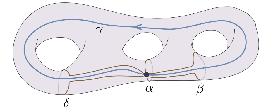
Figure 1. Curves $\alpha,\beta,\gamma,\delta$

Theorem 7.1.

Suppose that $F$ is an essential, connected subsurface of $S$, and that $\alpha,\beta,\delta\in\pi_{1}(F)\subset S$ are represented by based simple loops in F which intersect only at the basepoint, and are freely homotopic to a collection of mutually disjoint and non-parallel, non-separating closed curves in $F$ which do not bound a pair of pants in $F$. If $\rho,\sigma\in\mathcal{H}_{d}(S)$ and $|\operatorname{Tr}(\rho(\eta))|=|\operatorname{Tr}(\sigma(\eta))|$ whenever $\eta\in\pi_{1}(S)$ is represented by a simple closed curve in $F$, then $\rho$ and $\sigma$ are conjugate, in $\mathsf{PGL}_{d}(\mathbb{R})$, on the subgroup $<\alpha,\beta,\delta>$ of $\pi_{1}(S)$.

Proof.

We first show that we can replace $\alpha$, $\beta$ and $\delta$ with based loops in $F$, configured as in Figure 1, which generate the same subgroup of $\pi_{1}(S)$. We then show that if $\alpha$, $\beta$, $\gamma$ and $\delta$ have the form in Figure 1, then $\rho$ and $\sigma$ are conjugate on $\braket{\alpha,\beta,\delta}$.

Lemma 7.2.

Suppose that $F$ is an essential, connected subsurface of $S$, and that $\alpha,\beta,\delta\in\pi_{1}(F)\subset S$ are represented by based simple loops in $F$ which intersect only at the basepoint, and are freely homotopic to a collection of mutually disjoint and non-parallel, non-separating closed curves in $F$ which do not bound a pair of pants in $F$. Then there exist based loops $\hat{\alpha}$, $\hat{\beta}$, $\hat{\gamma}$ and $\hat{\delta}$ in $F$ which intersect only at the basepoint so that $\hat{\alpha}$, $\hat{\beta}$ and $\hat{\delta}$ are freely homotopic to a collection of mutually disjoint and non-parallel, non-separating closed curves, each has geometric intersection one with $\hat{\gamma}$ and

$$\braket{\hat{\alpha},\hat{\beta},\hat{\delta}}=\braket{\alpha,\beta,\delta}.$$

Proof.

We first assume one of the curves, say $\beta$, has the property that the other two curves lie on opposite sides of $\beta$, i.e. there exists a regular neighborhood $N$ of $\beta$, so that $\alpha$ intersects only one component of $N-\beta$ and $\delta$ only intersects the other (see Figure 2).

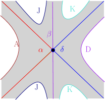
Figure 2. A regular neighborhood of $\alpha\cup\beta\cup\delta$ when $\beta$ locally separates $\alpha$ and $\delta$

Let $F_{1}$ be a regular neighborhood of $T=\alpha\cup\beta\cup\delta.$ Then $F_{1}$ is a four-holed sphere and each component of $F_{1}-T$ is an annulus. We label the boundary components $A$, $D$, $J$ and $K$, where $A$ is parallel to $\alpha$, $D$ is parallel to $\delta$, $J$ is parallel to the based loop $\beta\alpha^{\epsilon_{1}}$ and $K$ is parallel to the based loop $\beta\delta^{\epsilon_{2}}$ for some $\epsilon_{1},\epsilon_{2}\in\{\pm 1\}$.

If $A$ and $D$ lie in the boundary of the same component of $F-F_{1}$, then one may extend an arc in $F-F_{1}$ joining $A$ to $D$ to a closed curve $\hat{\gamma}$ which intersects $T$ only at the basepoint and intersects each of $\alpha$, $\beta$ and $\delta$ with geometric intersection one. In this case, we simply take $\hat{\alpha}=\alpha$, $\hat{\beta}=\beta$ and $\hat{\delta}=\delta$. We assume from now on that $A$ and $D$ do not lie in the same boundary component of $F-F_{1}$.

Since $\alpha$ is non-separating, $A$ must lie in the boundary of a component $G$ of $F-F_{1}$ which also has either $J$ or $K$ in its boundary. If the boundary of $G$ contains $J$ but not $K$, then $\beta$ would separate $F$ which would contradict our assumptions, so the boundary of $G$ must contain $K$. (Recall that by assumption, the boundary of $G$ cannot contain $D$.)

We may then extend an arc in $G$ joining $A$ to $K$ to a closed curve $\hat{\gamma}$ which intersects $T$ only at the basepoint and has geometric intersection one with $\alpha$, $\beta$ and $K$. Moreover, we may choose a based loop $\hat{\delta}$ in the (based) homotopy class of $\beta\delta^{\epsilon_{2}}$ which intersects $\alpha$, $\beta$ and $\hat{\gamma}$ only at the basepoint. In this case, let $\hat{\alpha}=\alpha$ and $\beta=\hat{\beta}$. $A$, $\beta$ and $K$ are simple, disjoint non-separating curves freely homotopic to $\hat{\alpha}$, $\hat{\beta}$ and $\hat{\delta}$. If $K$ is parallel to $A$, then disjoint representative of $\alpha$, $\beta$ and $\delta$ would bound a pair of pants, which is disallowed. Moreover, since $K$ is homotopic to $\beta\delta^{\epsilon_{2}}$ and $\beta$ and $\delta$ are non-parallel simple closed curves, $K$ cannot be parallel to $\beta$ or $\delta$. Since $A$ and $\beta$ are non-parallel, by assumption, $A$, $\beta$ and $K$ are mutually non-parallel as required.

We may now assume that if $\nu\in\{\alpha,\beta,\delta\}$, then there is a regular neighborhood of $\nu$, so that the other two based loops only intersect one component of the regular neighborhood. Let $F_{1}$ be a regular neighborhood of $T$. Again, $F_{1}$ is a four-holed sphere and each component of $F_{1}-T$ is an annulus. We label the components of the boundary of $F_{1}$ by $A$, $B$, $D$ and $E$, where $A$ is parallel to $\alpha$, $B$ is parallel to $\beta$, and $D$ is parallel to $\delta$ (see Figure 3).

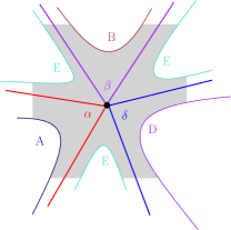
Figure 3. A regular neighborhood of $\alpha\cup\beta\cup\delta$ when no curve locally separates

Since $\alpha$ is non-separating in $F$, there exists a component $G$ of $F-F_{1}$ whose boundary contains $A$ and at least one other component of the boundary of $F_{1}$. If the boundary of $G$ contains $B$, then one may extend an arc in $G$ joining $A$ to $B$ to a curve $\hat{\gamma}$ which intersects $T$ only at the basepoint and has geometric intersection one with $\alpha$ and $\beta$ and geometric intersection zero with $\delta$. Let $\hat{\delta}$ be a simple based loop in $F_{1}$ in the (based) homotopy class of $\alpha\delta^{\epsilon}$ for some $\epsilon\in\{\pm 1\}$ which intersects $\hat{\gamma}$ and $T$ only at the basepoint. Since $\hat{\delta}$ has algebraic intersection $\pm 1$ with $\hat{\gamma}$, it must have geometric intersection one with $\hat{\gamma}$. Let $\hat{\alpha}=\alpha$ and $\hat{\beta}=\beta$, then $\hat{\alpha}$, $\hat{\beta}$ and $\hat{\delta}$ are freely homotopic to the collection $\{A,B,\hat{\delta}\}$ of mutually disjoint, non-separating curves. Notice that $A$ and $B$ are non-parallel by our original assumption, while if $\hat{\delta}$ is parallel to $A$ or $B$, then our original collection of curves would be freely homotopic to the boundary of a pair of pants, contradicting our original assumption. Therefore, $A$, $B$ and $\hat{\delta}$ are non-parallel as required.

If the boundary of $G$, contains $D$, then we may perform the same procedure reversing the roles of $\beta$ and $\delta$. Therefore, we may assume that the boundary of $G$ contains both $A$ and $E$, but not $B$ or $D$. Since $\beta$ is non-separating and $B$ is not in the boundary of $G$, there must be another component $H$ of $F-F_{1}$ which has both $B$ and $D$ in its boundary. We then simply repeat the procedure above to construct a curve $\hat{\gamma}$ which intersects $T$ only at the basepoint which has geometric intersection one with $\beta$ and $\delta$ and geometric intersection zero with $\alpha$. We then let $\hat{\alpha}$ be a simple based loop in $F_{1}$ intersecting $\hat{\gamma}$ only at the basepoint, in the based homotopy class of $\beta\alpha^{\epsilon}$ for some $\epsilon\in\{\pm 1\}$, which has geometric intersection one with $\hat{\gamma}$. Letting $\hat{\beta}=\beta$ and $\hat{\delta}=\delta$, we may complete the proof as in the previous paragraph. ∎

Notice that we may always re-order the curves produced by Lemma 7.2 so that $\hat{\alpha}^{p}\hat{\beta}^{q}\hat{\gamma}\hat{\delta}^{r}$ is represented by a simple non-separating curve in $F$ for all $p,q,r\in\mathbb{Z}$. Moreover, our assumptions imply that $\hat{\alpha}$, $\hat{\beta}$ and $\hat{\delta}$ have non-intersecting axes and that $\hat{\beta}$ and $\hat{\gamma}\hat{\beta}\hat{\gamma}^{-1}$ have non-intersecting axes. Theorem 7.1 will then follow from the following result.

Proposition 7.3.

Suppose that $\alpha,\beta,\gamma,\delta\in\pi_{1}(S)-\{1\}$, $\alpha$, $\beta$ and $\delta$ have non-intersecting axes and that $\beta$ and $\gamma\beta\gamma^{-1}$ have non-intersecting axes. If $\rho,\sigma\in\mathcal{H}_{d}(S)$ and $|\operatorname{Tr}(\rho(\alpha^{p}\beta^{q}\gamma\delta^{r}))|=|\operatorname{Tr}(\sigma(\alpha^{p}\beta^{q}\gamma\delta^{r}))|$ for all $p,q,r\in\mathbb{Z}$, then $\rho$ and $\sigma$ are conjugate, in $\mathsf{PGL}_{d}(\mathbb{R})$, on the subgroup $<\alpha,\beta,\delta>$ of $\pi_{1}(S)$.

Proof.

We may apply Lemma 6.2 to the pairs $(\alpha,\gamma)$, $(\beta,\gamma)$ and $(\delta,\gamma)$ to conclude that $\lambda_{i}(\rho(\eta))=\lambda_{i}(\sigma(\eta))$ for all $i$ and any $\eta\in\{\alpha,\beta,\delta\}$. (Notice, for example, that for the pair $(\alpha,\gamma)$ our assumptions imply that $|\operatorname{Tr}(\rho(\alpha^{n}\gamma))|=|\operatorname{Tr}(\sigma(\alpha^{n}\gamma))|$ for all $n$, so the assumptions of Lemma 6.2 are satisfied.)

Combining the expansions

$$\rho(\alpha)=\sum_{i=1}^{d}\lambda_{i}(\rho(\alpha)){\bf{p}}_{i}(\rho(\alpha))\ \ {\rm and}\ \ \sigma(\alpha)=\sum_{i=1}^{d}\lambda_{i}(\sigma(\alpha)){\bf{p}}_{i}(\sigma(\alpha))$$

with our assumption that $|\operatorname{Tr}(\rho(\alpha^{p}\beta^{q}\gamma\delta^{r}))|=|\operatorname{Tr}(\sigma(\alpha^{p}\beta^{q}\gamma\delta^{r}))|$ for all $p,q,r\in\mathbb{Z}$, we see that

$$\sum_{i=1}^{d}\lambda_{i}^{p}(\rho(\alpha))\operatorname{Tr}\left({\bf{p}}_{i}(\rho(\alpha))\rho(\beta^{q}\gamma\delta^{r})\right)=\pm\sum_{i=1}^{d}\lambda_{i}^{p}(\sigma(\alpha))\operatorname{Tr}\left({\bf{p}}_{i}(\sigma(\alpha))\sigma(\beta^{q}\gamma\delta^{r})\right)$$

for all $p,q,r\in\mathbb{N}$. Since $\rho(\alpha)$ and $\sigma(\alpha)$ are purely loxodromic and $\lambda_{i}(\rho(\alpha))=\lambda_{i}(\sigma(\alpha))$ for all $i$, we may fix $q$ and $r$, let $p$ tend to $+\infty$ and consider terms of the same order to conclude that

$$\operatorname{Tr}\left({\bf{p}}_{i}(\rho(\alpha))\rho(\beta^{q}\gamma\delta^{r})\right)=\pm\operatorname{Tr}\left({\bf{p}}_{i}(\sigma(\alpha))\sigma(\beta^{q}\gamma\delta^{r})\right)$$ (2)

for all $i\in\{1,\ldots,d\}$ and all $q,r\in\mathbb{N}$. Similarly, we expand Equation (2) to see that, for all $i$,

$$\sum_{j=1}^{d}\lambda_{j}^{q}(\rho(\beta))\operatorname{Tr}\left({\bf{p}}_{i}(\rho(\alpha)){\bf{p}}_{j}(\rho(\beta))\rho(\gamma\delta^{r})\right)=\pm\sum_{j=1}^{d}\lambda_{j}^{q}(\sigma(\beta))\operatorname{Tr}\left({\bf{p}}_{i}(\sigma(\alpha)){\bf{p}}_{j}(\sigma(\beta))\sigma(\gamma\delta^{r})\right)$$

and consider terms of the same order as $q\to+\infty$ to conclude that

$$\operatorname{Tr}\left({\bf{p}}_{i}(\rho(\alpha)){\bf{p}}_{j}(\rho(\beta))\rho(\gamma\delta^{r})\right)=\pm\operatorname{Tr}\left({\bf{p}}_{i}(\sigma(\alpha)){\bf{p}}_{i}(\sigma(\beta))\sigma(\gamma\delta^{r})\right)$$

for all $i,j\in\{1,\ldots,d\}$ and $r\in\mathbb{N}$. Expanding this last equation and letting $r$ tend to $+\infty$, we finally conclude that

$$\operatorname{Tr}({\bf{p}}_{i}(\rho(\alpha)){\bf{p}}_{j}(\rho(\beta))\rho(\gamma){\bf{p}}_{k}(\rho(\delta)))=\pm\operatorname{Tr}({\bf{p}}_{i}(\sigma(\alpha)){\bf{p}}_{j}(\sigma(\beta))\sigma(\gamma){\bf{p}}_{k}(\sigma(\delta)))$$

for all $i,j,k\in\{1,\ldots,d\}$, i.e.

$${\bf T}_{i,j,0,k}(\alpha,\beta,\gamma,\delta)(\rho)=\pm{\bf T}_{i,j,0,k}(\alpha,\beta,\gamma,\delta)(\sigma)$$ (3)

for all $i,j,k\in\{1,\ldots,d\}.$

We similarly expand the equation

$$\operatorname{Tr}(\rho(\beta^{q}\gamma\delta^{r}))=\pm\operatorname{Tr}(\sigma(\beta^{q}\gamma\delta^{r}))$$

to see that

$${\bf T}_{j,0,k}(\beta,\gamma,\delta)(\rho)=\pm{\bf T}_{j,0,k}(\beta,\gamma,\delta)(\sigma)$$ (4)

for all $j$ and $k$.

Recall, from part (4) of Proposition 4.3, that

$${\bf T}_{i,j,0,k}(\alpha,\beta,\gamma,\delta)(\rho)={\bf T}_{j,0,k}(\beta,\gamma,\delta)(\rho)\left(\frac{{\bf T}_{i,j,k}(\alpha,\beta,\delta)(\rho)}{{\bf T}_{j,k}(\beta,\delta)(\rho)}\right)\neq 0$$

for all $\rho\in{\mathcal{H}}_{d}(S)$ and $i,j,k\in\{1,\ldots,d\}$, so we may conclude from Equations (3) and (4) that

$$\frac{{\bf T}_{i,j,k}(\alpha,\beta,\delta)(\rho)}{{\bf T}_{j,k}(\beta,\delta)(\rho)}=\pm\frac{{\bf T}_{i,j,k}(\alpha,\beta,\delta)(\sigma)}{{\bf T}_{j,k}(\beta,\delta)(\sigma)}$$

for all $i,j,k\in\{1,\ldots,d\}$.

We may join $\rho$ to $\sigma$ by a path $\{\rho_{t}\}$ of Hitchin representations. So, since $\frac{{\bf T}_{i,j,k}(\alpha,\beta,\delta)(\rho_{t})}{{\bf T}_{j,k}(\beta,\delta)(\rho_{t})}$ is non-zero for all $t$, again by Proposition 4.3, and varies continuously, it follows that

$$\frac{{\bf T}_{i,j,k}(\alpha,\beta,\delta)(\rho)}{{\bf T}_{j,k}(\beta,\delta)(\rho)}=\frac{{\bf T}_{i,j,k}(\alpha,\beta,\delta)(\sigma)}{{\bf T}_{j,k}(\beta,\delta)(\sigma)}$$

for all $i,j,k\in\{1,\ldots,d\}$. Therefore, since we have already seen that $\lambda_{i}(\rho(\eta))=\lambda_{i}(\sigma(\eta))$ for all $i$ if $\eta\in\{\alpha,\beta,\gamma\}$, Theorem 4.4 implies that $\rho$ and $\sigma$ are conjugate, in $\mathsf{PGL}_{d}(\mathbb{R})$, on the subgroup $<\alpha,\beta,\delta>$ of $\pi_{1}(S)$. ∎

∎

We are now ready to establish that the restriction of the marked trace spectrum to the simple non-separating curves determines a Hitchin representation.

Theorem 7.4.

Let $S$ be a closed orientable surface of genus $g\geqslant 3$. If $\rho\in{\mathcal{H}}_{d_{1}}(S)$, $\sigma\in\mathcal{H}_{d_{2}}(S)$ and $|\operatorname{Tr}(\rho(\alpha))|=|\operatorname{Tr}(\sigma(\alpha))|$ whenever $\alpha\in\pi_{1}(S)$ is represented by a simple non-separating curve, then $d_{1}=d_{2}$ and $\rho=\sigma$.

Proof.

Notice that Theorem 6.1 immediately implies that $d_{1}=d_{2}$, so we may assume that $d=d_{1}=d_{2}$. Consider the standard generating set

$$\mathcal{S}=\{\alpha_{1},\beta_{1},\ldots,\alpha_{g},\beta_{g}\}$$

for $\pi_{1}(S)$ so that $\prod_{i=1}^{g}[\alpha_{i},\beta_{i}]=1$, each generator is represented by a based loop, and any two such based loops intersect only at the basepoint.

Notice that the generators are freely homotopic to simple, non-separating closed curves so that the representative of $\alpha_{i}$ is disjoint from the representative of every other generator except $\beta_{i}$ and that the representative of $\beta_{i}$ is disjoint from the representative of every other generator except $\alpha_{i}$. Moreover, no three of the representatives which are disjoint bound a pair of pants. Therefore, Theorem 7.1 implies that we may assume that $\rho$ and $\sigma$ agree on $<\alpha_{1},\alpha_{2},\alpha_{3}>$.

If $\eta\in\mathcal{S}-\{\alpha_{1},\alpha_{2},\beta_{1},\beta_{2}\}$, then Theorem 7.1 implies that there exists $C\in\mathsf{PGL}_{d}(\mathbb{R})$ so that $\rho$ and $C\sigma C^{-1}$ agree on $<\alpha_{1},\alpha_{2},\eta>$. Since $\rho$ and $\sigma$ agree on $\alpha_{1}$ and $\alpha_{2}$, the following lemma, which we memorialize for repeated use later in the paper, assures that $C=I$, so $\rho(\eta)=\sigma(\eta)$.

Lemma 7.5.

Suppose that $S$ is a closed surface of genus at least two, $\rho:\pi_{1}(S)\to\mathsf{PSL}_{d}(\mathbb{R})$ and $\sigma:\pi_{1}(S)\to\mathsf{PSL}_{d}(\mathbb{R})$ are Hitchin representations, and there exists a subgroup $H$ of $\pi_{1}(S)$ and $C\in\mathsf{PSL}_{d}(\mathbb{R})$ so that $\rho|_{H}=C\sigma|_{H}C^{-1}$. If there exists $\nu_{1},\nu_{2}\in H$ with non-intersecting axes, so that $\rho(\nu_{1})=\sigma(\nu_{1})$ and $\rho(\nu_{2})=\sigma(\nu_{2})$, then $C=I$, so $\rho|_{H}=\sigma|_{H}$.

Proof.

Since $\rho$ and $\sigma$ agree on $\nu_{1}$ and $\nu_{2}$, $C$ must commute with $\rho(\nu_{1})$ and $\rho(\nu_{2})$. Thus $C$ is diagonalizable over $\mathbb{R}$ with respect to both $\{e_{i}(\rho(\nu_{1}))\}$ and $\{e_{i}(\rho(\nu_{2})\}$. If $C\neq I$, then $\mathbb{R}^{d}$ admits a non-trivial decomposition into eigenspaces of $C$ with distinct eigenvalues. Any such eigenspace $W$ is spanned by a sub-collection of $\{e_{i}(\rho(\nu_{1}))\}$ and by a sub-collection of $\{e_{j}(\rho(\nu_{2}))\}$. In particular, some $e_{i}(\rho(\nu_{1}))$ is in the subspace spanned by a subcollection of $\{e_{j}(\rho(\nu_{2}))\}$. Since $\nu_{1}$ and $\nu_{2}$ have non-intersecting axes, this contradicts Corollary 4.1. Therefore, $C=I$. ∎

In order to prove that $\rho(\beta_{1})=\sigma(\beta_{1})$, we similarly apply Theorem 7.1 and Lemma 7.5 to the elements $\alpha_{2}$, $\alpha_{3}$ and $\beta_{1}$, while to prove that $\rho(\beta_{2})=\sigma(\beta_{2})$ we consider the elements $\alpha_{1}$, $\alpha_{3}$ and $\beta_{2}$. Since we have established that $\rho$ and $\sigma$ agree on every element in the generating set $\mathcal{S}$, we conclude that $\rho=\sigma$. ∎

Marked simple length rigidity, Theorem 1.1, is an immediate consequence of Theorems 7.4 and 6.1.

We may further use the Noetherian property of polynomial rings to prove the final statement in Theorem 1.2, which asserts that Hitchin representations of the same dimension are determined by the traces of a finite set of simple non-separating curves.

Proof of Theorem 1.2.

We consider the affine algebraic variety

$$V(S)=\operatorname{Hom}(\pi_{1}(S),\mathsf{SL}_{d}(\mathbb{R}))\times\operatorname{Hom}(\pi_{1}(S),\mathsf{SL}_{d}(\mathbb{R})).$$

Let $\{\gamma_{i}\}_{i=1}^{\infty}\subset\pi_{1}(S)$ be an ordering of the collection of (conjugacy classes of) elements of $\pi_{1}(S)$ which are represented by simple, non-separating curves, and define, for each $n$,

$$V_{n}(S)=\left\{(\rho,\sigma)\in V(S)\ |\ \operatorname{Tr}(\rho(\gamma_{i}))=\operatorname{Tr}(\sigma(\gamma_{i}))\ {\rm if}\ \ i\leqslant n\right\}$$

and let

$$V_{\infty}=\bigcap_{n=1}^{\infty}V_{n}.$$

Then each $V_{n}(S)$ is a subvariety of $V(S)$ and by the Noetherian property of polynomial rings, there exists $N$ so that $V_{N}=V_{\infty}$. We define $\mathcal{L}_{d}(S)=\{\gamma_{i}\}_{i=1}^{N}$.

There exists a component ${\widetilde{\mathcal{H}}}_{d}(S)$ of $\operatorname{Hom}(\pi_{1}(S),\mathsf{SL}_{d}(\mathbb{R}))$ consisting of lifts of Hitchin representations so that ${\mathcal{H}}_{d}(S)$ is identified with the quotient of ${\widetilde{\mathcal{H}}}_{d}(S)$ by $\mathsf{SL}_{d}(\mathbb{R})$, see Hitchin [20]. Since traces of elements in images of (lifts of) Hitchin representations are non-zero, for all $\gamma\in\pi_{1}(S)$, $\operatorname{Tr}(\nu(\gamma))$ is either positive for all $\nu\in{\widetilde{\mathcal{H}}}_{d}(S)$ or negative for all $\nu\in{\widetilde{\mathcal{H}}}_{d}(S)$, for all $\gamma\in\pi_{1}(S)$. Therefore, if the marked trace spectra of $\rho,\sigma\in\mathcal{H}_{d}(S)$ agree on $\mathcal{L}_{d}(S)$, they admit lifts $\tilde{\rho}$ and $\tilde{\sigma}$ in ${\widetilde{\mathcal{H}}}_{d}(S)$ so that $(\tilde{\rho},\tilde{\sigma})\in V_{N}$. Since $V_{N}=V_{\infty}$, the marked trace spectra of $\rho$ and $\sigma$ agree on all simple, non-separating curves. Therefore, by Theorem 7.4, $\rho=\sigma\in{\mathcal{H}}_{d}(S)$. ∎

Remark: The set $\mathcal{L}_{d}(S)$ contains at least $\dim({\mathcal{H}}_{d}(S))=-\chi(S)(d^{2}-1)$ curves, but our methods do not provide any upper bound on the size of $\mathcal{L}_{d}(S)$.

8. Isometries of intersection

In this section, we investigate isometries of the intersection function which is used to construct the pressure metric on the Hitchin component. Our main tool will be Bonahon’s theory of geodesic currents and his reinterpretation of Thurston’s compactification of Teichmüller space in this language, see Bonahon [3].

8.1. Intersection and the pressure metric

Given $\rho\in{\mathcal{H}}_{d}(S)$, let

$$R_{T}(\rho)=\left\{[\gamma]\ \in[\pi_{1}(S)]\ |\ L_{\gamma}(\rho)\leqslant T\right\}$$

be the set of conjugacy classes of elements of $\pi_{1}(S)$ whose images have length at most $T$. One may then define the entropy

$$h(\rho)=\lim_{T\rightarrow\infty}\frac{\log(\#R_{T}(\rho))}{T}.$$

Given $\rho,\sigma\in{\mathcal{H}}_{d}(S)$, their intersection is given by

$${\bf I}(\rho,\sigma)=\lim_{T\rightarrow\infty}\frac{1}{\#R_{T}(\rho)}\sum_{[\gamma]\in R_{T}(\rho)}\frac{L_{\gamma}(\sigma)}{L_{\gamma}(\rho)}.$$

and their renormalized intersection is given by

$${\bf J}(\rho,\sigma)=\frac{h(\sigma)}{h(\rho)}I(\rho,\sigma).$$

One may show that all the quantities above give rise to analytic functions.

Theorem 8.1.

(Bridgeman–Canary–Labourie–Sambarino [7, Thm. 1.3]) If $S$ is a closed surface of genus greater than 1, the entropy $h$, the intersection ${\bf I}$, and renormalized intersection ${\bf J}$ are analytic functions on ${\mathcal{H}}_{d}(S)$, ${\mathcal{H}}_{d}(S)\times{\mathcal{H}}_{d}(S)$ and ${\mathcal{H}}_{d}(S)\times{\mathcal{H}}_{d}(S)$ respectively.

Let ${\bf J}_{\rho}:{\mathcal{H}}_{d}(S)\to\mathbb{R}$ be defined by ${\bf J}_{\rho}(\sigma)={\bf J}(\rho,\sigma)$. The analytic function ${\bf J}_{\rho}$ has a minimum at $\rho$ (see [7, Thm. 1.1]) and hence its Hessian gives rise to an non-negative quadratic form on $T_{\rho}({\mathcal{H}}_{d}(S))$, called the pressure metric. Bridgeman, Canary, Labourie and Sambarino proved that the resulting quadratic form is positive definite. A result of Wolpert [35] implies that the restriction of the pressure metric to the Fuchsian locus is a multiple of the classical Weil-Petersson metric. (See [8] for a survey of this theory.)

Theorem 8.2.

(Bridgeman–Canary–Labourie–Sambarino [7, Cor. 1.6]) If $S$ is a closed surface of genus greater than 1, the pressure metric is a mapping class group invariant, analytic, Riemannian metric on ${\mathcal{H}}_{d}(S)$ whose restriction to the Fuchsian locus is a multiple of the Weil-Petersson metric.

Recall that a diffeomorphism $f:{\mathcal{H}}_{d}(S)\to{\mathcal{H}}_{d}(S)$ is said to be an isometry of intersection if ${\bf I}(f(\rho),f(\sigma))={\bf I}(\rho,\sigma)$ for all $\rho,\sigma\in{\mathcal{H}}_{d}(S)$. Let ${\rm Isom}_{\bf I}({\mathcal{H}}_{d}(S))$ denote the group of isometries of ${\bf I}$. Notice that, by construction, the extended mapping class group ${\rm Mod}(S)$ is a subgroup of ${\rm Isom}_{\bf I}({\mathcal{H}}_{d}(S))$. (The extended mapping class group ${\rm Mod}(S)$ can be identified with the group ${\rm Out}(\pi_{1}(S))$ of outer automorphisms of $\pi_{1}(S)$ and acts naturally on ${\mathcal{H}}_{d}(S)$ by pre-composition.)

The entire discussion of intersection, renormalized intersection and the pressure metric restricts to $\mathsf{H}(S,\mathsf{G})$ when $\mathsf{G}$ is $\mathsf{PSp}(2d,\mathbb{R}),$ $\mathsf{PSO}(d,d+1)$, or $\mathsf{G}_{2,0}$.

8.2. Basic properties

We first show that isometries of intersection preserve entropy and hence preserve renormalized intersection, so are isometries of the pressure metric.

Proposition 8.3.

If $S$ is a closed orientable surface of genus greater than 1, $\mathsf{G}$ is $\mathsf{PSL}_{d}(\mathbb{R})$, $\mathsf{PSp}(2d,\mathbb{R}),$ $\mathsf{PSO}(d,d+1)$, or $\mathsf{G}_{2,0}$ and $f:\mathcal{H}(S,\mathsf{G})\to\mathcal{H}(S,\mathsf{G})$ is an isometry of intersection ${\bf I}$, then $h(\rho)=h(f(\rho))$ for all $\rho\in\mathcal{H}(S,\mathsf{G})$. Therefore, ${\bf J}(f(\rho),f(\sigma))={\bf J}(\rho,\sigma)$ for all $\rho,\sigma\in\mathcal{H}(S,\mathsf{G})$, and $f$ is an isometry of $\mathcal{H}(S,\mathsf{G})$ with respect to the pressure metric.

Proof.

Suppose that $\rho\in{\mathcal{H}}(S,\mathsf{G})$, $v\in\mathsf{T}_{\rho}({\mathcal{H}}(S,\mathsf{G}))$ and $v=\frac{d}{dt}\rho_{t}=\mathrel{\mathop{\rho}\limits^{\vbox to0.0pt{\kern-2.0pt\hbox{$\scriptstyle\bullet$}\vss}}}\!\!_{0}$ for a smooth path $\{\rho_{t}\}_{t\in(-1,1)}$ in ${\mathcal{H}}_{d}(S)$. Then,

$${\bf I}_{\rho}(\rho_{t})={\bf I}(\rho,\rho_{t})={\bf I}(f(\rho),f(\rho(t))={\bf I}_{f(\rho)}(f(\rho_{t})),$$

so

$${\rm D}{\bf I}_{\rho}(v)={\rm D}{\bf I}_{f(\rho)}({\rm D}f_{\rho}(v)).$$

Since ${\bf J}_{\rho}$ has a minimum at $\rho$, ${\rm D}{\bf J}_{\rho}(v)=0$, so

$${\rm D}{\bf J}_{\rho}(v)=\frac{{\rm D}h_{\rho}(v)}{h(\rho)}{\bf I}_{\rho}(\rho)+\frac{h(\rho)}{h(\rho)}{\rm D}{\bf I}_{\rho}(v)=\frac{{\rm D}h_{\rho}(v)}{h(\rho)}+{\rm D}{\bf I}_{\rho}(v)=0$$

which implies that

$${\rm D}{\bf I}_{\rho}(v)=-\frac{{\rm D}h_{\rho}(v)}{h(\rho)}=-{\rm D}(\log{h})(v).$$

Thus, for all $v\in T_{\rho}({\mathcal{H}}(S,\mathsf{G}))$

$${\rm D}(\log{h})(v)={\rm D}(\log(h\circ f))(v),$$

so $(h\circ f)/h$ is constant, since ${\mathcal{H}}(S,\mathsf{G})$ is a connected manifold. However, since $h$ is a bounded positive function, it must be the case that $h\circ f=h$.

It follows, by the definition of renormalized intersection, that $f$ preserves renormalized intersection. Since the pressure metric is obtained by considering the Hessian of renormalized intersection, $f$ is also an isometry of $\mathcal{H}(S,\mathsf{G})$ with respect to the pressure metric. ∎

Potrie and Sambarino [31] proved that the entropy function achieves its maximum exactly on the Fuchsian locus, so we have the following immediate corollary.

Corollary 8.4.

If $S$ is a closed orientable surface of genus greater than 1, $\mathsf{G}$ is $\mathsf{PSL}_{d}(\mathbb{R})$, $\mathsf{PSp}(2d,\mathbb{R}),$ $\mathsf{PSO}(d,d+1)$, or $\mathsf{G}_{2,0}$ and $f:\mathcal{H}(S,\mathsf{G})\to\mathcal{H}(S,\mathsf{G})$ is an isometry of intersection ${\bf I}$, then $f$ preserves the Fuchsian locus.

8.3. Geodesic currents

We identify $S$ with a fixed hyperbolic surface ${\bf H}^{2}/\Gamma$, which in turn identifies $\pi_{1}(S)$ with $\Gamma$ and $\partial_{\infty}\pi_{1}(S)$ with $\partial_{\infty}{\bf H}^{2}$. One can identify the space $G({\bf H}^{2})$ of unoriented geodesics in ${\mathbb{H}}^{2}$ with $(\partial_{\infty}{\bf H}^{2}\times\partial_{\infty}{\bf H}^{2}-\Delta)/\mathbb{Z}_{2}$, where $\Delta$ is the diagonal in $\partial_{\infty}{\bf H}^{2}\times\partial_{\infty}{\bf H}^{2}$ and $\mathbb{Z}_{2}$ acts by interchanging coordinates. A geodesic current on $S$ is a $\Gamma$-invariant Borel measure on $G({\bf H}^{2})$ and ${\mathcal{C}}(S)$ is the space of geodesic currents on $S$, endowed with the weak^∗ topology.

If $\alpha$ is a closed geodesic on $S$, one obtains a geodesic current $\delta_{\alpha}$ by taking the sum of the Dirac measures on the pre-images of $\alpha$. The set of currents which are scalar multiples of closed geodesics is dense in $\mathcal{C}(S)$, see Bonahon [3, Proposition 2]. If $\rho\in\mathcal{T}(S)=\mathcal{H}_{2}(S)$ has associated limit map $\xi_{\rho}:\partial\pi_{1}(S)\to\partial\mathbb{H}_{2}$, one defines the Liouville measure of $\rho$ by

$$m_{\rho}([a,b]\times[c,d])=\left|\log\frac{\big{(}\xi_{\rho}(a)-\xi_{\rho}(c)\big{)}\big{(}\xi_{\rho}(b)-\xi_{\rho}(d)\big{)}}{\big{(}\xi_{\rho}(a)-\xi_{\rho}(d)\big{)}\big{(}\xi_{\rho}(b)-\xi_{\rho}(c)\big{)}}\right|.$$

Theorem 8.5.

(Bonahon [3, Propositions 3, 14, 15]) Let $S$ be a closed oriented surface of genus $g\geqslant 2$ and $\rho\in\mathcal{T}(S)=\mathcal{H}_{2}(S)$. Then there exist continuous functions $\ell_{\rho}:{\mathcal{C}}(S)\rightarrow\mathbb{R}$ and $i:{\mathcal{C}}(S)\times{\mathcal{C}}(S)\rightarrow\mathbb{R}$ which are linear on rays such that if $\alpha$ and $\beta$ are closed geodesics, then

$$i(m_{\rho},\delta_{\alpha})=\ell_{\rho}(\alpha),\quad i(m_{\rho},m_{\rho})=\pi^{2}|\chi(S)|,$$

and $i(\alpha,\beta)$ is the geometric intersection between $\alpha$ and $\beta$.

Moreover, Bonahon defines an embedding

$$Q:{\mathcal{T}}(S)\rightarrow{\mathcal{P}C}(S)$$

of Teichmüller space into the space of projective classes of geodesic currents given by $Q(\rho)=[m_{\rho}]$. Bonahon shows that the closure of $Q(\mathcal{T}(S))$ is homeomorphic to a closed ball of dimension $6g-6$, and the boundary of $Q(\mathcal{T}(S))$ is the space $\mathcal{PML}(S)$ of projective classes of measured laminations. (Recall that a measured lamination may be defined to be a geodesic current of self-intersection 0.) In particular, the geodesic current associated to any simple closed curve lies in the boundary of $Q(\mathcal{T}(S))$. Moreover, Bonahon [3, Theorem 18] shows that this compactification of Teichmüller space agrees with Thurston’s compactification.

8.4. Length functions for Hitchin representations

If $\rho\in{\mathcal{H}}_{d}(S)$, then there is a Hölder function $f_{\rho}:T^{1}S\rightarrow\mathbb{R}_{+}$ such that if $\alpha$ is a closed oriented geodesic on $S={\bf H}^{2}/\Gamma$, then

$$\int_{\alpha}f_{\rho}\ dt=L_{\alpha}(\rho)$$

where $dt$ is the Lebesgue measure along $\alpha\subset T^{1}(S)$, see [7, Prop. 4.1] or Sambarino [33, Sec. 5]. Given $\mu\in\mathcal{C}(S)$, one may define a $\Gamma$-invariant measure $\tilde{\mu}$ on $\mathsf{T}^{1}{\bf H}^{2}$ which has the local form $\mu\times dt$ where $dt$ is Lebesgue measure along the flow lines of $\mathsf{T}^{1}{\bf H}^{2}$ (which are oriented geodesics in ${\bf H}^{2}$), so $\tilde{\mu}$ descends to a measure $\hat{\mu}$ on $T^{1}(S)$. One may then define a length function $\ell_{\rho}:{\mathcal{C}}(S)\rightarrow\mathbb{R}$ by letting

$$\ell_{\rho}(\mu)=\int_{T^{1}(S)}f_{\rho}\ d\hat{\mu}.$$

Notice that if $\alpha$ is a simple closed geodesic on $S$, then

$$\ell_{\rho}(\delta_{\alpha})=L^{H}_{\alpha}(\rho)=L_{\alpha}(\rho)+L_{\alpha^{-1}}(\rho)$$

since $\hat{\delta}_{\alpha}$ is Dirac measure support on the closed orbits of geodesics associated to $\alpha$ and $\alpha^{-1}$. Moreover, by the definition of the weak^∗ topology, $\ell_{\rho}$ is clearly continuous, since $T^{1}S$ is compact.

Recall that (see Bowen [4] or Margulis [28]) if $\sigma\in\mathcal{T}(S)=\mathcal{H}_{2}(S)$ then the Liouville current satisfies

$$\frac{m_{\sigma}}{\ell_{\sigma}(m_{\sigma})}=\lim_{T\rightarrow\infty}\frac{1}{\#R_{T}(\sigma)}\sum_{R_{T}(\sigma)}\frac{\delta_{\alpha}}{\ell_{\sigma}(\delta_{\alpha})}=\lim_{T\rightarrow\infty}\frac{1}{\#R_{T}(\sigma)}\sum_{R_{T}(\sigma)}\frac{\delta_{\alpha}}{2L_{\alpha}(\sigma)}.$$

Since $\tau_{d}$ multiplies the logarithm of the spectral radius by $d-1$, if $\rho\in{\mathcal{H}}_{d}(S)$, then

$$\frac{\ell_{\rho}(m_{\sigma})}{\ell_{\sigma}(m_{\sigma})} = \lim_{T\rightarrow\infty}\frac{1}{\#R_{T}(\sigma)}\sum_{R_{T}(\sigma)}\frac{L^{H}_{\alpha}(\rho)}{2L_{\alpha}(\sigma)}$$

$$= \left(d-1\right)\ \lim_{T\rightarrow\infty}\frac{1}{\#R_{(d-1)T}(\tau_{d}\circ\sigma)}\sum_{R_{(d-1)T}(\tau_{d}\circ\sigma)}\frac{L_{\alpha}(\rho)}{L_{\alpha}(\tau_{d}\circ\sigma)}$$

$$= \left(d-1\right)\ {\bf I}(\tau_{d}\circ\sigma,\rho).$$

Here we use the fact that, since $\sigma\in\mathcal{T}(S)$, $L_{\alpha}(\sigma)=L_{\alpha^{-1}}(\sigma)$, so

$$\frac{L^{H}_{\alpha}(\rho)}{2L_{\alpha}(\sigma)}+\frac{L^{H}_{\alpha^{-1}}(\rho)}{2L_{\alpha^{-1}}(\sigma)}=\frac{L_{\alpha}(\rho)}{L_{\alpha}(\sigma)}+\frac{L_{\alpha^{-1}}(\rho)}{L_{\alpha^{-1}}(\sigma)}$$

for all $\alpha\in\pi_{1}(S)$.

8.5. Isometries of intersection and the simple Hilbert length spectrum

We next observe that any isometry of intersection preserves the simple marked Hilbert length spectrum.

Proposition 8.6.

If $S$ is a closed surface of genus $g\geqslant 2$, $\mathsf{G}=\mathsf{PSL}_{d}(\mathbb{R})$, $\mathsf{PSp}(2d,\mathbb{R}),$ $\mathsf{PSO}(d,d+1)$, or $\mathsf{G}_{2,0}$ and $f:\mathcal{H}(S,\mathsf{G})\to\mathcal{H}(S,\mathsf{G})$ is an isometry of intersection, then there exists an element $\phi$ of the extended mapping class group so that if $\rho\in\mathcal{H}(S,\mathsf{G})$, then $\rho$ and $f\circ\phi(\rho)$ have the same simple marked Hilbert length spectrum.

Proof.

Recall, from Corollary 8.4, that $f$ preserves the Fuchsian locus. Since any isometry of $\mathcal{T}(S)$ with the Weil-Petersson metric agrees with an element of the extended mapping class group, by a result of Masur-Wolf [29], and the restriction of the pressure metric to the Fuchsian locus is a multiple of the Weil-Petersson metric, the restriction of $f$ to the Fuchsian locus agrees with the action of an element $\phi$ of the extended mapping class group. We can thus consider $\hat{f}=f\circ\phi^{-1}$, which is an isometry of the intersection function that fixes the Fuchsian locus.

If $\alpha\in\pi_{1}(S)$ is represented by a simple curve, we may choose a sequence $\{\sigma_{n}\}$ in $\mathcal{T}(S)$ such that $\{Q(\sigma_{n})\}$ converges to $[\delta_{\alpha}]\in\mathcal{PC}(S)$, so there exists a sequence $\{c_{n}\}$ of real numbers so that $\lim c_{n}=+\infty$ and

$$\lim\frac{m_{\sigma_{n}}}{c_{n}}=\delta_{\alpha}.$$

Therefore, if $\rho\in\mathcal{H}(S,\mathsf{G})\subset{\mathcal{H}}_{d}(S)$, then

$$L^{H}_{\alpha}(\rho)=\ell_{\rho}(\delta_{\alpha})=\lim\ell_{\rho}\left(\frac{m_{\sigma_{n}}}{c_{n}}\right)=\lim\left(\frac{(d-1)\ell_{\sigma_{n}}(m_{\sigma_{n}})}{c_{n}}{\bf I}(\tau_{d}\circ\sigma_{n},\rho)\right).$$

By Theorem 8.5, as $\sigma_{n}\in\mathcal{T}(S)$, then $\ell_{\sigma_{n}}(m_{\sigma_{n}})=i(m_{\sigma_{n}},m_{\sigma_{n}})=\pi^{2}|\chi(S)|$. If $\rho\in\mathcal{H}(S,\mathsf{G})$ and $\alpha\in\pi_{1}(S)$, then since ${\bf I}(\tau_{d}\circ\sigma_{n},\rho)={\bf I}(\tau_{d}\circ\sigma_{n},\hat{f}(\rho))$ for all $n$, $L^{H}_{\alpha}(\rho)=L^{H}_{\alpha}(\hat{f}(\rho))$. Therefore, $\rho$ and $\hat{f}(\rho)$ have the same simple marked Hilbert length spectrum. ∎

Recall that if $\rho$ lies in $\mathcal{H}(S,\mathsf{G})$ and $\mathsf{G}$ is $\mathsf{PSp}(2d,\mathbb{R})$, $\mathsf{PSO}(d,d+1)$ or $\mathsf{G}_{2,0}$, then $L^{H}_{\alpha}(\rho)=2L_{\alpha}(\rho)$ for all $\alpha\in\pi_{1}(S)$. Therefore, we may combine Theorem 1.1 and Proposition 8.6 to obtain:

Corollary 8.7.

If $S$ is a closed surface of genus $g\geqslant 3$, then any isometry of the intersection ${\bf I}$ on $\mathcal{H}(S,\mathsf{PSp}(2d,\mathbb{R}))$, $\mathcal{H}(S,\mathsf{PSO}(d,d+1))$, or $\mathcal{H}(S,\mathsf{G}_{2,0})$ agrees with an element of the extended mapping class group.

Notice that Corollary 8.7 is a generalization of Theorem 1.3 which was stated in the introduction.

9. Hilbert Length Rigidity

Proposition 8.6 suggests the following potential generalization of our main simple length rigidity result.

Conjecture: If $\rho,\sigma\in{\mathcal{H}}_{d}(S)$ have the same marked simple Hilbert length spectrum then they either agree or differ by the contragredient involution.

We establish this conjecture when $d=3$.

Theorem 9.1.

If $S$ is a closed orientable surface of genus greater than 2, $\rho,\sigma\in{\mathcal{H}}_{3}(S)$ and $L^{H}_{\alpha}(\rho)=L^{H}_{\alpha}(\sigma)$ for any $\alpha\in\pi_{1}(S)$ which is represented by a simple non-separating curve, then $\rho=\sigma$ or $\rho=\sigma^{*}$.

The classification of the isometries of intersection on $\mathcal{H}_{3}(S)$, Theorem 1.4, is an immediate consequence of Theorem 9.1 and Proposition 8.6.

Proof.

Notice that $\mathsf{PSL}_{3}(\mathbb{R})=\mathsf{SL}_{3}(\mathbb{R})$ and that if $\gamma\in\pi_{1}(S)$, then all the eigenvalues of $\rho(\gamma)$ are positive, since eigenvalues vary continuously over $\mathcal{H}_{3}(S)$ and are positive on the Fuchsian locus. In particular, if $L^{H}_{\alpha}(\rho)=L^{H}_{\alpha}(\sigma)$, then

$$\frac{\lambda_{1}(\rho(\alpha))}{\lambda_{3}(\rho(\alpha))}=\frac{\lambda_{1}(\sigma(\alpha))}{\lambda_{3}(\sigma(\alpha))}>1.$$

We first show that for individual elements the traces and eigenvalues either agree or are consistent with the contragredient involution.

Lemma 9.2.

If $\alpha$ and $\beta$ are represented by simple, non-separating based loops on $S$ which intersect only at the basepoint and have geometric intersection one, and $L^{H}_{\alpha^{n}\beta}(\rho)=L^{H}_{\alpha^{n}\beta}(\sigma)$ for all $n$, then either

1. $\lambda_{i}(\rho(\alpha))=\lambda_{i}(\sigma(\alpha))$ for all $i$, so $\operatorname{Tr}(\rho(\alpha))=\operatorname{Tr}(\sigma(\alpha))$, or

2. $\lambda_{i}(\rho(\alpha))=\lambda_{i}(\sigma(\alpha^{-1}))=\lambda_{i}(\sigma^{*}(\alpha))$ for all $i$, so $\operatorname{Tr}(\rho(\alpha))=\operatorname{Tr}(\sigma^{*}(\alpha))$.

Proof.

As in the proof of Lemma 6.3, let $A=\rho(\alpha)$, $B=\rho(\beta)$ and $A^{n}B=\rho(\alpha^{n}\beta)$ and $\lambda_{i}(n)=\lambda_{i}(A^{n}B)$. Similarly, let $\hat{A}=\sigma(\alpha)$, $\hat{B}=\sigma(\beta)$ and $\hat{A}^{n}\hat{B}=\sigma(\alpha^{n}\beta)$ and let $\hat{\lambda}_{i}(n)=\lambda_{i}(\hat{A}^{n}\hat{B})$. If $(b^{i}_{j})$ is the matrix of $B$ with respect to the basis $\{e_{i}(A)\}$, then, $b^{1}_{1}$, $b^{1}_{2}$, and $b^{2}_{1}$ are all non-zero by Lemma 6.4, so Lemma 5.1 implies that

$$\frac{\lambda_{1}(n)}{\lambda_{1}^{n}}=b^{1}_{1}+\frac{b^{1}_{2}b^{2}_{1}}{b^{1}_{1}}\left(\frac{\lambda_{2}}{\lambda_{1}}\right)^{n}+o\left(\left(\frac{\lambda_{2}}{\lambda_{1}}\right)^{n}\right)$$

where $\lambda_{i}=\lambda_{i}(A)$. Similarly, applying Lemma 5.1 to $\rho^{*}$ and noting that $\lambda^{-1}_{i}(\rho^{*}(\gamma))=\lambda_{4-i}(\rho(\gamma))$ for all $\gamma\in\pi_{1}(S)$, gives that

$$\frac{\lambda_{3}^{n}}{\lambda_{3}(n)}=d^{1}_{1}+\frac{d^{1}_{2}d^{2}_{1}}{d^{1}_{1}}\left(\frac{\lambda_{3}}{\lambda_{2}}\right)^{n}+o\left(\left(\frac{\lambda_{3}}{\lambda_{2}}\right)^{n}\right)$$

where $(d^{i}_{j})$ is the matrix of $(B^{-1})^{T}$ in the basis $\{e_{i}((A^{-1})^{T})\}$.

Taking the product of the previous two equations gives

$$\begin{split}\left(\frac{\lambda_{1}(n)}{\lambda_{3}(n)}\right)\ \left(\frac{\lambda_{3}}{\lambda_{1}}\right)^{n}=&b^{1}_{1}d^{1}_{1}+\frac{d^{1}_{1}b^{1}_{2}b^{2}_{1}}{b^{1}_{1}}\left(\frac{\lambda_{2}}{\lambda_{1}}\right)^{n}+\frac{b^{1}_{1}d^{1}_{2}d^{2}_{1}}{d^{1}_{1}}\left(\frac{\lambda_{3}}{\lambda_{2}}\right)^{n}\\ &\quad\quad\quad\quad+o\left(\left(\frac{\lambda_{3}}{\lambda_{2}}\right)^{n}\right)+o\left(\left(\frac{\lambda_{2}}{\lambda_{1}}\right)^{n}\right).\\ \end{split}$$ (5)

One obtains an analogous equality for $\sigma$, and since the left hand sides are equal by assumption, we see that

$$b^{1}_{1}d^{1}_{1}+\frac{d^{1}_{1}b^{1}_{2}b^{2}_{1}}{b^{1}_{1}}\left(\frac{\lambda_{2}}{\lambda_{1}}\right)^{n}+\frac{b^{1}_{1}d^{1}_{2}d^{2}_{1}}{d^{1}_{1}}\left(\frac{\lambda_{3}}{\lambda_{2}}\right)^{n}+o\left(\left(\frac{\lambda_{3}}{\lambda_{2}}\right)^{n}\right)+o\left(\left(\frac{\lambda_{2}}{\lambda_{1}}\right)^{n}\right)$$

$$= \hat{b}^{1}_{1}\hat{d}^{1}_{1}+\frac{\hat{d}^{1}_{1}\hat{b}^{1}_{2}\hat{b}^{2}_{1}}{\hat{b}^{1}_{1}}\left(\frac{\hat{\lambda}_{2}}{\hat{\lambda}_{1}}\right)^{n}+\frac{\hat{b}^{1}_{1}\hat{d}^{1}_{2}\hat{d}^{2}_{1}}{\hat{d}^{1}_{1}}\left(\frac{\hat{\lambda}_{3}}{\hat{\lambda}_{2}}\right)^{n}+o\left(\left(\frac{\hat{\lambda}_{3}}{\hat{\lambda}_{2}}\right)^{n}\right)+o\left(\left(\frac{\hat{\lambda}_{2}}{\hat{\lambda}_{1}}\right)^{n}\right)$$ (6)

where $\hat{\lambda}_{i}=\lambda_{i}(\hat{A})$ and $(\hat{b}^{i}_{j})$ and $(\hat{d}^{i}_{j})$ are the matrix representatives of $\hat{B}$ and $(\hat{B}^{-1})^{T}$ with respect to the bases $\{e_{i}(\hat{A})\}$ and $\{e_{i}((A^{-1})^{T})\}$ respectively. Since $\lim\frac{\lambda_{i+1}^{n}}{\lambda_{i}^{n}}=0$ and $\lim\frac{\hat{\lambda}_{i+1}^{n}}{\hat{\lambda}_{i}^{n}}=0$ for $i=1,2$, we see that $b^{1}_{1}d_{1}^{1}=\hat{b}^{1}_{1}\hat{d}_{1}^{1}.$

Lemma 6.4 implies that all the coefficients in Equation (9) are non-zero. We further show that they are all positive.

Lemma 9.3.

Suppose that $\alpha$ and $\beta$ are represented by simple based loops on $S$ which intersect only at the basepoint and have geometric intersection one. If $\rho\in\mathcal{H}_{3}(S)$ and $B=(b_{i}^{j})$ is a matrix representing $\rho(\beta)$ in the basis $\{e_{i}(\rho(\alpha)\}$, then $b^{1}_{1}$ and $b^{1}_{2}b^{2}_{1}$ are positive.

Proof.

We may normalize $\rho$ so that $\{e_{i}(\rho(\alpha)\}$ is the standard basis for $\mathbb{R}^{3}$. The coefficients $b^{1}_{1}$, $b^{1}_{2}$ and $b^{2}_{1}$ give non-zero functions on $\mathcal{H}_{3}(S)$, so have well-defined signs. If $\sigma_{0}=\tau_{3}\circ\rho_{0}$ lies in the Fuchsian locus, then we may assume that

$$\sigma_{0}(\alpha) = \tau_{3}\left(\begin{bmatrix}\lambda&0\\ 0&\lambda^{-1}\\ \end{bmatrix}\right)=\begin{bmatrix}\lambda^{2}&0&0\\ 0&1&0\\ 0&0&\lambda^{-2}\\ \end{bmatrix}$$

$$\qquad\sigma_{0}(\beta) = \tau_{3}\left(\begin{bmatrix}a&b\\ c&d\\ \end{bmatrix}\right)=\begin{bmatrix}a^{2}&ab&b^{2}\\ 2ac&ad+bc&2bd\\ c^{2}&cd&d^{2}\\ \end{bmatrix}$$

Since $\alpha$ and $\beta$ intersect essentially, the fixed points $z_{1}$ and $z_{2}$ of $z\to\frac{az+b}{cz+d}$ lie on opposite sides of $0$ in $\widehat{\mathbb{R}}=\partial_{\infty}{\bf H}^{2}$. Since $z_{1}$ and $z_{2}$ are the roots of $cz^{2}+(d-a)z+b=0$, we see that $\frac{b}{c}=-z_{1}z_{2}>0$, so $bc>0$. Therefore, $b^{1}_{1}(\sigma_{0})=a^{2}>0$ and $b^{2}_{1}b^{1}_{2}(\sigma_{0})=2a^{2}bc>0$. It follows that $b^{1}_{1}$ and $b^{2}_{1}b^{1}_{2}$ are positive on all of $\mathcal{H}_{3}(S)$. ∎

Notice that $\frac{\lambda_{3}}{\lambda_{2}}=\frac{\lambda_{2}}{\lambda_{1}}(\rho(\alpha^{-1}))$ and $\frac{\hat{\lambda}_{3}}{\hat{\lambda}_{2}}=\frac{\lambda_{2}}{\lambda_{1}}(\sigma(\alpha^{-1}))$. Then, by considering the second order terms in Equation 9, we see that there exists $\epsilon_{1},\epsilon_{2}\in\{\pm 1\}$ such that

$$\frac{\lambda_{2}}{\lambda_{1}}(\rho(\alpha^{\epsilon_{1}}))=\frac{\lambda_{2}}{\lambda_{1}}(\sigma(\alpha^{\epsilon_{2}})).$$

Since we have assumed that

$$\frac{\lambda_{3}}{\lambda_{1}}(\rho(\alpha^{\epsilon_{1}}))=L_{\alpha^{\epsilon_{1}}}^{H}(\rho)=L_{\alpha^{\epsilon_{1}}}^{H}(\sigma)=L_{\alpha^{\epsilon_{2}}}^{H}(\sigma)=\frac{\lambda_{3}}{\lambda_{1}}(\sigma(\alpha^{\epsilon_{2}}))$$

and

$$(\lambda_{1}\lambda_{2}\lambda_{3})(\rho(\alpha^{\epsilon_{1}}))=(\lambda_{1}\lambda_{2}\lambda_{3})(\sigma(\alpha^{\epsilon_{2}}))=1,$$

we see that $\left(\lambda_{1}(\rho(\alpha^{\epsilon_{1}})\right)^{3}=\left(\lambda_{1}(\sigma(\alpha^{\epsilon_{2}})\right)^{3}$, so $\lambda_{1}(\rho(\alpha^{\epsilon_{1}}))=\lambda_{1}(\sigma(\alpha^{\epsilon_{2}}))$, hence $\lambda_{i}(\rho(\alpha^{\epsilon_{1}}))=\lambda_{i}(\sigma(\alpha^{\epsilon_{2}}))$ for all $i$. If $\epsilon_{1}=\epsilon_{2}$, then we are in case (1), while if $\epsilon_{1}=-\epsilon_{2}$ we are in case (2).

∎

We next show that if $\operatorname{Tr}(\rho(\alpha))=\operatorname{Tr}(\sigma(\alpha))$ and $\operatorname{Tr}(\rho(\alpha))\neq\operatorname{Tr}(\sigma^{*}(\alpha))$, then we may control the traces of images of simple based loops having geometric intersection one with $\alpha$.

Lemma 9.4.

Suppose that $S$ is a closed orientable surface of genus greater than 1, $\rho,\sigma\in{\mathcal{H}}_{3}(S)$ and $L^{H}_{\gamma}(\rho)=L^{H}_{\gamma}(\sigma)$ for any $\gamma\in\pi_{1}(S)$ which is represented by a simple, non-separating curve. If $\alpha\in\pi_{1}(S)$ is represented by a simple, non-separating based loop,

$$\operatorname{Tr}(\rho(\alpha))=\operatorname{Tr}(\sigma(\alpha))\quad{\rm and}\quad\operatorname{Tr}(\rho(\alpha))\neq\operatorname{Tr}(\sigma^{*}(\alpha))$$

and $\beta\in\pi_{1}(S)$ is represented by a simple non-separating based loop intersecting $\alpha$ only at the basepoint and having geometric intersection one with $\alpha$, then $\operatorname{Tr}(\rho(\beta))=\operatorname{Tr}(\sigma(\beta))$.

Proof.

We adopt the notation of Lemma 9.2, and notice that Lemma 9.2 implies that that $\lambda_{i}=\lambda_{i}(\rho(\alpha))=\lambda_{i}(\sigma(\alpha))=\hat{\lambda}_{i}$ for all $i$.

If there is an infinite sequence $\{n_{k}\}$ of positive numbers such that $\operatorname{Tr}(\rho(\alpha^{n_{k}}\beta))=\operatorname{Tr}(\sigma(\alpha^{n_{k}}\beta))$, then,

$$\lambda_{1}^{n_{k}}b^{1}_{1}+\lambda^{n_{k}}_{2}b^{2}_{2}+\lambda^{n_{k}}_{3}b^{3}_{3}=\lambda_{1}^{n_{k}}\hat{b}^{1}_{1}+\lambda^{n_{k}}_{2}\hat{b}^{2}_{2}+\hat{\lambda}^{n_{k}}_{3}\hat{b}^{3}_{3}$$

for all $n_{k}$. So, by considering the leading terms, we see that $b_{1}^{1}=\hat{b}_{1}^{1}$. Considering the remaining terms, we conclude that $b_{2}^{2}=\hat{b}_{2}^{2}$ and $b_{3}^{3}=\hat{b}_{3}^{3}$, so $\operatorname{Tr}(\rho(\beta))=\operatorname{Tr}(\sigma(\beta))$.

If not, then, by Lemma 9.2, $\operatorname{Tr}(\rho(\alpha^{n}\beta))=\operatorname{Tr}(\sigma^{*}(\alpha^{n}\beta))$ for all sufficiently large $n$, so

$$\lambda_{1}^{n}b^{1}_{1}+\lambda^{n}_{2}b^{2}_{2}+\lambda^{n}_{3}b^{3}_{3}=\lambda_{3}^{-n}\hat{d}^{1}_{1}+\lambda^{-n}_{2}\hat{d}^{2}_{2}+\lambda^{-n}_{1}\hat{d}^{3}_{3}$$

for all sufficiently large $n$. Since $b^{1}_{1}\neq 0$ and $\hat{d}_{1}^{1}\neq 0$, we conclude, by considering leading terms, that $\lambda_{1}=\lambda_{3}^{-1}$, so $\lambda_{2}=1$. However, this implies that $\lambda_{i}(\rho(\alpha))=\lambda_{i}(\sigma^{*}(\alpha^{-1}))$ for all $i$, so $\operatorname{Tr}(\rho(\alpha))=\operatorname{Tr}(\sigma^{*}(\alpha))$, which contradicts our assumptions. ∎

If $\operatorname{Tr}(\rho(\alpha))=\operatorname{Tr}(\sigma(\alpha))$ for any $\alpha$ represented by a simple non-separating curve, then Theorem 1.2 implies that $\rho=\sigma$. Similarly, if $\operatorname{Tr}(\rho(\alpha))=\operatorname{Tr}(\sigma^{*}(\alpha))$ for any $\alpha$ represented by a simple non-separating curve, then Theorem 1.2 implies that $\rho=\sigma^{*}$. Therefore, we may assume that there exists a simple non-separating based loop $\alpha$ so that $\operatorname{Tr}(\rho(\alpha))=\operatorname{Tr}(\sigma(\alpha))$ and $\operatorname{Tr}(\rho(\alpha))\neq\operatorname{Tr}(\sigma^{*}(\alpha))$.

Let $\beta$ be a simple, non-separating based loop intersecting $\alpha$ only at the basepoint which has geometric intersection one with $\beta$. Since $\operatorname{Tr}(\rho(\alpha))\neq\operatorname{Tr}(\sigma^{*}(\alpha))$ and $\operatorname{Tr}(\rho(\beta))$ and $\operatorname{Tr}(\sigma(\beta))$ are non-zero, there exists $n$ so that $\operatorname{Tr}(\rho(\alpha^{n}\beta))\neq\operatorname{Tr}(\sigma^{*}(\alpha^{n}\beta))$. Moreover, Lemma 9.4 implies that $\operatorname{Tr}(\rho(\alpha^{n}\beta))=\operatorname{Tr}(\sigma(\alpha^{n}\beta))$. Extend $\alpha,\alpha^{n}\beta$ to a standard set of generators $\mathcal{S}=\{\alpha_{1},\beta_{1},\ldots,\alpha_{g},\beta_{g}\}$ so that $\alpha=\alpha_{1}$ and $\alpha^{n}\beta=\beta_{1}$.

The remainder of the proof now mimics the proof of Theorem 1.2. Notice that for the standard generators, if $j>i>1$, then $\alpha_{i}\alpha_{j}$ and $\alpha_{i}\beta_{j}^{-1}$ can, and for the remainder of the proof will be, represented by simple non-separating based loops which intersect $\alpha_{1}$ and $\alpha_{i}$ only at the basepoint, with geometric intersection zero. There exists a based loop $\gamma$ which intersects each curve in the collection $\{\alpha_{1},\alpha_{2},\alpha_{2}\alpha_{3},\ldots,\alpha_{2}\alpha_{g},\alpha_{2}\beta^{-1}_{3},\ldots,\alpha_{2}\beta_{g}^{-1}\}$ only at the basepoint and with geometric intersection one, see Figure 4. Moreover, if $\eta$ is either $\alpha_{2}\alpha_{i}$ or $\alpha_{2}\beta_{i}^{-1}$, with $i\geqslant 3$, then every curve of the form $\eta^{p}\alpha_{2}^{q}\gamma\alpha_{1}^{r}$ is freely homotopic to a simple based loop, in the based homotopy class of $\alpha_{1}^{r}\eta^{p}\alpha_{2}^{q}\gamma$, which has geometric intersection one with $\alpha_{1}$ and intersects $\alpha_{1}$ only at the basepoint. It then follows from Lemma 9.4 that

$$\operatorname{Tr}(\rho(\eta^{p}\alpha_{2}^{q}\gamma\alpha_{1}^{r}))=\operatorname{Tr}(\sigma(\eta^{p}\alpha_{2}^{q}\gamma\alpha_{1}^{r}))$$

for all $p,q,r\in\mathbb{Z}$. Proposition 7.3 then implies that $\rho$ and $\sigma$ are conjugate on $\braket{\eta,\alpha_{2},\alpha_{1}}$. In particular, we may assume that $\rho$ and $\sigma$ agree on $\braket{\alpha_{1},\alpha_{2},\alpha_{3}}=\braket{\alpha_{2}\alpha_{3},\alpha_{2},\alpha_{1}}$.

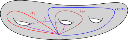
Figure 4. The curves $\alpha_{1}$, $\alpha_{2}$, $\alpha_{2}\alpha_{3}$ and $\gamma$ on a surface of genus 3

If $\eta=\alpha_{2}\alpha_{i}$, with $i\geqslant 4$, then, since $\rho$ and $\sigma$ agree on $\braket{\alpha_{1},\alpha_{2},\alpha_{3}}$ and are conjugate on $\braket{\eta,\alpha_{2},\alpha_{1}}$, Lemma 7.5 implies that they agree on $\eta$ and hence on $\alpha_{2}^{-1}\eta=\alpha_{i}$. Similarly, if $\eta=\alpha_{2}\beta_{i}^{-1}$, with $i\geqslant 3$, we can use Lemma 7.5 to show that $\rho$ and $\eta$ agree on $\eta$ and hence on $\beta_{i}$.

It remains to check that $\rho$ and $\sigma$ agree on $\beta_{1}$ and $\beta_{2}$. Recall that there exists a homeomorphism $h:S\to S$ so that $h\circ\alpha_{i}=\beta_{i}$ and $h\circ\beta_{i}=\alpha_{i}$. Then $\hat{\rho}=\rho\circ h_{*}$ and $\hat{\sigma}=\sigma\circ h_{*}$ are Hitchin representations. The above argument shows that $\hat{\rho}$ and $\hat{\sigma}$ are conjugate on $\braket{\alpha_{1},\alpha_{2},\alpha_{3},\beta_{3}}$, which implies that $\rho$ and $\sigma$ are conjugate on $\braket{\beta_{1},\beta_{2},\beta_{3},\alpha_{3}}$. Since $\rho$ and $\sigma$ agree on $\alpha_{3}$ and on $\beta_{3}\alpha_{3}\beta_{3}^{-1}$ (which have non-intersecting axes), Lemma 7.5 implies that $\rho$ and $\sigma$ agree on $\beta_{1}$ and $\beta_{2}$, which completes the proof. ∎

10. Infinitesmal Simple Length Rigidity

In this section, we prove that the differentials of simple length functions generate the cotangent space of a Hitchin component. In earlier work [7, Prop. 10.3] we showed that the differentials of all length functions generate the cotangent space, and that result played a key role in the proof that the pressure metric on the Hitchin component is non-degenerate.

Proposition 10.1.

Suppose that $S$ is a closed orientable surface of genus greater than 2 and $\rho\in{\mathcal{H}}_{d}(S)$. If $v\in\mathsf{T}_{\rho}({\mathcal{H}}_{d}(S))$ and ${\rm D}L_{\alpha}(v)=0$ for every simple non-separating curve $\alpha$, then $v=0$.

Moreover, if ${\rm D}\operatorname{Tr}_{\alpha}(v)=0$ for every simple non-separating curve $\alpha$, then $v=0$.

Proof.

We recall that there exists a component ${\widetilde{\mathcal{H}}}_{d}(S)$ of ${\rm Hom}(\pi_{1}(S),\mathsf{SL}_{d}(\mathbb{R}))$ which is an analytic manifold, so that the projection map $\pi:{\widetilde{\mathcal{H}}}_{d}(S)\to{\mathcal{H}}_{d}(S)$ is real analytic and is obtained by quotienting out by the action of $\mathsf{SL}_{d}(\mathbb{R})$ by conjugation, see Hitchin [20]. Any smooth path in ${\mathcal{H}}_{d}(S)$ lifts to a smooth path in ${\widetilde{\mathcal{H}}}_{d}(S)$. The real-valued functions $\widetilde{\operatorname{Tr}}_{\alpha}$ and $\widetilde{\lambda}_{i,\alpha}$ on ${\widetilde{\mathcal{H}}}_{d}(S)$ given by $\widetilde{\operatorname{Tr}_{\alpha}}(\tilde{\rho})=\operatorname{Tr}(\tilde{\rho}(\alpha))$ and $\widetilde{\lambda_{i,\alpha}}(\tilde{\rho})=\lambda_{i}(\tilde{\rho}(\alpha))$ are analytic and $\mathsf{SL}_{d}(\mathbb{R})$-invariant, so descend to real analytic functions $\operatorname{Tr}_{\alpha}$ and $\lambda_{i,\alpha}$ on ${\mathcal{H}}_{d}(S)$. (Notice that if we chose a different component of ${\rm Hom}(\pi_{1}(S),\mathsf{SL}_{d}(\mathbb{R}))$ as ${\widetilde{\mathcal{H}}}_{d}(S)$, then $\operatorname{Tr}_{\alpha}$ and $\lambda_{i,\alpha}$ could differ up to sign.)

The proof of Proposition 10.1 has the same basic structure as the proof of our simple length rigidity result. We first establish an infinitesimal version of Theorem 6.1.

Lemma 10.2.

If $S$ is a closed orientable surface of genus more than 1, $\rho\in{\mathcal{H}}_{d}(S)$ and $v\in\mathsf{T}{\mathcal{H}}_{d}(S)$ then ${\rm D}L_{\alpha}(v)=0$ for every simple non-separating curve $\alpha$ if and only if ${\rm D}\operatorname{Tr}_{\alpha}(v)=0$ for every simple non-separating curve $\alpha$. In both cases ${\rm D}\lambda_{i,\alpha}(v)=0$ for all $i$.

Proof.

Let $\{\rho_{t}\}_{t\in(-1,1)}$ be an analytic path in ${\widetilde{\mathcal{H}}}_{d}(S)$ such that if $\mathrel{\mathop{\rho}\limits^{\vbox to0.0pt{\kern-2.0pt\hbox{$\scriptstyle\bullet$}\vss}}}\!\!_{0}=\frac{{\rm d}}{{\rm d}t}\big{|}_{t=0}\rho_{t}$ then $d\pi(\mathrel{\mathop{\rho}\limits^{\vbox to0.0pt{\kern-2.0pt\hbox{$\scriptstyle\bullet$}\vss}}}\!\!_{0})=v$.

First assume that ${\rm D}L_{\alpha}(v)=0$ for every simple non-separating curve $\alpha$. Choose a simple based loop $\beta$ which intersects $\alpha$ only at the basepoint and has geometric intersection one with $\alpha$. Let $A(t)=\rho_{t}(\alpha)$, $B(t)=\rho_{t}(\beta)$ and $\lambda_{i}(t)=\lambda_{i,\alpha}(\rho_{t})$. Let $\lambda(n,t)=|\lambda_{1}(A(t)^{n}B(t))|$ and notice that our assumptions imply that

$$\mathrel{\mathop{\lambda}\limits^{\vbox to0.0pt{\kern-2.0pt\hbox{$\scriptstyle\bullet$}\vss}}}\!\!(n,0)=\frac{{\rm d}}{{\rm d}t}\Big{|}_{t=0}\lambda(n,t)=0$$

for all $n$. Let $(b^{i}_{j}(t))$ be the matrix representative of $B(t)$ in the basis $\{e_{i}(A(t))\}$ and notice that we may choose $\{e_{i}(A(t))\}$ to vary analytically, so that the coefficients $(b^{i}_{j}(t))$ vary analytically.

If $v\in\mathbb{R}^{d-1}$, let $D(v)\in\mathsf{SL}_{d}(\mathbb{R})$ be chosen so that its matrix is diagonal with respect to the basis $\{e_{i}(A(t))\}$ with diagonal entries $(1,v_{1},\ldots,v_{d-1})$, then $M(v,t)=D(v)B(t)$ depends analytically on $v$ and $t$. Notice that $M(\vec{0},0)$ has a simple eigenvalue $b^{1}_{1}(0)$ with eigenvector $e_{1}$. By Lemma 5.3 there exists an open neighborhood $V$ of the origin in $\mathbb{R}^{d-1}\times\mathbb{R}$ and an an analytic function $F:V\to\mathbb{R}$ so that

$$\lambda_{1}(M(v,t))=F(v,t).$$

Since

$$\frac{A(t)^{n}B(t)}{\lambda_{1}(t)^{n}}=M\left(\left(\frac{\lambda_{2}(t)}{\lambda_{1}(t)}\right)^{n},\ldots,\left(\frac{\lambda_{d}(t)}{\lambda_{1}(t)}\right)^{n},t\right)$$

and

$$\left(\left(\frac{\lambda_{2}(t)}{\lambda_{1}(t)}\right)^{n},\ldots,\left(\frac{\lambda_{d}(t)}{\lambda_{1}(t)}\right)^{n},t\right)\in V,$$

for all sufficiently large $n$ and $t$ sufficiently close to 0,

$$\frac{\lambda(n,t)}{\lambda_{1}(t)^{n}}=\frac{\lambda_{1}(A^{n}(t)B(t))}{\lambda_{1}(t)^{n}}=\lambda_{1}\left(\frac{A^{n}(t)B(t)}{\lambda_{1}(t)^{n}}\right)=F\left(\left(\frac{\lambda_{2}(t)}{\lambda_{1}(t)}\right)^{n},\ldots,\left(\frac{\lambda_{d}(t)}{\lambda_{1}(t)}\right)^{n},t\right).$$

Letting $u_{i}(t)=\frac{\lambda_{i+1}(t)}{\lambda_{1}(t)}$, we see that

$$\lambda(n,t)=\lambda_{1}(t)^{n}F\left(u_{1}(t)^{n},\ldots,u_{d-1}(t)^{n},t\right).$$

Since $\mathrel{\mathop{\lambda}\limits^{\vbox to0.0pt{\kern-2.0pt\hbox{$\scriptstyle\bullet$}\vss}}}\!\!_{1}(0)=0$ and $\mathrel{\mathop{\lambda}\limits^{\vbox to0.0pt{\kern-2.0pt\hbox{$\scriptstyle\bullet$}\vss}}}\!\!(n,0)=0$,

$$\frac{{\rm d}}{{\rm d}t}\Big{|}_{t=0}F\left(u_{1}(t)^{n},\ldots,u_{d-1}(t)^{n},t\right)=0$$

for all large enough $n$. Therefore,

$$\frac{\partial F}{\partial t}(u_{1}(0)^{n},\ldots,u_{d-1}(0)^{n},0)+\sum_{i=1}^{d-1}\frac{\partial F}{\partial v_{i}}(u_{1}(0)^{n},\ldots,u_{d-1}(0)^{n},0)nu_{i}^{n-1}(0)\mathrel{\mathop{u}\limits^{\vbox to0.0pt{\kern-2.0pt\hbox{$\scriptstyle\bullet$}\vss}}}\!\!_{i}(0)=0,$$ (7)

for all large enough $n$, so

$$\frac{\partial F}{\partial t}(0,\ldots,0,0)=0.$$

Moreover, since $\frac{\partial F}{\partial t}$ is analytic,

$$\frac{\partial F}{\partial t}(u_{1}(0)^{n},\ldots,u_{d-1}(0))^{n},0)=\sum_{i=1}^{d-1}\left(\frac{\partial^{2}F}{\partial v_{i}\partial t}(\vec{0},0)u_{i}(0)^{n}+o(u_{i}(0)^{n})\right)$$

so, since $1>|u_{1}(0)|>|u_{i}(0)|>0$ for all $i\geqslant 2$,

$$\lim_{n\rightarrow\infty}\frac{1}{nu_{1}(0)^{n-1}}\frac{\partial F}{\partial t}(u_{1}(0)^{n},\ldots,u_{d-1}(0))^{n},0)=\lim_{n\rightarrow\infty}\sum_{i=1}^{d-1}\frac{u_{i}(0)^{n}}{nu_{1}(0)^{n-1}}\left(\frac{\partial^{2}F}{\partial v_{i}\partial t}(0,\ldots,0,0)\right)=0$$

Equation (7) then implies that

$$\lim_{n\rightarrow\infty}\frac{1}{nu_{1}(0)^{n-1}}\left(\sum_{i=1}^{d-1}\frac{\partial F}{\partial v_{i}}(u_{1}(0)^{n},\ldots,u_{d-1}(0))^{n},0)nu_{i}^{n-1}(0)\mathrel{\mathop{u}\limits^{\vbox to0.0pt{\kern-2.0pt\hbox{$\scriptstyle\bullet$}\vss}}}\!\!_{i}(0)\right)=\frac{\partial F}{\partial v_{1}}(0,\ldots,0,0)\mathrel{\mathop{u}\limits^{\vbox to0.0pt{\kern-2.0pt\hbox{$\scriptstyle\bullet$}\vss}}}\!\!_{1}(0)=0$$

As in the proof of Lemma 5.1, we calculate that

$$\frac{\partial F}{\partial v_{1}}(0,\ldots,0,0)=\frac{{\rm d}}{{\rm d}s}\Big{|}_{s=0}F(s,0,\ldots,0)=\frac{{\rm d}}{{\rm d}s}\Big{|}_{s=0}\lambda_{1}\left(D(1,s,0,\ldots,0)B(0)\right)=\frac{{\rm d}}{{\rm d}s}\Big{|}_{s=0}\lambda_{1}\left(\begin{bmatrix}b^{1}_{1}(0)&b^{1}_{2}(0)\\ sb^{2}_{1}(0)&sb^{2}_{2}(0)\end{bmatrix}\right),$$

so

$$\frac{\partial F}{\partial v_{1}}(\vec{0},0)=\frac{b^{1}_{2}(0)b^{2}_{1}(0)}{b^{1}_{1}(0)}.$$

Lemma 6.4 implies that $b_{1}^{1}(0)$, $b_{2}^{1}(0)$ and $b_{1}^{2}(0)$ are non-zero, so $\frac{\partial F}{\partial v_{1}}(0,\ldots,0,0)\neq 0$. Therefore, $\mathrel{\mathop{u}\limits^{\vbox to0.0pt{\kern-2.0pt\hbox{$\scriptstyle\bullet$}\vss}}}\!\!_{1}(0)=0$ and, since $\mathrel{\mathop{\lambda}\limits^{\vbox to0.0pt{\kern-2.0pt\hbox{$\scriptstyle\bullet$}\vss}}}\!\!_{1}(0)=0$, we have

$$0=\mathrel{\mathop{u}\limits^{\vbox to0.0pt{\kern-2.0pt\hbox{$\scriptstyle\bullet$}\vss}}}\!\!_{1}(0)=\frac{{\rm d}}{{\rm d}t}\Bigg{|}_{t=0}\left(\frac{\lambda_{2}(t)}{\lambda_{1}(t)}\right)=\frac{\mathrel{\mathop{\lambda}\limits^{\vbox to0.0pt{\kern-2.0pt\hbox{$\scriptstyle\bullet$}\vss}}}\!\!_{2}(0)\lambda_{1}(0)-\mathrel{\mathop{\lambda}\limits^{\vbox to0.0pt{\kern-2.0pt\hbox{$\scriptstyle\bullet$}\vss}}}\!\!_{1}(0)\lambda_{2}(0)}{\lambda_{1}(0)^{2}}=\frac{\mathrel{\mathop{\lambda}\limits^{\vbox to0.0pt{\kern-2.0pt\hbox{$\scriptstyle\bullet$}\vss}}}\!\!_{2}(0)}{\lambda_{1}(0)},$$

so $\mathrel{\mathop{\lambda}\limits^{\vbox to0.0pt{\kern-2.0pt\hbox{$\scriptstyle\bullet$}\vss}}}\!\!_{2}(0)=0$.

We may iteratively consider the 1-parameter families of representations given by $\{E^{k}(\rho_{t})\}$ and apply the same analysis to conclude that $\mathrel{\mathop{\lambda}\limits^{\vbox to0.0pt{\kern-2.0pt\hbox{$\scriptstyle\bullet$}\vss}}}\!\!_{i,\alpha}(0)=0$ for all $i$, and thus that $D\operatorname{Tr}_{\alpha}(v)=0$.

Now assume that $D\operatorname{Tr}_{\alpha}(v)=0$ for every $\alpha\in\pi_{1}(S)$ represented by a simple non-separating curve. Given a simple, non-separating curve $\alpha$ represented by a simple based loop, we again choose a simple based loop $\beta$ which intersects $\alpha$ only at the basepoint and has geometric intersection one with $\alpha$. Notice that

$$Tr(\rho_{t}(\alpha^{n}\beta))=\sum_{i=1}^{d}\lambda_{i}^{n}(\rho_{t}(\alpha))\operatorname{Tr}({\bf{p}}_{i}(\rho_{t}(\alpha))\rho_{t}(\beta))=\sum_{i=1}^{d}h_{i}(t)\lambda_{i}^{n}(t).$$

where $h_{i}(t)=\operatorname{Tr}({\bf{p}}_{i}(\rho_{t}(\alpha))\rho_{t}(\beta))\neq 0$ for all $t$. Differentiating, and noting that $D\operatorname{Tr}_{\alpha^{n}\beta}(v)=0$ for all $n$, we see that

$$0=\sum_{i=1}^{d}\mathrel{\mathop{h}\limits^{\vbox to0.0pt{\kern-2.0pt\hbox{$\scriptstyle\bullet$}\vss}}}\!\!_{i}(0)\lambda_{i}^{n}(0)+nh_{i}(0)\mathrel{\mathop{\lambda}\limits^{\vbox to0.0pt{\kern-2.0pt\hbox{$\scriptstyle\bullet$}\vss}}}\!\!_{i}(0)\lambda_{i}(0)^{n-1}$$

for all $n$. Since $h_{i}(0)\neq 0$ and $\lambda_{i}(0)\neq 0$, it must be that $\mathrel{\mathop{h}\limits^{\vbox to0.0pt{\kern-2.0pt\hbox{$\scriptstyle\bullet$}\vss}}}\!\!_{1}(0)=0$ and $\mathrel{\mathop{\lambda}\limits^{\vbox to0.0pt{\kern-2.0pt\hbox{$\scriptstyle\bullet$}\vss}}}\!\!_{1}(0)=0$, so $DL_{\alpha}(v)=0$. ∎

We next generalize the proof of Theorem 7.1 to obtain a criterion guaranteeing that $v$ is infinitesmally trivial on its restriction to certain $3$-generator subgroups.

Lemma 10.3.

Suppose that $\rho\in{\mathcal{H}}_{d}(S)$, $v\in\mathsf{T}_{\rho}({\mathcal{H}}_{d}(S))$ and ${\rm D}L_{\eta}(v)=0$ for every simple non-separating curve $\eta$ on $S$. If $\alpha,\beta,\delta\in\pi_{1}(S)$ are represented by simple based loops which intersect only at the basepoint, and are freely homotopic to a collection of mutually disjoint and non-parallel, non-separating closed curves which do not bound a pair of pants in $S$, and $\{\rho_{t}\}$ is a path in ${\widetilde{\mathcal{H}}}_{d}(S)$ so that ${\rm D}\pi(\mathrel{\mathop{\rho}\limits^{\vbox to0.0pt{\kern-2.0pt\hbox{$\scriptstyle\bullet$}\vss}}}\!\!_{0})=v$, then there exists a path $\{C_{t}\}$ in $\mathsf{SL}_{d}(\mathbb{R})$, so that $C_{0}=I$ and if $\eta\in\braket{\alpha,\beta,\delta}$, then

$$\frac{{\rm d}}{{\rm d}t}\Big{|}_{t=0}(C_{t}\rho_{t}(\eta)C_{t}^{-1})=0\in\mathfrak{sl}(n,\mathbb{R}).$$

Proof.

Lemma 7.2 guarantees that there exist based loops $\hat{\alpha}$, $\hat{\beta}$, $\gamma$ and $\hat{\delta}$ as in Figure 1, which intersect only at the basepoint, so that $\hat{\alpha}$, $\hat{\beta}$ and $\hat{\delta}$ are freely homotopic to a collection of mutually disjoint, non-parallel, non-separating curves and $\gamma$ has geometric intersection one with each such that

$$\braket{\alpha,\beta,\delta}=\braket{\hat{\alpha},\hat{\beta},\hat{\delta}}.$$

We may thus assume that $\alpha$, $\beta$ and $\delta$ already have this form.

We may also, by possibly re-ordering $\alpha$, $\beta$ and $\delta$, assume that $\alpha^{p}\beta^{q}\gamma\delta^{r}$ is represented by a simple non-separating curve for all $p,q,r\in\mathbb{Z}$. We next generalize the proof of Proposition 7.3 to show that ${\rm D}\left(\frac{{\bf T}_{i,j,k}(\alpha,\beta,\delta)}{{\bf T}_{j,k}(\beta,\delta)}\right)(v)=0$ for all $i$, $j$ and $k$.

Recall that

$$\operatorname{Tr}(\rho(\alpha^{p}\beta^{q}\gamma\delta^{r}))=\sum_{i=1}^{d}\lambda_{i,\alpha}(\rho)^{p}\operatorname{Tr}\left({\bf{p}}_{i}(\rho(\alpha))\rho(\beta^{q}\gamma\delta^{r})\right).$$

Differentiating and noting that, by Lemma 10.2, ${\rm D}\operatorname{Tr}_{\alpha^{p}\beta^{q}\gamma\delta^{r}}(v)=0$ for all $p$, $q$ and $r$ and ${\rm D}\lambda_{i,\alpha}(v)=0$ for all $i$, one sees that

$$\sum_{i=1}^{d}\lambda_{i,\alpha}(\rho)^{p}{\rm D}{\bf T}_{i,0}(\alpha,\beta^{q}\gamma\delta^{r})(v)=0$$

for all $p$. By examining terms of different orders and taking limits, we see that

$${\rm D}{\bf T}_{i,0}(\alpha,\beta^{q}\gamma\delta^{r})(v)=0$$

for all $i$, $q$ and $r$. Repeating, as in the proof of Proposition 7.3, we find that

$${\rm D}{\bf T}_{i,j,0,k}(\alpha,\beta,\gamma,\delta)(v)=0$$

for all $i$, $j$, and $k$. Similarly, by considering $\beta^{q}\gamma\delta^{r}$, we see that

$${\rm D}{\bf T}_{j,0,k}(\beta,\gamma,\delta)(v)=0$$

for all $j$ and $k$.

Recall, from part (4) of Proposition 4.3, that

$${\bf T}_{i,j,0,k}(\alpha,\beta,\gamma,\delta)(\rho)={\bf T}_{j,0,k}(\beta,\gamma,\delta)(\rho)\left(\frac{{\bf T}_{i,j,k}(\alpha,\beta,\delta)(\rho)}{{\bf T}_{j,k}(\beta,\delta)(\rho)}\right)\neq 0$$

for all $i$, $j$ and $k$. Since we have established that the two leftmost terms in this expression are non-zero and have derivative $0$ in the direction $v$, we conclude that

$${\rm D}\left(\frac{{\bf T}_{i,j,k}(\alpha,\beta,\delta)}{{\bf T}_{j,k}(\beta,\delta)}\right)(v)=0$$

for all $i$, $j$ and $k$.

Let $a_{i}(t)=e_{i}(\rho_{t}(\alpha))$, $a^{i}(t)=e^{i}(\rho_{t}(\alpha))$, $b_{j}(t)=e_{j}(\rho_{t}(\beta))$, $b^{j}(t)=e^{j}(\rho_{t}(\beta))$, $d_{k}(t)=e_{k}(\rho_{t}(\delta))$ and $d^{k}(t)=e^{k}(\rho_{t}(\delta))$ for all $i,j,k$. We will assume throughout, by replacing $\{\rho_{t}\}$ by $\{C_{t}\rho_{t}C_{t}^{-1}\}$ where $\{C_{t}\}$ is a path in $\mathsf{SL}_{d}(\mathbb{R})$ so that $C_{0}=I$, that $a_{i}(t)$ are constant as functions of $t$ for all $i$, $b_{1}(t)$ is constant as a function of $t$, and by scaling the bases, that $\braket{a^{i}(t)}{b_{1}(t)}=1$ for all $i$ and $t$, $\braket{a^{1}(t)}{b_{j}(t)}=1$ for all $j$ and $t$, and $\braket{d^{k}(t)}{b_{1}(t)}=1$ for all $k$ and $t$. Since $a_{i}(t)$ is constant and $\frac{{\rm d}}{{\rm d}t}\big{|}_{t=0}\lambda_{i,\alpha}(\rho_{t})=0$, by Lemma 10.2, $\frac{{\rm d}}{{\rm d}t}\big{|}_{t=0}\rho_{t}(\alpha)=0$.

Recall, from Proposition 4.3, that

$$\frac{{\bf T}_{i,j,k}(\alpha,\beta,\delta)(\rho_{t})}{{\bf T}_{j,k}(\beta,\delta)(\rho_{t})}=\frac{\braket{a^{i}(t)}{b_{j}(t)}\braket{d^{k}(t)}{a_{i}(t)}}{\braket{d^{k}(t)}{b_{j}(t)}}.$$ (8)

By considering Equation (8) when $j=1$, we see that

$$\frac{{\bf T}_{i,1,k}(\alpha,\beta,\delta)(\rho_{t})}{{\bf T}_{1,k}(\beta,\delta)(\rho_{t})}=\braket{d^{k}(t)}{a_{i}(t)},$$

so, since the left-hand side has derivative 0 at 0 and $a_{i}(t)$ is constant for all $i$,

$$\frac{{\rm d}}{{\rm d}t}\Big{|}_{t=0}\big{(}\braket{d^{k}(t)}{a_{i}(t)}\big{)}=\braket{\mathrel{\mathop{d^{k}}\limits^{\vbox to0.0pt{\kern-2.0pt\hbox{$\scriptstyle\bullet$}\vss}}}\!\!(0)}{a_{i}(0)}=0$$

for all $i$ and $k$. Therefore, $\mathrel{\mathop{d^{k}}\limits^{\vbox to0.0pt{\kern-2.0pt\hbox{$\scriptstyle\bullet$}\vss}}}\!\!(0)=0$ for all $k$, so $\mathrel{\mathop{d}\limits^{\vbox to0.0pt{\kern-2.0pt\hbox{$\scriptstyle\bullet$}\vss}}}\!\!_{k}=0$ for all $k$. Since we also know, from Lemma 10.2, that $\frac{{\rm d}}{{\rm d}t}\big{|}_{t=0}\lambda_{i,\delta}(\rho_{t})=0$ for all $t$, it follows that $\frac{{\rm d}}{{\rm d}t}\big{|}_{t=0}\rho_{t}(\delta)=0$.

Considering Equation (8) when $i=1$, one obtains

$$\frac{{\bf T}_{1,j,k}(\alpha,\beta,\delta)(\rho_{t})}{{\bf T}_{j,k}(\beta,\delta)(\rho_{t})}=\frac{\braket{a^{1}(t)}{b_{j}(t)}\braket{d^{k}(t)}{a_{1}(t)}}{\braket{d^{k}(t)}{b_{j}(t)}}=\frac{\braket{d^{k}(t)}{a_{1}(t)}}{\braket{d^{k}(t)}{b_{j}(t)}}.$$

Since the derivative of the left hand side is 0 at 0, $a_{1}(t)$ is constant, and $\mathrel{\mathop{d^{k}}\limits^{\vbox to0.0pt{\kern-2.0pt\hbox{$\scriptstyle\bullet$}\vss}}}\!\!(0)=0$ for all $k$, we see that

$$\frac{\braket{d^{k}(0)}{a_{1}(0)}}{\braket{d^{k}(0)}{b_{j}(0)}^{2}}\braket{d^{k}(0)}{\mathrel{\mathop{b}\limits^{\vbox to0.0pt{\kern-2.0pt\hbox{$\scriptstyle\bullet$}\vss}}}\!\!_{j}(0)}=0,$$

so $\braket{d^{k}}{\mathrel{\mathop{b}\limits^{\vbox to0.0pt{\kern-2.0pt\hbox{$\scriptstyle\bullet$}\vss}}}\!\!_{j}(0)}=0$ for all $j$ and $k$, so $\mathrel{\mathop{b}\limits^{\vbox to0.0pt{\kern-2.0pt\hbox{$\scriptstyle\bullet$}\vss}}}\!\!_{j}(0)=0$ for all $j$. We may then argue, just as before, that $\frac{{\rm d}}{{\rm d}t}\big{|}_{t=0}\rho_{t}(\beta)=0$. Therefore, $\frac{{\rm d}}{{\rm d}t}\big{|}_{t=0}\rho_{t}(\eta)=0$ for all $\eta\in\braket{\alpha,\beta,\delta}$. ∎

We are now ready to complete the proof of Proposition 10.1. Let $\mathcal{S}=\{\alpha_{1},\beta_{1},\ldots,\alpha_{g},\beta_{g}\}$ be a standard generating set for $\pi_{1}(S)$. By Lemma 10.3, we may choose an analytic family $\{\rho_{t}\}$ in ${\rm Hom}(\pi_{1}(S),\mathsf{PSL}_{d}(\mathbb{R}))$ so that $d\pi(\mathrel{\mathop{\rho}\limits^{\vbox to0.0pt{\kern-2.0pt\hbox{$\scriptstyle\bullet$}\vss}}}\!\!_{0})=v$ and $\frac{{\rm d}}{{\rm d}t}\big{|}_{t=0}\rho_{t}(\gamma)=0$ for all $\eta\in\braket{\alpha_{1},\alpha_{2},\alpha_{3}}$.

For any $\delta\in\mathcal{S}-\{\alpha_{1},\alpha_{2},\alpha_{3},\beta_{1},\beta_{2}\}$, we may apply Lemma 10.3 to the triple $\{\alpha_{1},\alpha_{2},\eta\}$ to show that there exists a family $\{C_{t}\}$ in $\mathsf{PSL}_{d}(\mathbb{R})$ so that $C_{0}=I$ and $\frac{{\rm d}}{{\rm d}t}\big{|}_{t=0}(C_{t}\rho_{t}(\gamma)C_{t}^{-1})=0$ for all $\gamma\in\braket{\alpha_{1},\alpha_{2},\delta}$. In particular,

$$\mathrel{\mathop{C}\limits^{\vbox to0.0pt{\kern-2.0pt\hbox{$\scriptstyle\bullet$}\vss}}}\!\!_{0}\rho_{0}(\alpha_{i})C_{0}^{-1}-C_{0}\rho_{0}(\alpha_{i})\mathrel{\mathop{C}\limits^{\vbox to0.0pt{\kern-2.0pt\hbox{$\scriptstyle\bullet$}\vss}}}\!\!_{0}+C_{0}\left(\frac{{\rm d}}{{\rm d}t}\Big{|}_{t=0}\rho_{t}(\alpha_{i})\right)C_{0}^{-1}=\mathrel{\mathop{C}\limits^{\vbox to0.0pt{\kern-2.0pt\hbox{$\scriptstyle\bullet$}\vss}}}\!\!_{0}\rho_{0}(\alpha_{i})-\rho_{0}(\alpha_{i})\mathrel{\mathop{C}\limits^{\vbox to0.0pt{\kern-2.0pt\hbox{$\scriptstyle\bullet$}\vss}}}\!\!_{0}=0,$$

so $[\mathrel{\mathop{C}\limits^{\vbox to0.0pt{\kern-2.0pt\hbox{$\scriptstyle\bullet$}\vss}}}\!\!_{0},\rho_{0}(\alpha_{i})]=0$ for $i=1,2$, Thus, $\mathrel{\mathop{C}\limits^{\vbox to0.0pt{\kern-2.0pt\hbox{$\scriptstyle\bullet$}\vss}}}\!\!_{0}$ is diagonalizable over $\mathbb{R}$ with respect to both $\{e_{i}(\rho_{0}(\alpha_{1}))\}$ and $\{e_{i}(\rho_{0}(\alpha_{2})\}$.

If $\mathrel{\mathop{C}\limits^{\vbox to0.0pt{\kern-2.0pt\hbox{$\scriptstyle\bullet$}\vss}}}\!\!_{0}\neq 0$, then $\mathbb{R}^{d}$ admits a non-trivial decomposition into eigenspaces of $\mathrel{\mathop{C}\limits^{\vbox to0.0pt{\kern-2.0pt\hbox{$\scriptstyle\bullet$}\vss}}}\!\!_{0}$ with distinct eigenvalues. Any such eigenspace $W$ is spanned by a sub-collection of $\{e_{i}(\rho_{0}(\alpha_{1}))\}$ and by a sub-collection of $\{e_{j}(\rho_{0}(\alpha_{2}))\}$. In particular, some $e_{i}(\rho_{0}(\alpha_{1}))$ is in the sub-space spanned by a subcollection of $\{e_{j}(\rho_{0}(\alpha_{2}))\}$. Since $\alpha_{1}$ and $\alpha_{2}$ are disjoint curves, this contradicts Theorem 1.6. Therefore, $\mathrel{\mathop{C}\limits^{\vbox to0.0pt{\kern-2.0pt\hbox{$\scriptstyle\bullet$}\vss}}}\!\!_{0}=0$.

Since $\mathrel{\mathop{C}\limits^{\vbox to0.0pt{\kern-2.0pt\hbox{$\scriptstyle\bullet$}\vss}}}\!\!_{0}=0$ and $\frac{{\rm d}}{{\rm d}t}\big{|}_{t=0}(C_{t}\rho_{t}(\delta)C_{t}^{-1})=0$, we calculate that

$$\mathrel{\mathop{C}\limits^{\vbox to0.0pt{\kern-2.0pt\hbox{$\scriptstyle\bullet$}\vss}}}\!\!_{0}\rho_{0}(\delta)C^{-1}_{0}-C_{0}\rho_{0}(\delta)\mathrel{\mathop{C}\limits^{\vbox to0.0pt{\kern-2.0pt\hbox{$\scriptstyle\bullet$}\vss}}}\!\!_{0}+C_{0}\left(\frac{{\rm d}}{{\rm d}t}\Big{|}_{t=0}\rho_{t}(\delta)\right)C_{0}^{-1}=\frac{{\rm d}}{{\rm d}t}\Big{|}_{t=0}\rho_{t}(\delta)=0.$$

By considering the subgroups $\braket{\alpha_{2},\alpha_{3},\beta_{1}}$ and $\braket{\alpha_{1},\alpha_{3},\beta_{2}}$, we similarly show that

$$\frac{{\rm d}}{{\rm d}t}\Big{|}_{t=0}\rho_{t}(\beta_{1})=0\qquad{\rm and}\qquad\frac{{\rm d}}{{\rm d}t}\Big{|}_{t=0}\rho_{t}(\beta_{2})=0$$

Since $\frac{{\rm d}}{{\rm d}t}\big{|}_{t=0}\rho_{t}(\eta)=0$ for all $\eta\in\mathcal{S}$,

$$\mathrel{\mathop{\rho}\limits^{\vbox to0.0pt{\kern-2.0pt\hbox{$\scriptstyle\bullet$}\vss}}}\!\!_{0}=0\in\mathsf{T}{\widetilde{\mathcal{H}}}_{d}(S).$$

Therefore, $v={\rm D}\pi\left(\mathrel{\mathop{\rho}\limits^{\vbox to0.0pt{\kern-2.0pt\hbox{$\scriptstyle\bullet$}\vss}}}\!\!_{0}\right)=0$ as claimed. ∎

11. Hitchin representations for surfaces with boundary

In this section, we observe that our main simple length rigidity result extends to Hitchin representations of most compact surfaces with boundary.

If $S$ is a compact surface with boundary, we say that a representation $\rho:\pi_{1}(S)\to\mathsf{PSL}_{d}(\mathbb{R})$ is a Hitchin representation if $\rho$ is the restriction of a Hitchin representation $\hat{\rho}$ of $\pi_{1}(DS)$ into $\mathsf{PSL}_{d}(\mathbb{R})$, where $DS$ is the double of $S$. Labourie and McShane [23, Section 9] show that this is equivalent to assuming that $\rho$ is deformable to the composition of a convex cocompact Fuchsian uniformization of $S$ and the irreducible representation through representations so that the image of every peripheral element is purely loxodromic. (Recall that a non-trivial element of $\pi_{1}(S)$ is peripheral if it is represented by a curve in $\partial S$.) Fock and Goncharov [14] refer to such representations as positive representations.

Theorem 11.1.

Suppose that $S$ is a compact, orientable surface of genus $g>0$ with $p>0$ boundary components, and $(g,p)$ is not $(1,1)$ or $(1,2)$. If $\rho$ and $\sigma$ are two Hitchin representations of $\pi_{1}(S)$ of dimension $d$ and $L_{\rho}(\alpha)=L_{\sigma}(\alpha)$ for any $\alpha$ represented by a simple non-separating curve on $S$, then $\rho$ and $\sigma$ are conjugate in $\mathsf{PGL}_{d}(\mathbb{R})$.

Notice that our techniques don’t apply to punctured spheres, since they contain no simple non-separating curves. In the remaining excluded cases, there are no configurations of three non-parallel simple non-separating closed curves which do not bound a pair of pants.

Proof.

We choose a generating set

$$\mathcal{S}=\{\alpha_{1},\beta_{1},\ldots\alpha_{g},\beta_{g},\delta_{1},\ldots,\delta_{p-1}\}$$

represented by simple, non-separating based loops which intersect only at the basepoint so that $\{\alpha_{1},\beta_{1},\ldots,\alpha_{g},\beta_{g}\}$ is a standard generating set for the surface of genus $g$ obtained by capping each boundary component of $S$ with a disk, each $\delta_{i}$ has geometric intersection one with $\beta_{1}$ and zero with every other generator, as in Figure 5. Notice that any collection of 3 based loops in $\mathcal{S}$ which have geometric intersection zero with each other are freely homotopic to a mutually disjoint, non-parallel collection of simple closed curves which do not bound a pair of pants.

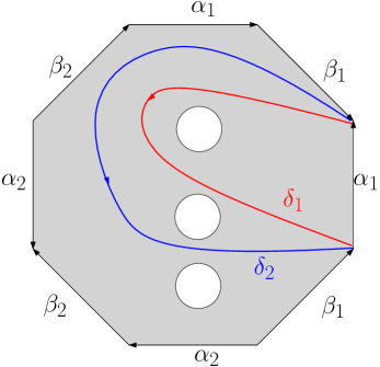
Figure 5. Our generators on a surface with genus 2 and 3 boundary components

Throughout the proof we identify $S$ with a subsurface of $DS$ and apply our earlier results to the representations $\hat{\rho}$ and $\hat{\sigma}$ of $\pi_{1}(DS)$. Lemma 6.3 implies that if $\eta\in\pi_{1}(S)$ is represented by a simple non-separating curve on $S$, then $|\operatorname{Tr}(\rho(\eta))|=|\operatorname{Tr}(\sigma(\eta))|$ and $\lambda_{i}(\rho(\eta))=\lambda_{i}(\sigma(\eta))$ for all $i$.

If $g\geqslant 3$, the proof of Theorem 1.2 generalizes rather immediately. We first apply Theorem 7.1 to $\hat{\rho}$ and $\hat{\sigma}$, to see that we may assume, after conjugation in $\mathsf{PGL}_{d}(\mathbb{R})$, that $\rho$ and $\delta$ agree on $\braket{\alpha_{1},\alpha_{2},\alpha_{3}}$. If $\eta\in\mathcal{S}-\{\alpha_{1},\alpha_{2},\beta_{1},\beta_{2}\}$, we may again apply Theorem 7.1 to show that $\rho$ and $\sigma$ are conjugate on $\braket{\alpha_{1},\alpha_{2},\eta}$. Since $\hat{\rho}$ and $\hat{\sigma}$ agree on $\alpha_{1}$ and $\alpha_{2}$, Lemma 7.5 implies that $\rho$ and $\sigma$ agree on $\braket{\alpha_{1},\alpha_{2},\eta}$. We then consider the triples $\{\alpha_{2},\alpha_{3},\beta_{1}\}$ and $\{\alpha_{1},\alpha_{3},\beta_{2}\}$ to show that $\rho$ and $\sigma$ agree on $\beta_{1}$ and $\beta_{2}$, and hence that $\rho=\sigma$.

If $g=2$ and $p\geqslant 2$, we again use Theorem 7.1 to show that we may conjugate $\rho$ and $\sigma$ so that they agree on $\braket{\alpha_{1},\alpha_{2},\delta_{1}}$. If $i\geqslant 2$, we may again apply Theorem 7.1 to show that $\rho$ and $\sigma$ are conjugate on $\braket{\alpha_{1},\alpha_{2},\delta_{i}}$ and then Lemma 7.5 to show that $\rho$ and $\sigma$ agree on $\braket{\alpha_{1},\alpha_{2},\delta_{i}}$. We consider the triple $\{\alpha_{1},\delta_{1},\beta_{2}\}$ to show that $\rho$ and $\sigma$ agree on $\beta_{2}$. Therefore, $\rho$ and $\sigma$ agree on $\mathcal{S}-\{\beta_{1}\}$. Recall that there exists a homeomorphism $h:S\to S$ such that $h\circ\alpha_{i}=\beta_{i}$ and $h\circ\beta_{i}=\alpha_{i}$. The above argument implies that the Hitchin representations $\rho\circ h_{*}$ and $\sigma\circ h_{*}$ are conjugate on $\braket{\alpha_{1},\alpha_{2},\beta_{2}}$ and hence that $\rho$ and $\sigma$ are conjugate on $\braket{\beta_{1},\beta_{2},\alpha_{2}}$. Since $\rho$ and $\sigma$ agree on $\beta_{2}$ and $\alpha_{2}$, Lemma 7.5 implies that they agree on $\beta_{1}$. So, we conclude that $\rho=\sigma$.

If $g=1$ and $p\geqslant 3$, then $\mathcal{S}=\{\alpha_{1},\beta_{1},\delta_{1},\ldots,\delta_{p-1}\}$. We first apply Theorem 7.1 to show that we may conjugate $\rho$ and $\sigma$ so that they agree on $\braket{\alpha_{1},\delta_{1},\delta_{2}}$. If $i\geqslant 3$, we may consider the triple $\{\alpha_{1},\delta_{1},\delta_{i}\}$ to see that $\rho$ and $\sigma$ agree on $\delta_{i}$. It remains to check that $\rho$ and $\sigma$ agree on $\beta_{1}$.

Figure 6. Curves on a surface of type $(1,p)$ for $p\geqslant 3$

Let $\hat{\delta}_{i}$ be as in Figure 6, so that if $\mathcal{S}^{\prime}=\{\alpha_{1},\beta_{1},\hat{\delta}_{1},\ldots,\hat{\delta}_{p-1}\}$, then the based loops in $\mathcal{S}^{\prime}$ intersect only at the basepoint and each $\hat{\delta}_{i}$ has geometric intersection one with $\alpha_{1}$ and has geometric intersection zero with every other element of $\mathcal{S}^{\prime}$. Notice that $\alpha_{1}\delta_{i}=\hat{\delta}_{i}\beta_{1}$ and let $u_{i}=\alpha_{1}\delta_{i}$. Then, $\rho$ and $\sigma$ agree on the subgroup $\braket{\alpha_{1},u_{1},\ldots,u_{p-1}}$. We may apply the same argument as above to show that $\rho$ and $\sigma$ are conjugate on $\braket{\beta_{1},\hat{\delta}_{1},\ldots,\hat{\delta}_{p-1}}$. Since this subgroup contains $u_{1}$ and $u_{2}$, $\rho$ and $\sigma$ agree on $u_{1}$ and $u_{2}$, and $u_{1}$ and $u_{2}$ have non-intersecting axes in $\pi_{1}(DS)$, Lemma 7.5, applied to $\hat{\rho}$ and $\hat{\sigma}$, implies that $\rho$ and $\sigma$ agree on $\braket{\beta_{1},\hat{\delta}_{1},\ldots,\hat{\delta}_{p-1}}$ and hence on $\beta_{1}$, so $\rho=\sigma$.

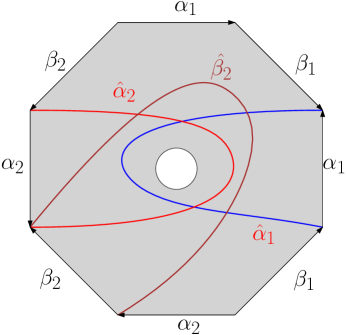
Figure 7. Genus 2 with 1 puncture

If $g=2$ and $p=1$, then $\mathcal{S}=\{\alpha_{1},\beta_{1},\alpha_{2},\beta_{2}\}$. We will consider the based loops $\hat{\alpha}_{i}$ and $\hat{\beta}_{i}$ as in Figure 7. As the based loops $\{\alpha_{1},\alpha_{2},\hat{\alpha}_{1}\}$ are freely homotopic to a mutually disjoint, non-parallel collection of simple, non-separating curves which do not bound a pair of pants, Theorem 7.1 implies that we may assume that $\rho$ and $\sigma$ agree on $\braket{\alpha_{1},\alpha_{2},\hat{\alpha}_{1}}$. Similarly, the representations are conjugate on $\braket{\alpha_{1},\alpha_{2},\hat{\alpha}_{2}}$, and since they already agree on $\braket{\alpha_{1},\alpha_{2},\hat{\alpha}_{1}}$ and $\alpha_{1}$ and $\alpha_{2}$ have non-intersecting axes, Lemma 7.5 implies that they agree on $\braket{\alpha_{1},\alpha_{2},\hat{\alpha}_{1},\hat{\alpha}_{2}}$. Next, by considering the triples $\{\alpha_{1},\beta_{2},\hat{\alpha}_{1}\}$ and $\{\alpha_{1},\beta_{2},\hat{\beta}_{2}\}$, we see that $\rho$ and $\sigma$ are conjugate on $\braket{\alpha_{1},\beta_{2},\hat{\alpha}_{1},\hat{\beta}_{2}}$. Since $\rho$ and $\sigma$ agree on $\alpha_{1}$ and $\hat{\alpha}_{1}$, they agree on $\braket{\alpha_{1},\beta_{2},\hat{\alpha}_{1},\hat{\beta}_{2}}$. By similarly considering the triples $\{\alpha_{2},\beta_{1},\hat{\alpha}_{2}\}$ and $\{\alpha_{2},\beta_{1},\hat{\beta}_{1}\}$, we show that $\rho$ and $\sigma$ agree on $\beta_{1}$. Since we have shown that, after an initial conjugation, $\rho$ and $\sigma$ agree on each generator, we have completed the proof in the case that $(g,p)=(2,1)$. ∎

We similarly obtain the analogue of our Simple Trace Rigidity Theorem in this setting.

Theorem 11.2.

Suppose that $S$ is a compact, orientable surface of genus $g>0$ with $p>0$ boundary components and $(g,p)$ is not $(1,1)$ or $(1,2)$. Then, for all $d\geqslant 2$, there exists a finite collection $\mathcal{L}_{d}(S)$ of elements of $\pi_{1}(S)$ which are represented by simple non-separating curves, such that if $\rho$ and $\sigma$ are two Hitchin representations of $\pi_{1}(S)$ of dimension $d$ and $|\operatorname{Tr}(\rho(\eta))|=|\operatorname{Tr}(\sigma(\eta))|$ for any $\eta\in\mathcal{L}_{d}(S)$, then $\rho$ and $\sigma$ are conjugate in $\mathsf{PGL}_{d}(\mathbb{R})$.

References

- [1]
- [2] Y. Benoist, “Convexes divisibles I,” in Algebraic groups and arithmetic, Tata Inst. Fund. Res. Stud. Math. 17(2004), 339–374.
- [3] F. Bonahon, “The geometry of Teichmüller space via geodesic currents,” Invent. Math. 92(1988), 139–162.
- [4] R. Bowen, “Periodic orbits of hyperbolic flows,” Amer. J. Math. 94 (1972), 1–30.
- [5] M. Bridgeman, “Hausdorff dimension and the Weil-Petersson extension to quasifuchsian space,” Geom. Top. 14(2010), 799–831.
- [6] M. Bridgeman and R. Canary, “Simple length rigidity for Kleinian surface groups and applications,” Comm. Math. Helv. 92(2017), 715–750.
- [7] M. Bridgeman, R. Canary, F. Labourie and A. Sambarino, “The pressure metric for Anosov representations,” G.A.F.A. 25(2015), 1089–1179.
- [8] M. Bridgeman, R. Canary and A. Sambarino, “An introduction to pressure metrics on higher Teichmüller spaces,” Erg. Thy. Dyn. Sys., to appear, preprint available at: https://arxiv.org/abs/1507.03894
- [9] V. Charette and T. Drumm, “Strong marked isospectrality of affine Lorentzian groups," J. Diff. Geom. 66(2004), 437–452.
- [10] S. Choi and W. Goldman, “Convex real projective structures on closed surfaces are closed,” Proc. A.M.S. 118(1993), 657–661.
- [11] D. Cooper and K. Delp, “The marked length spectrum of a projective manifold or orbifold,” Proc. of the A.M.S. 138(2010), 3361–3376.
- [12] F. Dal’Bo and I. Kim, “Marked length rigidity for symmetric spaces,” Comm. Math. Helv. 77(2002), 399–407.
- [13] M. Duchin, C. Leininger and K. Rafi, “ Length spectra and degeneration of flat metrics,”Invent. Math. 182(2010), 231–277.
- [14] V. Fock and A. Goncharov, “Moduli spaces of local systems and higher Teichmüller theory,” Publ. Math. I.H.E.S. 103(2006), 1–211.
- [15] S. Fomin and A. Zelevinsky, “Total positivity: tests and parameterizations,” Math. Intell. 22(2000), 23–33.
- [16] M. Gasca and J.M. Pena, “Total positivity and Neville elimination,” Lin. Alg. App. 165(1992), 25–44.
- [17] O. Guichard,“Zariski closures of positive and maximal representations,” in preparation.
- [18] O. Guichard and A. Wienhard, “Anosov representations: Domains of discontinuity and applications,” Invent. Math. 190(2012), 357–438.
- [19] U. Hamenstädt, “Length functions and parameterizations of Teichmüller space for surfaces with cusps,” Ann. Acad. Sci. Fenn. Math. 28(2003), 75–88.
- [20] N. Hitchin, “Lie groups and Teichmüller space,” Topology 31(1992), 449–473.
- [21] I. Kim, “Rigidity and deformation space of strictly convex real projective structures,” J. Diff. Geom. 58(2001), 189–218.
- [22] F. Labourie, “Anosov flows, surface groups and curves in projective space,” Invent. Math. 165(2006), 51–114.
- [23] F. Labourie and G. McShane, “Cross ratios and identities for higher Thurston theory,” Duke Math J. 148(2009), 279–345.
- [24] P. Lax, Linear Algebra, Wiley-Interscience, 1996.
- [25] G. Lusztig, “Total positivity in reductive groups,” in Lie Theory and Geometry: in honor of B. Kostant, Birkhäuser, 1994, 531–568.
- [26] G. Lusztig, “Total positivity in partial flag manifolds,” Rep. Thy. 2(1998), 70–78.
- [27] J. Marché and M. Wolff, “The modular action on -characters in genus 2,” Duke Math. J. 165(2016), 371–412.
- [28] G. Margulis, On some aspects of the theory of Anosov systems, Springer-Verlag, 2004.
- [29] H. Masur and M. Wolf, “The Weil-Petersson isometry group,” Geom. Ded. 93(2002), 177–190.
- [30] C. McMullen, “Thermodynamics, dimension and the Weil-Petersson metric,” Invent. Math. 173(2008), 365–425.
- [31] R. Potrie and A. Sambarino, “Eigenvalues and entropy of a Hitchin representation,” Invent. Math. 209(2017), 885–925.
- [32] H. Royden, “Automorphisms and isometries of Teichmüller spaces,” in Advances in the theory of Riemann surfaces, Annals of Math. Studies, Vol. 66(1970), 369–383.
- [33] A. Sambarino, “Quantitative properties of convex representations,” Comm. Math. Helv., 89(2014), 443–488.
- [34] P. Schmutz, “Die Parametrisierung des Teichmüllerraumes durch geodätische Längenfunktionen,” Comm. Math. Helv. 68(1993), 278–288.
- [35] S. Wolpert, “Thurston’s Riemannian metric for Teichmüller space,” J. Diff. Geom. 23(1986), 143–174.