Enhancing the Spectral Hardening of Cosmic TeV Photons by Mixing with Axionlike Particles in the Magnetized Cosmic Web

Abstract

Large-scale extragalactic magnetic fields may induce conversions between very-high-energy photons and axionlike particles (ALPs), thereby shielding the photons from absorption on the extragalactic background light. However, in simplified “cell” models, used so far to represent extragalactic magnetic fields, this mechanism would be strongly suppressed by current astrophysical bounds. Here we consider a recent model of extragalactic magnetic fields obtained from large-scale cosmological simulations. Such simulated magnetic fields would have large enhancement in the filaments of matter. As a result, photon-ALP conversions would produce a significant spectral hardening for cosmic TeV photons. This effect would be probed with the upcoming Cherenkov Telescope Array detector. This possible detection would give a unique chance to perform a tomography of the magnetized cosmic web with ALPs.

Introduction—Axionlike particles (ALPs) are ultralight pseudoscalar bosons $a$ with a two-photon vertex $a\gamma\gamma$, predicted by several extensions of the Standard Model (see Jaeckel:2010ni for a recent review). In the presence of an external magnetic field, the $a\gamma\gamma$ coupling leads to the phenomenon of photon-ALP mixing Raffelt:1987im . This effect allows for the possibility of direct searches of ALPs in laboratory experiments. In this respect a rich, diverse experimental program is being carried out, exploiting different sources and approaches Ehret:2010mh ; Arik:2015cjv ; Duffy:2006aa . See Graham:2015ouw for a review.

Because the $a\gamma\gamma$ coupling, ultralight ALPs can also play an important role in astrophysical observations. In particular, an intriguing hint for ALPs has been recently suggested by very-high-energy (VHE) $\gamma$-ray experiments. In this respect, recent observations of cosmologically distant $\gamma$-ray sources by ground-based $\gamma$-ray Imaging Atmospheric Cherenkov Telescopes have revealed a surprising degree of transparency of the Universe to VHE photons Aharonian:2005gh ; Horns:2012fx , where one would have expected a significant absorption of VHE photons by pair-production processes ($\gamma_{\rm VHE}+\gamma_{\rm EBL}\to e^{+}e^{-}$) on the extragalactic background light (EBL). Even though this problem has been also analyzed using more conventional physics (see, e.g., Essey:2009zg ; Essey:2009ju ), photon-ALP oscillations in large-scale magnetic fields provide a natural mechanism to drastically reduce the photon absorption Csaki:2003ef ; De Angelis:2007dy ; Simet:2007sa ; Dominguez:2011xy ; DeAngelis:2011id ; Horns:2012kw ; Meyer:2013pny ; Troitsky:2015nxa . In order to have efficient conversions one should achieve the strong-mixing regime which is realized above a critical energy given by DeAngelis:2007wiw

$$E_{c}\simeq\frac{500\,\ m_{a}^{2}}{(10^{-9}\,\ \textrm{eV})^{2}}\left(\frac{10^{-9}\,\ \textrm{G}}{B_{T}}\right)\left(\frac{5\times 10^{-11}}{g_{a\gamma}}\right)\,\ \textrm{GeV}\,\ .$$ (1)

In the previous expression one typically considers $g_{a\gamma}\lesssim 5\times 10^{-11}$ GeV^-1 in order to be consistent with the bounds from the helioscope experiment CAST at CERN Arik:2015cjv ; Castcant , and from energy loss in globular-clusters stars Ayala:2014pea that give $g_{a\gamma}\lesssim 6\times 10^{-11}$ GeV^-1 (see Fig. 1). Notably two mechanisms have been proposed in order to reduce the cosmic opacity through conversions into ALPs. The first involves extragalactic magnetic fields De Angelis:2007dy . At present, the lowest upper limits on extragalactic magnetic fields on the largest cosmological scales come from cosmic microwave background observations  Planck2015 and from Faraday rotation measurements of polarized extragalactic sources  Blasi:1999hu and are compatible with an average field strength of $B\lesssim{\mathcal{O}}(1$ nG) with a coherence length $l_{c}\sim{\mathcal{O}}(1$ Mpc) Pshirkov:2015tua . In this case, in order to have sizeable conversions into ALPs at $E\gtrsim 100$ GeV, one should consider $m_{a}\lesssim 10^{-9}\,\ \textrm{eV}$. In the second scenario, one requires strong photon conversions in the magnetic fields of the source and back-conversions in the Milky Way Simet:2007sa . Estimates on the Galactic magnetic field of order $B\sim{\mathcal{O}}(10^{-6}$ G) are obtained by measurements of the Faraday Rotation Jansson:2012pc ; Pshirkov:2011um ; Oppermann:2011td ; Mao:2010zr . In this case, one expects significant conversions for $m_{a}\lesssim 10^{-8}\,\ \textrm{eV}$. The resultant parameter space where ALPs would explain the low $\gamma$-ray opacity under these conditions is shown in light blue Meyer:2013pny in Fig. 1.

However, the range of the parameters where ALPs would impact the cosmic transparency is constrained from other observations, as shown in Fig. 1. In particular, for ALPs with masses $m_{a}\lesssim 10^{-9}$ eV, the strongest bound on $g_{a\gamma}$ is derived from the absence of $\gamma$-rays from SN 1987A. In this regard, a recent analysis results in $g_{a\gamma}<5\times 10^{-12}$ GeV^-1 for $m_{a}\lesssim 10^{-10}$ eV Payez:2014xsa . A comparable bound on $g_{a\gamma}$ has been recently extended in the mass range $0.5\lesssim m_{a}\lesssim 5$ neV from the nonobservation in Fermi Large Array Telescope (LAT) data of irregularities induced by photon-ALP conversions in the $\gamma$-ray spectrum of NGC 1275, the central galaxy of the Perseus Cluster TheFermi-LAT:2016zue . It is worth mentioning that from the absence of x-ray spectral modulations in active galactic nuclei, for $m_{a}\lesssim 10^{-12}\,\ \textrm{eV}$ we have a stronger bound on the coupling: $g_{a\gamma}\lesssim 1\times 10^{-12}$ GeV^-1 Berg:2016ese ; Conlon:2017qcw . However, in the following we will always refer to higher ALP masses. Data from the H.E.S.S. observations of the distant BL Lac object PKS 2155-304 also limit $g_{a\gamma}<2.1\times 10^{-11}$ GeV^-1 for $15\lesssim m_{a}\lesssim 60$ neV Abramowski:2013oea . Therefore, while the mechanism of conversions into the Galactic magnetic field is still valid at $m_{a}\lesssim 10^{-8}\,\ \textrm{eV}$, the conversions into the extragalactic magnetic field seem strongly disfavored as a mechanism to reduce the cosmic opacity. However, the distribution of the extragalactic magnetic fields has been oversimplified in previous works on ALP conversions. In particular, a cell-like structure (hereafter named the “cell” model) has been adopted with many domains of equal size ($l_{c}\sim 1$ Mpc) in which the magnetic field has (constant) random values and directions De Angelis:2007dy . Only recently it has been pointed out that in more realistic situations, the magnetic field direction would vary continuously along the propagation path, and this would lead to sizeable differences in the ALP conversions with respect to the “cell” model Angus:2013sua ; Wang:2015dil ; Kartavtsev:2016doq ; Masaki:2017aea . Here we study for the first time the photon conversions into ALPs using recent magneto-hydrodynamical cosmological simulations Vazza14 ; Gheller16 , which represent a step forward in the realistic modeling of cosmic magnetism. In this more realistic case the magnetic fields can locally fluctuate in filaments of matter up to 2 orders of magnitude larger that found in the “cell” model and photon-ALP conversions are enhanced compared to previous estimates. Indeed, significant conversions are found both in the low-mass region (indicated as “LM,” $m_{a}\lesssim 10^{-10}$ eV) below the SN 1987A bound and in the high-mass region (“HM,” $m_{a}\gtrsim 10^{-8}$ eV) on the right of the recent Fermi-LAT bound. These two ranges are indicated with small squares in Fig. 1 and represent regions of sensitivity (see Supplemental Material for details). We have also checked that for these parameters possible photon-ALP conversions at relatively high redshifts do not distort the cosmic microwave background Mirizzi:2005ng . Therefore, our new model significantly enlarges the parameter space where the photon-ALP conversions would reduce the cosmic opacity, as shown in Fig. 1 where we compare the photon transfer function $T_{\gamma}$ in presence of ALP conversions for the cell model and for the simulated model of extragalactic $B$-field (see Supplemental Material for details). In particular, these values of ALPs parameters are in the reach of the planned upgrade of the photon regeneration experiment ALPS at DESY Ehret:2010mh and with the next generation solar axion detector IAXO (International Axion Observatory) Irastorza:2011gs (see Fig. 1) or with Fermi-LAT if luckily a galactic supernova would explode in its field of view Meyer:2016wrm .

Figure 1: Limits on ALP parameter space in the plane $(m_{a},g_{a\gamma})$. The parameter space where ALPs could explain the low $\gamma$-ray opacity is shown in light blue Meyer:2013pny . The horizontal grey bands represent the sensitivity of future ALPS-II and IAXO experiments. Dashed lines represent the photon transfer function $T_{\gamma}$ for the cell model and simulated model of the extragalactic $B$-field. The two small squares represent cases of low-mass and high-mass ALPs where conversions in simulated extragalactic magnetic fields would affect the TeV photon transparency. (See text for details.)

Simulated extragalactic magnetic fields—Our recent model for extragalactic magnetic fields comes from a suite of simulations Vazza14 produced using the cosmological code ENZO Enzo14 , with the magnetohydrodynamical method outlined in Wang09 . These simulations are nonradiative and evolved a uniform primordial seed field of $B_{0}=1~{}\rm nG$ (comoving) for each component, starting from $z=38$ and for a comoving volume of $200^{3}\rm Mpc^{3}$, sampled using a fixed grid of $2400^{3}$ cells (for the fixed comoving resolution of $83.3$ kpc/cell) and $2400^{3}$ dark matter particles. We consider this model more realistic than other models used in the literature of ALPS studied, because it incorporates the dynamical interplay between structure formation (e.g. gas compression onto filaments, galaxy groups and clusters), rarefactions (onto voids) and further dynamo amplification where turbulence is well resolved (typically limited to the most massive clusters in the volume). More details on the simulation are given in the Supplemental Material.

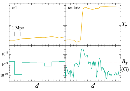
Figure 2: Photon transfer function $T_{\gamma}$ in function of the distance $d$ for a given line of sight (upper panels) and corresponding variations of the extragalactic magnetic field (lower panels). We have taken the photon energy $E=10$ TeV and ALP parameters $m_{a}=2\times 10^{-8}$ eV and $g_{a\gamma}=10^{-11}$ GeV^-1 (HM). Left panels refer to the “cell” model, while right panels represent the more realistic model of our cosmological simulation. In both the cases we have chosen as average value of the magnetic field $\langle B_{T}\rangle=1.6\times 10^{-9}$ G.

Results—We closely follow the technique described in Horns:2012kw ; Mirizzi:2009aj to solve the propagation equations for the photon-ALP ensemble. We document this procedure in the Supplemental Material. In order to account the VHE photon absorption we employ the EBL model of Ref. Franceschini:2008tp as our benchmark. With respect to Horns:2012kw ; Mirizzi:2009aj we also include the refraction effect on VHE photons, recently calculated in Dobrynina:2014qba . This term would be dominated by the energy density of cosmic microwave background photons. It is expected to damp the photon-ALP conversions at $E\gtrsim 1$ TeV Kartavtsev:2016doq . In Fig. 2 we show the photon transfer function $T_{\gamma}$ in a certain range $d$ of its path along a given line of sight (upper panels) in a region in which the extragalactic magnetic field has significant variations (lower panels). We have taken the photon energy $E=10$ TeV. We have chosen as ALP parameters $m_{a}=2\times 10^{-8}$ eV and $g_{a\gamma}=10^{-11}$ GeV^-1, corresponding to the high-mass (HM) square in Fig. 1. Left panels refer to the “cell” model, while right panels represent the model from the cosmological run. The “cell” model has been generated using a fixed (comoving) size of $l_{c}=1.4$ Mpc per cell, which is the typical coherence length of magnetic fields in the newly simulated model, based on spectral analysis. The transverse magnetic field in each cell is chosen as $B_{T}=B_{0}\sin\theta$ where $\theta$ is a random zenithal angle in $[0,\pi)$ and $B_{0}=1.9\times 10^{-9}$ G is the rms of the magnetic field of all realistic realizations. The dashed line in Fig. 2 corresponds to $\langle B_{T}\rangle=\sqrt{2/3}\,B_{0}=1.6\times 10^{-9}$ G which is thus in both cases the ensemble average of the strength of the transverse magnetic field. It can be seen that while in the “cell” model the variations of the $B$ field saturate the maximum value ($B_{0}$), in the more realistic scenario generated by the simulations there are several peaks where $B_{T}\sim 10^{-7}$ G, which are found to correlate with gas structures in the cosmic web (i.e. mostly filaments and outer regions of galaxy clusters and groups). As a consequence, while in the “cell” model $T_{\gamma}$ does not show sizeable variations since the strong mixing regime is suppressed by $m_{a}$ [see Eq. (1)], in the more realistic case one finds a significant jump in $T_{\gamma}$ when the peak in the magnetic field is reached. Indeed, since the conversion probability in ALPs scales as $P_{a\gamma}\sim(g_{a\gamma}B_{T}d)^{2}$, when the strong peak in $B_{T}$ is encountered a strong photon regeneration takes place.

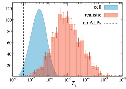
Figure 3: Probability distribution functions for the transfer function $T_{\gamma}$ for photons emitted from a source at redshift $z=0.3$, with $E=10$ TeV and ALPs parameters $m_{a}=2\times 10^{-8}$ eV and $g_{a\gamma}=10^{-11}$ GeV^-1 (HM). Left distribution refers to the cell model, while the right one to the more realistic case. The vertical line corresponds to the no ALPs case.

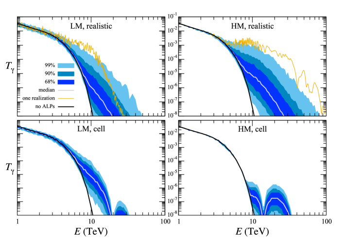
Figure 4: Photon transfer function $T_{\gamma}$ as a function of photon energy for a source at redshift $z=0.3$ for $m_{a}=10^{-10}$ eV and $g_{a\gamma}=4\times 10^{-12}$ GeV^-1 (LM, left panels) and $m_{a}=2\times 10^{-8}$ eV and $g_{a\gamma}=10^{-11}$ GeV^-1 (HM, right panels). The upper panels refer to more realistic models of an extragalactic magnetic field, while lower panels are for the cell model. The black curve corresponds to the case of only absorption onto EBL. The solid grey curve represents the median $T_{\gamma}$ in the presence of ALPs conversions. The orange curve corresponds to conversions for a particular realization of the extragalactic magnetic field. The shaded band is the envelope of the results on all the possible realizations of the extragalactic magnetic field at 68 % (dark blue), 90 % (blue) and 99 % (light blue) C.L., respectively.

Because of the random orientation of the magnetic field, the effect of photon-ALP conversions strongly depends on the orientation of the line of sight. Therefore the photon flux observed at Earth should be better characterized in terms of probability distribution functions, obtained by considering $\gamma\to a$ conversions over different realizations of the extragalactic magnetic field. An example of these distributions is shown in Fig. 3 for a source at redshift $z=0.3$ and energy $E=10$ TeV. We have fixed ALP parameters to the HM case. In the “cell” case, the PDF has been found by simulating $10^{6}$ different realizations of the extragalactic magnetic field. Conversely, in the realistic case, the PDF has been obtained extracting $10^{3}$ onedimensional beams of cells randomly extracted from the outputs of the cosmological simulation at increasing redshift. The $y$ axis shows the number counting for the realistic case only. The vertical thick line corresponds to the no ALPs case. We see that ALP conversions in dynamical magnetic field and in the cell model produce probability distributions which are strongly different. In particular for the cell model the peak in the distribution is $T_{\gamma}\simeq 3\times 10^{-7}$ with a 90 % C.L. in the interval $5.6\times 10^{-8}$–$1.1\times 10^{-6}$, while in the more realistic case one finds the peak at $T_{\gamma}\sim 3\times 10^{-5}$ and a 90 % C.L. in the interval $4.5\times 10^{-7}$–$1.4\times 10^{-4}$. It is evident that a strong enhancement of the transfer function in the more realistic case would imply a significant hardening of the photon spectra with respect to the cell model. Note that in the realistic case the statistical error in each bin is due to the limited number of realizations of the magnetic fields configurations.

In order to discuss the observational signatures in the energy spectra of VHE photon sources we present in Fig. 4 the distribution of photon transfer function $T_{\gamma}$ in function of the photon energy for a source at redshift $z=0.3$ obtained with $10^{3}$ realizations. In the left panels we consider $m_{a}=10^{-10}$ eV and $g_{a\gamma}=4\times 10^{-12}$ GeV^-1, corresponding to the LM case of Fig. 1, while in the right panels we take HM parameters. Upper panels refer to our simulations for magnetic field, while lower ones are for the cell model. The black solid curve represents the $T_{\gamma}$ expected in the presence of only absorption onto EBL. The solid grey curve represents the median $T_{\gamma}$ in the presence of ALPs conversions. The orange curve corresponds to conversions for a particular realization of the extragalactic magnetic field. The shaded band is the envelope of the results on all the possible realizations of the extragalactic magnetic field at 68 % (dark blue), 90 % (blue) and 99 % (light blue) C.L., respectively. According to conventional physics, it turns out that the $T_{\gamma}$ gets dramatically suppressed at high energies ($E\gtrsim 4$ TeV). As expected, including ALP conversions with cell magnetic fields, the enhancement of $T_{\gamma}$ with respect to the standard case is modest since it is suppressed by the small coupling (left panel) or the high ALP mass (right panel). However, when we consider ALP conversions in more realistic magnetic fields the enhancement of $T_{\gamma}$ is striking. ALP conversions in such models would produce a considerable hardening of the spectrum at high enough energies, thereby making it possible to detect VHE photons in a range where no observable signal would be expected according to conventional physics or to conversions with cell magnetic fields. An example of a particular realization is shown by the orange curve. In this specific case we see that the observable photon flux at high energies can be significantly larger than the average one. On this specific line of sight the enhancement of $T_{\gamma}$ with respect to the standard case would reach 3 orders of magnitude. Note also the rapid oscillations observed in the $T_{\gamma}$. These are induced by the the photon dispersion effect on cosmic microwave background Kartavtsev:2016doq (see also Supplemental Material) and would leave observable signatures on the VHE photon spectra unexpected in the standard case. Depending on the particular magnetic realization crossed by the photons, it is also possible to observe a suppression of the photon flux stronger than in the presence of conventional physics. Nevertheless, from Fig. 4 one infers that the cases in which $T_{\gamma}$ is enhanced at high energies are much more probable.

Conclusions—We have studied the conversions of VHE photons into ALPs proposed as a mechanism to reduce the absorption onto EBL, using for the first time more realistic models of extragalactic magnetic fields, obtained from the largest magnetohydrodynamical cosmological simulations in the literature. We find an enhancement of the magnetic field with respect to what was predicted in the naive cell model, due to the fact that simulated magnetic fields display larger fluctuations, correlated with density fluctuations of the cosmic web. This effect would give a significant boost to photon-ALP conversions. Indeed, using more realistic models of the magnetic field we have found significant conversions also in regions of the parameter space consistent with previous astrophysical bounds. This mechanism would produce a significant hardening of the VHE photon spectrum from faraway sources, and we expect such signature to emerge at energies $E\gtrsim 1$ TeV. Therefore, this scenario is testable with the present generation of the Imaging Atmospheric Cherenkov Telescope, covering energies in the range from $\sim$ 50 GeV to $\sim$ 50 TeV Meyer:2014gta ; Consortium:2010bc .

Acknowledgments—We thank Maurizio Giannotti, Manuel Meyer, Georg Raffelt and Pasquale Dario Serpico for reading our manuscript and for useful comments on it. We acknowledge the important collaboration of Claudio Gheller and Marcus Brüggen in the production of the cosmological simulation analyzed in this work. The work of A.M. and D.M. is supported by the Italian Ministero dell’Istruzione, Università e Ricerca (MIUR) and Istituto Nazionale di Fisica Nucleare (INFN) through the “Theoretical Astroparticle Physics” project. F.V. acknowledges the use of computing resources on Piz Daint (ETHZ-CSCS, Lugano) under allocation s585 and s701. F.V. acknowledges financial support from the grant VA 876-3/1 by DFG, and from the European Research Council (ERC) under the European Union’s Horizon 2020 research and innovation program under the Marie-Sklodowska-Curie Grant Agreement No. 664931 and under the “MAGCOW” Starting Grant No. 714196. M.V. is supported by PRIN INAF, PRIN MIUR, INDARK-PD51 and ERC ”cosmoIGM” grants.

Supplemental Material

Setup of photon-ALP oscillations—Photon-ALP mixing occurs in the presence of an external magnetic field ${\bf B}$ due to the interaction term Raffelt:1987im

$${\cal L}_{a\gamma}=-\frac{1}{4}\,g_{a\gamma}F_{\mu\nu}\tilde{F}^{\mu\nu}a=g_{a\gamma}\,{\bf E}\cdot{\bf B}\,a~{},$$ (2)

where $g_{a\gamma}$ is the photon-ALP coupling constant (which has the dimension of an inverse energy).

We consider throughout a monochromatic photon/ALP beam of energy $E$ propagating along the $x_{3}$ direction in a cold ionized and magnetized medium. It has been shown that for very relativistic ALPs and polarized photons, the beam propagation equation can be written in a Schrödinger-like form in which $x_{3}$ takes the role of time Raffelt:1987im ; Kartavtsev:2016doq

$$i\frac{d}{dx_{3}}\left(\begin{array}[]{c}A_{1}(x_{3})\\ A_{2}(x_{3})\\ a(x_{3})\end{array}\right)=\left({\cal H}_{\rm disp}-\frac{i}{2}{\cal H}_{\rm abs}\right)\left(\begin{array}[]{c}A_{1}(x_{3})\\ A_{2}(x_{3})\\ a(x_{3})\end{array}\right)~{},$$ (3)

where $A_{1}(x_{3})$ and $A_{2}(x_{3})$ are the photon linear polarization amplitudes along the $x_{1}$ and $x_{2}$ axis, respectively, $a(x_{3})$ denotes the ALP amplitude. The Hamiltonian ${\cal H}_{\rm disp}$ represents the photon-ALP dispersion matrix, including the mixing and the refractive effects, while ${\cal H}_{\rm abs}$ accounts for the photon absorption effects on the low-energy photon backgrounds. We denote by $T(x_{3},0;E)$ the transfer function, namely the solution of Eq. (3) with initial condition $T(0,0;E)=1$.

The Hamiltonian ${\cal H}_{\rm disp}$ simplifies if we restrict our attention to the case in which ${\bf B}$ is homogeneous. We denote by ${\bf B}_{T}$ the transverse magnetic field, namely its component in the plane normal to the beam direction and we choose the $x_{2}$-axis along ${\bf B}_{T}$ so that $B_{1}$ vanishes. The linear photon polarization state parallel to the transverse field direction ${\bf B}_{T}$ is then denoted by $A_{\parallel}$ and the orthogonal one by $A_{\perp}$. Correspondingly, the mixing matrix can be written as Raffelt:1987im ; Kartavtsev:2016doq

$${\cal H}_{\rm disp}=\left(\begin{array}[]{ccc}\Delta_{\perp}&0&0\\ 0&\Delta_{\parallel}&\Delta_{a\gamma}\\ 0&\Delta_{a\gamma}&\Delta_{a}\end{array}\right)~{},$$ (4)

whose elements are Raffelt:1987im $\Delta_{\perp}\equiv\Delta_{\rm pl}+\Delta_{\perp}^{\rm CM}+\Delta_{\rm CMB},$ $\Delta_{\parallel}\equiv\Delta_{\rm pl}+\Delta_{\parallel}^{\rm CM}+\Delta_{\rm CMB},$ $\Delta_{a\gamma}\equiv{g_{a\gamma}B_{T}}/{2}$ and $\Delta_{a}\equiv-{m_{a}^{2}}/{2E}$, where $m_{a}$ is the ALP mass. The term $\Delta_{\rm pl}\equiv-{\omega^{2}_{\rm pl}}/{2E}$ accounts for plasma effects, where $\omega_{\rm pl}$ is the plasma frequency expressed as a function of the electron density in the medium $n_{e}$ as $\omega_{\rm pl}\simeq 3.69\times 10^{-11}\sqrt{n_{e}/{\rm cm}^{-3}}\,{\rm eV}$. The terms $\Delta_{\parallel,\perp}^{\rm CM}$ describe the Cotton-Mouton effect, i.e. the birefringence of fluids in the presence of a transverse magnetic field. A vacuum Cotton-Mouton effect is expected from QED one-loop corrections to the photon polarization in the presence of an external magnetic field $\Delta_{\mathrm{QED}}=|\Delta_{\perp}^{\rm CM}-\Delta_{\parallel}^{\rm CM}|\propto B^{2}_{T}$, but this effect is completely negligible in the present context. Recently it has been realized that also background photons can contribute to the photon polarization. At this regard a guaranteed contribution is provided by the CMB radiation, leading to $\Delta_{\rm CMB}\propto\rho_{\rm CMB}$ Dobrynina:2014qba . We will show how this term would play a crucial role for the development of the conversions at high energies. An off-diagonal $\Delta_{R}$ would induce the Faraday rotation, which is however totally irrelevant at VHE, and so it has been dropped. For our benchmark values corresponding to the HM point, numerically we find

$$\Delta_{a\gamma} \simeq 1.5\times 10^{-2}\left(\frac{g_{a\gamma}}{10^{-11}\textrm{GeV}^{-1}}\right)\left(\frac{B_{T}}{10^{-9}\,\rm G}\right){\rm Mpc}^{-1}\,,$$

$$\Delta_{a} \simeq -3.2\times 10^{1}\left(\frac{m_{a}}{2\times 10^{-8}{\rm eV}}\right)^{2}\left(\frac{E}{{\rm TeV}}\right)^{-1}{\rm Mpc}^{-1}\,,$$

$$\Delta_{\rm pl} \simeq -1.1\times 10^{-7}\left(\frac{E}{{\rm TeV}}\right)^{-1}\left(\frac{n_{e}}{10^{-3}\,{\rm cm}^{-3}}\right){\rm Mpc}^{-1}\,,$$

$$\Delta_{\rm QED} \simeq 4.1\times 10^{-9}\left(\frac{E}{{\rm TeV}}\right)\left(\frac{B_{T}}{10^{-9}\,\rm G}\right)^{2}{\rm Mpc}^{-1}\,,$$

$$\Delta_{\rm{CMB}} \simeq 0.80\times 10^{-1}\left(\frac{E}{{\rm TeV}}\right){\rm Mpc}^{-1}\,\ .$$ (5)

VHE photons undergo pair production absorption by EBL low energy photons $\gamma_{\rm VHE}\gamma_{\rm EBL}\to e^{+}e^{-}$, dominated by the interactions with optical/infrared EBL photons. The absorptive part of the Hamiltonian can be written in the form

$${\cal H}_{\rm abs}=\left(\begin{array}[]{ccc}\Gamma&0&0\\ 0&\Gamma&0\\ 0&0&0\end{array}\right)~{},$$ (6)

where $\Gamma$ is the photon absorption rate (see Mirizzi:2009aj for details). Several realistic models for the EBL are available in the literature, which are basically in mutual agreement. Among all possible choices, we employ the EBL model Franceschini:2008tp as our benchmark. For crude numerical estimates at zero redshift we use for the absorption rate Mirizzi:2009aj

$$\Gamma=1.1\times 10^{-3}\left(\frac{E}{\rm TeV}\right)^{1.55}{\rm Mpc}^{-1}\,\ .$$ (7)

Single magnetic domain—Considering the propagation of photons in a single magnetic domain with a uniform ${\bf B}$-field with $B_{1}=0$, the component $A_{\perp}$ decouples away, and the propagation equations reduce to a 2-dimensional problem. Its solution follows from the diagonalization of the Hamiltonian through a similarity transformation performed with an orthogonal matrix, parametrized by the (complex) rotation angle $\Theta$ which takes the value Raffelt:1987im ; Kartavtsev:2016doq

$$\Theta=\frac{1}{2}\textrm{arctan}\left(\frac{2\Delta_{a\gamma}}{\Delta_{\parallel}-\Delta_{a}-\frac{i}{2}\Gamma}\right)\,\ .$$ (8)

Note that $\Delta_{a}<0$ and $\Delta_{\parallel}>0$. Therefore, these two contributions always sum and must be separately small to achieve large mixing angle. When $\Delta_{a\gamma}\gg\Delta_{\parallel}-\Delta_{a}$ the photon-ALP mixing is close to maximal, $\Theta\to\pi/4$ (if the absorption is small as well). On the other hand, from Eq. (5) one sees that $\Delta_{\rm CMB}$ grows linearly with the photon energy. Therefore at sufficiently high energies $\Delta_{a\gamma}\ll\Delta_{\parallel}-\Delta_{a}$ and the photon-ALP mixing is suppressed.

One can introduce a generalized (including absorption) photon-ALP oscillations frequency

$$\Delta_{\rm osc}\equiv\left[(\Delta_{\parallel}-\Delta_{a}-\frac{i}{2}\Gamma)^{2}+4\Delta_{a\gamma}^{2}\right]^{1/2}~{}.$$ (9)

In particular, if absorption effect are small the probability for a photon emitted in the state $A_{\parallel}$ to oscillate into an ALP after traveling a distance $d$ is given by Raffelt:1987im

$$P_{\gamma\to a}^{(0)} = {\rm sin}^{2}2\Theta\ {\rm sin}^{2}\left(\frac{\Delta_{\rm osc}\,d}{2}\right)\,\$$ (10)

$$= (\Delta_{a\gamma}d)^{2}\frac{\sin^{2}(\Delta_{\rm osc}d/2)}{(\Delta_{\rm osc}d/2)^{2}}\,\ ,$$

where in the oscillation wave number and mixing angle we set $\Gamma=0$.

From Eq. (5) one would realize that for $E\gtrsim 10$ TeV and $B_{T}\sim 10^{-7}$ G, $\Delta_{a\gamma}\gg\Delta_{a},\Delta_{\rm pl}$. Therefore, neglecting the $\Delta_{\rm CMB}$ refractive term one would obtain $P_{\gamma\to a}^{(0)}\simeq(\Delta_{a\gamma}d)^{2}$, that is energy-independent. However, we see that $\Delta_{\rm CMB}$ is not negligible at these energies and would produce peculiar energy-dependent oscillations imprinting significant features in the VHE photon spectra.

So far, we have been dealing with a beam containing polarized photons, but since at VHE the polarization cannot be measured we better assume that the beam is unpolarized. This is properly done by means of the polarization density matrix

$$\rho(x_{3})=\left(\begin{array}[]{c}A_{1}(x_{3})\\ A_{2}(x_{3})\\ a(x_{3})\end{array}\right)\otimes\left(\begin{array}[]{c}A_{1}(x_{3})\ A_{2}(x_{3})\ a(x_{3})\end{array}\right)^{*}$$ (11)

which obeys the Liouville equation Kartavtsev:2016doq

$$i\frac{d\rho}{dx_{3}}=[{\cal H}_{\rm disp},\rho]-\frac{i}{2}\{{\cal H}_{\rm abs},\rho\}$$ (12)

associated with Eq. (3). Then it follows that the solution of Eq. (12) is given by

$$\rho(x_{3},E)=T(x_{3},0;E)\,\rho(0)\,T^{\dagger}(x_{3},0;E)~{},$$ (13)

where $\rho(0)$ is the initial beam state. Note that for a uniform ${\bf B}$ even if we clearly have

$$T(x_{3},0;E)=e^{-i({\cal H}_{\rm disp}-\frac{i}{2}{\cal H}_{\rm abs})x_{3}}~{}.$$ (14)

Magnetized cosmic web—In the problem discussed in this paper we consider oscillations of VHE photons into ALPs in the extragalactic magnetic fields. Therefore we have to deal with a more general situation than the one depicted in the previous Section. Indeed, as discussed, the extragalactic magnetic field is not constant along the photon line of sight. In the “cell” model the magnetic field can be modeled as a network of a magnetic domains with size set by its coherence length. Although $|{\bf B}|\equiv B_{0}$ is supposed to be the same in every domain, its direction changes randomly from one domain to another. Therefore the propagation over many magnetic domains is clearly a truly 3-dimensional problem, because – due to the randomness of the direction of ${\bf B}$ –the same photon polarization states play the role of either $A_{\parallel}$ and $A_{\perp}$ in different domains. Therefore the Hamiltonian ${\cal H}_{\rm disp}$ entering propagation equation cannot be reduced to a block-diagonal form similar to Eq. (4) in all domains. Rather, we take the $x_{1}$, $x_{2}$, $x_{3}$ coordinate system as fixed once and for all, and – denoting ${\bf b}_{k}$ a random unit vector inside each cell, during their path with a total length $L$ along the line of sight, the beam crosses $n=L/l_{c}$ domains, where $l_{c}$ is the size of each domain: The set $\{{\bf B}_{k}\}_{1\leq k\leq n}=\{B_{0}\,{\bf b}_{k}\}_{1\leq k\leq n}$ represents a given random realization of the beam propagation. Accordingly, in each domain the Hamiltonian ${\cal H}_{\rm disp}$ takes the form Mirizzi:2007hr

$${\cal H}_{\rm disp}^{k}=\left(\begin{array}[]{ccc}\Delta_{xx}&\Delta_{xy}&\Delta_{a\gamma}\,\sin\phi_{k}\\ \Delta_{yx}&\Delta_{yy}&\Delta_{a\gamma}\,\cos\phi_{k}\\ \Delta_{a\gamma}\,\sin\phi_{k}&\Delta_{a\gamma}\,\cos\phi_{k}&\Delta_{a}\\ \end{array}\right)~{},$$ (15)

where $\phi_{k}\in[0,2\pi)$ is the azimuthal (random) angle between the projection of ${\bf b}_{k}$ on the $(x_{1},x_{2})$ plane and the $x_{2}$ axis, and

$$\Delta_{xx}=\Delta_{\parallel}\,\sin^{2}\phi_{k}+\Delta_{\perp}\cos^{2}\phi_{k}~{},$$ (16)

$$\Delta_{xy}=\Delta_{yx}=(\Delta_{\parallel}-\Delta_{\perp})\sin\phi_{k}\,\cos\phi_{k}~{},$$ (17)

$$\Delta_{yy}=\Delta_{\parallel}\cos^{2}\phi_{k}+\Delta_{\perp}\sin^{2}\phi_{k}~{},$$ (18)

while $\Delta_{a\gamma}$ is given by the first of Eqs. (5) with $B_{T}=B_{0}\sin\theta_{k}$, where $\theta_{k}$ is the zenith angle chosen randomly in $\theta_{k}\in[0,\pi)$.

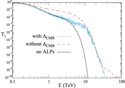
Figure 5: The photon transfer function $T_{\gamma}$ as a function of energy for a source at redshift $z=0.3$ for $m_{a}=10^{-10}$ eV and $g_{a\gamma}=4\times 10^{-12}$ GeV^-1 (LM) for a particular realization with (continuous blue curve) and without (dashed red curve) $\Delta_{\rm CMB}$. The dotted curve corresponds to the case of only absorption onto EBL.

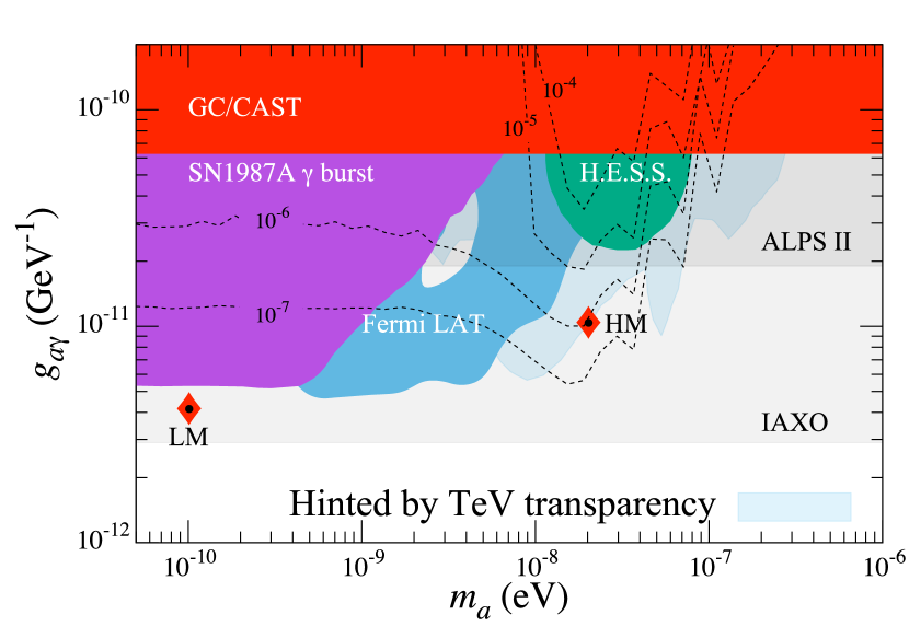
Figure 6: Iso contour lines for transfer function $T_{\gamma}$ for a source at $z=0.3$ and at an energy $E=20$ TeV for cell model (left) and realistic model (right) of $B$-field. Se the text for more details.

Working in terms of the Eq. (12), after the propagation over $n$ magnetic domains the density matrix is given by repeated use of ${\cal H}_{\rm disp}^{k}$, namely

$$\rho_{n}=T({\bf b}_{n},\ldots,{\bf b}_{1})\,\rho_{0}\,T^{\dagger}({\bf b}_{n},\ldots,{\bf b}_{1})~{},$$ (19)

where we have set

$$T({\bf b}_{n},\ldots,{\bf b}_{1})\equiv\prod^{n}_{k=1}T_{k}~{},$$ (20)

with

$$T_{k}=e^{(i{\cal H}_{\rm disp}-\frac{i}{2}{\cal H}_{\rm abs})l_{c}}\,\ ,$$ (21)

which is the transfer function in the $k$-th domain. In a cosmological context however we should remember that $B_{0}$ and $l_{c}$ are no longer fixed but scale as $B_{0}\,(1+z_{k})^{2}$ and $l_{c}/(1+z_{k})$ where $z_{k}$ is the redshift of the cell.

In the realistic case we solve the same equations, but the field ${\bf B}$ is no longer a random vector but its three components are calculated from the numerical model for every realization.

The effect of the $\Delta_{\rm CMB}$ term —We briefly comment on the role of $\Delta_{\rm CMB}$ term on the ALP-photon conversions at high energies. This term due to VHE photon refraction on CMB photons been recently calculated in Dobrynina:2014qba . From Eqs. (9) and (10) it results that assuming $\Delta_{\rm CMB}=0$, when $\Delta_{a\gamma}\gg\Delta_{a},\Delta_{\rm pl}$ $P_{a\gamma}$ would become energy-independent. Conversely, including $\Delta_{\rm CMB}$ this term can mimic a mass term, producing peculiar energy-dependent features. In order to illustrate this effect, in Fig. 5 we show the transfer function $T_{\gamma}$ as a function of energy for a source at redshift $z=0.3$ for $m_{a}=10^{-10}$ eV and $g_{a\gamma}=4\times 10^{-12}$ GeV^-1 (LM case) in presence of ALP oscillations including the $\Delta_{\rm CMB}$ effect (continuous curve) and without it (dashed curve). For comparison it is also shown $T_{\gamma}$ with only absorption on EBL (dotted curve). As predicted $\Delta_{\rm CMB}$ is responsible for the energy-dependent “wiggles” in the $T_{\gamma}(E)$ which are absent when $\Delta_{\rm CMB}=0$. Another important consequence of $\Delta_{\rm CMB}$ is to suppress the transfer function at high energies when $\Delta_{\rm CMB}\gtrsim\Delta_{a\gamma}$ (at $E>30$ TeV in Fig. 5).

Transfer function in the $(g_{a\gamma},m_{a})$ space—In Fig. 6 we show, superposed to the exclusion regions of Fig. 1, curves iso-$T_{\gamma}$ for a source at $z=0.3$ and at energy $E=20$ TeV. Left panel refers to the cell model while right panel is for realistic magnetic field. Each contour corresponds to the 95^th percentile of the distribution of $T_{\gamma}$. In other words, there is a 5% probability that $T_{\gamma}$ is larger than the indicated value. From these curves is evident the enhancement of the area probed with the realistic model at a fixed value of $T_{\gamma}$.

Cosmological Simulations of Extragalactic Magnetic Fields—The simulation used in this work belongs to a dataset of large cosmological simulations produced with the grid-MHD code ENZO Enzo14 , presented in detail Vazza14 and Gheller16 and designed to study the evolution of extragalactic magnetic fields under different physical scenarios. This simulation employed non-radiative physics to evolve a comoving volume of $200^{3}\rm Mpc^{3}$, assuming a cosmology with $H=67.8\rm~{}km/(s\cdot Mpc)$, $\Omega_{b}=0.0478$, $\Omega_{\rm tot}=1.0$, $\Omega_{\Lambda}=0.692$. The magnetic field has been initialized to the uniform value of $B_{0}=1~{}\rm nG$ along each coordinate axis at the begin of the simulation ($z=38$). With its $2400^{3}$ cells/dark matter particles (for the fixed spatial resolution of $83.3$ kpc per cell) this dataset represents the largest magnetohydrodynamical simulation in the literature so far.

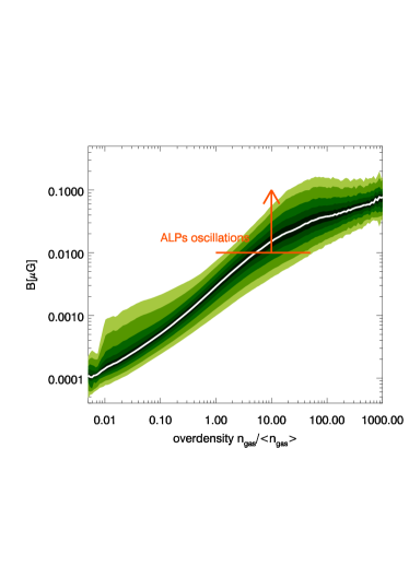
Figure 7: Distribution of typical magnetic field strength as a function of gas overdensity for a representative samples of line of sights through our simulated volume. The different lines mark the percentiles of the distribution at each overdensity, tenfold from 10 to 90%. The additional orange arrow approximately marks the regime in which we observe significant photon-ALPs conversion in the energy range investigated in the paper.

Fig. 7 shows the distribution of magnetic fields as a function of cosmic environment in our simulation. The majority of the investigated volume presents a magnetisztion level that follows the compression/rarefaction of gas: $|{\bf B}|\propto(n_{\rm gas}/\langle n_{\rm gas}\rangle)^{2/3}$, i.e. the frozen-field approximation. The additional scatter on the relation is due structure formation dynamics; in particular the larger fluctuations at the high-density end of the distribution are a product of small-scale dynamo amplification acting within virialized halos.

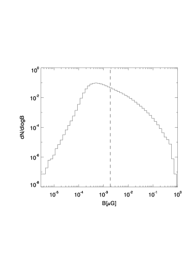
Figure 8: Volume distribution of typical magnetic field strength for the same set of simulated lines of sight as in Fig. 7 (black). The additional dashed line show the r.m.s. magnetic field value for the same distribution.

Fig. 8 gives the volume distribution of magnetic field strength for the same set of lines of sight. The majority of the volume has a magnetization level slightly below the initial seed field (as an effect of adiabatic expansion in voids), yet a pronounced tail with magnetic fields up to $\sim\mu$G is present, largely exceeding the r.m.s. magnetic field measured within the volume, i.e. $1.9\times 10^{-9}\rm G$ (as shown with the vertical grey line). The distribution of extragalactic magnetic fields reproduced in this simulation is a first, important step towards the simulation of possible scenarios for the origin of cosmic magnetic fields, which is presently limited by the constraints from the cosmic microwave background  Planck2015 , and it will also possibly include the magnetization from astrophysical sources, like radio galaxies, starburst winds and jets from active galactic nuclei. The impact of such mechanisms on the conversion of ALPs will be subject of forthcoming work.

References

- (1) J. Jaeckel and A. Ringwald, “The Low-Energy Frontier of Particle Physics,” Ann. Rev. Nucl. Part. Sci. 60, 405 (2010) [arXiv:1002.0329 [hep-ph]].
- (2) G. Raffelt and L. Stodolsky, “Mixing of the photon with low mass particles,” Phys. Rev. D 37, 1237 (1988).
- (3) K. Ehret et al., “New ALPS Results on Hidden-Sector Lightweights,” Phys. Lett. B 689, 149 (2010) [arXiv:1004.1313 [hep-ex]].
- (4) M. Arik et al. [CAST Collaboration], “New solar axion search using the CERN Axion Solar Telescope with 4He filling,” Phys. Rev. D 92, no. 2, 021101 (2015) [arXiv:1503.00610 [hep-ex]].
- (5) L. D. Duffy, P. Sikivie, D. B. Tanner, S. J. Asztalos, C. Hagmann, D. Kinion, L. J. Rosenberg, K. van Bibber, D. B. Yu, and R. F. Bradley,, “A High Resolution Search for Dark-Matter Axions,” Phys. Rev. D 74, 012006 (2006) [astro-ph/0603108].
- (6) P. W. Graham, I. G. Irastorza, S. K. Lamoreaux, A. Lindner and K. A. van Bibber, “Experimental Searches for the Axion and Axion-Like Particles,” Ann. Rev. Nucl. Part. Sci. 65, 485 (2015) [arXiv:1602.00039 [hep-ex]].
- (7) F. Aharonian et al. [H.E.S.S. Collaboration], “A Low level of extragalactic background light as revealed by gamma-rays from blazars,” Nature 440, 1018 (2006) [astro-ph/0508073].
- (8) D. Horns and M. Meyer, “Indications for a pair-production anomaly from the propagation of VHE gamma-rays,” JCAP 1202, 033 (2012) [arXiv:1201.4711 [astro-ph.CO]].
- (9) W. Essey and A. Kusenko, “A new interpretation of the gamma-ray observations of active galactic nuclei,” Astropart. Phys. 33, 81 (2010) [arXiv:0905.1162 [astro-ph.HE]].
- (10) W. Essey, O. E. Kalashev, A. Kusenko and J. F. Beacom, “Secondary photons and neutrinos from cosmic rays produced by distant blazars,” Phys. Rev. Lett. 104, 141102 (2010) [arXiv:0912.3976 [astro-ph.HE]].
- (11) C. Csaki, N. Kaloper, M. Peloso and J. Terning, “Super GZK photons from photon axion mixing,” JCAP 0305, 005 (2003) [hep-ph/0302030].
- (12) A. De Angelis, M. Roncadelli, and O. Mansutti, “Evidence for a new light spin-zero boson from cosmological gamma-ray propagation?,” Phys. Rev. D 76, 121301 (2007) [arXiv:0707.4312 [astro-ph]].
- (13) M. Simet, D. Hooper and P. D. Serpico, “The Milky Way as a Kiloparsec-Scale Axionscope,” Phys. Rev. D 77, 063001 (2008) [arXiv:0712.2825 [astro-ph]].
- (14) A. Dominguez, M. A. Sánchez-Conde and F. Prada, “Axionlike particle imprint in cosmological very-high-energy sources,” JCAP 1111, 020 (2011) [arXiv:1106.1860 [astro-ph.CO]].
- (15) A. De Angelis, G. Galanti and M. Roncadelli, “Relevance of axionlike particles for very-high-energy astrophysics,” Phys. Rev. D 84, 105030 (2011) Erratum: [Phys. Rev. D 87, no. 10, 109903 (2013)] [arXiv:1106.1132 [astro-ph.HE]].
- (16) D. Horns, L. Maccione, M. Meyer, A. Mirizzi, D. Montanino and M. Roncadelli, “Hardening of TeV gamma spectrum of AGNs in galaxy clusters by conversions of photons into axionlike particles,” Phys. Rev. D 86, 075024 (2012) [arXiv:1207.0776 [astro-ph.HE]].
- (17) M. Meyer, D. Horns and M. Raue, “First lower limits on the photon-axionlike particle coupling from very high energy gamma-ray observations,” Phys. Rev. D 87, no. 3, 035027 (2013) [arXiv:1302.1208 [astro-ph.HE]].
- (18) S. Troitsky, “Towards discrimination between galactic and intergalactic axion-photon mixing,” Phys. Rev. D 93, no. 4, 045014 (2016) [arXiv:1507.08640 [astro-ph.HE]].
- (19) A. De Angelis, O. Mansutti and M. Roncadelli, “Axion-Like Particles, Cosmic Magnetic Fields and Gamma-Ray Astrophysics,” Phys. Lett. B 659, 847 (2008) [arXiv:0707.2695 [astro-ph]].
- (20) G. Cantatore, “Satus of the physics program at CAST”. Talk at the Axion Dark Matter Workshop, Stockholm, 5–9 December 2016. Slides available at https://www.nordita.org/docs/agenda/slides-axions2016- cantatore.pdf
- (21) A. Ayala, I. Domìnguez, M. Giannotti, A. Mirizzi and O. Straniero, “Revisiting the bound on axion-photon coupling from Globular Clusters,” Phys. Rev. Lett. 113, no. 19, 191302 (2014) [arXiv:1406.6053 [astro-ph.SR]].
- (22) P. A. R. Ade et al. [Planck Collaboration], “Planck 2015 results. XIX. Constraints on primordial magnetic fields,” Astron. Astrophys. 594, A19 (2016) [arXiv:1502.01594 [astro-ph.CO]].
- (23) P. Blasi, S. Burles and A. V. Olinto, “Cosmological magnetic fields limits in an inhomogeneous universe,” Astrophys. J. 514 (1999) L79 [astro-ph/9812487].
- (24) M. S. Pshirkov, P. G. Tinyakov and F. R. Urban, “New limits on extragalactic magnetic fields from rotation measures,” Phys. Rev. Lett. 116, no. 19, 191302 (2016) [arXiv:1504.06546 [astro-ph.CO]].
- (25) R. Jansson and G. R. Farrar, “A New Model of the Galactic Magnetic Field,” Astrophys. J. 757, 14 (2012) [arXiv:1204.3662 [astro-ph.GA]].
- (26) M. S. Pshirkov, P. G. Tinyakov, P. P. Kronberg and K. J. Newton-McGee, “Deriving global structure of the Galactic Magnetic Field from Faraday Rotation Measures of extragalactic sources,” Astrophys. J. 738, 192 (2011) [arXiv:1103.0814 [astro-ph.GA]].
- (27) N. Oppermann et al., “An improved map of the Galactic Faraday sky,” Astron. Astrophys. 542, A93 (2012) [arXiv:1111.6186 [astro-ph.GA]].
- (28) S. A. Mao, B. M. Gaensler, M. Haverkorn, E. G. Zweibel, G. J. Madsen, N. M. McClure-Griffiths, A. Shukurov and P. P. Kronberg, “A Survey of Extragalactic Faraday Rotation at High Galactic Latitude: The Vertical Magnetic Field of the Milky Way towards the Galactic Poles,” Astrophys. J. 714, 1170 (2010) [arXiv:1003.4519 [astro-ph.GA]].
- (29) A. Payez, C. Evoli, T. Fischer, M. Giannotti, A. Mirizzi and A. Ringwald, “Revisiting the SN1987A gamma-ray limit on ultralight axionlike particles,” JCAP 1502, no. 02, 006 (2015) [arXiv:1410.3747 [astro-ph.HE]].
- (30) M. Ajello et al. [Fermi-LAT Collaboration], “Search for Spectral Irregularities due to Photon?Axionlike-Particle Oscillations with the Fermi Large Area Telescope,” Phys. Rev. Lett. 116, no. 16, 161101 (2016) [arXiv:1603.06978 [astro-ph.HE]].
- (31) M. Berg, J. P. Conlon, F. Day, N. Jennings, S. Krippendorf, A. J. Powell and M. Rummel, “Searches for Axion-Like Particles with NGC1275: Observation of Spectral Modulations,” arXiv:1605.01043 [astro-ph.HE].
- (32) J. P. Conlon, F. Day, N. Jennings, S. Krippendorf and M. Rummel, “Constraints on Axion-Like Particles from Non-Observation of Spectral Modulations for X-ray Point Sources,” arXiv:1704.05256 [astro-ph.HE].
- (33) A. Abramowski et al. [H.E.S.S. Collaboration], “Constraints on axionlike particles with H.E.S.S. from the irregularity of the PKS 2155-304 energy spectrum,” Phys. Rev. D 88, no. 10, 102003 (2013) [arXiv:1311.3148 [astro-ph.HE]].
- (34) S. Angus, J. P. Conlon, M. C. D. Marsh, A. J. Powell and L. T. Witkowski, “Soft X-ray Excess in the Coma Cluster from a Cosmic Axion Background,” JCAP 1409, no. 09, 026 (2014) doi:10.1088/1475-7516/2014/09/026 [arXiv:1312.3947 [astro-ph.HE]].
- (35) C. Wang and D. Lai, “Axion-photon Propagation in Magnetized Universe,” JCAP 1606, no. 06, 006 (2016) [arXiv:1511.03380 [astro-ph.HE]].
- (36) A. Kartavtsev, G. Raffelt and H. Vogel, “Extragalactic photon-ALP conversion at CTA energies,” JCAP 1701, 024 (2017) [arXiv:1611.04526 [astro-ph.HE]].
- (37) E. Masaki, A. Aoki and J. Soda, “Photon-Axion Conversion, Magnetic Field Configuration and Polarization of Photons,” arXiv:1702.08843 [astro-ph.CO].
- (38) F. Vazza, M. Brüggen, C. Gheller and P. Wang, “On the amplification of magnetic fields in cosmic filaments and galaxy clusters,” Mon. Not. Roy. Astron. Soc. 445, no. 4, 3706 (2014) [arXiv:1409.2640 [astro-ph.CO]].
- (39) C. Gheller, F. Vazza, M. Brüggen, M. Alpaslan, B. W. Holwerda, A. Hopkins and J. Liske, “Evolution of cosmic filaments and of their galaxy population from MHD cosmological simulations,” Mon. Not. Roy. Astron. Soc. 462, no. 1, 448 (2016) [arXiv:1607.01406 [astro-ph.CO]].
- (40) A. Mirizzi, G. G. Raffelt and P. D. Serpico, “Photon-axion conversion as a mechanism for supernova dimming: Limits from CMB spectral distortion,” Phys. Rev. D 72, 023501 (2005) [astro-ph/0506078].
- (41) I. G. Irastorza et al., “Towards a new generation axion helioscope,” JCAP 1106, 013 (2011) [arXiv:1103.5334 [hep-ex]].
- (42) M. Meyer, M. Giannotti, A. Mirizzi, J. Conrad and M. A. Sánchez-Conde, “Fermi Large Area Telescope as a Galactic Supernovae Axionscope,” Phys. Rev. Lett. 118, no. 1, 011103 (2017) [arXiv:1609.02350 [astro-ph.HE]].
- (43) G. L. Bryan et al. [ENZO Collaboration], “Enzo: An Adaptive Mesh Refinement Code for Astrophysics,” Astrophys. J. Suppl. 211, 19 (2014) [arXiv:1307.2265 [astro-ph.IM]].
- (44) P. Wang, T. Abel and R. Kaehler, “Adaptive Mesh Fluid Simulations on GPU,” New Astron. 15, 581 (2010) [arXiv:0910.5547 [astro-ph.CO]].
- (45) A. Mirizzi and D. Montanino, “Stochastic conversions of TeV photons into axionlike particles in extragalactic magnetic fields,” JCAP 0912 (2009) 004 [arXiv:0911.0015 [astro-ph.HE]].
- (46) A. Franceschini, G. Rodighiero and M. Vaccari, “The extragalactic optical-infrared background radiations, their time evolution and the cosmic photon-photon opacity,” Astron. Astrophys. 487, 837 (2008) [arXiv:0805.1841 [astro-ph]].
- (47) A. Dobrynina, A. Kartavtsev and G. Raffelt, “Photon-photon dispersion of TeV gamma rays and its role for photon-ALP conversion,” Phys. Rev. D 91, 083003 (2015) [arXiv:1412.4777 [astro-ph.HE]].
- (48) M. Meyer and J. Conrad, “Sensitivity of the Cherenkov Telescope Array to the detection of axionlike particles at high gamma-ray opacities,” JCAP 1412, no. 12, 016 (2014) [arXiv:1410.1556 [astro-ph.HE]].
- (49) M. Actis et al. [CTA Consortium], “Design concepts for the Cherenkov Telescope Array CTA: An advanced facility for ground-based high-energy gamma-ray astronomy,” Exper. Astron. 32, 193 (2011) [arXiv:1008.3703 [astro-ph.IM]].
- (50) A. Mirizzi, G. G. Raffelt and P. D. Serpico, “Signatures of axionlike particles in the spectra of TeV gamma-ray sources,” Phys. Rev. D 76 (2007) 023001 [arXiv:0704.3044 [astro-ph]].