Generalized negative binomial distributions as mixed geometric laws and related limit theorems

Abstract. In this paper we study a wide and flexible family of discrete distributions, the so-called generalized negative binomial (GNB) distributions that are mixed Poisson distributions in which the mixing laws belong to the class of generalized gamma (GG) distributions. The latter was introduced by E. W. Stacy as a special family of lifetime distributions containing gamma, exponential power and Weibull distributions. These distributions seem to be very promising in the statistical description of many real phenomena being very convenient and almost universal models for the description of statistical regularities in discrete data. Analytic properties of GNB distributions are studied. A GG distribution is proved to be a mixed exponential distribution if and only if the shape and exponent power parameters are no greater than one. The mixing distribution is written out explicitly as a scale mixture of strictly stable laws concentrated on the nonnegative halfline. As a corollary, the representation is obtained for the GNB distribution as a mixed geometric distribution. The corresponding scheme of Bernoulli trials with random probability of success is considered. Within this scheme, a random analog of the Poisson theorem is proved establishing the convergence of mixed binomial distributions to mixed Poisson laws. Limit theorems are proved for random sums of independent random variables in which the number of summands has the GNB distribution and the summands have both light- and heavy-tailed distributions. The class of limit laws is wide enough and includes the so-called generalized variance gamma distributions. Various representations for the limit laws are obtained in terms of mixtures of Mittag-Leffler, Linnik or Laplace distributions. Limit theorems are proved establishing the convergence of the distributions of statistics constructed from samples with random sizes obeying the GNB distribution to generalized variance gamma distributions. Some applications of GNB distributions in meteorology are discussed.

Key words: generalized gamma distribution, Weibull distribution, mixed exponential distribution, mixed Poisson distribution, negative binomial distribution, mixed geometric distribution, Bernoulli trials, mixed binomial distribution, random Poisson theorem, strictly stable distribution, Rényi theorem, Mittag-Leffler distribution, Linnik distribution, Laplace distribution, normal mixture, random sum, random sample size

1 Introduction

1.1 Motivation

In this paper we study a wide and flexible family of discrete distributions, the so-called generalized negative binomial (GNB) distributions that are mixed Poisson distributions in which the mixing laws belong to the class of generalized gamma distributions. These distributions seem to be very promising in the statistical description of many real phenomena being very convenient and almost universal models.

It is necessary to explain why we consider this combination of the mixed and mixing distributions. First of all, the Poisson mixing kernel is used for the following reasons. Pure Poisson processes can be regarded as best models of stationary (time-homogeneous) chaotic flows of events [1]. Recall that the attractiveness of a Poisson process as a model of homogeneous discrete stochastic chaos is due to at least two reasons. First, Poisson processes are point processes characterized by that time intervals between successive points are independent random variables with one and the same exponential distribution and, as is well known, the exponential distribution possesses the maximum differential entropy among all absolutely continuous distributions concentrated on the nonnegative half-line with finite expectations, whereas the entropy is a natural and convenient measure of uncertainty. Second, the points forming the Poisson process are uniformly distributed along the time axis in the sense that for any finite time interval $[t_{1},t_{2}]$, $t_{1}<t_{2}$, the conditional joint distribution of the points of the Poisson process which fall into the interval $[t_{1},t_{2}]$ under the condition that the number of such points is fixed and equals, say, $n$, coincides with the joint distribution of the order statistics constructed from an independent sample of size $n$ from the uniform distribution on $[t_{1},t_{2}]$ whereas the uniform distribution possesses the maximum differential entropy among all absolutely continuous distributions concentrated on finite intervals and very well corresponds to the conventional impression of an absolutely unpredictable random variable (r.v.) (see, e. g., [9, 1]). But in actual practice, as a rule, the parameters of the chaotic stochastic processes are influenced by poorly predictable ‘‘extrinsic’’ factors which can be regarded as stochastic so that most reasonable probabilistic models of non-stationary (time-non-homogeneous) chaotic point processes are doubly stochastic Poisson processes also called Cox processes (see, e. g., [15, 16, 1]). These processes are defined as Poisson processes with stochastic intensities. Such processes proved to be adequate models in insurance [15, 16, 1], financial mathematics [27], physics [25] and many other fields. Their one-dimensional distributions are mixed Poisson.

In order to have a flexible model of a mixing distribution which is ‘‘responsible’’ for the description of statistical regularities of the manifestation of ‘‘outer’’ stochastic factors we suggest to use the generalized gamma $($GG$)$ distributions defined by the density

$$g^{*}(x;r,\alpha,\lambda)=\frac{|\alpha|\lambda^{r}}{\Gamma(r)}x^{\alpha r-1}e^{-\lambda x^{\alpha}},\ \ \ \ x\geq 0,$$

with $\alpha\in\mathbb{R}$, $\lambda>0$, $r>0$. The class of GG distributions was first described as a unitary family in 1962 by E. Stacy [50] as the class of probability distributions simultaneously containing both Weibull and gamma distributions. The family of GG distributions contains practically all the most popular absolutely continuous distributions concentrated on the non-negative half-line. In particular, the family of GG distributions contains:

• the gamma distribution $(\alpha=1)$ and its special cases –

  • the exponential distribution ($\alpha=1$, $r=1$),

  • the Erlang distribution ($\alpha=1$, $r\in\mathbb{N}$),

  • the chi-square distribution ($\alpha=1$, $\lambda=\frac{1}{2}$);

• the Nakagami distribution ($\alpha=2$);

• the half-normal (folded normal) distribution (the distribution of the maximum of a standard Wiener process on the interval $[0,1]$) ($\alpha=2$, $r=\frac{1}{2}$);

• the Rayleigh distribution ($\alpha=2$, $r=1$);

• the chi-distribution ($\alpha=2$, $\lambda=1/\sqrt{2}$);

• the Maxwell distribution (the distribution of the absolute values of the velocities of moleculas in a dilute gas) ($\alpha=2$, $r=\frac{3}{2}$);

• the Weibull–Gnedenko distribution (the extreme value distribution of type III) ($r=1$, $\alpha>0$);

• the (folded) exponential power distribution ($\alpha>0$, $r=\frac{1}{\alpha}$);

• the inverse gamma distribution ($\alpha=-1$) and its special case –

  • the Lévy distribution (the one-sided stable distribution with the characteristic exponent $\frac{1}{2}$ – the distribution of the first hit time of the unit level by the Brownian motion) ($\alpha=-1$, $r=\frac{1}{2}$);

• the Fréchet distribution (the extreme value distribution of type II) ($r=1$, $\alpha<0$)

and other laws. The limit point of the class of GG distributions is

• the log-normal distribution ($r\to\infty$).

GG distributions are widely applied in many practical problems, first of all, related to image or signal processing. There are dozens of papers dealing with the application of GG distributions as models of regularities observed in practice. Apparently, the popularity of GG distributions is due to that most of them can serve as adequate asymptotic approximations, since all the representatives of the class of GG distributions listed above appear as limit laws in various limit theorems of probability theory in rather simple limit schemes. Below we will formulate a general limit theorem (an analog of the law of large numbers) for random sums of independent r.v.’s in which the GG distributions are limit laws.

Our interest to these distribution was directly motivated by the problem of modeling some statistical regularities in precipitation. In most papers dealing with the statistical analysis of meteorological data available to the authors, the suggested analytical models for the observed statistical regularities in precipitation are rather ideal and far from being adequate. For example, it is traditionally assumed that the duration of a wet period (the number of subsequent wet days) follows the geometric distribution (for example, see [56]) despite that the goodness-of-fit of this model is very far from being admissible. Perhaps, this prejudice is based on the conventional interpretation of the geometric distribution in terms of the Bernoulli trials as the distribution of the number of subsequent wet days (‘‘successes’’) till the first dry day (‘‘failure’’). But the framework of Bernoulli trials assumes that the trials are independent whereas a thorough statistical analysis of precipitation data registered at different points demonstrates that the sequence of dry and wet days is not only devoid of the independence property, but is also not Markovian, so that the framework of Bernoulli trials is absolutely inadequate for analyzing meteorological data.

It turned out that the statistical regularities of the number of subsequent wet days can be very reliably modeled by the negative binomial distribution with the shape parameter less than one. For example, in [34] the data registered in so climatically different points as Potsdam (Brandenburg, Germany) and Elista (Kalmykia, Russia) was analyzed and it was demonstrated that the fluctuations of the numbers of successive wet days with very high confidence fit the negative binomial distribution with shape parameter $r\approx 0.85$. In the same paper a schematic attempt was undertaken to explain this phenomenon by the fact that negative binomial distributions can be represented as mixed Poisson laws with mixing gamma-distributions whereas the Poisson distribution is the best model for the discrete stochastic chaos (see, e. g., [19, 26]) and the mixing distribution accumulates the stochastic influence of factors that can be assumed exogenous with respect to the local system under consideration.

Negative binomial distributions are special cases of generalized negative binomial (GNB) distributions which are mixed Poisson distributions with mixing conducted with respect to a GG distribution. This family of discrete distributions is very wide and embraces Poisson distributions (as limit points corresponding to a degenerate mixing distribution), negative binomial (Polya) distributions including geometric distributions (corresponding to the gamma mixing distribution, see [17]), Sichel distributions (corresponding to the inverse gamma mixing distributions, see [49]), Weibull–Poisson distributions (corresponding to the Weibull mixing distributions, see [30]) and many other types supplying descriptive statistics with many flexible models. More examples of mixed Poisson laws can be found in [16, 51].

It is quite natural to expect that, having introduced one more free parameter into the pure negative binomial model, namely, the power parameter in the exponent of the original gamma mixing distribution, instead of the negative binomial model one might obtain a more flexible GNB model that provides even better fit with the statistical data of the durations of wet days. The analysis of the real data shows that this is indeed so. On Fig. 1 there are the histogram constructed from real data of 3320 wet periods in Potsdam and the fitted negative binomial distribution (that is, the mixed Poisson distribution with the GG mixing law with $\alpha=1$) (right) and the fitted GNB distribution with $\alpha=0.917$ (left). The $L_{1}$-distance between the histogram and the fitted GNB distribution is 0.02637 that is nearly 1.26 times less than the $L_{1}$-distance between the histogram and the fitted negative binomial model (equal to 0.03318).

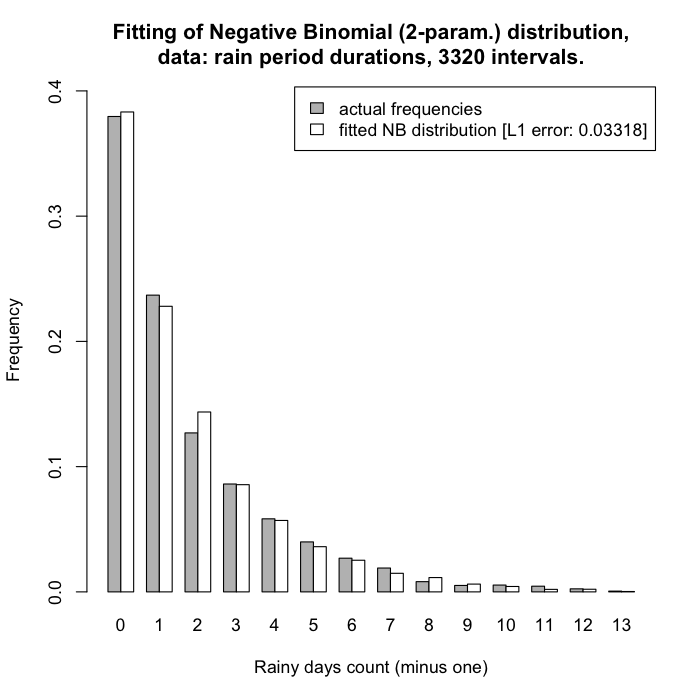
(a)

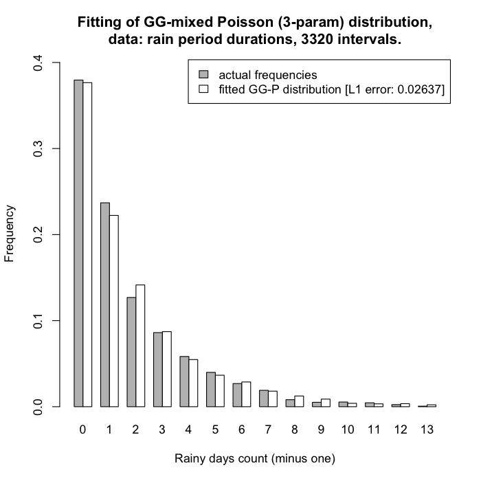
(b)

Fig. 1: The histogram constructed from real data of 3320 wet periods in Potsdam and the fitted negative binomial distribution (a) and the fitted GG-mixed Poisson distribution with $\alpha=0.917$ (b).

The purpose of the present paper is two-fold. First, we try to give further theoretic explanation of the high adequacy of the negative binomial model for the description of meteorological data. For this purpose we use the concept of a mixed geometric law introduced in [29] (also see [30, 31]). Having first proved that any GG distribution with shape parameter $r$ and exponent power parameter $\gamma$ less than one is mixed exponential and thus generalizing Gleser’s similar theorem on gamma-distributions [8], we then prove that any mixed Poisson distribution with the generalized gamma mixing law (GNB distribution) with shape parameter and exponent power parameter less than one is actually mixed geometric. GG distributions with exponent power less than one are of special interest since they occupy an intermediate position between distributions with exponentially decreasing tails (e. g., exponential and gamma-distributions) and heavy-tailed distributions with Zipf–Pareto power-type decrease of tails.

The mixed geometric distribution can be interpreted in terms of the Bernoulli trials as follows. First, as a result of some <<preliminary>> experiment the value of some random variable taking values in $[0,1]$ is determined which is then used as the probability of success in the sequence of Bernoulli trials in which the original <<unconditional>> mixed Poisson random variable is nothing else than the <<conditionally>> geometrically distributed random variable having the sense of the number of trials up to the first failure. This makes it possible to assume that the sequence of wet/dry days is not independent, but is conditionally independent and the random probability of success is determined by some outer stochastic factors. As such, we can consider the seasonality or the type of the cause of a rainy period. So, since the GG distribution is a more general and hence, more flexible model than the ‘‘pure’’ gamma-distribution, there arises a hope that the GNB distribution could provide even better goodness of fit to the statistical regularities in the duration of wet periods than the ‘‘pure’’ negative binomial distribution.

Second, we study analytic and asymptotic properties of probability models closely related to GNB distributions such as the distributions of statistics constructed from samples with random sizes having the GNB distribution. The obtained results can serve as a theoretical explanation of some mixed models used in the statistical analysis.

1.2 Notation and definitions

In the paper, conventional notation is used. The symbols $\stackrel{{\scriptstyle d}}{{=}}$ and $\Longrightarrow$ denote the coincidence of distributions and convergence in distribution, respectively.

In what follows, for brevity and convenience, the results will be presented in terms of r.v.’s with the corresponding distributions. It will be assumed that all the r.v.’s are defined on the same probability space $(\Omega,\,\mathfrak{F},\,{\sf P})$.

A r.v. having the gamma distribution with shape parameter $r>0$ and scale parameter $\lambda>0$ will be denoted $G_{r,\lambda}$,

$${\sf P}(G_{r,\lambda}<x)=\int_{0}^{x}g(z;r,\lambda)dz,\ \ \text{with}\ \ g(x;r,\lambda)=\frac{\lambda^{r}}{\Gamma(r)}x^{r-1}e^{-\lambda x},\ x\geq 0,$$

where $\Gamma(r)$ is Euler’s gamma-function, $\Gamma(r)=\int_{0}^{\infty}x^{r-1}e^{-x}dx$, $r>0$.

In this notation, obviously, $G_{1,1}$ is a r.v. with the standard exponential distribution: ${\sf P}(G_{1,1}<x)=\big{[}1-e^{-x}\big{]}{\bf 1}(x\geq 0)$ (here and in what follows ${\bf 1}(A)$ is the indicator function of a set $A$).

The gamma distribution is a particular representative of the class of generalized gamma distributions (GG distributions), which were first described in [50] as a special family of lifetime distributions containing both gamma and Weibull distributions.

Definition 1. A generalized gamma $($GG$)$ distribution is the absolutely continuous distribution defined by the density

$$g^{*}(x;r,\alpha,\lambda)=\frac{|\alpha|\lambda^{r}}{\Gamma(r)}x^{\alpha r-1}e^{-\lambda x^{\alpha}},\ \ \ \ x\geq 0,$$

with $\alpha\in\mathbb{R}$, $\lambda>0$, $r>0$.

The properties of GG distributions are described in [50, 55]. A r.v. with the density $g^{*}(x;r,\alpha,\lambda)$ will be denoted $G^{*}_{r,\alpha,\lambda}$.

For a r.v. with the Weibull distribution, a particular case of GG distributions corresponding to the density $g^{*}(x;1,\alpha,1)$ and the distribution function (d.f.) $\big{[}1-e^{-x^{\alpha}}\big{]}{\bf 1}(x\geq 0)$ with $\alpha>0$, we will use a special notation $W_{\alpha}$. Thus, $G_{1,1}\stackrel{{\scriptstyle d}}{{=}}W_{1}$. The density $g^{*}(x;1,\alpha,1)$ with $\alpha<0$ defines the Fréchet or inverse Weibull distribution. It is easy to see that $W_{1}^{1/\alpha}\stackrel{{\scriptstyle d}}{{=}}W_{\alpha}$.

In what follows we will be mostly interested in GG distributions with $\alpha\in(0,1]$.

A r.v. with the standard normal d.f. $\Phi(x)$ will be denoted $X$,

$${\sf P}(X<x)=\Phi(x)=\frac{1}{\sqrt{2\pi}}\int_{-\infty}^{x}e^{-z^{2}/2}dz,\ \ \ \ x\in\mathbb{R}.$$

The d.f. and the density of a strictly stable distribution with the characteristic exponent $\alpha$ and shape parameter $\theta$ defined by the characteristic function (ch.f.)

$$\mathfrak{f}(t;\alpha,\theta)=\exp\big{\{}-|t|^{\alpha}\exp\{-{\textstyle\frac{1}{2}}i\pi\theta\alpha\mathrm{sign}t\}\big{\}},\ \ \ \ t\in\mathbb{R},$$

where $0<\alpha\leq 2$, $|\theta|\leq\min\{1,\frac{2}{\alpha}-1\}$, will be respectively denoted $F(x;\alpha,\theta)$ and $f(x;\alpha,\theta)$ (see, e. g., [57]). A r.v. with the d.f. $F(x;\alpha,\theta)$ will be denoted $S_{\alpha,\theta}$. To symmetric strictly stable distributions there correspond the value $\theta=0$ and the ch.f. $\mathfrak{f}(t;\alpha,0)=e^{-|t|^{\alpha}}$, $t\in\mathbb{R}$. Hence, it is easy to see that $S_{2,0}\stackrel{{\scriptstyle d}}{{=}}\sqrt{2}X$.

To one-sided strictly stable distributions concentrated on the nonnegative halfline there correspond the values $\theta=1$ and $0<\alpha\leq 1$. The pairs $\alpha=1$, $\theta=\pm 1$ correspond to the distributions degenerate in $\pm 1$, respectively. All the other strictly stable distributions are absolutely continuous. Stable densities cannot explicitly be represented via elementary functions with four exceptions: the normal distribution ($\alpha=2$, $\theta=0$), the Cauchy distribution ($\alpha=1$, $\theta=0$), the Lévy distribution ($\alpha=\frac{1}{2}$, $\theta=1$) and the distribution symmetric to the Lévy law ($\alpha=\frac{1}{2}$, $\theta=-1$). Expressions of stable densities in terms of the Fox functions (generalized Meijer G-functions) can be found in [47, 53].

According to the <<multiplication theorem>> (see, e. g., theorem 3.3.1 in [57]) for any admissible pair of parameters $(\alpha,\,\theta)$ and any $\alpha^{\prime}\in(0,1]$ the multiplicative representation $S_{\alpha\alpha^{\prime},\theta}\stackrel{{\scriptstyle d}}{{=}}S_{\alpha,\theta}\cdot S_{\alpha^{\prime},1}^{1/\alpha}$ holds, in which the factors on the right-hand side are independent. In particular, for any $\alpha\in(0,2]$

$$S_{\alpha,0}\stackrel{{\scriptstyle d}}{{=}}X\sqrt{2S_{\alpha/2,1}},$$

that is, any symmetric strictly stable distribution is a normal scale mixture.

It is well known that if $0<\alpha<2$, then ${\sf E}|S_{\alpha,\theta}|^{\beta}<\infty$ for any $\beta\in(0,\alpha)$, but the moments of the r.v. $S_{\alpha,\theta}$ of orders $\beta\geq\alpha$ do not exist (see, e. g., [57]). Despite the absence of explicit expressions for the densities of stable distributions in terms of elementary functions, it can be shown [28] that

$${\sf E}|S_{\alpha,0}|^{\beta}=\frac{2^{\beta}}{\sqrt{\pi}}\cdot\frac{\Gamma\big{(}\frac{\beta+1}{2}\big{)}\Gamma\big{(}\frac{\alpha-\beta}{\alpha}\big{)}}{\Gamma\big{(}\frac{2-\beta}{\beta}\big{)}}$$

for $0<\beta<\alpha<2$ and

$${\sf E}S_{\alpha,1}^{\beta}=\frac{\Gamma\big{(}1-\frac{\beta}{\alpha}\big{)}}{\Gamma(1-\beta)}$$

for $0<\beta<\alpha\leq 1$.

In [39, 33, 32] it was proved that if $\alpha\in(0,1)$ and the i.i.d. r.v.’s $S_{\alpha,1}$ and $S^{\prime}_{\alpha,1}$ have the same strictly stable distribution, then the density $v_{\alpha}(x)$ of the r.v. $R_{\alpha}=S_{\alpha,1}/S^{\prime}_{\alpha,1}$ has the form

$$v_{\alpha}(x)=\frac{\sin(\pi\alpha)x^{\alpha-1}}{\pi[1+x^{2\alpha}+2x^{\alpha}\cos(\pi\alpha)]},\ \ \ x>0.$$

The distribution of a r.v. $Z$ is said to belong to the domain of normal attraction of the strictly stable law $F(x;\alpha,\theta)$, $\mathcal{L}(Z)\in DNA\big{(}F(x;\alpha,\theta)\big{)}$, if there exists a finite positive constant $c$ such that

$$\frac{c}{n^{1/\alpha}}\sum\nolimits_{j=1}^{n}Z_{j}\Longrightarrow S_{\alpha,\theta}\ \ \ (n\to\infty),$$

where $Z_{1},Z_{2},...$ are independent copies of the r.v. $Z$. In what follows we will consider the standard scale case and let $c=1$. In [52] it was shown that if $\mathcal{L}(Z)\in DNA\big{(}F(x;\alpha,\theta)\big{)}$, then ${\sf E}|Z|^{\beta}=\infty$ for any $\beta>\alpha$.

A r.v. $N_{r,p}$ is said to have the negative binomial distribution with parameters $r>0$ and $p\in(0,1)$, if

$${\sf P}(N_{r,p}=k)=\frac{\Gamma(r+k)}{k!\Gamma(r)}\cdot p^{r}(1-p)^{k},\ \ \ \ k=0,1,2,...$$

A particular case of the negative binomial distribution corresponding to the value $r=1$ is the geometric distribution. Let $p\in(0,1)$ and let $N_{1,p}$ be the r.v. having the geometric distribution with parameter $p\,$:

$${\sf P}(N_{1,p}=k)=p(1-p)^{k},\ \ \ \ k=0,1,2,...$$

This means that for any $m\in\mathbb{N}$

$${\sf P}(N_{1,p}\geq m)=\sum\nolimits_{k=m}^{\infty}p(1-p)^{k}=(1-p)^{m}.$$

Definition 2. Let $Y$ be a r.v. taking values in the interval $(0,1)$. Moreover, let for all $p\in(0,1)$ the r.v. $Y$ and the geometrically distributed r.v. $N_{1,p}$ be independent. Let $V=N_{1,Y}$, that is, $V(\omega)=N_{1,Y(\omega)}(\omega)$ for any $\omega\in\Omega$. The distribution

$${\sf P}(V\geq m)=\int_{0}^{1}(1-y)^{m}d{\sf P}(Y<y),\ \ \ m\in\mathbb{N},$$

of the r.v. $V$ will be called $Y$-mixed geometric [29].

Let $\alpha\in(0,1]$. The distribution with the Laplace–Stieltjes transform (L.–S.t.)

$$\mathfrak{m}(s;\alpha)=\frac{1}{1+s^{\alpha}},\ \ \ s\geq 0.$$

is conventionally called the Mittag-Leffler distribution. The origin of this term is due to the form of the probability density

$$f^{M}(x;\alpha)=\frac{1}{x^{1-\alpha}}\sum\nolimits_{n=0}^{\infty}\frac{(-1)^{n}x^{\alpha n}}{\Gamma(\alpha n+1)}=-\frac{d}{dx}E_{\alpha}(-x^{\alpha}),\ \ \ x\geq 0,$$

corresponding to L.–S.t. (4), where $E_{\alpha}(z)$ is the Mittag-Leffler function with index $\alpha$ that is defined as the power series

$$E_{\alpha}(z)=\sum\nolimits_{n=0}^{\infty}\frac{z^{n}}{\Gamma(\alpha n+1)},\ \ \ \alpha>0,\ z\in\mathbb{Z}.$$

The distribution function corresponding to density (5) will be denoted $F^{M}(x;\alpha)$. The r.v. with the d.f. $F^{M}(x;\alpha)$ will be denoted $M_{\alpha}$. In [32] the integral representation

$$f^{M}(x;\alpha)=\frac{\sin(\pi\alpha)}{\pi}\int_{0}^{\infty}\frac{z^{\alpha}e^{-zx}dz}{1+z^{2\alpha}+2z^{\alpha}\cos(\pi\alpha)},\ \ \ x>0,$$

for the Mittag-Leffler density was proved.

With $\alpha=1$, the Mittag-Leffler distribution turns into the standard exponential distribution, that is, $M_{1}\stackrel{{\scriptstyle d}}{{=}}W_{1}$. But with $\alpha<1$ the Mittag-Leffler distribution density has a heavy power-type tail: from the well-known asymptotic properties of the Mittag-Leffler function it can be deduced that if $0<\alpha<1$, then

$$f^{M}(x;\alpha)\sim\frac{\sin(\alpha\pi)\Gamma(\alpha+1)}{\pi x^{\alpha+1}}$$

as $x\to\infty$, see, e. g., [14].

It is well-known that the Mittag-Leffler distribution is stable with respect to geometric summation (or geometrically stable). This means that if $X_{1},X_{2},...$ are independent random variables and $N_{1,p}$ is the random variable independent of $X_{1},X_{2},...$ and having the geometric distribution (3), then for each $p\in(0,1)$ there exists a constant $a_{p}>0$ such that $a_{p}\big{(}X_{1}+...+X_{N_{1,p}}\big{)}\Longrightarrow M_{\alpha}$ as $p\to 0$, see, e. g., [5] or [20]. Moreover, as long ago as in 1965 it was shown by I. Kovalenko [40] that the distributions with L.–S.t:s (4) are the only possible limit laws for the distributions of appropriately normalized geometric sums of the form $a_{p}\big{(}X_{1}+...+X_{N_{1,p}}\big{)}$ as $p\to 0$, where $X_{1},X_{2},...$ are independent identically distributed nonnegative random variables and $N_{1,p}$ is the random variable with geometric distribution (3) independent of the sequence $X_{1},X_{2},...$ for each $p\in(0,1)$. The proofs of this result were reproduced in [10, 11] and [9]. In these books the class of distributions with Laplace transforms (4) was not identified as the class of Mittag-Leffler distributions but was called class $\mathcal{K}$ after I. Kovalenko.

Twenty five years later this limit property of the Mittag-Leffler distributions was re-discovered by A. Pillai in [45, 46] who proposed the term Mittag-Leffler distribution for the distribution with Laplace transform (1). Perhaps, since the works [40, 10, 11] were not easily available to probabilists, the term class $\mathcal{K}$ distribution did not take roots in the literature whereas the term Mittag-Leffler distribution became conventional.

In [39, 33, 32] it was shown that the Mittag-Leffler distribution is mixed exponential. Namely,

$$M_{\alpha}\stackrel{{\scriptstyle d}}{{=}}W_{1}\cdot R_{\alpha},$$

where $R_{\alpha}$ is the r.v. with density (2) independent of $W_{1}$.

The Mittag-Leffler distributions are of serious theoretical interest in problems related to thinned (or rarefied) homogeneous flows of events such as renewal processes or anomalous diffusion or relaxation phenomena, see [54, 13] and the references therein.

In 1953 Yu. V. Linnik [43] introduced the class of symmetric probability distributions defined by the characteristic functions

$$\mathfrak{f}^{L}(t;\alpha)=\frac{1}{1+|t|^{\alpha}},\ \ \ t\in\mathbb{R},$$

where $\alpha\in(0,2]$. Later the distributions of this class were called Linnik distributions [36] or $\alpha$-Laplace distributions [44]. In this paper we will keep to the first term that has become conventional. With $\alpha=2$, the Linnik distribution turns into the Laplace distribution corresponding to the density

$$f^{\Lambda}(x)=\textstyle{\frac{1}{2}}e^{-|x|},\ \ \ x\in\mathbb{R}.$$

A random variable with Laplace density (8) and its distribution function will be denoted $\Lambda$ and $F^{\Lambda}(x)$, respectively.

A random variable with the Linnik distribution with parameter $\alpha$ will be denoted $L_{\alpha}$. Its distribution function and density will be denoted $F^{L}(x;\alpha)$ and $f^{L}(x;\alpha)$, respectively. Moreover, from (7) and (8) it follows that $F^{L}(x;2)\equiv F^{\Lambda}(x)$, $x\in\mathbb{R}$.

The Linnik distributions possess many interesting properties. First of all, as well as the Mittag-Leffler distributions, the Linnik distributions are geometrically stable, that is, if $X_{1},X_{2},...$ are i.i.d. r.v.’s with $\mathcal{L}(X_{1})\in DNA\big{(}F(x;\alpha,0)\big{)}$, then under an appropriate choice of positive constants $a_{p}$ the distributions of the normalized geometric random sums $a_{p}(X_{1}+...+X_{N_{1,p}})$ converge to the Linnik distribution with parameter $\alpha$.

The Linnik distributions are unimodal [42] and infinitely divisible [6], have an infinite peak of the density for $\alpha\leq 1$ [6], etc. In [37, 38] a detailed investigation of analytic and asymptotic properties of the density of the Linnik distribution was carried out. In the papers [39, 32] it was demonstrated that the Linnik distributions are intimately related with the normal, Laplace, stable and Mittag-Leffler distributions:

$$L_{\alpha}\stackrel{{\scriptstyle d}}{{=}}X\sqrt{2M_{\alpha/2}}\stackrel{{\scriptstyle d}}{{=}}\Lambda\sqrt{R_{\alpha/2}},$$

where all the factors are independent and the r.v. $R_{\alpha/2}$ is the ratio of two i.i.d. strictly stable r.v.’s $S_{\alpha/2,1}$ and $S^{\prime}_{\alpha/2,1}$ and has the density (2) with $\alpha$ replaced by $\alpha/2$.

2 Generalized negative binomial and related distributions

2.1 Continuous case. Generalization of Gleser’s theorem to GG distributions

In the paper [8] it was shown that any gamma distribution with shape parameter no greater than one is mixed exponential. For convenience, we formulate this result as the following lemma.

Lemma 1 [8]. The density of a gamma distribution $g(x;r,\mu)$ with $0<r<1$ can be represented as

$$g(x;r,\mu)=\int_{0}^{\infty}ze^{-zx}p(z;r,\mu)dz,$$

where

$$p(z;r,\mu)=\frac{\mu^{r}}{\Gamma(1-r)\Gamma(r)}\cdot\frac{\mathbf{1}(z\geq\mu)}{(z-\mu)^{r}z}.$$

Moreover, a gamma distribution with shape parameter $r>1$ cannot be represented as a mixed exponential distribution.

Lemma 2 [35]. For $r\in(0,1)$ let $G_{r,\,1}$ and $G_{1-r,\,1}$ be independent gamma-distributed r.v.’s. Let $\mu>0$. Then the density $p(z;r,\mu)$ in lemma $1$ corresponds to the r.v.

$$Z_{r,\mu}=\frac{\mu(G_{r,\,1}+G_{1-r,\,1})}{G_{r,\,1}}\stackrel{{\scriptstyle d}}{{=}}\mu Z_{r,1}\stackrel{{\scriptstyle d}}{{=}}\mu\big{(}1+\textstyle{\frac{1-r}{r}}Q_{1-r,r}\big{)},$$

where $Q_{1-r,r}$ is the r.v. with the Snedecor–Fisher distribution defined by the probability density

$$q(x;1-r,r)=\frac{(1-r)^{1-r}r^{r}}{\Gamma(1-r)\Gamma(r)}\cdot\frac{1}{x^{r}[r+(1-r)x]},\ \ \ x\geq 0.$$

Remark 1. It is easily seen that the sum $G_{r,1}+G_{1-r,1}$ has the standard exponential distribution: $G_{r,1}+G_{1-r,1}\stackrel{{\scriptstyle d}}{{=}}W_{1}$. However, the numerator and denominator of the expression defining the r.v. $Z_{r,\mu}$ are not independent.

Lemma 3 [48, 28]. Let $\alpha\in(0,1]$. Then $W_{1}^{1/\alpha}\stackrel{{\scriptstyle d}}{{=}}W_{\alpha}\stackrel{{\scriptstyle d}}{{=}}W_{1}\cdot S_{\alpha,1}^{-1}$ with the r.v.’s on the right-hand side being independent.

Lemma 4. A d. f. $F(x)$ with $F(0)=0$ corresponds to a mixed exponential distribution if and only if the function $1-F(x)$ is completely monotone$:$ $F\in C_{\infty}$ and $(-1)^{n+1}F^{(n)}(x)\geq 0$ for all $x>0$.

This statement immediately follows from the Bernstein theorem [3].

Theorem 1. $(i)$ Let $\alpha\in(0,1]$, $r\in(0,1)$, $\mu>0$. Then the GG distribution with parameters $r$, $\alpha$, $\mu$ is a mixed exponential distribution$:$ $G^{*}_{r,\alpha,\mu}\stackrel{{\scriptstyle d}}{{=}}W_{1}\cdot\big{(}S_{\alpha,1}Z_{r,\mu}^{1/\alpha}\big{)}^{-1}$ with the r.v.’s on the right-hand side being independent.

$(ii)$ Let $\alpha>0$, $r>0$, $\mu>0$. A GG distribution with $\alpha r>1$ cannot be represented as mixed exponential.

Proof. $(i)$. First, note that ${\sf P}(G_{r,\mu}^{1/\alpha}>x)={\sf P}(G_{r,\mu}>x^{\alpha})$. Hence, according to lemma 1 for $x\geq 0$ we have

$${\sf P}(G_{r,\mu}^{1/\alpha}>x)={\sf P}(W_{1}>Z_{r,\mu}x^{\alpha})=\int_{0}^{\infty}\!\!\!e^{-zx^{\alpha}}p(z;r,\mu)dz=\int_{0}^{\infty}\!\!\!{\sf P}(W_{\alpha}>xz^{1/\alpha})p(z;r,\mu)dz,$$

that is, $G_{r,\mu}^{1/\alpha}\stackrel{{\scriptstyle d}}{{=}}W_{\alpha}\cdot Z_{r,\mu}^{-1/\alpha}$. Now apply lemma 3 and obtain

$$G_{r,\mu}^{1/\alpha}\stackrel{{\scriptstyle d}}{{=}}W_{1}\cdot\big{(}S_{\alpha,1}Z_{r,\mu}^{1/\alpha})^{-1}.$$

Second, it is easy to see that

$$G_{r,\mu}^{1/\alpha}\stackrel{{\scriptstyle d}}{{=}}G^{*}_{r,\alpha,\mu}$$

for any $r>0$, $\mu>0$ and $\alpha>0$. Now the desired assertion follows from (10) and (11).

To prove assertion $(ii)$, assume that $\alpha r>1$ and the r.v. $G^{*}_{r,\alpha,\mu}$ has a mixed exponential distribution. By lemma 4 this means that the function $\psi(s)={\sf P}(G^{*}_{r,\alpha,\mu}>s)$, $s\geq 0$, is completely monotone. But $\psi^{\prime}(s)=g^{*}(s;r,\alpha,\mu)\geq 0$ for all $s\geq 0$, whereas

$$\psi^{\prime\prime}(s)=(g^{*})^{\prime}(s;r,\alpha,\mu)=\frac{\alpha\mu^{r}}{\Gamma(r)}s^{\alpha r-2}e^{-\mu s^{\alpha}}\big{(}(\alpha r-1)-\mu\alpha s^{\alpha}\big{)}\leq 0,$$

only if $(\alpha r-1)-\mu\alpha s^{\alpha}\leq 0$, that is, $s\geq s_{0}\equiv\big{[}(\alpha r-1)/\mu\alpha\big{]}^{1/\alpha}>0$, and $\psi^{\prime\prime}(s)\geq 0$ for $s\in(0,s_{0})\neq\varnothing$ contradicting the complete monotonicity of $\psi(s)$ and thus proving the second assertion. The theorem is proved.

Remark 2. Lemma 3 states that the Weibull distribution with parameter $\alpha>0$ is mixed exponential, if $\alpha\leq 1$. Now from Theorem 1 it follows that this statement can be reinforced: the Weibull distribution is mixed exponential, if and only if $\alpha\leq 1$.

2.2 Discrete case. An analog of Gleser’s theorem for generalized negative binomial distributions

Definition 3. For $r>0$, $\alpha\in\mathbb{R}$ and $\mu>0$ let $N_{r,\alpha,\mu}$ be a r.v. with the generalized negative binomial $($GNB$)$ distribution:

$${\sf P}(N_{r,\alpha,\mu}=k)=\frac{1}{k!}\int_{0}^{\infty}e^{-z}z^{k}g^{*}(z;r,\alpha,\mu)dz,\ \ \ \ k=0,1,2...$$

Theorem 2. If $r\in(0,1]$, $\alpha\in(0,1]$ and $\mu>0$, then a GNB distribution is a $Y_{r,\alpha,\mu}$-mixed geometric distribution$:$

$${\sf P}(N_{r,\alpha,\mu}=k)=\int_{0}^{1}y(1-y)^{k}d{\sf P}(Y_{r,\alpha,\mu}<y),\ \ \ \ k=0,1,2...,$$

where

$$Y_{r,\alpha,\mu}\stackrel{{\scriptstyle d}}{{=}}\frac{S_{\alpha,1}Z_{r,\mu}^{1/\alpha}}{1+S_{\alpha,1}Z_{r,\mu}^{1/\alpha}}\stackrel{{\scriptstyle d}}{{=}}\frac{\mu^{1/\alpha}S_{\alpha,1}(G_{r,1}+G_{1-r,1})^{1/\alpha}}{G_{r,1}^{1/\alpha}+\mu^{1/\alpha}S_{\alpha,1}(G_{r,1}+G_{1-r,1})^{1/\alpha}},$$

where the r.v.’s $S_{\alpha,1}$ and $Z_{\mu,r}$ or $S_{\alpha,1}$, $G_{r,1}$ and $G_{1-r,1}$ are independent.

Proof. Using theorem 1 we have

$${\sf P}(N_{r,\alpha,\mu}=k)=-\frac{1}{k!}\int_{0}^{\infty}e^{-z}z^{k}d{\sf P}(G^{*}_{r,\alpha,\mu}>z)=-\frac{1}{k!}\int_{0}^{\infty}e^{-z}z^{k}d{\sf P}(W_{1}>S_{\alpha,1}Z_{r,\mu}^{1/\alpha}z)=$$

$$=\frac{1}{k!}\int_{0}^{\infty}x\bigg{(}\int_{0}^{\infty}e^{-z(1+x)}z^{k}dz\bigg{)}d{\sf P}(S_{\alpha,1}Z_{r,\mu}^{1/\alpha}<x)=$$

$$=\frac{\Gamma(k+1)}{k!}\int_{0}^{\infty}\frac{x}{(1+x)^{k+1}}d{\sf P}(S_{\alpha,1}Z_{r,\mu}^{1/\alpha}<x)=\int_{0}^{\infty}\frac{x}{1+x}\Big{(}1-\frac{x}{1+x}\Big{)}^{k}d{\sf P}(S_{\alpha,1}Z_{r,\mu}^{1/\alpha}<x).$$

Changing the variables $\frac{x}{1+x}\longmapsto y$, we finally obtain

$${\sf P}(N_{r,\alpha,\mu}=k)=\int_{0}^{1}y(1-y)^{k}d{\sf P}\Big{(}S_{\alpha,1}Z_{r,\mu}^{1/\alpha}<\frac{y}{1-y}\Big{)}=\int_{0}^{1}y(1-y)^{k}d{\sf P}\bigg{(}\frac{S_{\alpha,1}Z_{r,\mu}^{1/\alpha}}{1+S_{\alpha,1}Z_{r,\mu}^{1/\alpha}}<y\bigg{)}.$$

Moreover, (13) and lemma 2 yield representation (12). The theorem is proved.

Remark 3. Using lemma 1 it is easy to verify that the density $q(y;r,\alpha,\mu)$ of the r.v. $Y_{r,\alpha,\mu}$ admits the following integral representation via the strictly stable density $f(x;\alpha,1)$:

$$q(y;r,\alpha,\mu)=\frac{\mu^{r}}{\Gamma(1-r)\Gamma(r)}\cdot\frac{1}{(1-y)^{2}}\int_{\mu}^{\infty}\frac{f\big{(}y(1-y)^{-1}z^{-1/\alpha};\alpha,1\big{)}dz}{(z-\mu)^{r}z^{1+2/\alpha}},\ \ \ 0\leq y\leq 1.$$

From (12) we easily obtain the following asymptotic assertion.

Corollary 1. As $\mu\to 0$, the r.v. $Y_{r,\alpha,\mu}$ is the quantity of order $\mu^{1/\alpha}$ in the sense that

$$\mu^{-1/\alpha}Y_{r,\alpha,\mu}\Longrightarrow S_{\alpha,1}Z_{r,1}^{1/\alpha}\stackrel{{\scriptstyle d}}{{=}}S_{\alpha,1}\cdot\bigg{(}\frac{G_{r,1}+G_{1-r,1}}{G_{r,1}}\bigg{)}^{1/\alpha}\stackrel{{\scriptstyle d}}{{=}}S_{\alpha,1}\cdot\big{(}1+{\textstyle\frac{1-r}{r}}Q_{1-r,r}\big{)}^{1/\alpha},$$

where the r.v.’s $S_{\alpha,1}$ and $Z_{\mu,r}$ or $S_{\alpha,1}$, $G_{r,1}$ and $G_{1-r,1}$ are independent and the r.v. $Q_{1-r,r}$ has the Snedecor–Fisher distribution introduced in Lemma $2$.

Theorem 3. Let $r>0$, $\alpha\in\mathbb{R}$, $\mu>0$. We have

$$\mu^{1/\alpha}N_{r,\alpha,\mu}\Longrightarrow G^{*}_{r,\alpha,1}$$

as $\mu\to 0$. If, moreover, $r\in(0,1]$ and $\alpha\in(0,1]$, then the limit law can be represented as

$$G^{*}_{r,\alpha,1}\stackrel{{\scriptstyle d}}{{=}}\frac{W_{1}}{S_{\alpha,1}Z_{r,1}^{1/\alpha}}\stackrel{{\scriptstyle d}}{{=}}\frac{W_{\alpha}}{Z_{r,1}^{1/\alpha}}\stackrel{{\scriptstyle d}}{{=}}\bigg{(}\frac{W_{1}G_{r,1}}{G_{r,1}+G_{1-r,1}}\bigg{)}^{1/\alpha}\stackrel{{\scriptstyle d}}{{=}}W_{\alpha}\cdot\big{(}1+{\textstyle\frac{1-r}{r}}Q_{1-r,r}\big{)}^{-1/\alpha},$$

where the r.v.’s $W_{1}$, $S_{\alpha,1}$ and $Z_{r,1}$ are independent as well as the r.v.’s $W_{\alpha}$ and $Z_{r,1}$, or the r.v.’s $W_{\alpha}$, $G_{r,1}$ and $G_{1-r,1}$, and the r.v. $Q_{1-r,r}$ has the Snedecor–Fisher distribution introduced in Lemma $2$.

Proof. First, $G^{*}_{r,\alpha,\mu}\stackrel{{\scriptstyle d}}{{=}}G_{r,\mu}^{1/\alpha}\stackrel{{\scriptstyle d}}{{=}}\mu^{-1/\alpha}G_{r,1}^{1/\alpha}\stackrel{{\scriptstyle d}}{{=}}\mu^{-1/\alpha}G^{*}_{r,\alpha,1}$. Therefore, $\mu^{1/\alpha}G^{*}_{r,\alpha,\mu}\stackrel{{\scriptstyle d}}{{=}}G^{*}_{r,\alpha,1}$, $\mu>0$. Let $P(t)$, $t\geq 0$, be a standard Poisson process (homogeneous Poisson process with unit intensity). Then we obviously have $N_{r,\alpha,\mu}\stackrel{{\scriptstyle d}}{{=}}P(G^{*}_{r,\alpha,\mu})$ where the r.v. $G^{*}_{r,\alpha,\mu}$ is independent of the process $P(t)$. Hence, by virtue of lemma 2 of [24], we have (15). Second, representation (16) follows from theorem 1, corollary 1 and lemma 3.

Remark 4. In the case $r\in(0,1]$ and $\alpha\in(0,1]$ the convergence

$$\mu^{1/\alpha}N_{r,\alpha,\mu}\Longrightarrow\frac{W_{1}}{S_{\alpha,1}Z_{r,1}^{1/\alpha}}\stackrel{{\scriptstyle d}}{{=}}\frac{W_{\alpha}}{Z_{r,1}^{1/\alpha}}\stackrel{{\scriptstyle d}}{{=}}\bigg{(}\frac{W_{1}G_{r,1}}{G_{r,1}+G_{1-r,1}}\bigg{)}^{1/\alpha}\stackrel{{\scriptstyle d}}{{=}}W_{\alpha}\cdot\big{(}1+{\textstyle\frac{1-r}{r}Q_{1-r,r}}\big{)}^{-1/\alpha}$$

as $\mu\to 0$ can be obtained as a simple corollary of theorem 2 and theorem 1 of [29] establishing the conditions for the convergence of mixed geometric distributions.

Remark 5. Let $r>0$, $p\in(0,1)$. It is easy to see that $N_{r,p}\stackrel{{\scriptstyle d}}{{=}}N_{r,1,p/(1-p)}$. Therefore, to obtain the corresponding results for the negative binomial distribution one should just set $\alpha=1$, $\mu=p/(1-p)$ and let $p\to 0$ in the above statements under the convention that $S_{1,1}\stackrel{{\scriptstyle d}}{{=}}1$.

2.3 Mixed binomial distributions and an analog of the Poisson theorem

Consider one more problem related to the scheme of Bernoulli trials with a random probability $Y_{r,\alpha,\mu}$ of success under the assumption that this probability is infinitesimal. Within the framework of this scheme, first, the value of the r.v. $Y_{r,\alpha,\mu}(\omega)\in(0,1)$ is determined as a result of the <<preliminary>> experiment. Then this value is assigned to the probability of success in the sequence of $m\in\mathbb{N}$ Bernoulli trials. Then the r.v. $K=K(\omega)$ is determined as the number of successes in $m$ Bernoulli trials with the probability of success equal to $Y_{r,\alpha,\mu}(\omega)$. To formalize the infinitesimality of the random probability of success $Y_{r,\alpha,\mu}$, supply the parameters $\mu$ and $m$ (for the sake of generality), and, correspondingly, the r.v. $K$ with an <<infinitely large>> index $n$, which makes it possible to trace the convergence of the sequence of the r.v.’s $\{Y_{r,\alpha,\mu_{n}}\}_{n\geq 1}$ to zero as $n\to\infty$. In turn, the infinitesimality of $Y_{r,\alpha,\mu_{n}}$ means that successes are rare events within the scheme of Bernoulli trials with a random probability of success under consideration.

In the papers [30, 31] a <<random>> version of the classical Poisson theorem (the so-called <<law of small numbers>>) for mixed binomial distributions with a random probability of success and infinitely increasing integer parameter $m_{n}$ (<<the number of trials>>) was considered. In the preceding papers dealing with <<random>> versions of the Poisson theorem (see, e. g., [26]), on the contrary, the number of trials was random whereas the probability of success remained non-random.

Let $Y$ be a r.v. such that ${\sf P}(0<Y<1)=1$, $m\in\mathbb{N}$, $k=1,2,...$ We will say that the r.v. $K$ has the $Y$-mixed binomial distribution with the parameter $m$, if

$${\sf P}(K=j)=\Big{(}\begin{array}[]{c}\!\!m\!\!\\ \!\!j\!\!\end{array}\Big{)}\int_{0}^{1}z^{j}(1-z)^{m-j}d{\sf P}(Y<z),\ \ \ j=0,1,...,m.$$

Now for each $n\in\mathbb{N}$, let $Y_{n}$ be a r.v. such that ${\sf P}(0<Y_{n}<1)=1$, $m_{n}\in\mathbb{N}$ and $K_{n}$ be a r.v. with the $Y_{n}$-mixed binomial distribution. For $x\in\mathbb{R}$ denote $B_{n}(x)={\sf P}(K_{n}<x)$. Let $Z$ be a positive r.v. The mixed Poisson d.f. with the structural r.v. $Z$ (in the terminology of [16]) will be denoted $\Pi^{(Z)}(x)$:

$$\Pi^{(Z)}(x+0)=\sum\nolimits_{j=0}^{[x]}\frac{1}{j!}\int_{0}^{\infty}e^{-z}z^{j}d{\sf P}(Z<z),\ \ \ \ \ \ x\in\mathbb{R}.$$

Theorem 4 [31]. Let $\{m_{n}\}_{n\geq 1}$ be an infinitely increasing sequence of natural numbers. For any $n\in\mathbb{N}$, let $K_{n}$ be a r.v. with the $Y_{n}$-mixed binomial distribution $(12)$ with the parameter $m_{n}$ and d.f. $B_{n}(x)$. Assume that in $(12)$ the r.v.’s $Y_{n}$ are infinitesimal in the sense that there exists a r.v. $Z$ such that ${\sf P}(0<Z<\infty)=1$ and

$$m_{n}Y_{n}\Longrightarrow Z$$

as $n\to\infty$. Then

$$B_{n}(x)\Longrightarrow\Pi^{(Z)}(x)\ \ \ \ \ (n\to\infty).$$

Let $r\in(0,1)$, $\alpha\in(0,1)$ and $\{m_{n}\}_{n\geq 1}$ be an infinitely increasing sequence of natural numbers. For each $n\in\mathbb{N}$ consider the r.v. $Y_{r,\alpha,1/m_{n}^{\alpha}}$. Then from corollary 1 it follows that

$$m_{n}Y_{r,\alpha,1/m_{n}^{\alpha}}\Longrightarrow S_{\alpha,1}Z_{r,1}^{1/\alpha}\stackrel{{\scriptstyle d}}{{=}}S_{\alpha,1}\cdot\bigg{(}\frac{G_{r,1}+G_{1-r,1}}{G_{r,1}}\bigg{)}^{1/\alpha}\stackrel{{\scriptstyle d}}{{=}}S_{\alpha,1}\big{(}1+{\textstyle\frac{1-r}{r}}Q_{1-r,r}\big{)}^{1/\alpha}$$

as $n\to\infty$, where the r.v.’s $S_{\alpha,1}$ and $Z_{\mu,r}$ or $S_{\alpha,1}$, $G_{r,1}$ and $G_{1-r,1}$ are independent. This means that condition (18) holds with $Z=S_{\alpha,1}Z_{r,1}^{1/\alpha}$. As this is so, from theorem 4 we immediately obtain the following random version of the Poisson theorem.

Corollary 3. Let $r\in(0,1)$, $\alpha\in(0,1)$ and $\{m_{n}\}_{n\geq 1}$ be an infinitely increasing sequence of natural numbers. Let for each $n\in\mathbb{N}$ the r.v. $K_{r,\alpha,1/m_{n}^{\alpha}}$ have the $Y_{r,\alpha,1/m_{n}^{\alpha}}$-mixed binomial distribution with parameter $m_{n}$. Then

$${\sf P}(K_{r,\alpha,1/m_{n}^{\alpha}}<x)\Longrightarrow\Pi^{(S_{\alpha,1}Z_{r,1}^{1/\alpha})}(x)\ \ \ \ (n\to\infty).$$

If $P_{r,\alpha}$ is the r.v. with the d.f. $\Pi^{(S_{\alpha,1}Z_{r,1}^{1/\alpha})}(x)$, then for any $k=0,1,...$ we have

$${\sf P}(P_{r,\alpha}=k)=\frac{1}{k!}\int_{0}^{\infty}z^{k}e^{-z}d{\sf P}(S_{\alpha,1}Z_{r,1}^{1/\alpha}<z)=\frac{1}{k!}{\sf E}\big{(}S_{\alpha,1}^{k}Z_{r,1}^{k/\alpha}\exp\{-S_{\alpha,1}Z_{r,1}^{1/\alpha}\}\big{)}.$$

3 Limit theorems for sums of independent random variables in which the number of summands has the GNB distributions

Some results presented below will substantially rely on the following auxiliary statement. Consider a sequence of r.v.’s $Q_{1},Q_{2},...$ Let $N_{1},N_{2},...$ be natural-valued r.v.’s such that for every $n\in\mathbb{N}$ the r.v. $N_{n}$ is independent of the sequence $Q_{1},Q_{2},...$ In the following statement the convergence is meant as $n\to\infty$.

Lemma 5. Assume that there exist an infinitely increasing $($convergent to zero$)$ sequence of positive numbers $\{b_{n}\}_{n\geq 1}$ and a r.v. $Q$ such that

$$b_{n}^{-1}Q_{n}\Longrightarrow Q.$$

If there exist an infinitely increasing $($convergent to zero$)$ sequence of positive numbers $\{d_{n}\}_{n\geq 1}$ and a r.v. $V$ such that

$$d_{n}^{-1}b_{N_{n}}\Longrightarrow V,$$

then

$$d_{n}^{-1}Q_{N_{n}}\Longrightarrow Q\cdot V,$$

where the r.v.’s on the right-hand side of $(3)$ are independent. If, in addition, $N_{n}\longrightarrow\infty$ in probability and the family of scale mixtures of the d.f. of the r.v. $Q$ is identifiable, then condition $(20)$ is not only sufficient for $(21)$, but is necessary as well.

Proof see in [21] (the case $b_{n},d_{n}\to\infty$), [22] (the case $b_{n},d_{n}\to 0$) or [1], theorem 3.5.5.

3.1 An analog of the law of large numbers for nonnegative summands. Generalized Rényi theorem

Consider i.i.d. nonnegative r.v.’s $X_{1},X_{2},...$ For $k\in\mathbb{N}$ denote $\Sigma_{k}=X_{1}+...+X_{k}$. Let for each $n\in\mathbb{N}$ the r.v. $N_{r,\alpha,\mu}$ have the GNB distribution (see definition 3).

In what follows we will be interested in the asymptotic behavior of GNB random sums $\Sigma_{N_{r,\alpha,\mu}}$ as $\mu\to 0$.

We begin with the situation where ${\sf E}X_{1}\equiv c\in(0,\infty)$. In accordance with Kolmogorov’s strong law of large numbers this condition is in some sense equivalent to that

$$\frac{1}{n}\sum\nolimits_{j=1}^{n}X_{j}\longrightarrow c$$

almost surely as $n\to\infty$. Our nearest aim is to obtain an analog of the law of large numbers for GNB random sums $\Sigma_{N_{r,\alpha,\mu}}$ as $\mu\to 0$. Let $\mu=1/n^{\alpha}$. Consider the r.v. $N_{r,\alpha,1/n^{\alpha}}$.

Theorem 5. Assume that i.i.d. nonnegative r.v.’s $X_{1},X_{2},...$ satisfy condition $(22)$. Let for each $n\in\mathbb{N}$ the r.v. $N_{r,\alpha,1/n^{\alpha}}$ have the GNB distribution with parameters $r>0$, $\alpha\in\mathbb{R}$, $\mu=1/n^{\alpha}$ and be independent of the sequence $X_{1},X_{2},...$ Then

$$\lim_{n\to\infty}\sup_{x\geq 0}\bigg{|}{\sf P}(\Sigma_{N_{r,\alpha,1/n^{\alpha}}}<nx)-\int_{0}^{x}g^{*}(z;r,\alpha,1/c^{\alpha})dz\bigg{|}=0.$$

If, moreover, $r\in(0,1)$ and $\alpha\in(0,1)$, then the limit GG distribution is mixed exponential$:$

$$G^{*}_{r,\alpha,1/c^{\alpha}}\stackrel{{\scriptstyle d}}{{=}}\frac{cW_{1}}{S_{\alpha,1}Z_{r,1}^{1/\alpha}}.$$

Proof. From condition (22) it follows that in lemma 5 we can take $b_{n}\equiv n$, $Q_{n}\equiv\Sigma_{n}$, $Q\equiv c$. From theorem 3 it follows that

$$n^{-1}N_{r,\alpha,1/n^{\alpha}}\Longrightarrow G^{*}_{r,\alpha,1},$$

so that we can take $d_{n}\equiv n$, $V\stackrel{{\scriptstyle d}}{{=}}G^{*}_{r,\alpha,1}$. By virtue of lemma 5 conditions (22) and (25) imply

$$n^{-1}\Sigma_{N_{r,\alpha,1/n^{\alpha}}}\Longrightarrow cG^{*}_{r,\alpha,1}\stackrel{{\scriptstyle d}}{{=}}G^{*}_{r,\alpha,1/c^{\alpha}}$$

as $n\to\infty$. The observation that the limit GG distribution is absolutely continuous leads to the conclusion that the convergence in distribution (26) is uniform over $x\geq 0$. Relation (23) is thus proved.

In the case $r\in(0,1)$ and $\alpha\in(0,1)$ representation (24) follows from theorem 1. The theorem is proved.

If $r\in(0,1)$ and $\alpha\in(0,1)$, then theorem 5 can be regarded as a generalization of the Rényi theorem on the asymptotic behavior of rarefied (thinned) stationary point processes (see, e. g., [18]). The Rényi theorem can be regarded as a law of large numbers for geometric sums. The classical Rényi theorem establishes that a stationary point process converges to the Poisson process under the ordinary rarefaction when each point is deleted with probability $1-p$ and left as it is with probability $p$ accompanied by an appropriate change of scale to provide the non-degenerateness of the limit process. As is known, the Poisson process is a renewal process with exponentially distributed spacings. Theorem 5 generalizes the Rényi theorem to mixed geometric sums. In terms of rarefaction or thinning this can be interpreted as that the rarefaction becoming <<doubly stochastic>> so that, prior to rarefaction, the probability $p$ is chosen at random as $p=Y_{r,\alpha,1/n^{\alpha}}$. This results in that the limit process becoming mixed Poisson (see, e. g., [16]). This conclusion corresponds to corollary 3.

3.2 Generalized Kovalenko theorem. The case of heavy tails

In this section we will consider the case where condition (22) does not hold, that is, the tails of the common distribution of the summands $X_{1},X_{2},...$ are so heavy that the mathematical expectation does not exist. Instead of (22) here we will first assume that ${\sf P}(X_{1}\geq 0)=1$ and $\mathcal{L}(X_{1})\in DNA\big{(}F(x;\alpha,1)\big{)}$ for some $\alpha\in(0,1)$, that is,

$$n^{-1/\alpha}\Sigma_{n}\Longrightarrow S_{\alpha,1}\ \ \ \ (n\to\infty).$$

Theorem 6. Assume that i.i.d. nonnegative r.v.’s $X_{1},X_{2},...$ satisfy condition $(27)$ with some $\alpha\in(0,1)$. Let for each $n\in\mathbb{N}$ the r.v. $N_{r,\alpha^{\prime},1/n^{\alpha^{\prime}}}$ have the GNB distribution with parameters $r>0$, $\alpha^{\prime}\in\mathbb{R}$, $\mu=1/n^{\alpha^{\prime}}$ and be independent of the sequence $X_{1},X_{2},...$ Then

$$\lim_{n\to\infty}\sup_{x\geq 0}\big{|}{\sf P}(\Sigma_{N_{r,\alpha^{\prime},1/n^{\alpha^{\prime}}}}<n^{1/\alpha}x)-A(x;r,\alpha,\alpha^{\prime})\big{|}=0,$$

where

$$A(x;r,\alpha,\alpha^{\prime})={\sf P}\big{(}S_{\alpha,1}G_{r,1}^{1/\alpha\alpha^{\prime}}<x\big{)}=\frac{1}{\Gamma(r)}\int_{0}^{x}F(xz^{-1/\alpha\alpha^{\prime}}\!;\alpha,1)z^{r-1}e^{-z}dz,\ \ \ \ x\geq 0.$$

If, moreover, $r\in(0,1)$ and $\alpha^{\prime}\in(0,1]$, then the limit gamma-mixed strictly stable distribution $A(x;r,\alpha,\alpha^{\prime})$ is mixed exponential and hence, infinitely divisible. Moreover, the corresponding limit r.v. can be represented as

$$S_{\alpha,1}G_{r,1}^{1/\alpha\alpha^{\prime}}\stackrel{{\scriptstyle d}}{{=}}S_{\alpha,1}(G^{*}_{r,\alpha^{\prime},1})^{1/\alpha}\stackrel{{\scriptstyle d}}{{=}}\frac{W_{1}^{1/\alpha}S_{\alpha,1}}{S_{\alpha^{\prime},1}^{1/\alpha}Z_{r,1}^{1/\alpha\alpha^{\prime}}}\stackrel{{\scriptstyle d}}{{=}}\frac{W_{\alpha}S_{\alpha,1}}{S_{\alpha^{\prime},1}^{1/\alpha}Z_{r,1}^{1/\alpha\alpha^{\prime}}}\stackrel{{\scriptstyle d}}{{=}}\frac{R_{\alpha}W_{1}}{S_{\alpha^{\prime},1}^{1/\alpha}Z_{r,1}^{1/\alpha\alpha^{\prime}}}\stackrel{{\scriptstyle d}}{{=}}\frac{M_{\alpha}}{S_{\alpha^{\prime},1}^{1/\alpha}Z_{r,1}^{1/\alpha\alpha^{\prime}}}\stackrel{{\scriptstyle d}}{{=}}$$

$$\stackrel{{\scriptstyle d}}{{=}}\frac{|X|\sqrt{2W_{1}}R_{\alpha}}{S_{\alpha^{\prime},1}^{1/\alpha}Z_{r,1}^{1/\alpha\alpha^{\prime}}}\stackrel{{\scriptstyle d}}{{=}}\frac{|\Lambda|R_{\alpha}}{S_{\alpha^{\prime},1}^{1/\alpha}Z_{r,1}^{1/\alpha\alpha^{\prime}}}\stackrel{{\scriptstyle d}}{{=}}S_{\alpha,1}\bigg{(}\frac{W_{\alpha^{\prime}}}{Z_{r,1}^{1/\alpha^{\prime}}}\bigg{)}^{1/\alpha}\stackrel{{\scriptstyle d}}{{=}}\frac{S_{\alpha,1}W_{\alpha\alpha^{\prime}}}{Z_{r,1}^{1/\alpha\alpha^{\prime}}},$$

where in all terms the factors are independent.

Proof. From condition (27) it follows that in lemma 5 we can take $b_{n}\equiv n^{1/\alpha}$, $Q_{n}\equiv\Sigma_{n}$, $Q\equiv S_{\alpha,1}$. Theorem 3 implies relation (25) so that we can take $d_{n}\equiv n^{1/\alpha}$, $V\stackrel{{\scriptstyle d}}{{=}}(G^{*}_{r,\alpha^{\prime},1})^{1/\alpha}$. By virtue of lemma 5 conditions (27) and (25) imply

$$n^{-1/\alpha}\Sigma_{N_{r,\alpha^{\prime},1/n^{\alpha^{\prime}}}}\Longrightarrow S_{\alpha,1}(G^{*}_{r,\alpha^{\prime},1})^{1/\alpha}\stackrel{{\scriptstyle d}}{{=}}S_{\alpha,1}G_{r,1}^{1/\alpha\alpha^{\prime}}$$

as $n\to\infty$. The observation that the limit scale mixture of a strictly stable distribution is absolutely continuous leads to the conclusion that the convergence in distribution (31) is uniform over $x\geq 0$. Relation (28) is thus proved.

In the case $r\in(0,1)$ and $\alpha\in(0,1)$ representations (30) can be easily obtained from theorem 1, representation (6), lemma 3 and the easily verified relation $W_{1}\stackrel{{\scriptstyle d}}{{=}}|X|\sqrt{2W_{1}}\stackrel{{\scriptstyle d}}{{=}}|\Lambda|$. In this case the infinite divisibility of the limit law follows from the representability of the latter as a mixed exponential distribution (the fifth term of (30)) by virtue of a result on generalized gamma-convolutions in [4] (see corollary 2 there) or a result of Goldie [12] stating that the product of two independent non-negative random variables is infinitely divisible if one of the two is exponentially distributed. The theorem is proved.

Remark 6. According to theorem 2, if $r\in(0,1)$ and $\alpha^{\prime}\in(0,1)$, then the distribution of $N_{r,\alpha^{\prime},1/n^{\alpha^{\prime}}}$ is mixed geometric and the convergence

$$n^{-1/\alpha}\Sigma_{N_{r,\alpha^{\prime},1/n^{\alpha^{\prime}}}}\Longrightarrow\frac{S_{\alpha,1}W_{\alpha}}{S_{\alpha^{\prime},1}^{1/\alpha}Z_{r,1}^{1/\alpha\alpha^{\prime}}}$$

can be obtained as a corollary of theorem 3 of [29] establishing the conditions for the convergence of the distributions of mixed geometric random sums.

Remark 7. The limit distribution (29) is heavy-tailed: its moments of orders $\beta\geq\alpha$ do not exist. However, with the account of the formula expressing the moments of strictly stable distributions (see the Introduction), for any $\alpha\in(0,1)$, $\beta\in(0,\alpha)$ and $\alpha^{\prime}>-\beta/(\alpha r)$ we have

$$\int_{0}^{\infty}x^{\beta}dA(x;r,\alpha,\alpha^{\prime})={\sf E}S_{\alpha,1}^{\beta}{\sf E}G_{r,1}^{\beta/\alpha\alpha^{\prime}}=\frac{\Gamma\big{(}1-\frac{\beta}{\alpha}\big{)}\Gamma\big{(}r+\frac{\beta}{\alpha\alpha^{\prime}}\big{)}}{\Gamma(1-\beta)\Gamma(r)}.$$

This relation can be used for the numerical evaluation of statistical estimates of the parameters $r$,$\alpha$ and $\alpha^{\prime}$ by the method of moments, say, in the way it was done in [41] with respect to the Mittag-Leffler and Linnik distributions under some additional conditions.

Now consider the case where the summands $X_{1},X_{2},...$ can take values of both signs and instead of (27) here we will assume that $\mathcal{L}(X_{1})\in DNA\big{(}F(x;\alpha,0)\big{)}$ for some $\alpha\in(0,2)$, that is,

$$n^{-1/\alpha}\Sigma_{n}\Longrightarrow S_{\alpha,0}\ \ \ \ (n\to\infty).$$

Theorem 7. Assume that i.i.d. r.v.’s $X_{1},X_{2},...$ satisfy condition $(32)$ with some $\alpha\in(0,2)$. Let for each $n\in\mathbb{N}$ the r.v. $N_{r,\alpha^{\prime},1/n^{\alpha^{\prime}}}$ have the GNB distribution with parameters $r>0$, $\alpha^{\prime}\in\mathbb{R}$, $\mu=1/n^{\alpha^{\prime}}$ and be independent of the sequence $X_{1},X_{2},...$ Then

$$\lim_{n\to\infty}\sup_{x\geq 0}\big{|}{\sf P}(\Sigma_{N_{r,\alpha^{\prime},1/n^{\alpha^{\prime}}}}<n^{1/\alpha}x)-H(x;r,\alpha,\alpha^{\prime})\big{|}=0,$$

where

$$H(x;r,\alpha,\alpha^{\prime})={\sf P}\big{(}S_{\alpha,0}G_{r,1}^{1/\alpha\alpha^{\prime}}<x\big{)}=\int_{0}^{\infty}\Phi\Big{(}\frac{x}{\sqrt{2z}}\Big{)}dA(z;\alpha/2,\alpha^{\prime}),\ \ \ x\in\mathbb{R},$$

and the d.f. $A(z;r,\alpha/2,\alpha^{\prime})$ is defined in $(29)$.

If $r\in(0,1)$ and $\alpha^{\prime}\in(0,1]$, then the limit normal scale mixture $H(x;r,\alpha,\alpha^{\prime})$ is infinitely divisible and the corresponding limit r.v. can be represented as the scale mixture of Laplace distributions$:$

$$S_{\alpha,0}G_{r,1}^{1/\alpha\alpha^{\prime}}\stackrel{{\scriptstyle d}}{{=}}\frac{\Lambda}{Z_{r,1}^{1/\alpha\alpha^{\prime}}}\cdot\sqrt{\frac{S_{\alpha/2,1}}{S_{\alpha\alpha^{\prime}/2,1}}}.$$

If, in addition, $\alpha^{\prime}=1$ $($that is, if the r.v. $N_{r,1,1/n}$ has the negative binomial distribution$)$, then the limit r.v. can be represented as

$$S_{\alpha,0}G_{r,1}^{1/\alpha}\stackrel{{\scriptstyle d}}{{=}}\frac{\Lambda\sqrt{R_{\alpha/2}}}{Z_{r,1}^{1/\alpha}}\stackrel{{\scriptstyle d}}{{=}}\frac{X\sqrt{2M_{\alpha/2}}}{Z_{r,1}^{1/\alpha}}\stackrel{{\scriptstyle d}}{{=}}\frac{L_{\alpha}}{Z_{r,1}^{1/\alpha}}.$$

where in all terms the factors are independent.

Proof. By the same reasoning that was used to prove theorem 6 we conclude that

$$\lim_{n\to\infty}\sup_{x\geq 0}\bigg{|}{\sf P}(\Sigma_{N_{r,\alpha^{\prime},1/n^{\alpha^{\prime}}}}<n^{1/\alpha}x)-\frac{1}{\Gamma(r)}\int_{0}^{x}F(xz^{-1/\alpha\alpha^{\prime}};\alpha,0)z^{r-1}e^{-z}dz\bigg{|}=0.$$

Here the limit d.f. corresponds to the r.v. $S_{\alpha,0}G_{r,1}^{1/\alpha\alpha^{\prime}}$. Using relation (1) we obtain

$$S_{\alpha,0}G_{r,1}^{1/\alpha\alpha^{\prime}}\stackrel{{\scriptstyle d}}{{=}}X\sqrt{2S_{\alpha/2,1}G_{r,1}^{2/\alpha\alpha^{\prime}}}.$$

Notice that the r.v. under the square root sign on the right-hand side of (36) coincides with the limit r.v. in theorem 6 with $\alpha$ replaced by $\alpha/2$ (see (29)), whence we conclude that (33) and (34) hold. In theorem 6 we proved that if $r\in(0,1)$ and $\alpha^{\prime}\in(0,1]$, then the d.f. $A(x;r,\alpha,\alpha^{\prime})$ is infinitely divisible. It is well known that a normal scale mixture is infinitely divisible, if the mixing distribution is infinitely divisible (see, e. g., [7]). Hence, if $r\in(0,1)$ and $\alpha^{\prime}\in(0,1]$, then the normal scale mixture $H(x;r,\alpha,\alpha^{\prime})$ is infinitely divisible.

In the case $r\in(0,1)$ and $\alpha^{\prime}\in(0,1]$ representations (35) can easily be obtained from (36), lemma 1 and representations (6) and (9). The theorem is proved.

Remark 8. In the formulation of theorem 7 the representation of the limit law as a normal scale mixture was chosen just for reasons of simplicity and convenience. If, instead of (1), the general form of the <<multiplication theorem>> for strictly stable laws (see the Introduction) is used, then instead of (36), for any $\alpha^{*}\in(\alpha,2]$ we obtain the representation

$$S_{\alpha,0}G_{r,1}^{1/\alpha\alpha^{\prime}}\stackrel{{\scriptstyle d}}{{=}}S_{\alpha^{*}\!,\,0}\big{(}S_{\alpha/\alpha^{*}\!,1}G_{r,1}^{\alpha^{*}\!/\alpha\alpha^{\prime}}\big{)}^{1/\alpha^{*}}\!,$$

so that the limit law can be represented as

$$H(x;r,\alpha,\alpha^{\prime})={\sf P}\big{(}S_{\alpha,0}G_{r,1}^{1/\alpha\alpha^{\prime}}<x\big{)}=\int_{0}^{\infty}F\big{(}xz^{-1/\alpha^{*}}\!;\alpha^{*}\!,0\big{)}dA(z;r,\alpha/\alpha^{*}\!,\,\alpha^{\prime}),\ \ \ x\in\mathbb{R}.$$

Remark 9. According to theorem 2, if $r\in(0,1)$ and $\alpha^{\prime}\in(0,1)$, then the distribution of $N_{r,\alpha^{\prime},1/n^{\alpha^{\prime}}}$ is mixed geometric and the convergence

$$n^{-1/\alpha}\Sigma_{N_{r,\alpha^{\prime},1/n^{\alpha^{\prime}}}}\Longrightarrow S_{\alpha,0}G_{r,1}^{1/\alpha\alpha^{\prime}}\stackrel{{\scriptstyle d}}{{=}}\frac{S_{\alpha,0}W_{\alpha}}{S_{\alpha^{\prime},1}^{1/\alpha}Z_{r,1}^{1/\alpha\alpha^{\prime}}}\stackrel{{\scriptstyle d}}{{=}}\frac{S_{\alpha,0}W_{\alpha\alpha^{\prime}}}{Z_{r,1}^{1/\alpha\alpha^{\prime}}}$$

can be obtained as a corollary of theorem 4 of [29] establishing the conditions for the convergence of the distributions of mixed geometric random sums.

Remark 10. The limit distribution (34) is heavy-tailed: its moments of orders $\beta\geq\alpha$ do not exist. However, with the account of the formula expressing the moments of strictly stable distributions (see the Introduction), for any $\alpha\in(0,2)$, $\beta\in(0,\alpha)$ and $\alpha^{\prime}>-\beta/(\alpha r)$ we have

$$\int_{-\infty}^{\infty}|x|^{\beta}dH(x;r,\alpha,\alpha^{\prime})={\sf E}|S_{\alpha,0}|^{\beta}{\sf E}G_{r,1}^{\beta/\alpha\alpha^{\prime}}=\frac{2^{\beta}}{\sqrt{\pi}}\cdot\frac{\Gamma\big{(}\frac{\beta+1}{2}\big{)}\Gamma\big{(}\frac{\alpha-\beta}{2}\big{)}\Gamma\big{(}r+\frac{\beta}{\alpha\alpha^{\prime}}\big{)}}{\Gamma\big{(}\frac{2-\beta}{\beta}\big{)}\Gamma(r)}.$$

This relation can be used for the numerical evaluation of the statistical estimates of the parameters $r$,$\alpha$ and $\alpha^{\prime}$ by the method of moments.

3.3 An analog of the central limit theorem for GNB random sums

Consider a sequence of independent identically distributed (i.i.d.) r.v.’s $X_{1},X_{2},...$ Assume that ${\sf E}X_{1}=0$, $0<\sigma^{2}={\sf D}X_{1}<\infty$. For a natural $n\geq 1$ let ${S}_{n}=X_{1}+...+X_{n}$. Let $N_{1},N_{2},...$ be a sequence of nonnegative integer random variables defined on the same probability space so that for each $n\geq 1$ the random variable $N_{n}$ is independent of the sequence $X_{1},X_{2},...$ A random sequence $N_{1},N_{2},...$ is said to be infinitely increasing ($N_{n}\longrightarrow\infty$) in probability, if ${\sf P}(N_{n}\leq m)\longrightarrow 0$ as $n\to\infty$ for any $m\in(0,\infty)$.

Lemma 6. Assume that r.v.’s $X_{1},X_{2},...$ and $N_{1},N_{2},...$ satisfy the conditions specified above and $N_{n}\longrightarrow\infty$ in probability as $n\to\infty$. A d.f. $F(x)$ such that

$${\sf P}\big{(}{S}_{N_{n}}<x\sigma\sqrt{n}\big{)}\Longrightarrow F(x)\ \ \ (n\to\infty),$$

exists if and only if there exists a d.f. $Q(x)$ satisfying the conditions $Q(0)=0$,

$$F(x)=\int_{0}^{\infty}\Phi\big{(}x/\sqrt{y}\big{)}dQ(y),\ \ x\in\mathbb{R},\ \ \ {\sf P}(N_{n}<nx)\Longrightarrow Q(x)\ \ (n\to\infty).$$

Proof. This lemma is a particular case of a result proved in [21], the proof of which is, in turn, based on general theorems on convergence of superpositions of independent random sequences [23]. Also see [9], theorem 3.3.2.

Re-denote $n=\mu^{-1/\alpha}$. Then $\mu=1/n^{\alpha}$. Consider the r.v. $N_{r,\alpha,1/n^{\alpha}}$. From theorem 3 it follows that $N_{r,\alpha,1/n^{\alpha}}\to\infty$ in probability and

$$\frac{N_{r,\alpha,1/n^{\alpha}}}{n}\Longrightarrow\frac{W_{1}}{S_{\alpha,1}Z_{r,1}^{1/\alpha}}\stackrel{{\scriptstyle d}}{{=}}\bigg{(}\frac{W_{1}G_{r,1}}{G_{r,1}+G_{1-r,1}}\bigg{)}^{1/\alpha}\stackrel{{\scriptstyle d}}{{=}}W_{\alpha}\cdot\big{(}1+{\textstyle\frac{1-r}{r}Q_{1-r,r}}\big{)}^{-1/\alpha}$$

as $n\to\infty$, where in each term the involved r.v.’s are independent.

Now from (37), lemma 6 with $N_{n}=N_{r,\alpha,1/n^{\alpha}}$, theorem 1 and the well-known relation $\Lambda\stackrel{{\scriptstyle d}}{{=}}X\sqrt{2W_{1}}$ we directly obtain

Theorem 8. Assume that random variables $X_{1},X_{2},...$ and $N_{r,\alpha,1/n^{\alpha}}$, $n\in\mathbb{N}$, satisfy the conditions specified above.

$(i)$ Let $r>0$, $\alpha\in\mathbb{R}$. Then

$$\frac{{S}_{N_{r,\alpha,1/n^{\alpha}}}}{\sigma\sqrt{n}}\Longrightarrow X\cdot\sqrt{G^{*}_{r,\alpha,\mu}},$$

as $n\to\infty$, where the r.v.’s $X$ and $G^{*}_{r,\alpha,\mu}$ are independent.

$(ii)$ If, in addition, $r\in(0,1]$, $\alpha\in(0,1]$, then the limit law can be represented as

$$X\cdot\sqrt{G^{*}_{r,\alpha,\mu}}\stackrel{{\scriptstyle d}}{{=}}X\cdot\sqrt{\frac{W_{1}}{S_{\alpha,1}Z_{r,\mu}^{1/\alpha}}}\stackrel{{\scriptstyle d}}{{=}}\frac{\Lambda}{\mu^{1/2\alpha}\sqrt{2S_{\alpha,1}Z_{r,1}^{1/\alpha}}},$$

where in each term the involved r.v.’s are independent.

Remark 11. If $\beta\geq 0$ and $\beta/\alpha+r>0$, then the moment of order $\beta\in(0,\infty)$ of the limit distribution exists and

$${\sf E}\big{(}|X|\sqrt{G^{*}_{r,\alpha,\mu}}\big{)}^{\beta}=\frac{2^{\beta/2}\Gamma\big{(}\frac{\beta+1}{2}\big{)}\Gamma\big{(}\frac{\beta}{\alpha}+r\big{)}}{\sqrt{\pi}\mu^{\beta/\alpha}\Gamma(r)}.$$

Remark 12. If $r=\alpha=1$, then the limit law in Theorem 8 is the ‘‘pure’’ Laplace distribution of the r.v. $\mu^{-1/2}\Lambda$.

4 Limit theorems for statistics constructed from samples with random sizes having the GNB distributions

In classical problems of mathematical statistics, the size of the available sample, i. e., the number of available observations, is traditionally assumed to be deterministic. In the asymptotic settings it plays the role of infinitely increasing known parameter. At the same time, in practice very often the data to be analyzed is collected or registered during a certain period of time and the flow of informative events each of which brings a next observation forms a random point process. Therefore, the number of available observations is unknown till the end of the process of their registration and also must be treated as a (random) observation. For example, this is so in insurance statistics where during different accounting periods different numbers of insurance events (insurance claims and/or insurance contracts) occur and in high-frequency financial statistics where the number of events in a limit order book during a time unit essentially depends on the intensity of order flows. Moreover, contemporary statistical procedures of insurance and financial mathematics do take this circumstance into consideration as one of possible ways of dealing with heavy tails. However, in other fields such as medical statistics or quality control this approach has not become conventional yet although the number of patients with a certain disease varies from month to month due to seasonal factors or from year to year due to some epidemic reasons and the number of failed items varies from lot to lot. In these cases the number of available observations as well as the observations themselves are unknown beforehand and should be treated as random to avoid underestimation of risks or error probabilities.

Therefore it is quite reasonable to study the asymptotic behavior of general statistics constructed from samples with random sizes for the purpose of construction of suitable and reasonable asymptotic approximations. As this is so, to obtain non-trivial asymptotic distributions in limit theorems of probability theory and mathematical statistics, an appropriate centering and normalization of random variables and vectors under consideration must be used. It should be especially noted that to obtain reasonable approximation to the distribution of the basic statistics, both centering and normalizing values should be non-random. Otherwise the approximate distribution becomes random itself and, for example, the problem of evaluation of quantiles or significance levels becomes senseless.

In asymptotic settings, statistics constructed from samples with random sizes are special cases of random sequences with random indices. The randomness of indices usually leads to that the limit distributions for the corresponding random sequences are heavy-tailed even in the situations where the distributions of non-randomly indexed random sequences are asymptotically normal, see, e. g., [1, 2, 9].

In this section we will consider the transformation of the limit laws, if the sample size $n$ is replaced with a random variable. Consider a sequence of i.i.d. r.v.’s $X_{1},X_{2},...$ Let $N_{1},N_{2},...$ be a sequence of nonnegative integer random variables defined on the same probability space so that for each $n\geq 1$ the random variable $N_{n}$ is independent of the sequence $X_{1},X_{2},...$

For $n\geq 1$ let $U_{n}=U_{n}(X_{1},...,X_{n})$ be a statistic, that is, a measurable function of the random variables $X_{1},...,X_{n}$. For each $n\geq 1$ define the random variable $U_{N_{n}}$ by letting $U_{N_{n}}(\omega)=U_{N_{n}(\omega)}\left(X_{1}(\omega),...,X_{N_{n}(\omega)}(\omega)\right)$ for every elementary outcome $\omega\in\Omega$. We will say that the statistic $U_{n}$ is asymptotically normal, if there exists $\vartheta\in\mathbb{R}$ such that

$${\sf P}\left(\sqrt{n}\bigl{(}U_{n}-\vartheta\bigr{)}<x\right)\Longrightarrow\Phi(x)\ \ \ (n\to\infty).$$

Lemma 7. Assume that $N_{n}\longrightarrow\infty$ in probability as $n\to\infty$. Let the statistic $U_{n}$ be asymptotically normal in the sense of $(7)$. Then a distribution function $F(x)$ such that

$${\sf P}\left(\sqrt{n}\bigl{(}U_{N_{n}}-\vartheta\bigr{)}<x\right)\Longrightarrow F(x)\ \ \ (n\to\infty),$$

exists if and only if there exists a distribution function $Q(x)$ satisfying the conditions $Q(0)=0$,

$$F(x)=\int_{0}^{\infty}\Phi\big{(}x\sqrt{y}\big{)}dQ(y),\ \ x\in\mathbb{R},\ \ \ {\sf P}(N_{n}<nx)\Longrightarrow Q(x)\ \ (n\to\infty).$$

This lemma is a particular case of theorem 3 in [22], the proof of which is, in turn, based on general theorems on convergence of superpositions of independent random sequences [23]. Also see [9], theorem 3.3.2.

From (37), lemma 7 with $N_{n}=N_{r,\alpha,1/n^{\alpha}}$ and theorem 1 with the account of the easily verified property of GG distributions $(G^{*}_{r,\alpha,\mu})^{-1}\stackrel{{\scriptstyle d}}{{=}}G^{*}_{r,-\alpha,\mu}$ we directly obtain

Theorem 9. $(i)$ Let $r>0$, $\alpha\in\mathbb{R}$. Assume that the statistic $U_{n}$ is asymptotically normal in the sense of $(38)$. Then

$$\sqrt{n}\bigl{(}U_{N_{r,\alpha,1/n^{\alpha}}}-\vartheta\bigr{)}\Longrightarrow X\cdot\sqrt{G^{*}_{r,-\alpha,\mu}}$$

as $n\to\infty$, where the r.v.’s $X$ and $G^{*}_{r,-\alpha,\mu}$ are independent.

$(ii)$ If, in addition, $r\in(0,1]$, $\alpha\in(0,1]$, then the limit law can be represented as

$$X\cdot\sqrt{G^{*}_{r,-\alpha,\mu}}\stackrel{{\scriptstyle d}}{{=}}X\cdot\sqrt{\frac{S_{\alpha,1}Z_{r,1}^{1/\alpha}}{W_{1}}}\stackrel{{\scriptstyle d}}{{=}}S_{2\alpha,0}\cdot\sqrt{\frac{Z_{r,1}^{1/\alpha}}{2W_{1}}},$$

where in each term the involved r.v.’s are independent.

Remark 13. The distribution of the limit r.v. in theorem 9 is a special case of the so-called generalized variance gamma distributions, see [55]. If $\alpha=1$, then $S_{\alpha,1}\equiv 1$ and according to lemma 1 the limit law in theorem 4 turns into that of the r.v. $X\sqrt{Z_{r,1}W_{1}^{-1}}\stackrel{{\scriptstyle d}}{{=}}XG_{r,1}^{-1/2}$, that is, the Student distribution with $2r$ degrees of freedom (see [2, 26]).

Remark 14. It is worth noting that the mixing GG distributions in the limit normal scale mixtures in theorems 8 and 9 differ only by the sign of the parameter $\alpha$.

References

- [1] V. E. Bening, V. Yu. Korolev. Generalized Poisson Models and Their Applications in Insurance and Finance. – Utrecht: VSP, 2002.
- [2] V. E. Bening, V. Yu. Korolev. On an application of the Student distribution in the theory of probability and mathematical statistics // Theory of Probability and Its Applications, 2005. Vol. 49. No. 3. P. 377–391.
- [3] S. N. Bernstein. Sur les fonctions absolument monotones // Acta Mathematica, 1928. Vol. 52. P. 1–66. doi:10.1007/BF02592679.
- [4] L. Bondesson. A general result on infinite divisibility // Annals of Probability, 1979. Vol. 7. No. 6. P. 965–979.
- [5] J. Bunge. Compositions semigroups and random stability // Annals of Probability, 1996. Vol. 24. P. 1476–1489.
- [6] L. Devroye. A note on Linnik’s distribution // Statistics and Probability Letters, 1990. Vol. 9. P. 305–306.
- [7] W. Feller. An Introduction to Probability Theory and Its Applications. Vol. II. – New York: Wiley, 1971.
- [8] L. J. Gleser. The gamma distribution as a mixture of exponential distributions // American Statistician, 1989. Vol. 43. P. 115–117.
- [9] B. V. Gnedenko, V. Yu. Korolev. Random Summation: Limit Theorems and Applications // Boca Raton: CRC Press, 1996.
- [10] B. V. Gnedenko, I. N. Kovalenko. Introduction to Queueing Theory. – Jerusalem: Israel Program for Scientific Translations, 1968.
- [11] B. V. Gnedenko, I. N. Kovalenko. Introduction to Queueing Theory. 2nd Edition. – Boston: Birkhauser, 1989.
- [12] C. M. Goldie. A class of infinitely divisible distributions // Math. Proc. Cambridge Philos. Soc., 1967. Vol. 63. P. 1141-1143.
- [13] R. Gorenflo, F. Mainardi. Continuous time random walk, Mittag-Leffler waiting time and fractional diffusion: mathematical aspects / Chap. 4 in R. Klages, G. Radons and I. M. SokolovEditors. Anomalous Transport: Foundations and Applications. – Weinheim, Germany: Wiley-VCH, 2008, p. 93–127. Available at: http://arxiv.org/abs/0705.0797.
- [14] R. Gorenflo, A. A. Kilbas, F. Mainardi, S. V. Rogosin. Mittag-Leffler Functions, Related Topics and Applications. – Berlin-New York: Springer, 2014.
- [15] J. Grandell. Doubly Stochastic Poisson Processes. Lecture Notes Mathematics, Vol. 529. – Berlin–Heidelberg–New York: Springer, 1976.
- [16] J. Grandell. Mixed Poisson Processes. – London: Chapman and Hall, 1997.
- [17] M. Greenwood and G. U. Yule. An inquiry into the nature of frequency-distributions of multiple happenings, etc. // J. Roy. Statist. Soc., 1920. Vol. 83. P. 255–279.
- [18] V. V. Kalashnikov. Geometric Sums: Bounds for Rare Events with Applications. – Dordrecht: Kluwer Academic Publishers, 1997.
- [19] J. F. C. Kingman. Poisson processes. – Oxford: Clarendon Press, 1993.
- [20] L. B. Klebanov, S. T. Rachev. Sums of a random number of random variables and their approximations with -accompanying infinitely divisible laws // Serdica, 1996. Vol. 22. P. 471–498.
- [21] V. Yu. Korolev. Convergence of random sequences with independent random indices. I // Theory Probab. Appl., 1994. Vol. 39, No. 2. P. 313–333.
- [22] V. Yu. Korolev. Convergence of random sequences with independent random indices. II // Theory Probab. Appl., 1995. Vol. 40, No. 4. P. 907–910.
- [23] V. Yu. Korolev. A general theorem on the limit behavior of superpositions of independent random processes with applications to Cox processes // Journal of Mathematical Sciences, 1996. Vol. 81, No. 5. P. 2951–2956.
- [24] V. Yu. Korolev. On Convergence of distributions of compound Cox processes to stable laws // Theory Probab. Appl., 1998. Vol. 43. No. 4. P. 644–650.
- [25] V. Yu. Korolev, N. N. Skvortsova (Eds.) Stochastic Models of Structural Plasma Turbulence. – Utrecht: VSP, 2006.
- [26] V. Yu. Korolev, V. E. Bening, S. Ya. Shorgin. Mathematical Foundations of Risk Theory. 2nd ed. – Moscow: FIZMATLIT, 2011 (in Russian).
- [27] V. Yu. Korolev, A. V. Chertok, A. Yu. Korchagin, A. I. Zeifman. Modeling high-frequency order flow imbalance by functional limit theorems for two-sided risk processes // Applied Mathematics and Computation, 2015. Vol. 253. P. 224–241.
- [28] V. Yu. Korolev. Product representations for random variables with the Weibull distributions and their applications // Journal of Mathematical Sciences, 2016. Vol. 218. No. 3. P. 298–313.
- [29] V. Yu. Korolev. Limit distributions for doubly stochastically rarefied renewal processes and their properties // Theory of Probability and Its Applications, 2016. Vol. 61. No. 4. P. 1–22.
- [30] V. Yu. Korolev, A. Yu. Korchagin, A. I. Zeifman. The Poisson theorem for Bernoulli trials with a random probability of success and a discrete analog of the Weibull distribution // Informatics and its Applications, 2016. Vol. 10. No. 4. P. 11–20.
- [31] V. Yu. Korolev, A. Yu. Korchagin, A. I. Zeifman. On doubly stochastic rarefaction of renewal processes // Proceedings of the 14th International Conference of Numerical Analysis and Applied Mathematics ICNAAM 2016, 19-25 September, 2016, Rhodes, Greece. – American Institute of Physics Proceedings, 2017. To appear.
- [32] V. Yu. Korolev, A. I. Zeifman. Convergence of statistics constructed from samples with random sizes to the Linnik and Mittag-Leffler distributions and their generalizations // Journal of Korean Statistical Society. Available online 25 July 2016. Also available on arXiv:1602.02480v1 [math.PR].
- [33] V. Yu. Korolev, A. I. Zeifman. A note on mixture representations for the Linnik and Mittag-Leffler distributions and their applications // Journal of Mathematical Sciences, 2017. Vol. 218. No. 3. P. 314–327.
- [34] V. Yu. Korolev, A. K. Gorshenin, S. K. Gulev, K. P. Belyaev, A. A. Grusho. Statistical analysis of precipitation events // Proceedings of the 14th International Conference of Numerical Analysis and Applied Mathematics ICNAAM 2016, 19-25 September, 2016, Rhodes, Greece. – American Institute of Physics Proceedings, 2017. To appear.
- [35] V. Yu. Korolev. Analogs of Gleser’s theorem for negative binomial and generalized gamma distributions and some their applications // Informatics and Its Applications, 2017. Vol. 11. No. 3. P. 2–17.
- [36] S. Kotz, T. J. Kozubowski, K. Podgorski. The Laplace Distribution and Generalizations: A Revisit with Applications to Communications, Economics, Engineering, and Finance. – Boston: Birkhauser, 2001.
- [37] S. Kotz, I. V. Ostrovskii, A. Hayfavi. Analytic and asymptotic properties of Linnik’s probability densities, I // Journal of Mathematical Analysis and Applications, 1995. Vol. 193. P. 353–371.
- [38] S. Kotz, I. V. Ostrovskii, A. Hayfavi. Analytic and asymptotic properties of Linnik’s probability densities, II // Journal of Mathematical Analysis and Applications, 1995. Vol. 193. P. 497–521.
- [39] S. Kotz, I. V. Ostrovskii. A mixture representation of the Linnik distribution // Statistics and Probability Letters, 1996. Vol. 26. P. 61–64.
- [40] I. N. Kovalenko. On the class of limit distributions for rarefied flows of homogeneous events // Litovskii Matematicheskii Sbornik (Lithuanian Mathematical Journal), 1965, Vol. 5. No. 4. P. 569–573.
- [41] T. J. Kozubowski. Fractional moment estimation of Linnik and Mittag-Leffler parameters // Mathematical and Computer Modelling, 2001. Vol. 34. P. 1023–1035.
- [42] R. G. Laha. On a class of unimodal distributions // Proceedings of the American Mathematical Society, 1961. Vol. 12. P. 181–184.
- [43] Yu. V. Linnik. Linear forms and statistical criteria, I, II // Selected Translations in Mathematical Statistics and Probability, 1963. Vol. 3. P. 41–90 (Original paper appeared in: Ukrainskii Matematicheskii Zhournal, 1953. Vol. 5. P. 207–243, 247–290).
- [44] R. N. Pillai. Semi--Laplace distributions // Communications in Statistical Theory and Methods, 1985. Vol. 14. P. 991-1000.
- [45] R. N. Pillai. Harmonic mixtures and geometric infinite divisibility // Journal of Indian Statistical Association, 1990. Vol. 28. P. 87–98.
- [46] R. N. Pillai. On Mittag-Leffler functions and related distributions // Annals of the Institute of Statistical Mathematics, 1990. Vol. 42. P. 157–161.
- [47] W. R. Schneider. Stable distributions: Fox function representationand generalization / Albeverio S., Casati G, Merlini D. (Eds.) Stochastic Processes in Classical and Quantum Systems. – Berlin: Springer, 1986. P. 497–511.
- [48] D. N. Shanbhag, M. Sreehari. On certain self-decomposable distributions // Z. Wahr. Verw. Geb., 1977. Vol. 38. P. 217–222.
- [49] H. S. Sichel. On a family of discrete distributions particular suited to represent long tailed frequency data / N. F. Laubscher (Ed.). Proceedings of the 3rd Symposium on Mathematical Statistics. – Pretoria: CSIR, 1971. P. 51–97.
- [50] E. W. Stacy. A generalization of the gamma distribution // Annals of Mathematical Statistics, 1962. Vol. 33. P. 1187–1192.
- [51] F. W. Steutel, K. van Harn. Infinite divisibility of probability distributions on the real line. – New York: Marcel Dekker, 2004.
- [52] H. Tucker. On moments of distribution functions attracted to stable laws // Houston Journal of Mathematics, 1975. Vol. 1. No. 1. P. 149–152.
- [53] V. V. Uchaikin, V. M. Zolotarev. Chance and Stability. – Utrecht: VSP, 1999.
- [54] K. Weron, M. Kotulski. On the Cole-Cole relaxation function and related Mittag-Leffler distributions // Physica A, 1996. Vol. 232. P. 180–188.
- [55] L. M. Zaks, V. Yu. Korolev. Generalized variance gamma distributions as limit laws for random sums // Informatics and Its Applications, 2013. Vol. 7. No. 1. P. 105–115.
- [56] O. Zolina, C. Simmer, K. Belyaev, S. Gulev, and P. Koltermann. Changes in the duration of European wet and dry spells during the last 60 years // Journal of Climate, 2013. Vol. 26. P. 2022–2047.
- [57] V. M. Zolotarev. One-Dimensional Stable Distributions. – Providence, R.I.: American Mathematical Society, 1986.