Open System Perspective on Incoherent Excitation of Light Harvesting Systems

Abstract

The nature of excited states of open quantum systems produced by incoherent natural thermal light is analyzed based on a description of the quantum dynamical map. Natural thermal light is shown to generate long-lasting coherent dynamics because of (i) the super-Ohmic character of the radiation, and (ii) the absence of pure dephasing dynamics. In the presence of an environment, the long-lasting coherences induced by suddenly turned-on incoherent light dissipate and stationary coherences are established. As a particular application, dynamics in a subunit of the PC-645 light-harvesting complex is considered where it is further shown that aspects of the energy pathways landscape depend on the nature of the exciting light and number of chromophores excited. Specifically, pulsed laser and natural broadband incoherent excitation induce significantly different energy transfer pathways. In addition, we discuss differences in perspective associated with the eigenstate vs site basis, and note an important difference in the phase of system coherences when coupled to blackbody radiation or when coupled to a phonon background. Finally, an Appendix contains an open systems example of the loss of coherence as the turn on time of the light assumes natural time scales.

I Introduction

Interest in light-induced biological processes, such as photosynthesis and vision, as well as in the design of energy efficient photovoltaic systems, and general aspects of noise-induced coherence has renewed interest in excitation with incoherent (e.g. solar) radiation. Many of these processes have been studied with coherent laser excitation Engel et al. (2007); Collini et al. (2010), but we, and others, have convincingly demonstrated that the dynamical response of molecular systems to coherent vs incoherent radiation is dramatically different Jiang and Brumer (1991); Mančal and Valkunas (2010); Brumer and Shapiro (2012). Specifically, even in the case of rapid turn on of the incoherent source, which produces noise induced Fano coherences, the steady state that results after a short time shows no light-induced coherences. This is distinctly different from the results of pulsed laser excitation, as most recently shown for coherent vs. incoherent excitation with the same spectrum Chenu and Brumer (2016). Thus, the coherent pulsed laser experiments provide important insight into the nature of the system Hamiltonian and of the coupling of the system to the environment, but describe coherences in dynamics that is dramatically different than natural processes Mančal and Valkunas (2010); Brumer and Shapiro (2012); Fassioli et al. (2012); Pachón and Brumer (2013); Kassal et al. (2013); Han et al. (2013); Pachón and Brumer (2014); Chenu et al. (2014, 2014); Sadeq and Brumer (2014); Pelzer et al. (2014).

Given the significance of the incoherent excitation process, and the difficulty of doing experiments with incoherent light, theoretical/computational studies become increasingly important. As a result, a number of such computations have been carried out Jiang and Brumer (1991); Mančal and Valkunas (2010); Han et al. (2013); Pachón and Brumer (2014); Sadeq and Brumer (2014), and insight into dynamics induced by incoherent radiation have been obtained. However, a number of significant issues, addressed in this paper, have not been explored. These include the origin of the extraordinarily long decoherence times upon blackbody excitation and primary dependence of decoherence times on system level spacings Pachón and Brumer (2011); Sadeq and Brumer (2014); Tscherbul and Brumer (2014), differences in the decoherence arising from blackbody radiation vs. a phonon bath, differences in energy transfer pathways that can result from laser vs. in-vivo excitation, and the effect of simultaneous excitation of multiple chromophores in light harvesting systems. These issues, of relevance to a wide variety of processes, are addressed in this paper, using model photosynthetic light harvesting systems as examples.

Specifically, this paper is organized as follows: Section II develops the molecular interaction with blackbody radiation from the viewpoint of open system quantum mechanics. Emphasis is placed on the matrix elements of the quantum dynamical map, which allows insight for a wide variety of conditions. The significance of the resultant super-ohmic spectral density is emphasized and the differences between system-radiation field and system-phonon bath interaction is noted. Dynamics results for model systems are provided in Section III, starting with a single chromophore, followed by a model PC645 dimer and the four chromophore PC645 system. Interaction of the system with an incoherent radiative bath and a phonon bath are independently characterized, as is simultaneous interaction with both. Coherences in both the eigenstate and site basis are discussed. A previously proposed model for excitation with incoherent light is analyzed and shown wanting, emphasizing the significance of properly carrying out the full excitation step. Section IV summarizes the contributions in this paper to general theory of light induced processes in incoherent light, providing new insights from an open systems perspective.

Note that the dynamics considered in this paper assumes the instantaneous turn-on of the blackbody radiation. As a consequence, light-induced coherences shown below arise primarily from the rapid turn-on, and the focus here, as in many other studies, is how these coherences disappear upon interactions with the radiative or phonon environment. However, such light-induced coherences are not expected to occur in natural systems where the turn-on time is slow in comparison with molecular time scalesDodin et al. (2016a). This issue is discussed in Appendix A within an open quantum systems perspective.

II Light-harvesting antenna systems under sunlight illumination

II.1 The System

To model electronic energy transfer in a light-harvesting antenna under sunlight illumination, the electronic degrees of freedom of the molecular aggregate are considered as the system of interest and the protein and solvent environment are treated as a local phonon bath. Sunlight, properly described as thermal radiation, is allowed to excite the entire aggregate. The total Hamiltonian for an $N$-site systems in the site basis $|\epsilon_{j}\rangle$ is then given by

$$\begin{split}\hat{H}&=\sum_{j=1}^{N}\left(E_{g_{j}}\hat{1}_{j}+\epsilon_{j}\left|\epsilon_{j}\left\rangle\right\langle\epsilon_{j}\right|\right)-\sum_{j}\hat{\bm{\mu}}_{j}\cdot\hat{\mathbf{E}}(t)+\sum_{j}\sum_{l}\hbar g_{jl}\left|\epsilon_{j}\left\rangle\right\langle\epsilon_{j}\right|\left(\hat{b}^{(j)}_{l}+{\hat{b}_{l}}^{(j){\dagger}}\right)\\ &+\frac{\hbar}{2}\sum_{j,k}\textrm{D}_{jk}\left(\sigma_{x}^{(j)}\sigma_{x}^{(k)}+\sigma_{y}^{(j)}\sigma_{y}^{(k)}\right)+\sum_{\mathbf{k},s}\hbar ck\hat{a}_{\mathbf{k},s}^{{\dagger}}\hat{a}_{\mathbf{k},s}+\sum_{j}^{N}\sum_{l}\hbar\omega_{l}^{(j)}\hat{b}_{l}^{(j){\dagger}}\hat{b}_{l}^{(j)},\end{split}$$ (1)

with $\epsilon_{j}$ being the electronic site energy of state $|\epsilon_{j}\rangle$, $E_{g_{j}}$ is the ground state energy and $\textrm{D}_{jk}$ denoting the electronic couplings between the $j^{\mathrm{th}}$ and the $k^{\mathrm{th}}$ chromophore. Here, $\hat{b}_{l}^{(j){\dagger}}$ ($\hat{b}_{l}^{(j)}$) is the creation (annihilation) operator of a $l^{\mathrm{th}}$ phonon mode of frequency $\omega_{l}^{(j)}$ which is in contact with the $j^{\mathrm{th}}$ chromophore. Similarly with $\hat{a}_{\mathbf{k},s}^{{\dagger}}$ ($\hat{a}_{\mathbf{k},s}$) for the field modes. $\hat{\mathbf{E}}(t)$ denotes the electric field of the radiation Mandel and Wolf (1995) and is given by $\hat{\mathbf{E}}(t)=\hat{\mathbf{E}}^{(+)}(t)+\hat{\mathbf{E}}^{(-)}(t)$ with $\hat{\mathbf{E}}^{(+)}(t)=\mathrm{i}\sum_{\mathbf{k},s}\left(\frac{\hbar\omega}{2\epsilon_{0}V}\right)^{1/2}\hat{a}_{\mathbf{k},s}(\varepsilon_{\mathbf{k},s})e^{-\mathrm{i}\omega t}$ and $\hat{\mathbf{E}}^{(-)}(t)=\left[\hat{\mathbf{E}}^{(+)}(t)\right]^{\dagger}$. Note that the effect of the radiation on the environment is neglected since it is assumed to carry negligible oscillator strength.

II.2 System Dynamics

To obtain the dynamics of the electronic degrees of freedom in the presence of the incoherent radiation and vibrational/phonon bath, we solve the density matrix dynamics in the system eigenstate basis $\{|e\rangle\}$. The standard master equation for the reduced density matrix $\rho$ derived for thermal baths comprised of harmonic modes (cf. Chapter 3 in Ref. 20), is

$$\dot{\rho}_{ab}=-\mathrm{i}\omega_{ab}\rho_{ab}-\sum_{c,d}\left[\mathsf{R}^{\mathrm{tb}}_{ab,cd}+\mathsf{R}^{\mathrm{bb}}_{ab,cd}\right]\rho_{cd}.$$ (2)

Here $\mathsf{R}^{\mathrm{tb}}_{ab,cd}$ and $\mathsf{R}^{\mathrm{bb}}_{ab,cd}$ account for the non-unitary contribution to the dynamics by the thermal bath (tb) and by the sunlight, described as blackbody radiation (bb). These are given by

$$\mathsf{R}^{\mathrm{tb,bb}}_{ab,cd}(t)=\delta_{ac}\sum_{e}\Gamma^{\mathrm{tb,bb}}_{be,ed}(\omega_{de})+\delta_{bd}\sum_{e}\Gamma^{\mathrm{tb,bb}}_{ae,ec}(\omega_{ce})-\Gamma^{\mathrm{tb,bb}}_{ca,bd}(\omega_{db})-\Gamma^{\mathrm{tb,bb}}_{db,ac}(\omega_{ca}),$$ (3)

with

$$\begin{split}\Gamma^{\mathrm{tb,bb}}_{ab,cd}(\omega)=\frac{1}{2}\int\limits_{-\infty}^{\infty}\mathrm{d}\tau\mathsf{M}^{\mathrm{tb,bb}}_{ab,cd}(\tau)\mathrm{e}^{\mathrm{i}\omega_{dc}\tau}+\frac{1}{2}\int\limits_{0}^{\infty}\mathrm{d}\tau\left[\mathsf{M}^{\mathrm{tb,bb}}_{ab,cd}(\tau)\mathrm{e}^{\mathrm{i}\omega_{dc}\tau}-\mathsf{M}^{*\mathrm{tb,bb}}_{ab,cd}(\tau)\mathrm{e}^{\mathrm{-i}\omega_{dc}\tau}\right].\end{split}$$ (4)

The real part of $\Gamma^{\mathrm{tb,bb}}_{ab,cd}$ describes an irreversible redistribution of the amplitudes contained in the various parts of reduced density matrix. The imaginary part introduces terms that can be interpreted as a modification of the transition frequencies and of the respective mean-field matrix elements. Here $\mathsf{M}^{\mathrm{tb,bb}}_{ab,cd}(t)$, the memory matrix elements (cf. Chapter 3 in Ref. 20), determine the time span for correlations.

To define these elements more clearly, we denote the observables of the electronic system that are coupled to the environment by $\hat{K}^{\mathrm{tb}}_{u}$, and the observables of the environment that are coupled to the electronic system by $\hat{\Phi}^{\mathrm{tb}}_{u}$. Thus, the interaction term with the thermal bath can be written as $\sum_{u}\hat{\Phi}^{\mathrm{tb}}_{u}\otimes\hat{K}^{\mathrm{tb}}_{u}$, with a similar form for the coupling to the electromagnetic radiation. This representation allows us to cast the memory matrix elements as $\mathsf{M}^{\mathrm{tb,bb}}_{ab,cd}(t)=\sum_{u,v}C^{\mathrm{tb,bb}}_{uv}(t)K^{\mathrm{tb,bb}}_{u,ab}K^{\mathrm{tb,bb}}_{v,cd}$, with $K^{\mathrm{tb,bb}}_{u,ab}=\langle a|\hat{K}^{\mathrm{tb,bb}}_{u}|b\rangle$. Here, the reservoir correlation function, $C^{\mathrm{tb,bb}}_{uv}(t)$, is given by $C^{\mathrm{tb,bb}}_{uv}(t)=\frac{1}{\hbar^{2}}\langle\Phi^{\mathrm{tb,bb}}_{u}(t)\Phi^{\mathrm{tb,bb}}_{v}(0)\rangle_{\mathrm{tb,bb}},$ where $\langle\Phi^{\mathrm{tb,bb}}_{u}(t)\Phi^{\mathrm{tb,bb}}_{v}(0)\rangle_{\mathrm{tb,bb}}=\mathrm{tr}[\hat{\rho}^{\mathrm{tb,bb}}_{\mathrm{equ}}\Phi^{\mathrm{tb,bb}}_{u}(t)\Phi^{\mathrm{tb,bb}}_{v}(0)]$ and $\langle\Phi^{\mathrm{tb,bb}}_{u}\rangle_{\mathrm{tb,bb}}=0$ is assumed. Note that Eq. (2) is then a second-order, non-secular master equation that incorporates the structure of the environment through $\Gamma^{\mathrm{tb,bb}}_{ab,cd}(\omega)$ (see Ref. Pachón et al. (2013) for a completely general, second order, non-secular, non-Markovian master equation).

As is standard, the correlation function for each environment vibrational/phonon mode in Eq. (1) is given by $C^{\mathrm{tb}}_{j}(t)=\int_{0}^{\infty}\mathrm{d}\omega\omega^{2}J^{\mathrm{tb}}_{j}(\omega)\left[\coth\left(\frac{1}{2}\hbar\omega\beta\right)\cos(\omega t)-\mathrm{i}\sin(\omega t)\right]$ where the characteristics of the local environment in the $j^{\mathrm{th}}$ chromophore are condensed in the spectral density

$$\omega^{2}J^{\mathrm{tb}}_{j}(\omega)=2\lambda_{j}\Lambda_{j}\omega/\hbar(\omega^{2}+\lambda_{j}^{2}).$$ (5)

For the simulations below, identical spectral densities on each site are taken, with $\lambda=100$ cm^-1 and with various values of the reorganization energy $\Lambda$. Note that here $C_{uv}$ is replaced by $C_{j}$ since it denotes a single observable coupled to the bath. (As an aside, we note that spectral densities may be directly determined from experiment as discussed in Ref. Pachon and Brumer (2014a).)

Consider now the system-blackbody radiative interaction. Despite the fact that the spectral properties of blackbody radiation have been discussed from the perspective of open quantum systems Ford et al. (1985); Pachón and Brumer (2013); Pachon and Brumer (2014b), the significant aspects of this formulation has been overlooked in the considerations on the nature of states prepared and sustained by incoherent light. Hence, we take pains to obtain the spectral density for blackbody radiation in detail, with enlightening results.

II.3 Open-quantum-system description of the incoherent light

A cartesian component of the electric field at $\mathbf{r}=0$ (dipole approximation) can be written as $\hat{\mathbf{E}}_{i}(t)=\hat{\mathbf{E}}_{i}^{(+)}(t)+\hat{\mathbf{E}}_{i}^{(-)}(t)$ with $i=\{x,y,z\}$ where $\hat{\mathbf{E}}_{i}^{(+)}(t)=\mathrm{i}\sum_{\mathbf{k},s}\left(\frac{\hbar\omega}{2\epsilon_{0}V}\right)^{1/2}\hat{a}_{\mathbf{k},s}(\varepsilon_{\mathbf{k},s})_{i}e^{-\mathrm{i}\omega t}$ and $\hat{\mathbf{E}}_{i}^{(-)}(t)=\left[\hat{\mathbf{E}}_{i}^{(+)}(t)\right]^{\dagger}$. Hence, the two point correlation function of the electric field $\langle\hat{\mathbf{E}}_{i}(t)\hat{\mathbf{E}}_{j}(0)\rangle$ comprises four terms

$$\begin{split}\langle\hat{\mathbf{E}}_{i}(t)\mathbf{E}_{j}(0)\rangle&=\langle\hat{\mathbf{E}}_{i}^{(-)}(t)\hat{\mathbf{E}}_{j}^{(+)}(0)\rangle+\langle\hat{\mathbf{E}}_{i}^{(+)}(t)\hat{\mathbf{E}}_{j}^{(-)}(0)\rangle\\ &+\langle\hat{\mathbf{E}}_{i}^{(+)}(t)\hat{\mathbf{E}}_{j}^{(+)}(0)\rangle+\langle\hat{\mathbf{E}}_{i}^{(-)}(t)\hat{\mathbf{E}}_{j}^{(-)}(0)\rangle.\end{split}$$ (6)

With the average value of the number operator for the incoherent light in a thermal distribution given by $\langle a^{\dagger}_{\mathbf{k},s}a_{\mathbf{k^{\prime}},s^{\prime}}\rangle=\frac{\delta_{\mathbf{k},\mathbf{k^{\prime}}}\delta_{s,s^{\prime}}}{e^{\hbar\omega/k_{\mathrm{B}}T}-1}$ and that $\sum_{s}(\varepsilon^{*}_{\mathbf{k},s})_{i}(\varepsilon_{\mathbf{k},s})_{j}=\delta_{i,j}-k_{i}k_{j}/k^{2}$, the first term reads $\langle\hat{\mathbf{E}}_{i}^{(-)}(t)\hat{\mathbf{E}}_{j}^{(+)}(0)\rangle=\sum_{\mathbf{k}}\left(\frac{\hbar\omega}{2\epsilon_{0}V}\right)\left(\delta_{i,j}-\frac{k_{i}k_{j}}{k^{2}}\right)\frac{e^{\mathrm{i}\omega t}}{e^{\hbar\omega/k_{\mathrm{B}}T}-1}.$ Taking the continuum limit $\sum_{\mathbf{k}}\rightarrow\frac{V}{(2\pi)^{3}}\int\mathrm{d}\mathbf{k}$, and using spherical coordinates $\mathrm{d}\mathbf{k}=k^{2}\mathrm{d}k\mathrm{d}\Omega_{k}=c^{-3}\omega^{2}\mathrm{d}\omega\mathrm{d}\Omega_{\omega}$, gives the final expression for the first term as

$$\begin{split}\langle\hat{\mathbf{E}}_{i}^{(-)}(t)\hat{\mathbf{E}}_{j}^{(+)}(0)\rangle&=\frac{\hbar}{4\epsilon_{0}\pi^{2}c^{3}}\int\limits_{0}^{\infty}\mathrm{d}\omega\left(\delta_{ij}-\frac{k_{i}k_{j}}{k^{2}}\right)\left[\frac{\omega^{3}}{e^{\hbar\omega/k_{\mathrm{B}}T}-1}\right].\end{split}$$ (7)

The second term of the right hand side of the Eq. (6) is obtained by using the commutation relation between the creation and annihilation operators and is given by $\langle\hat{\mathbf{E}}_{i}^{(+)}(t)\hat{\mathbf{E}}_{j}^{(-)}(0)\rangle=\frac{\hbar}{4\epsilon_{0}\pi^{2}c^{3}}\int\limits_{0}^{\infty}\mathrm{d}\omega\left(\delta_{ij}-\frac{k_{i}k_{j}}{k^{2}}\right)\left[\frac{\omega^{3}}{e^{\hbar\omega/k_{\mathrm{B}}T}-1}+\omega^{3}\right].$ Finally, the last two terms in equation (6) are equal to zero since $\langle a^{\dagger}_{\mathbf{k},s}a^{\dagger}_{\mathbf{k^{\prime}},s^{\prime}}\rangle=\langle a_{\mathbf{k},s}a_{\mathbf{k^{\prime}},s^{\prime}}\rangle=0$. Thus, the two point correlation function of the incoherent light reads

$$\langle\hat{\mathbf{E}}_{i}(t)\hat{\mathbf{E}}_{j}(0)\rangle=\frac{\hbar}{4\epsilon_{0}\pi^{2}c^{3}}\int\limits_{0}^{\infty}\mathrm{d}\omega\left(\delta_{ij}-\frac{k_{i}k_{j}}{k^{2}}\right)\omega^{3}\left[\coth\left(\frac{\hbar\omega}{2k_{\mathrm{B}}T}\right)\cos(\omega t)-\mathrm{i}\sin(\omega t)\right].$$ (8)

By assuming homogeneous polarization with only two of the three components of $\mathbf{k}$ contributing to the coupling in each spatial direction (transversality condition), an additional global factor of two-thirds appears in the two-point correlation function $C^{\mathrm{bb}}(t)=\langle\hat{\mathbf{E}}_{i}(t)\hat{\mathbf{E}}_{j}(0)\rangle$, giving

$$C^{\mathrm{bb}}(t) =\frac{1}{2}\int\limits_{-\infty}^{\infty}\mathrm{d}\omega\omega^{2}J^{\mathrm{bb}}(\omega)\left[C^{\mathrm{bb}}_{+}(\omega)\mathrm{e}^{\mathrm{i}\omega t}+C^{\mathrm{bb}}_{-}(\omega)\mathrm{e}^{-\mathrm{i}\omega t}\right]\Theta(\omega)$$

$$=\frac{1}{2}\int\limits_{-\infty}^{\infty}\mathrm{d}\omega\omega^{2}J^{\mathrm{bb}}(\omega)C^{\mathrm{bb}}_{+}(\omega)\mathrm{e}^{\mathrm{i}\omega t},$$ (9)

where $\beta=1/k_{\mathrm{B}}T$,

$$\omega^{2}J^{\mathrm{bb}}(\omega)=\frac{2}{3}\hbar\omega^{3}/(4\epsilon_{0}\pi^{2}c^{3}),$$ (10)

$C^{\mathrm{bb}}_{+}(\omega)=\coth\left(\frac{1}{2}\hbar\omega\beta\right)-1$, and $C^{\mathrm{bb}}_{-}(\omega)=\left[\coth\left(\frac{1}{2}\hbar\omega\beta\right)+1\right]$.

In obtaining the last expression, the relations $\omega^{2}J^{\mathrm{bb}}(-\omega)=-\omega^{2}J^{\mathrm{bb}}(\omega)$ and $C^{\mathrm{bb}}_{+}(-\omega)=-C^{\mathrm{bb}}_{-}(\omega)$ have been used. Note the cubic dependence of the spectral density on $\omega$, which defines its super-Ohmic character and which, as shown below, allows for small decoherence rates that support long-lived coherence. Indeed, it is responsible for a previously noted but essentially unexplained Tscherbul and Brumer (2014), strong dependence of the decoherence rate on the system level spacing.

In the long-time regime, $t\rightarrow\infty$,

$$\Gamma^{\mathrm{bb}}_{ab,cd}=\frac{1}{2}\mathsf{M}^{\mathrm{bb}}_{ab,cd}(\omega_{dc})-\frac{\mathrm{i}}{2}\mathchoice{{\vbox{\hbox{$\textstyle-$}}\kern-4.86108pt}}{{\vbox{\hbox{$\scriptstyle-$}}\kern-3.25pt}}{{\vbox{\hbox{$\scriptscriptstyle-$}}\kern-2.29166pt}}{{\vbox{\hbox{$\scriptscriptstyle-$}}\kern-1.875pt}}\!\int\mathrm{d}\omega\frac{\omega^{2}J^{\mathrm{bb}}(\omega)C^{\mathrm{bb}}_{+}(\omega)}{\omega-\omega_{dc}}.$$ (11)

In what follows, the imaginary part of $\Gamma^{\mathrm{bb}}_{ab,cd}(t)$ (spontaneous emission) is neglected because its contribution, for blackbody radiation, is very small compared to the real part.

The elements of the Redfield tensor $R^{\mathrm{tb,bb}}_{ab,cd}$ with $a=c$ and $b=c$ are associated with population transfer, while those with $a\neq b$, $a=c$ and $d=b$ relate to coherence dephasing. For blackbody radiation, these terms read

$$R^{\mathrm{bb}}_{aa,bb} =2\delta_{ab}\sum_{e}\Gamma^{\mathrm{bb}}_{ae,ea}(\omega_{be})-2\Gamma^{\mathrm{bb}}_{ba,ab}(\omega_{ba}),$$ (12)

$$\begin{split}R^{\mathrm{bb}}_{ab,ab}&=\sum_{e}\Gamma^{\mathrm{bb}}_{be,ed}(\omega_{be})+\sum_{e}\Gamma^{\mathrm{bb}}_{ae,eb}(\omega_{ae})-\Gamma^{\mathrm{bb}}_{aa,bb}(0)-\Gamma^{\mathrm{bb}}_{bb,aa}(0),\\ &=\sum_{e}\left[\Gamma^{\mathrm{bb}}_{be,eb}(\omega_{be})+\Gamma^{\mathrm{bb}}_{ae,ea}(\omega_{ae})\right],\end{split}$$ (13)

Note that $\Gamma^{\mathrm{bb}}_{aa,bb}(0)$ and $\Gamma^{\mathrm{bb}}_{bb,aa}(0)$ vanish in Eq. (13), a result of the fact that the electronic system observable that is coupled to the radiation field [see Eq. (1)] is purely non-diagonal in the excitonic basis. The vanishing of these terms implies, from an open quantum systems perspective, that blackbody radiation does not induce pure dephasing dynamics, i.e., $T_{2}^{*}=0$. Hence, a significant feature of blackbody radiation is that it is population relaxation (due to stimulated emission) that is the source of coherence dephasing, and is typically slower than pure dephasing.

II.4 Tensor elements of the quantum dynamical map

In solving the dynamics in Eq. (2), the master equation equation is conveniently written as

$$\dot{\bm{\varrho}}=\bar{\mathsf{R}}\bm{\varrho},$$ (14)

with elements of the $N^{4}$-th dimensional vector $\bm{\varrho}$ given by $\varrho_{(a-1)N+b}=\rho_{ab}$ and the elements of the $N^{4}\times N^{4}$-th dimensional array $\bar{\mathsf{R}}$ by $\bar{R}_{(a-1)N+b,(c-1)N+d}=\mathrm{i}\delta_{ac}\delta_{bd}\omega_{ab}-R_{ab,cd}$. Since, for the sudden turn-on case, the elements of the Redfield tensor $\mathsf{\bar{R}}$ are time independent, the differential matrix equation (14) can be solved exactly, provided that the eigenvalues and eigenvectors of $\bar{\mathsf{R}}$, the “damping basis”, can be calculated. Specifically, if the matrix $\mathsf{A}$ contains the eigenvectors of $\bar{\mathsf{R}}$ and $\mathsf{L}$ its eigenvalues, $\bm{\varrho}(t)=\mathsf{A}^{-1}\mathrm{e}^{\mathsf{L}t}\mathsf{A}\bm{\varrho}(0)$. Therefore, the eigenvalues of $\bar{\mathsf{R}}$ dictate the time scales of the dynamics, and the time evolution of each component of $\bm{\varrho}(t)$ is a superposition of these time scales. A similar approach can be carried out for the case of time-dependent $\bar{\mathsf{R}}$-elemets

To allow for effects on any initial state $\bm{\rho}(0)$, it is convenient to focus on the quantum dynamical map $\mathsf{\chi}$, which can be reconstructed experimentally Pachon et al. (2015), rather than on the time evolution of the density operator Pachón and Brumer (2013); Pachon and Brumer (2013, 2014b); Pachón and Brumer (2013); Pachon et al. (2015). The tensor elements $\chi_{ab,cd}$ of the quantum dynamical map are defined as

$$\chi_{ab,cd}(t)=\sum_{j}^{N^{4}}A^{-1}_{(a-1)N+b,j}\left(\mathrm{e}^{\mathsf{L}t}\right)_{jj}A_{j,(c-1)+d},$$ (15)

so that the time evolution of the density matrix elements obeys the mapping

$$\rho_{ab}(t)=\sum_{cd}\chi_{ab,cd}(t)\rho_{cd}(0).$$ (16)

Note that if the system is initially in an incoherent mixture of eigenstates, such as in thermal equilibrium, then the initial density matrix in Eq. (4) is diagonal, and a non-vanishing tensor element $\chi_{ab,nn}(t)$ will create coherences due to the coupling to the vibrational bath or to blackbody radiation. In particular, if excitation takes place from the ground state, $\hat{\rho}(0)=|g\rangle\langle g|$, then the elements $\chi_{ab,gg}(t)$ coincide with a density element, i.e., $\rho_{ab}(t)=\chi_{ab,gg}(t)$. The physical meaning of all the tensor elements $\chi_{ab,cd}(t)$ is discussed in detail in Refs. Pachón and Brumer (2013); Pachon and Brumer (2013, 2014b); Pachón and Brumer (2013); Pachon et al. (2015).

An enhanced understanding of the important case of slow turn-on of the light, which shows significantly diminished coherence contributions Dodin et al. (2016a), can also be obtained using this open system perspective. Specifically, as shown in Appendix A, one way to treat the slow turn-on problem is by artificially introducing time dependent dipole moments, where the growth of excited state population is seen to slow down and the amplitude of the generated coherences diminish dramatically in an adiabatic process.

III Photoinduced Dynamics Results

Three examples are considered below as specific applications of this approach: the case of (i) a single chromophore, (ii) a dimer, and (iii) a subunit of the PC645 antenna systemMirkovic et al. (2007).

III.1 A Single Chromophore

A single chromophore, considered as a two level system, has ground state $|\,g\,\rangle$ and excited state $|\,e\,\rangle$. To emphasize the difference in spectral densities, the influence of the vibrational bath and the influence of blackbody radiation are considered separately below.

If the system is only coupled to a vibrational bath of temperature $T^{\textrm{tb}}$ then, using the Ohmic spectral density [Eq. (5)], the eigenvalues $\mathsf{L}^{\mathrm{tb}}$ are given by

$$\mathsf{L}^{\mathrm{tb}}=\{0,0,-\mathrm{i}\omega_{ee}-\gamma^{\mathrm{tb}}_{ee},\mathrm{i}\omega_{ee}-\gamma^{\mathrm{tb}}_{ee}\}$$ (17)

with $\omega_{eg}=\epsilon/\hbar$ and

$$\gamma^{\mathrm{tb}}_{ee} =\Gamma_{ee,ee}(0)=4k_{\mathrm{B}}T^{\mathrm{tb}}\frac{\tau\Lambda}{\hbar^{2}}=4\frac{1}{\tau^{\mathrm{tb}}}\frac{\tau\Lambda}{\hbar}$$ (18)

Here $\tau^{\mathrm{tb}}=\hbar/k_{\mathrm{B}}T^{\mathrm{tb}}$ is the thermal coherence time of the vibrational bath. For convenience below note that the decay component associated with the eigenvalues of $\mathsf{A}^{\mathrm{tb}}$ is independent of the Rabi frequency $\omega_{eg}$. The $\mathsf{\chi}$ tensor elements are given by

$$\begin{split}\chi_{ee,ee}&=1,\quad\chi_{ee,eg}=0,\quad\chi_{ee,ge}=0,\quad\chi_{ee,gg}=0,\\ \chi_{eg,eg}&=\mathrm{e}^{L_{4}^{\mathrm{tb}}t},\quad\chi_{eg,eg}=0,\quad\chi_{eg,gg}=0,\quad\chi_{eg,gg}=0,\\ \chi_{ge,ee}&=0,\quad J_{ge,eg}=0,\quad\chi_{ge,ge}=\mathrm{e}^{L_{3}^{\mathrm{tb}}t},\quad\chi_{ge,gg}=0,\\ \chi_{gg,ee}&=0,\quad v_{gg,eg}=0,\quad\chi_{gg,ge}=0,\quad\chi_{gg,gg}=1.\end{split}$$ (19)

From Eq. (16) it is clear that if the total population is initially in the ground state, then the generation of coherences, i.e., non-vanishing $\rho_{eg}(t)$ or $\rho_{ge}(t)$, would occur via the tensor elements $\chi_{eg,gg}$ and $\chi_{ge,gg}$. However, in this case, these are zero. That is, no system coherences are generated by coupling a single chromophore to it vibrations. This result is not altered if the dynamics is generated by a time-dependent Redfield tensor, provided that through tensor elements that are identically zero remain zero under those circumstance Pachon and Brumer (2014b); Pachón and Brumer (2013); Pachon et al. (2015). However, this model is minimal, with only one excited state with no coherence allowed between the ground and (single) excited state.

If only coupling between the system and blackbody radiation is considered, the eigenvalues $\mathsf{L}^{\mathrm{bb}}$ are given by

$$\mathsf{L}^{\mathrm{bb}}=\{0,-2\gamma^{\mathrm{bb}}_{eg},-\gamma^{\mathrm{bb}}_{eg}-\mathrm{i}\sqrt{\omega_{eg}^{2}-[\gamma^{\mathrm{bb}}_{eg}]^{2}},-\gamma^{\mathrm{bb}}_{eg}+\mathrm{i}\sqrt{\omega_{eg}^{2}-[\gamma^{\mathrm{bb}}_{eg}]^{2}}\}$$ (20)

for $\omega_{eg}^{2}-[\gamma^{\mathrm{bb}}_{eg}]^{2}>0$ with

$$\gamma^{\mathrm{bb}}_{eg} =R^{\mathrm{bb}}_{eg,eg}=\Gamma^{\mathrm{bb}}_{eg,ge}(\omega_{eg})+\Gamma^{\mathrm{bb}}_{ge,eg}(\omega_{ge})$$ (21)

$$=\frac{\bm{\mu}_{eg}^{2}}{3\hbar\pi\epsilon_{0}c^{3}}\omega_{eg}^{3}\coth\left(\frac{1}{2}\frac{\hbar\omega_{eg}}{k_{\mathrm{B}}T^{\mathrm{bb}}}\right)$$

$$\sim\frac{k_{\mathrm{B}}T^{\mathrm{bb}}\bm{\mu}_{eg}^{2}}{3\hbar^{2}\pi\epsilon_{0}c^{3}}\omega_{eg}^{2}=\frac{1}{\tau^{\mathrm{bb}}}\frac{\bm{\mu}_{eg}^{2}}{3\hbar\pi\epsilon_{0}c^{3}}\omega_{eg}^{2},$$ (22)

with $\bm{\mu}_{eg}=\langle e|\hat{\bm{\mu}}|g\rangle$. Here $\tau^{\mathrm{bb}}=\hbar/k_{\mathrm{B}}T^{\mathrm{bb}}$ is the thermal coherence time of the blackbody radiation. Note that the approximative expression in Eq. (21) assumes a high temperature regime which simplifies the coth term. Note also that the eigenvalues in Eq. (20) display a coherent regime with $(\omega_{eg}^{2}-[\gamma^{\mathrm{bb}}_{eg}]^{2})>0$, where oscillations are observed and an incoherent regime with $(\omega_{eg}^{2}-[\gamma^{\mathrm{bb}}_{eg}]^{2})<0$, where they are not. There is no analogous transition for a system coupled to a vibrational bath.

The cubic dependence (square dependence at high temperature) on $\omega_{eg}$ of $\gamma^{\mathrm{bb}}_{eg}$ in Eq. (21) is a manifestation of the super-Ohmic character of blackbody radiation [see Eq. (10)]. Interestingly, for small energy gaps $\hbar\omega_{eg}$, the decoherence rate may be substantially smaller than that of the Ohmic spectral density in Eq. (5) for which the decoherence rate is $\omega_{eg}$-independent [see Eq. (18)]. Indeed, this characteristic feature of blackbody radiation is often neglected and the radiation is described as white noise with a constant dephasing rate. However, this $\omega_{eg}$ dependence may be significant in the case of hyperfine-transitions-based atomic clocks (see, e.g., Jefferts et al. (2014)) and, as shown below, it is important in the description of excitonic energy transfer.

The tensor elements that describe the interaction of the system with blackbody radiation are

$$\begin{split}\chi_{ee,ee}^{\mathrm{bb}}&=\frac{1}{2}(1+\mathrm{e}^{L_{2}^{\mathrm{bb}}t}),\quad\chi_{ee,eg}^{\mathrm{bb}}=0,\quad\chi_{ee,ge}^{\mathrm{bb}}=0,\quad\chi_{ee,gg}^{\mathrm{bb}}=\frac{1}{2}(1-\mathrm{e}^{L_{2}^{\mathrm{bb}}t}),\\ \chi_{eg,ee}^{\mathrm{bb}}&=0,\quad\chi_{eg,eg}^{\mathrm{bb}}=\frac{1}{2}(1-\zeta_{eg})\mathrm{e}^{L_{3}^{\mathrm{bb}}t}+\frac{1}{2}(1+\zeta_{eg})\mathrm{e}^{L_{4}^{\mathrm{bb}}t},\quad\chi_{eg,ge}^{\mathrm{bb}}=-\chi^{\mathrm{bb}}_{ge,eg},\quad\chi_{eg,gg}^{\mathrm{bb}}=0,\\ \chi_{ge,ee}^{\mathrm{bb}}&=0,\quad\chi_{ge,eg}^{\mathrm{bb}}=\frac{1}{2\mathrm{i}}\frac{\gamma^{\mathrm{bb}}_{eg}}{\omega_{eg}}(\mathrm{e}^{L_{4}^{\mathrm{bb}}t}-\mathrm{e}^{L_{3}^{\mathrm{bb}}t}),\quad\chi_{ge,ge}^{\mathrm{bb}}=\chi^{\mathrm{bb}*}_{eg,eg},\quad\chi_{ge,gg}^{\mathrm{bb}}=\frac{1}{2}(1-\mathrm{e}^{L_{2}^{\mathrm{bb}}t}),\\ \chi_{gg,ee}^{\mathrm{bb}}&=0,\quad\chi_{gg,eg}^{\mathrm{bb}}=0,\quad\chi_{gg,ge}^{\mathrm{bb}}=0,\quad\chi_{gg,gg}^{\mathrm{bb}}=\frac{1}{2}(1+\mathrm{e}^{L_{2}^{\mathrm{tb}}t}).\end{split}$$ (23)

with $\zeta_{eg}=\varpi_{eg}/\omega_{eg}$ and $\varpi_{eg}=\sqrt{\omega_{eg}^{2}-[\gamma^{\mathrm{bb}}_{eg}]^{2}}$. From $\mathsf{L}^{\mathrm{bb}}$ and $\mathsf{\chi}^{\mathrm{bb}}$ is clear that, as anticipated above, the standard free-pure-dephasing relation holds for the population decay-rate $k^{\mathrm{bb}}_{eg}$ and the decoherence rate $\gamma^{\mathrm{bb}}_{eg}$, namely $\gamma^{\mathrm{bb}}_{eg}=R^{\mathrm{bb}}_{eg,eg}=\frac{1}{2}k^{\mathrm{bb}}_{eg}$. The fact that the decoherence rate is one-half the stimulated emission rate emphasizes the unusually slow rate of decoherence due to blackbody radiation.

III.2 Model PC645

As a second model system, consider a subunit of the protein-antenna phycocyanin PC645 of marine cryptophyte algae, where long-lasting coherence in 2DPE experiments examining energy transfer from DBV to MBV chromophores, has been reported Collini et al. (2010). Our earlier results Jiang and Brumer (1991); Mančal and Valkunas (2010); Pachón and Brumer (2011); Tscherbul and Brumer (2014); Dodin et al. (2016b, a) have made clear that such coherences are a consequence of the use of pulsed laser excitation, and that the primary information gained was information on the system-bath interaction post excitation. Here we examine the more realistic case where, after rapid excitation, the system continues to interact with the incident blackbody radiation.

Chromophore	Transition	Transition dipole
	energy [eV]	moment [D]
DBV 50/61 C	2.112	13.2
DBV 50/61 D	2.122	13.1
MBV 19 A	1.990	14.5
MBV 19 B	2.030	14.5

Table 1: Parameters for the chromophores in PC645 Mirkovic et al. (2007); Harrop et al. (2014)

Specifically, consider the two dihydrobiliverdin (DBV) chromophores and the two meso-biliverdin (MBV) chromophores. The magnitude and orientation of the transition dipole moments, for this particular antenna system, were recently calculated Harrop et al. (2014). For the purpose of the present discussion, it suffices to consider them parallel, and with magnitude as given experimentally in Ref. Mirkovic et al. (2007). Table 1 summarizes this information. We examine several cases.

III.3 A Dimer System

Before proceeding with the four chromophore example, it is illustrative to consider the dynamics induced in a dimer by incoherent light, specifically, the DBV dimer of PC645 (see Table 1). This system has a ground state $|\,g\,\rangle$, two single exciton states $\{|\,e\,\rangle,|\,e^{\prime}\,\rangle\}$ and a two-exciton state $|\,f\,\rangle$. The energy gap between the donor and acceptor excited state energy levels is denoted $\Delta$.

To focus only on the action of the radiation, the decoherence effects of the vibrations on the excited states are set to zero in Eq. (1). For example, for excitation from the ground state, $\hat{\rho}(0)=|g\rangle\langle g|$, $\hat{\rho}_{ab}(t)=\chi^{\mathrm{tb,bb}}_{ab,gg}(t)$. Hence, the $\chi^{\mathrm{tb,bb}}$ matrix element satisfies a relation analogous to Eq. (2), i.e., $\dot{\chi}^{\mathrm{tb,bb}}_{ab,gg}=\sum_{cd}R^{\mathrm{tb,bb}}_{ab,cd}\chi^{\mathrm{tb,bb}}_{cd,gg}$. Furthermore, following the procedure introduced in the derivation of Eq. (14), it is possible to obtain an expression for $\chi^{\mathrm{tb,bb}}_{ab,cd}$ for the case of excitation from an arbitrary state.

Interest here is the decay time of the coherence established in the single-exciton manifold $\rho_{ee^{\prime}}(t)$ for excitation from the ground state with blackbody radiation. The main contribution to $\chi^{\mathrm{bb}}_{ee^{\prime},gg}$ results from the component with the eigenvalue $L^{\mathrm{bb}}_{ee^{\prime}}$ of $\bar{\mathsf{R}}^{\mathrm{bb}}$ that leads to oscillations at the frequency $\omega_{ee^{\prime}}\sim\Im\lambda^{\mathrm{bb}}_{ee^{\prime}}$ with decay rate $\gamma^{\mathrm{bb}}_{ee^{\prime}}=|\Re\lambda^{\mathrm{bb}}_{ee^{\prime}}|$. Figure 1 depicts the functional dependence of $\gamma^{\mathrm{bb}}_{ee^{\prime}}$ on the energy gap $\Delta$ (left hand side panel) and on the scaled coupling constant $\textrm{D}_{12}/\Delta$ (right-hand panel) for typical parameters in light-harvesting systems (see Table 1 above).

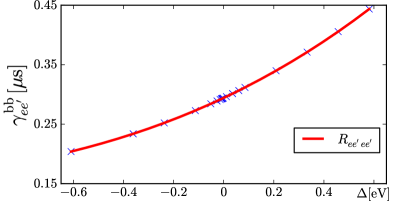
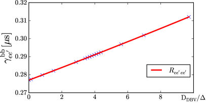
Figure 1: Left panel: $\gamma^{\mathrm{bb}}_{ee^{\prime}}$ as a function of the donor-acceptor excited state energy gap $\Delta$ (blue marks) and $R^{\mathrm{bb}}_{ee^{\prime}ee^{\prime}}$ as a function of $\Delta$ (red curve). Right panel: $\gamma^{\mathrm{bb}}_{ee^{\prime}}$ as a function of the ratio between the coupling strength $\textrm{D}_{\mathrm{DBV}}$ of the DBV-dimer and the energy gap $\Delta$ (blue marks) and $R^{\mathrm{bb}}_{ee^{\prime}ee^{\prime}}$ as a function of the ratio $\textrm{D}_{12}/\Delta$ (red curve). Other parameters are set to simulate the DBV dimer in Table 1 and with $T_{\mathrm{bb}}=5600$ K.

Further insight is afforded by Fig. 2. For the present case and at arbitrary temperature it is possible to identify two well-defined dynamical regimes: (i) A coherent regime for $\omega_{ee^{\prime}}>R^{\mathrm{bb}}_{ee^{\prime},ee^{\prime}}$ that guaranties that $L_{ee^{\prime}}$ has non-vanishing imaginary part and (ii) an incoherent regime for $\omega_{ee\prime}<R^{\mathrm{bb}}_{ee^{\prime},ee^{\prime}}$ that defines a purely real eigenvalue $L_{ee^{\prime}}$. The onset of the transition as a function of $R^{\mathrm{bb}}_{ee^{\prime},ee^{\prime}}$ coincides with that found for the case of a single chromophore above, as discussed in Eq. (21),

Figure 2: Real (blue marks) and imaginary (green marks) parts of eigenvalue $L_{ee^{\prime}}$ as a function of the transition dipole moment $\mu_{\mathrm{DBV}}$ of the DBV-dimer. The continuous red curve depicts $R^{\mathrm{bb}}_{ee^{\prime}ee^{\prime}}$ as a function of $\mu_{\mathrm{DBV}}$ whereas the dashed red curve does so for $2R^{\mathrm{bb}}_{ee^{\prime},ee^{\prime}}$. Other parameters are set to simulate the DBV dimer in Table 1 and with $T_{\mathrm{bb}}=5600$ K.

These estimates provide additional insight into the “underdamped” and “overdamped” regions noted previously Dodin et al. (2016b, a). From Figs. 1 and 2, it is clear that $R^{\mathrm{bb}}_{ee^{\prime}ee^{\prime}}$ accounts quantitatively for the decay rate $\gamma_{ee^{\prime}}^{bb}$ of the superposition between $|e\rangle$ and $|e^{\prime}\rangle$. Moreover, in the incoherent regime the transfer rate can be approximated by $2R^{\mathrm{bb}}_{ee^{\prime}ee^{\prime}}$.

In photosynthetic light-harvesting complexes (see Table 1), energy transfer occurs between eigenstates that are very close to one another, e.g., $\omega_{ab}\sim 10^{2}$cm^-1, and with transition dipole moments of the order of $10$ D. Thus, for isolated light-harvesting complexes, suddenly turned-on incoherent light induced dynamics are coherent (see below) provided that $\gamma^{\mathrm{bb}}_{ab}/\omega_{ab}<1$. By contrast, for atomic or molecular transitions with $\omega_{ab}$ on the order of $10^{3}$ cm^-1, with transition dipole moments on the order of $10$ D, incoherent dynamics are expected.

Figures 3 and 4 display the tensor elements $\chi_{ee^{\prime},gg}$, $\chi_{ee^{\prime},ee}$, $\chi_{ee^{\prime},e^{\prime}e^{\prime}}$, $\chi_{ee^{\prime},ff}$ for various cases associated with generating coherences in the singly excited manifold $\{e,e^{\prime}\}$ from incoherent initial states. Specifically, the left panel of Fig. 3 shows the results in the absence of blackbody radiation, i.e., the tensor elements $\chi^{\mathrm{tb}}_{ee^{\prime},aa}$, whereas the right panel displays the results in the absence of the thermal bath, i.e., the tensor elements $\chi^{\mathrm{bb}}_{ee^{\prime},aa}$. A number of significant features, and differences between blackbody and phonon baths, are evident. (i) The thermal bath introduced in Eq. (1) can not excite coherences in the singly excited manifold given population initially in the ground or doubly excited state; (ii) the tensor elements induced by the thermal bath in the singly excited manifold, $\chi^{\mathrm{tb}}_{ee^{\prime},ee}$ and $\chi^{\mathrm{tb}}_{e^{\prime}e^{\prime},aa}$, are five order of magnitude larger than those of blackbody radiation; (iii) the tensor elements induced by the thermal bath in the singly excited manifold, $\chi^{\mathrm{tb}}_{ee^{\prime},ee}$ and $\chi^{\mathrm{tb}}_{ee^{\prime},e^{\prime}e^{\prime}}$, decay far faster than those induced by blackbody radiation. This suggest that excitation with suddenly turned on incoherent light, can be considered as an effective coherent excitation over timescales less than the thermal bath decoherence times. (iv) The tensor elements $\chi^{\mathrm{tb}}_{ee^{\prime},ee}$ and $\chi^{\mathrm{tb}}_{ee^{\prime},e^{\prime}e^{\prime}}$ are out of phase with one another and the elements $\chi^{\mathrm{bb}}_{ee^{\prime},ee}$ and $\chi^{\mathrm{bb}}_{ee^{\prime},e^{\prime}e^{\prime}}$ oscillate in phase. This characteristic may well be relevant for identifying electronic from vibrational coherences in light-harvesting systems, a crucial problem in 2DPE light-harvesting experiments Tiwari et al. (2013).

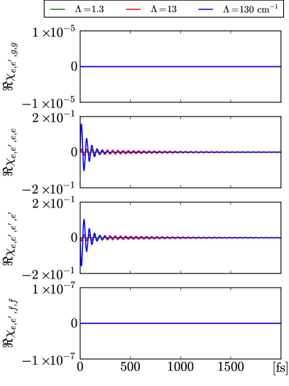
Figure 3: Left panel: Tensor elements $\chi^{\mathrm{tb}}_{ee^{\prime},aa}$ in the absence of blackbody radiation for different values of the reorganization energy $\Lambda$. Right panel: Tensor elements $\chi^{\mathrm{bb}}_{ee^{\prime},aa}$ in the absence of the thermal bath radiation for different values of the in site dipole transition moments $\mu$. Parameters are $T_{\mathrm{tb}}=300$ K, $T_{\mathrm{bb}}=5600$ K, and colour coding for different $\Lambda$ values is shown on top.

The left panel of Fig. 4 displays the results in the presence of both blackbody radiation and the thermal bath, i.e., the tensor elements $\chi^{\mathrm{tb+bb}}_{ee^{\prime},aa}$. The results are relatively insensitive to the dipole transition moments: increasing them by a factor of four, for example, gave qualitatively similar results.

The long time appearance of stationary coherences assisted by $\chi^{\mathrm{tb+bb}}_{ee^{\prime},gg}$ and $\chi^{\mathrm{tb+bb}}_{ee^{\prime},ff}$ is evident in the topmost and lowest panels in Fig. 4. In accord with Pachón and Brumer (2013); Pachon and Brumer (2013), the amplitude of these coherence increase with increasing coupling to the vibrations.

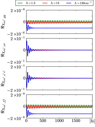
Figure 4: Tensor elements $\chi^{\mathrm{tb+bb}}_{ee^{\prime},aa}$ for different values of the reorganization energy $\Lambda$. Parameters are $T^{\mathrm{tb}}=300$ K, $T^{\mathrm{bb}}=5600$ K, and colour coding for different $\Lambda$ values is shown on top.

III.4 The PC645 antenna complex

For the multilevel system configuration discussed here [see Eq. (1)], and for the case of PC645, the dynamics grows in complexity due to the various dipole transitions induced by the incident light, and the multiple interactions between energy eigenstates excited by sunlight. For this multilevel configuration, the populations and decoherence rates are function of the coupling and energy gaps so that it is not straightforward to anticipate the behaviour of these rates. However, even this case, the approximation $\Re L^{\mathrm{bb}}_{ab}\sim R^{\mathrm{bb}}_{ab,ab}$ holds.

Excitation under model conditions. Consider first the case where all chromophores are initially in the ground state, and where they are initially decoupled from the environment (the latter is, indeed, an approximation, as discussed in detail in Pachón and Brumer (2013)), and where the suddenly turned on excitation by sunlight induces the dynamics.

For the ground state of PC645, the Hilbert space is spanned by 16 energy eigenstates $\{|e_{1}\rangle,|e_{2}\rangle,...|e_{16}\rangle\}$ with eigenvalues $e_{1}>e_{2}>...>e_{16}$. The single exciton manifold is spanned by the projectors $\{\left|e_{12}\left\rangle\right\langle e_{12}\right|,\left|e_{13}\left\rangle\right\langle e_{13}\right|,\left|e_{14}\left\rangle\right\langle e_{14}\right|,\left|e_{15}\left\rangle\right\langle e_{15}\right|\}$ which are delocalized over the sites. Excitations in chromophores DBVd or DBVc would correspond to populations in $\left|e_{12}\left\rangle\right\langle e_{12}\right|$ and $\left|e_{13}\left\rangle\right\langle e_{13}\right|$, while excitations in the chromophores MBVb and MBVa mainly involve $\left|e_{14}\left\rangle\right\langle e_{14}\right|$ and $\left|e_{15}\left\rangle\right\langle e_{15}\right|$.

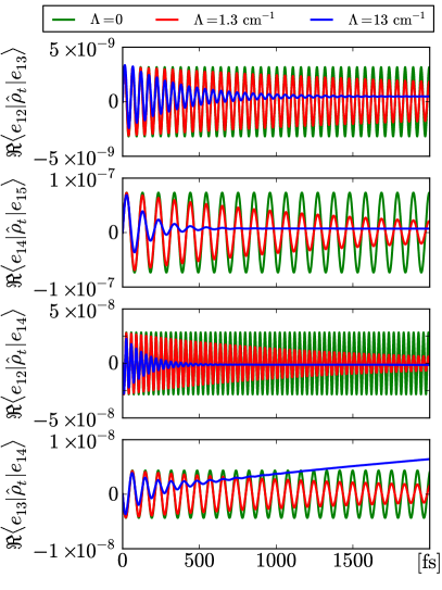
Figure 5: Left panel: Time evolution at room temperature of the states associated with the single exciton manifold for different values of $\Lambda$. Right panel: Time evolution at room temperature of coherences of sample superpositions between single-exciton-manifold states induced by suddenly turned on sunlight. Parameters are $\lambda=100$ cm^-1, $T_{\mathrm{env}}=300$ K, $T_{\mathrm{bb}}=5600$ K and $\hat{\rho}(t=0)=\left|e_{16}\left\rangle\right\langle e_{16}\right|$, i.e., in the ground state.

Figure 5 shows the time evolution of the populations of the eigenstates associated with the single exciton manifold as well as some of the coherent superpositions prepared between these states by suddenly turned on incoherent light (sunlight). The observed linear population growth is expected in low intensity incoherent light. If there is no coupling to the local environments ($\Lambda=0$), suddenly turned on sunlight is seen to prepare coherent superpositions that last for hundreds of picoseconds. However, the amplitude of the coherences is approximately two orders of magnitude smaller than that of the excited state population and so becomes irrelevant quicklySadeq and Brumer (2014). Further, when the coupling to the environment is included ($\Lambda\neq 0$), the coherent superpositions maintained in sunlight decay due to the underlying incoherent dynamics of the local environment. In this case, due to the initial condition (all the population in the ground state), no coherences between the ground state and the excited states are present, i.e., coherences in this case are among excited states.

The left panel of Fig. 5 also displays an interesting dependence on $\Lambda$. For example, for $\langle e_{12}|\hat{\rho}_{t}|e_{12}\rangle$ absorption increases with increasing value of $\Lambda$, whereas the opposite is the case for $\langle e_{13}|\hat{\rho}_{t}|e_{13}\rangle$. These considerable differences in the state populations are a manifestation of the effect of the coupling of the system to the bath and the associated flow of population between eigenstates and trace preservation of $\hat{\rho}(t)$.

Also of interest is the behaviour of populations and coherences as viewed from the site basis. To this end, we have transformed from the eigenstate to the site basis, denoted $\{|\epsilon_{1}\rangle,|\epsilon_{2}\rangle,\ldots\}$. In this basis the single exciton manifold is spanned by the projectors $\{\left|\epsilon_{8}\left\rangle\right\langle\epsilon_{8}\right|,\left|\epsilon_{12}\left\rangle\right\langle\epsilon_{12}\right|$, $\left|\epsilon_{14}\left\rangle\right\langle\epsilon_{14}\right|,\left|\epsilon_{15}\left\rangle\right\langle\epsilon_{15}\right|\}$, which correspond to the chromophores MBVa, MBVb, DBVc and DBVd, respectively. Figure 6 shows the time evolution of site-basis matrix elements associated with the single exciton manifold presented in Fig. 5.

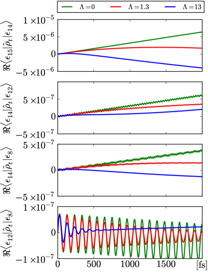
Figure 6: Description and parameters as in Fig. 5 but with matrix elements in the site basis. Note that the populations of the states $\{|\epsilon_{8}\rangle\langle\epsilon_{8}|,|\epsilon_{12}\rangle\langle\epsilon_{12},|\epsilon_{14}\rangle\langle\epsilon_{14},|\epsilon_{15}\rangle\langle\epsilon_{15}\}$ refer to the chromophores MBVa, MBVb, DBVc and DBVd, respectively.

In this case, coherences are approximately an order of magnitude larger than in the exciton basis, but the populations are of similar magnitude. Hence, the coherences become negligible as time progresses.

One note is in order. For larger values of the reorganization energy $\Lambda$, stationary coherences in the long-time limit in the eigenstate basis are expected to be larger Pachón and Brumer (2013). These coherences are a direct consequence of the coupling of the electronic degree of freedom to the vibrational bath Pachón and Brumer (2013) discussed above. Since the focus here is on the nature of the excited states prepared by sunlight, larger values of the reorganization values are not considered.

Energy pathways under incoherent and coherent radiation. As we have previously argued Brumer and Shapiro (2012) dynamics observed in pulsed laser experiments is distinctly different from that observed in nature due to the coherence characteristics of the incident light. Here we note a second significant difference arising from the incident spectrum of the light. In particular, 2DPE studies have focused on the spectral region associated with absorption in the DBV_- state (see the Fig. 1.C in Ref. Collini et al. (2010)), with energy then flowing towards the MBV molecules Collini et al. (2010). However, in absence of vibrations, as shown below, this is not the only pathway associated with natural light absorption, where the excitation has a wider frequency spectrum.

For example, for the ideal unitary case of $\Lambda=0$ in Fig. 6, it is clear that the four chromophores DBVc, DBVd, MBVa, MBVb show essentially the same rate of population growth, all reaching $\sim 5\times 10^{-6}$ in 1 ps.

Figure 7: Time evolution the states associated with the single exciton manifold in the site basis with no coupling of the MBV molecules to the thermal light and with $\Lambda=0$ (left panel) and $\Lambda=13$ cm^-1 (right panel). Note the log-scale of the y-axis.

Hence, excitation with thermal light is completely different than that of pulses due to its broad spectrum, which simultaneously excites the four chromophores in accord with the magnitude of the transition dipole moment (see Table 1). For example, excitation of the MBV molecules in Fig. 6 is due to both direct excitation by the light as well as energy transfer. Figure 7 quantifies each contribution by showing the dynamics of the populations when the coupling of the MBV molecules to the light is turned off for $\Lambda=0$ (left panel) and $\Lambda=13$ cm^-1 (right panel). For $\Lambda=0$, at 2 ps, the population of the MBV molecules is ca. three orders of magnitude smaller than the population obtained when the direct interaction with light is included (see Fig. 6). For $\Lambda=13$ cm^-1, a significant increment in the population of MBV molecules is achieved, ca. two orders of magnitude. This points out the important role of vibrations in exciton energy transfer even under incoherent excitation. This is made even all the more evident when examining the case of $\Lambda=130~{}\mathrm{cm}^{-1}$, a value suggested experimentally for the PC645 system and shown in Fig.  8. Here (by comparison with extrapolated results from Fig. 6) excited MBV population arising from direct MBV excitation and from DBV to MBV transfer are seen to be comparable in size.

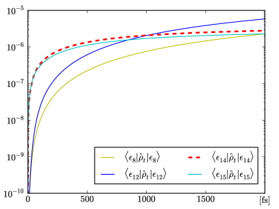
Figure 8: Time evolution the states associated with the single exciton manifold in the site basis with no coupling of the MBV molecules to the thermal light and with $\Lambda=130$ cm^-1. Note the log-scale of the y-axis.

III.5 The Requirement for Proper Preparation

Several studies have been published that ignore the preparation step, where the system is excited by light, and consider that the system starts in a given excited state, after which the dynamics follows. For example, in the PC645 case such a study Fassioli et al. (2012) assumed that the sunlight had prepared the system in eigenstates where the excitations of DBVc and DBVd are mainly resident. The subsequent effect of sunlight is included via a master equation of the Lindblad form with a decay rate $\Gamma_{\mathrm{Lindblad}}^{-1}\sim 250$ ps. Our approach allows us to assess the relevance of this preparation step to the natural light-induced process.

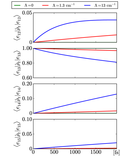
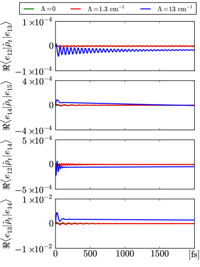
Figure 9: Left panel: Time evolution at room temperature of the states associated with the single exciton manifold for different $\Lambda$ values. Right panel: Time evolution at room temperature of several of the superpositions between single-exciton-manifold states induced by sunlight. Parameters are $\lambda=100$ cm^-1, $T_{\mathrm{env}}=300$ K, $T_{\mathrm{bb}}=5600$ K and $\hat{\rho}(t=0)=\left|e_{13}\left\rangle\right\langle e_{13}\right|$.

Consider then the case introduced in Fassioli et al. (2012) where the antenna is artificially prepared in the excited eigenstate $\left|e_{13}\left\rangle\right\langle e_{13}\right|$ and the interaction with sunlight and the local environment is then switched on, defining $t=0$. Figures 9 and 10 show the resultant dynamics in the eigenstate and the site basis, respectively. Note first that the amplitude of the population and the coherences are approximately five orders of magnitude larger here than in the case of natural excitation. This implies that the artificial initial condition $\hat{\rho}(t=0)=\left|e_{13}\left\rangle\right\langle e_{13}\right|$ strongly activates the subsequent interaction with the environment. That is, under these conditions the dynamics is dominated by the environment, with marginal influence of the radiation. To quantify this statement, we calculate the trace distance $\mathcal{D}(\hat{\rho},\hat{\rho}_{\hat{\bm{\mu}}=0})=\mathrm{tr}|\hat{\rho}-\hat{\rho}_{\hat{\bm{\mu}}=0}|$ between the density operator driven by the (environment + sunlight) $\hat{\rho}$, and the density operator driven only by the environment, $\hat{\rho}_{\bm{\mu}=0}$. For orthogonal states, i.e., completely distinguishable states, the trace distance would be one. For the cases depicted in Figs. 9 and 10, the trace distance is of the order of $10^{-15}$. This clearly demonstrates that the effect of the radiation is negligible in this case. That is, the coherences observed in Fig. 9 have nothing to do with sunlight but are generated by the non-equilibrium initial condition Pachón and Brumer (2013), contrary to an earlier incorrect assertion Fassioli et al. (2012). It also emphasizes the need to properly include the radiative excitation step to study dynamics induced by incoherent light, as done in this paper.

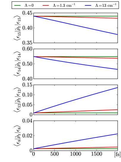
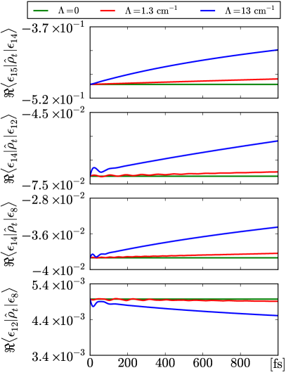
Figure 10: Description and parameters as in Fig. 9 but with matrix elements are in the site basis.

IV Summary

An open systems quantum perspective is adopted to examine the excitation, via incoherent light, of systems imbedded in a bath. Specifically, the nature and role of the quantum dynamical maps are analyzed in detail for model components of light harvesting systems. Contrasts between the effect of the radiative bath and the phonon bath are analyzed. In particular, phonon-bath dephasing times are found to be far longer in the radiative case than in the phonon case due to well described differences in system-bath coupling and bath spectral densities. Examination of increasingly complicated models of components of the PC645 light harvesting complex shows the appearance of oscillatory and stationary coherences, the significance of multichromophoric excitation that occurs naturally as distinct from localized chromophore excitation that is carried out in the laboratory, and the importance of properly treating the light-excitation step to model the true dynamics. The approach provides a direct means of analyzing a wide variety of initial conditions within one formalism.

Acknowledgements—This work was supported by the US Air Force Office of Scientific Research under contract number FA9550-13-1-0005, by Comité para el Desarrollo de la Investigación (CODI) of Universidad de Antioquia, Colombia under the Estrategia de Sostenibilidad and the Purdue-UdeA Seed Grant Program and by the Departamento Administrativo de Ciencia, Tecnología e Innovación (COLCIENCIAS) of Colombia under the contract number 111556934912.

Appendix A Slow Turn-On of the Light

To simulate the slow turn-on of the light, it is convenient to introduce a time dependence of the transition dipole moments, namely, $\bm{\mu}_{ab}=\bm{\mu}_{ab}\mathrm{Erf}_{ab}(t)$, with

$$\mathrm{Erf}_{12,13}(t)=\frac{2}{\sqrt{\pi}}\int_{0}^{|\omega_{12,13}|t/\alpha}\mathrm{d}z\exp(-z^{2}).$$ (24)

For large $\alpha\gg 1$ this can be approximated by $\mathrm{Erf}_{12,13}(t)\sim\frac{2|\omega_{12,13}|}{\pi\alpha}t$. Thus, $2|\omega_{12,13}|/\pi\alpha$ can be interpreted as the rate of light turning-on. The method introduces the turn-on rate into the dipole coupling and is different from that advanced in Ref. Dodin et al. (2016a), where the field populations are altered, but should give similar results.

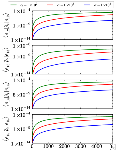
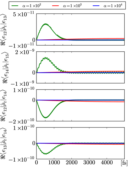
Figure 11: Time evolution at room temperature of the populations (left panels) and coherences (right panels) associated with the single exciton manifold for different values of $\alpha$ with $\Lambda=0$. Parameters as in Fig. 5.

Figure 11 depicts the time evolution of the single exciton manifold of the PC645 sub-unit discussed above. Clearly, the slower the turn-on the smaller the coherences.

References

- Engel et al. (2007) G. S. Engel, T. R. Calhoun, E. L. Read, T.-K. Ahn, T. Mančal, Y.-C. Cheng, R. E. Blankenship, and G. R. Fleming, Nature 446, 782 (2007).
- Collini et al. (2010) E. Collini, C. Y. Wong, K. E. Wilk, P. M. G. Curmi, P. Brumer, and G. D. Scholes, Nature 463, 644 (2010).
- Jiang and Brumer (1991) X.-P. Jiang and P. Brumer, J. Chem. Phys. 94, 5833 (1991).
- Mančal and Valkunas (2010) T. Mančal and L. Valkunas, New J. Phys. 12, 065044 (2010).
- Brumer and Shapiro (2012) P. Brumer and M. Shapiro, Proc. Natl. Acad. Sci. U.S.A. 109, 19575 (2012), arXiv:1109.0026 [quant-ph] .
- Chenu and Brumer (2016) A. Chenu and P. Brumer, J. Chem. Phys. 144, 044103 (2016).
- Fassioli et al. (2012) F. Fassioli, A. Olaya-Castro, and G. D. Scholes, J. Phys. Chem. Lett. 3, 3136 (2012).
- Pachón and Brumer (2013) L. A. Pachón and P. Brumer, Phys. Rev. A 87, 022106 (2013), arXiv:1210.6374 .
- Kassal et al. (2013) I. Kassal, J. Yuen-Zhou, and S. Rahimi-Keshari, J. Phys. Chem. Lett. 4, 362 (2013).
- Han et al. (2013) A. C. Han, M. Shapiro, and P. Brumer, J. Phys. Chem. A 117, 8199 (2013).
- Pachón and Brumer (2014) L. A. Pachón and P. Brumer, J. Math. Phys. 55, 012103 (2014), arXiv:arXiv:1207.3104 .
- Chenu et al. (2014) A. Chenu, P. Malý, and T. Mančal, Chem. Phys. 439, 100 (2014).
- Chenu et al. (2014) A. Chenu, A. M. Brańczyk, G. D. Scholes, and J. E. Sipe, ArXiv e-prints (2014), arXiv:1409.1926 [quant-ph] .
- Sadeq and Brumer (2014) Z. S. Sadeq and P. Brumer, J. Chem. Phys. 140, 074104 (2014).
- Pelzer et al. (2014) K. M. Pelzer, T. Can, S. K. Gray, D. K. Morr, and G. S. Engel, J. Phys. Chem. B 118, 2693 (2014).
- Pachón and Brumer (2011) L. A. Pachón and P. Brumer, J. Phys. Chem. Lett. 2, 2728 (2011), arXiv:1107.0322v2 .
- Tscherbul and Brumer (2014) T. V. Tscherbul and P. Brumer, Phys. Rev. Lett. 113, 113601 (2014).
- Dodin et al. (2016a) A. Dodin, T. V. Tscherbul, and P. Brumer, J. Chem. Phys. 145, 244313 (2016a).
- Mandel and Wolf (1995) L. Mandel and E. Wolf, Optical coherence and quantum optics (Cambridge University Press, Cambridge, 1995).
- May and Kühn (2001) V. May and O. Kühn, Charge and energy transfer dynamics in molecular systems (Berlin: Wiley, 2001).
- Pachón et al. (2013) L. A. Pachón, L. Yu, and P. Brumer, Faraday Discussions 163, 485 (2013), arXiv:1212.6416 .
- Pachon and Brumer (2014a) L. A. Pachon and P. Brumer, J. Chem. Phys. 141, 174102 (2014a).
- Ford et al. (1985) G. W. Ford, J. T. Lewis, and R. F. O’Connell, Phys. Rev. Lett. 55, 2273 (1985).
- Pachon and Brumer (2014b) L. A. Pachon and P. Brumer, J. Mathem. Phys. 55, 012103 (2014b).
- Pachon et al. (2015) L. A. Pachon, A. H. Marcus, and A. Aspuru-Guzik, J. Chem. Phys. 142, 212442 (2015), arXiv:1502.02363 [quant-ph] .
- Pachon and Brumer (2013) L. A. Pachon and P. Brumer, J. Chem. Phys. 139, 164123 (2013).
- Mirkovic et al. (2007) T. Mirkovic, A. B. Doust, J. Kim, K. E. Wilk, C. Curutchet, B. Mennucci, R. Cammi, P. M. G. Curmi, and G. D. Scholes, Photochem. Photobiol. Sci. 6, 964 (2007).
- Jefferts et al. (2014) S. R. Jefferts, T. P. Heavner, T. E. Parker, J. H. Shirley, E. A. Donley, N. Ashby, F. Levi, D. Calonico, and G. A. Costanzo, Phys. Rev. Lett. 112, 050801 (2014).
- Dodin et al. (2016b) A. Dodin, T. V. Tscherbul, and P. Brumer, J. Chem. Phys. 144, 244108 (2016b).
- Harrop et al. (2014) S. J. Harrop, K. E. Wilk, R. Dinshaw, E. Collini, T. Mirkovic, C. Y. Teng, D. G. Oblinsky, B. R. Green, K. Hoef-Emden, R. G. Hiller, G. D. Scholes, and P. M. G. Curmi, Proc. Natl. Acad. Sci. USA 111, E2666 (2014).
- Tiwari et al. (2013) V. Tiwari, W. K. Peters, and D. M. Jonas, Proc. Natl. Acad. Sci. U.S.A. 110, 1203 (2013).