Statistical Topology and the Random Interstellar Medium

Abstract

Current astrophysical models of the interstellar medium assume that small scale variation and noise can be modelled as Gaussian random fields or simple transformations thereof, such as lognormal. We use topological methods to investigate this assumption for three regions of the southern sky. We consider Gaussian random fields on two-dimensional lattices and investigate the expected distribution of topological structures quantified through Betti numbers. We demonstrate that there are circumstances where differences in topology can identify differences in distributions when conventional marginal or correlation analyses may not. We propose a non-parametric method for comparing two fields based on the counts of topological features and the geometry of the associated persistence diagrams. When we apply the methods to the astrophysical data, we find strong evidence against a Gaussian random field model for each of the three regions of the interstellar medium that we consider. Further, we show that there are topological differences at a local scale between these different regions.

Keywords: astrophysics, Betti numbers, convex hull, filamentarity, nonparametric test, persistence diagram, random field.

1 Introduction

The stars of the Milky Way and other galaxies are embedded in the interstellar medium (ISM), a mixture of gas, cosmic rays and magnetic fields. The ISM is an important and active ingredient in the Galactic system despite comprising only about $10\%$ of the total baryonic mass of the Galaxy (Ferrière, 2001). New stars form from cold, dense, parts of the ISM, while stellar evolution driven by energy release from thermonuclear reactions returns some of the stellar mass to the ISM via stellar winds and supernova explosions. This injection of energy generates turbulent motions and shocks in the ISM, producing a highly heterogeneous random structure. Accurate knowledge of the spatial distribution of the ISM is required to understand the properties and evolution of galaxies.

One way to probe the ISM is to observe neutral atomic hydrogen (H i), as about $90\%$ of atoms in the interstellar gas are hydrogen (Kalberla & Kerp, 2009). H i emits and absorbs radio waves at the frequency of $1420$ MHz and large data sets are now available for detailed analysis. Figure 1 shows H i distribution in a section of the southern sky. These data were obtained by the Galactic All-Sky Survey (GASS) using the Parkes $64\,{\rm m}$ radio telescope (McClure-Griffiths et al., 2009; Kalberla et al., 2010). The second and third releases of the data are available at http://www.astro.uni-bonn.de/hisurvey. The figure shows the antenna-temperature distribution $T(l,b)$, which is related to the gas density, as a function of position on the sky, using the coordinates of Galactic longitude, $l$, and latitude, $b$. The distance to the gas cannot be measured directly, but the Doppler-shift of the emission, dominated by the differential rotation of the Galaxy, produces a line-of-sight velocity $v$ that can in principle be used to determine the location of the gas in three dimensions. The transformation is complicated, however, and not necessary for our purposes. Instead, we obtained the two-dimensional data in Figure 1 by integrating $T$ over velocities from $v=20.6$ to $v=40.4\,{\rm km/s}$.

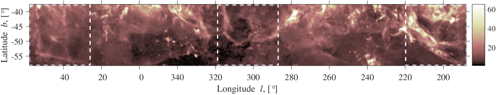
Figure 1: Emission of neutral atomic hydrogen H i in a region of the Southern sky (McClure-Griffiths et al., 2009). The coordinates are Galactic longitude $l$ and latitude $b$, centered on the Sun, where the mid-plane of the Galactic disc is at $b=0^{\circ}$ and the Galactic centre is in the direction $l=0^{\circ}$. The brightness temperature shown is proportional to the total mass of H i along the line of sight. Dashed squares from left to right identify the Regions 1–3 used in Section 6.

The GASS data and other surveys are rich enough to allow subtle comparisons between observations and the results of sophisticated magneto-hydrodynamic (MHD) simulations of the ISM. The data are represented as random fields with large-scale gradients and a complex topology widely believed to be related to turbulence and outflows from the Galactic disk. At a more local level, Gaussian random fields (GRF), or simple transformations thereof, have underpinned the modelling of small-scale variations in H i. In this paper we investigate whether these models are sufficient to describe the small-scale properties of $T(l,b)$.

We consider the three regions marked by dashed lines in Figure 1, which we refer to as Regions 1–3, moving from left to right. Each consists of a $256\times 256$ array of temperature values. The selection of the regions was arbitrary: we did not consider any astronomical information about the locations when drawing their boundaries. In order to concentrate on small-scale variation we removed the trend from the plots by fitting to each region a polynomial surface of order four in each of $l$ and $b$. The residuals were then marginally transformed to N(0,1). If this transformation results in a realisation of a GRF then all information would be captured by the correlation function. We therefore consider two questions.

1. Q1. Are the transformed data sets consistent with stationary isotropic Gaussian random fields?

2. Q2. Are there differences between the three data sets, to which the correlation function is insensitive?

We will address both questions using techniques in topological data analysis, which is becoming a popular approach to the analysis of random fields and more generally (Adler et al., 2010; Adler & Taylor, 2011; Bubenik, 2015; Carlsson, 2009; Edelsbrunner, 2014; Fasy et al., 2014; Yogeshwaran & Adler, 2015). Topological invariants such as Betti numbers, the Euler characteristic, persistence diagrams and persistence barcodes, rank functions and landscapes, have been used in areas such as astrophysics (Li et al., 2016), cosmology (Gay et al., 2010; Sousbie, 2011; Sousbie et al., 2011; Pranav, 2015), fluid dynamics (Kramár et al., 2016; Li et al., 2016) and medicine (Davis, 2008; Chung et al., 2009, 2015). A difference in our case compared with most previous work however is that we have just a single observation for each region, so that inferential techniques based on sampling and asymptotics are not appropriate.

In Section 2 we describe several topological summaries that are appropriate for data on two-dimensional lattices. In Section 3 we study characteristics when a GRF is appropriate. In Section 4 we demonstrate that non-Gaussian random fields can sometimes be distinguished by topological features even though first and second order properties (marginal distribution and correlation function) are the same. In Section 5 we propose a simple procedure for comparing two single realisations of random fields and in Section 6 we describe our analysis of the GASS data.

2 Topological descriptors of a random field

Here we describe a number of topological measures that are suitable for analysing data that are distributed on a two-dimensional rectangular lattice. For more general definitions and interpretations and further information see, for instance, Adler et al. (2004); Bubenik (2015) or Fasy et al. (2014).

2.1 Level sets, persistent homology and persistence diagrams

Let $z(x)$ be the value of a random field at location $x$ on a two-dimensional lattice. For any real $t$, the lower-level set is defined as the locations that have field values below $t$,

$$\mathcal{F}_{t}=\{x:z(x)\leq t\}.$$

Increasing $t$ from below defines a filtration which is used in persistent homology to describe the evolution of topological structures in the field. In our context, there are two topological features of interest, namely components and holes, whose counts in a level set determine the Betti numbers of order zero and one, $\beta_{0}$ and $\beta_{1}$, respectively (Carlsson, 2009). Figure 2 shows four lower-level sets for a simulated field on a $10\times 10$ lattice and will be used to illustrate some basic concepts.

Figure 2: Four level sets (black) for a field on a $10\times 10$ lattice.

A component is a group of one or more pixels in a lower level set that are connected to each other, where for now we define neighbouring pixels to be connected if they have a common edge, and non-neighbouring pixels to be connected if there is a path of connected neighbours between them. The Betti number of order zero, $\beta_{0}$, for $\mathcal{F}_{t}$ is the number of components in the level set. In Figure 2 for instance, in panel (a) at $t=-2$ we have $\beta_{0}=3$, as we have assumed that pixels that share only a vertex are not connected. By $t=-1$ and panel (b) we have $\beta_{0}=7$, and then $\beta_{0}=5$ and $\beta_{0}=1$ in panels (c) and (d) respectively. The emergence of a new component is described as a birth and the merger of two components is interpreted as the continuation of the component with the earlier birth time and the death of the other. In a two-dimensional field each local minimum is associated with the birth of a component.

A hole is a group of one or more pixels that are not in the level set, are connected to each other but are isolated from other pixels that are also outside the level set. The Betti number of order one, $\beta_{1}$, for $\mathcal{F}_{t}$ is the number of holes in the level set. Thus in panel (d) of Figure 2 we have $\beta_{1}=9$ as we ignore common vertices. In panel (c) we have $\beta_{1}$=5, in (b) $\beta_{1}=2$ and in (a) we have $\beta_{1}=1$. New holes are created when existing ones split, and again we can define their birth and death levels $t$. The death of a hole is associated with a local maximum. Holes could alternatively be defined by symmetry as components in a similarly defined upper level set, with the filtration now running from high to low $t$. We will always refer to lower level sets so as to avoid confusion.

A persistence diagram is a scatterplot of birth levels against death levels for features of interest, in our case either components or holes. The left plot of Figure 3 shows a persistence diagram for components in Region 1 of the transformed GASS data. The first component to be born is by construction the last to die, producing the single point in the top left. Otherwise, the points are clustered in a loose oval. Points near the diagonal represent less persistent structures mostly associated with noise, whereas more significant features are usually associated with points away from the diagonal.

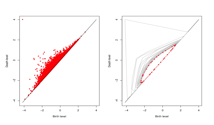
Figure 3: Component persistence diagram (left) and 90% convex peel (right, as dots) for Region 1 in the GASS data. Grey lines in the right panel represent the peeled convex hulls.

2.2 Convex peels and summary statistics

It is sometimes difficult to interpret or compare persistence diagrams, either because of the large number of points or the bunching of many points along the diagonal. We propose peeling successive convex hulls (Barnett, 1976) until only a prescribed proportion of points remain, as illustrated in the right panel of Figure 3. In this way we extract the general shape of the persistence diagram without undue influence of either outliers or the mass of points near the boundary. We summarise the shape of the final convex hull by the following five statistics:

1. the two centroid coordinates $(C_{b},C_{d})$;

2. the perimeter $P$;

3. the area $A$;

4. the filamentarity, defined as (Bharadwaj et al., 2000; Makarenko et al., 2015)

   $$F=\frac{P^{2}-4\pi A}{P^{2}+4\pi A},\;\;\;\;\;\;\;0\leq F\leq 1.$$

   Thus defined, $F=0$ for a circle and $F=1$ for a line.

2.3 Bottleneck distance

The bottleneck distance provides a measure in the space of persistence diagrams and can be used as a quantitative summary of the difference between two persistence diagrams, $A$ and $B$ say. A readable description, and further information, is given by Fasy et al. (2014).

First, the points in $A$ are matched to the points in $B$. This means that each point in $A$ is mapped either to a unique point in $B$, or to its projection onto the diagonal line of birth-death equality. The same is true for $B$. Use of the diagonal is necessary because $A$ and $B$ can have different numbers of points.

The cost of a mapping from a point $(a_{ix},a_{iy})$ in $A$ to a point $(b_{jx},b_{jy})$ in $B$ is the norm

$$c_{ij}=\max\{\mid a_{ix}-b_{jx}\mid,\;\mid a_{iy}-b_{jy}\mid\}.$$

The total cost of a matching $P$ between $A$ and $B$ is $C(P)=\sum_{i,j}c_{ij}$. The bottleneck distance is then

$$w(A,B)=\min_{P}C(P),$$

where the minimum is taken over all possible selections of the linked pairs. This, the bottleneck distance, is essentially the smallest cost that could be incurred in mapping all points of $A$ into all points of $B$. Calculation is numerically expensive, though efficient algorithms are available. For our application, we used the tda package in R.

3 Topology of a Gaussian random field on a lattice

The persistent homology of a two-dimensional random field depends upon the number and distribution of local maxima and minima. In this section, we investigate the number of local extrema in a Gaussian random field on a $d\times d$ lattice. The results will be used in Section 6 to benchmark an analysis of the H i data. We assume stationarity, isotropy and N(0,1) margins throughout.

The density of critical points of a Gaussian random field in continuous space is a well-studied problem (Bardeen et al., 1986). It depends upon the joint Gaussian distribution of function values and first and second derivatives. We are not aware of published results for local extrema of a field on a discrete lattice however, although there has been work on the distribution of the global maximum over a region (Taylor et al., 2007).

3.1 Expected number of local extrema

Given a field $z(x)$, let $N_{0}$ and $N_{1}$ be the numbers of points in persistence diagrams for components and holes respectively. As previously stated, each point in a persistence diagram for components corresponds to a local minimum of the field, and each point in a persistence diagram for holes corresponds to a local maximum. Due to the symmetry of the Gaussian distribution, the number of local minima has the same statistical properties as the number of local maxima. Because it is slightly tidier notationally, we will consider local maxima in this section.

Let $z_{1}=z(x_{1})$ be the (scalar) field value at some location $x_{1}$ and let $z_{2}=z(x_{2})$ be the $k$-dimensional vector of field values at the immediate neighbours $x_{2}$ of $x_{1}$, with the neighbourhood to be defined later. Then, because we have standardised, $(z_{1},z_{2})$ is Gaussian, with zero mean and variance matrix

$$\left(\begin{array}[]{cc}1&r^{T}\\ r&R\end{array}\right).$$

Here the $k$-vector of correlations $r$ between $z_{1}$ and $z_{2}$, and the $k\times k$ correlation matrix $R$ of $z_{2}$, each depend on the locations $x_{1}$ and $x_{2}$, though this is suppressed in the notation.

We have a local maximum at $x_{1}$ if $z_{2}<z_{1}1_{k}$ where $1_{k}$ is a $k-$vector of ones. We can calculate this from the conditional distribution of $z_{2}$ given $z_{1}$ and the marginal distribution of $z_{1}$. First let $\phi^{(p)}(x;\mu,\Sigma)$ be the $p$-dimensional Gaussian probability density with mean vector $\mu$ and covariance matrix $\Sigma$, with $\Phi^{(p)}(x;\mu,\Sigma)$ being the corresponding cumulative distribution function. So $z_{1}$ has density $\phi^{(1)}(z_{1};0,1)$, $z_{2}$ has density $\phi^{(k)}(z_{2};0_{k},R)$, where $0_{k}$ is a $k-$vector of zeros, and the conditional density for $z_{2}$ given $z_{1}$ is

$$\phi^{(k)}(z_{2};rz_{1},R-rr^{T}).$$

Then

$$p_{1}=P(\mbox{local maximum at }x_{1}) = P(z_{2}<z_{1}1_{k})$$

$$= \int_{z_{1}}\left\{\int_{z_{2}<z_{1}1_{k}}\phi^{(k)}(z_{2};rz_{1},R-rr^{T})\,dz_{2}\right\}\phi^{(1)}(z_{1};0,1)\,dz_{1}$$

$$= \int_{z_{1}}\Phi^{(k)}(z_{1}1_{k};rz_{1},R-rr^{T})\phi^{(1)}(z_{1};0,1)\,dz_{1}$$

$$= \int_{z_{1}}\Phi^{(k)}((1_{k}-r)z_{1};0_{k},R-rr^{T})\phi^{(1)}(z_{1};0,1)\,dz_{1}.$$

A general skew-Normal distribution described by Gupta et al. (2004); Azzalini (2005); Arnold (2009) and Barrett et al. (2014) can be used to show that

$$\Phi^{(q)}(D\mu;\nu,\Delta+D\Sigma D^{T})=\int_{y}\Phi^{(q)}(Dy;\nu,\Delta)\phi^{(p)}(y;\mu,\Sigma)\,dy,$$ (1)

where $\mu$ is of dimension $p$, $\nu$ is of dimension $q$, $\Sigma$ and $\Delta$ are $p\times p$ and $q\times q$ covariance matrices respectively, and $D$ is an arbitrary $q\times p$ matrix. Hence, if we set

$$p=1,\;\;\;q=k,\;\;\;\mu=0,\;\;\;\Sigma=1,\;\;\;\nu=0_{k},\;\;\;\Delta=R-rr^{T},\;\;\;y=z_{1}\mbox{ and }D=1_{k}-r,$$

then

$$p_{1} = \Phi^{(k)}(0_{k};0_{k},R-rr^{T}+(1_{k}-r)(1_{k}-r)^{T})$$ (2)

$$= \Phi^{(k)}(0_{k};0_{k},R+1_{k}1_{k}^{T}-1_{k}r^{T}-r1_{k}^{T}).$$

Summing over all locations yields $E[N_{1}]=E[N_{0}]=\sum_{j}p_{j}$, where $p_{j}$ is obtained from the equivalent of (2) for location $x_{j}$ instead of $x_{1}$. To calculate, we next need to define the neighbourhood of a lattice node. Thinking of a lattice as an array of square pixels, those with common boundaries are clearly neighbours. With this choice, an interior pixel thus has $k=4$ neighbours, with differences in location of the form $(\pm 1,0)$ or $(0,\pm 1)$. We will call this the cross neighbourhood, which is what was used in the discussion of connected locations in Section 2.1. We may alternatively consider in addition pixels that share at least one vertex as neighbours. An interior pixel then has $k=8$ neighbours, consisting of the previous four and the four corners $(\pm 1,\pm 1)$. We will call this the square neighbourhood.

Table 1 shows $E[N_{1}]$ for three different grid sizes, assuming exponential correlation function with correlation length (the integral of the correlation function) equal to 20, which is close to that in the H i data. We used the pmvnorm routine in the mvtnorm package within R, with the Miwa algorithm to calculate $\Phi^{(k)}$, and we adjusted neighbourhoods appropriately for pixels on boundaries. The table also gives the means and associated standard errors of counts from 1000 simulations in each case. The simulation results match the analytical results well. For larger correlation lengths of $z(x)$ (not shown), there are fewer maxima or minima for a fixed size lattice, and the opposite for shorter correlation lengths. At zero correlation length, the number of minima (or maxima) is about 1/5 of the total number of points for the cross neighbourhood, and 1/9 for the square, as expected.

Table 1: Expected number of local maxima for a discrete Gaussian random field on a $d\times d$ lattice, with exponential correlation function of correlation length 20. The simulation results are the means (standard errors) from 1000 repetitions.

	Neighbourhood
	Cross, $k=4$		Square, $k=8$
	Simulation	Eq.(2)	Simulation	Eq.(2)
$d=32$	128.3	128.4	68.8	68.9
	(0.3)		(0.2)
$d=64$	498.3	497.9	258.3	258.3
	(0.5)		(0.4)
$d=256$	7786.7	7786.5	3927.4	3929.5
	(2.2)		(1.6)

3.2 Variance of number of local extrema

Let $I_{j}$ be an indicator of a local maximum at location $x_{j}$. In order to determine the variance of $N_{1}=\sum I_{j}$ we need $E[I_{i}I_{j}]$ for all pairs of locations $x_{i}$ and $x_{j}$. First we introduce some notation. Let $z_{1}=(z_{11}(x_{11}),z_{12}(x_{12}))$ be the (bivariate) field value at any two locations $x_{11}$ and $x_{12}$. Let $z_{21}(x_{21})$ be the $k_{1}$-dimensional vector of field values over the neighbours $x_{21}$ of $x_{11}$, and let $z_{22}(x_{22})$ be the $k_{2}$-dimensional vector of field values over the neighbours $x_{22}$ of $x_{12}$. Finally, let $z_{2}$ be the $(k_{1}+k_{2})$-vector made up of $z_{21}(x_{21})$ and $z_{22}(x_{22})$.

We need to consider separately the three possible arrangements of the neighbours: first, when $x_{11}$ and $x_{12}$ have no common neighbours; second, when a neighbour is shared between $x_{11}$ and $x_{12}$; and third, when one of $x_{11}$ and $x_{12}$ is itself in the neighbourhood of the other. In the first case, of no common neighbours, $x_{21}$ and $x_{22}$ are distinct and $(z_{1},z_{2})$ is Gaussian with zero mean and variance matrix

$$\left(\begin{array}[]{cc}R_{11}&R_{12}^{T}\\ R_{12}&R_{22}\end{array}\right),$$

where the sub-matrices once more depend on the locations, though this is still suppressed in the notation. Similarly to the previous section, we can use (1) to show that

$$E[I_{1}I_{2}]=\Phi^{(k)}(0_{k};0_{k};R_{22}-R_{12}R_{11}^{-1}R_{12}^{T}+DR_{11}D^{T}),$$ (3)

where $k=k_{1}+k_{2}$, $D=J-R_{12}R_{11}^{-1}$ and $J$ is the $k\times 2$ matrix

$$J=\left(\begin{array}[]{cc}1_{k_{1}}&0_{k_{1}}\\ \\ 0_{k_{2}}&1_{k_{2}}\end{array}\right).$$

From this we get the covariance between any pair of indicators $I_{1}$ and $I_{2}$ provided there is no neighbour in common.

The second arrangement is when $x_{21}$ and $x_{22}$ share one or more points so that $x_{11}$ and $x_{12}$ have at least one common neighbour. In that case $R_{22}$ is singular and we might anticipate difficulties. However, the variance matrix $R_{22}-R_{12}R_{11}^{-1}R_{12}^{T}+DR_{11}D^{T}$ in Equation (3) is not singular, at least in general, and (3) still applies.

The final arrangement is simple. When either $x_{11}\in x_{22}$ or $x_{12}\in x_{21}$, then clearly there cannot be a local maximum at each of $x_{11}$ and $x_{12}$, so $E[I_{1}I_{2}]=0$ and Cov($I_{1},I_{2})=-E[I_{1}]E[I_{2}]$.

In principle, the variance of $N_{1}=\sum I_{i}$ can now be calculated. However, the number of terms involved in the $d^{2}\times d^{2}$ covariance matrices is unmanageable for lattices of large dimension $d$. Nonetheless, if the separation between pixels $x_{i}$ and $x_{j}$ is not small, the covariance between $I_{i}$ and $I_{j}$ is negligible. A working assumption of ignoring covariances between locations which are separated by at least some threshold $\delta_{0}$ seems reasonable. Hence, our proposed estimator is

$$\widehat{\mbox{Var}}(N_{1})=\sum_{i}\left\{E[I_{i}](1-E[I_{i}])+\sum_{j\in\mathcal{N}_{i}}\mbox{Cov}(I_{i},I_{j})\right\},$$ (4)

where $\mathcal{N}_{i}=\left\{j:\mid x_{i}-x_{j}\mid\leq\delta_{0}\right\}$. In the following, we took $\delta_{0}=3$ lattice distance units. The approximation is used together with Equation (3) in Table 2. We used the GenzBretz algorithm within the pmvnorm routine for the covariances, because the dimension of $R_{22}$ is too large for the Miwa routine. The GenzBretz method involves Monte Carlo evaluations and hence leads to some uncertainty. Nonetheless the agreement between the Monte Carlo results and our approximation is good. The variance of $N_{1}$ is a little overestimated at $d=32$ and underestimated at $d=256$. More refined approximations with wider neighbourhoods and more careful treatment of boundary effects might give improvements, but the above seems adequate.

Table 2: Standard deviation of the number of local maxima of a discrete Gaussian random field on a $d\times d$ lattice, with an exponential correlation function of correlation length 20. Simulation results are standard deviations from 1000 simulations, while the approximation is based on equations (2), (3) and (4).

	Neighbourhood
	Cross, $k=4$		Square, $k=8$
	Simulation	Approximation	Simulation	Approximation
$d=32$	8.6	9.0	5.9	6.6
$d=64$	17.2	17.2	12.2	12.2
$d=256$	70.7	66.0	49.1	45.2

4 Topology of non-Gaussian random fields

We are interested in assessing whether a topological approach can be used to distinguish random fields when traditional methods fail. For this purpose, we explore properties of five different distributions on lattices, each stationary and isotropic, with N(0, 1) marginal distributions at the individual pixel level, and with correlation functions that are indistinguishable given a single realisation. Thus, their quite different higher-order characteristics would not be identified through analysis of first- and second-order properties.

The first model is a Gaussian random field (GRF) which we use as a reference. The other models are easily generated functions of one or more GRFs, but are not themselves either GRFs or back-transformable to GRFs. We stress that the four non-Gaussian random fields are used for illustration only, and we do not claim any to be appropriate for the H i data.

4.1 Simulated random fields

The five distributions are constructed as follows.

Model 1: GRF $z$, with N(0,1) margins and exponential correlation function of correlation length $\eta$:

$$\mbox{Corr}\left(z(x),z(x+d)\right)=\exp\left(-|d|/\eta\right).$$

Our default is $\eta=20$.

Model 2: $\chi^{2}_{1}$. We start with a GRF $z_{1}$ with Matern correlation structure

$$\mbox{Corr}\left(z_{1}(x),z_{1}(x+d)\right)=\frac{2^{1-\nu}}{\Gamma(\nu)}\left(\sqrt{2\nu}|d|/\eta\right)^{\nu}K_{\nu}\left(\sqrt{2\nu}|d|/\eta\right),$$

where $K_{\nu}(.)$ is a modified Bessel function of the third kind. For $\nu=0.5$ the Matern correlation function reduces to exponential. We construct a $\chi^{2}_{1}$ field as $z^{\ast}=z_{1}^{2}$ and then marginally transform using $z=\Phi^{-1}\left(F_{\chi^{2}_{1}}(z^{\ast})\right)$, where $\Phi(.)$ and $F_{\chi^{2}_{1}}(.)$ are the N(0,1) and $\chi^{2}_{1}$ cumulative distribution functions, respectively.

Model 3: $\chi^{2}_{3}$. We begin with three independent GRFs $z_{1},z_{2},z_{3}$, each with the same Matern correlation structure. We transform as

$$z^{\ast}=\sum_{i=1}^{3}z_{i}^{2},\hskip 28.45274ptz=\Phi^{-1}\left(F_{\chi^{2}_{3}}(z^{\ast})\right).$$

Model 4: $T_{3}$. We use four GRF with Matern correlation and our transformation is

$$z^{\ast}=\frac{z_{1}}{\left(\sum_{i=2}^{4}z_{i}^{2}/3\right)^{1/2}},\hskip 28.45274ptz=\Phi^{-1}\left(F_{T_{3}}(z^{\ast})\right).$$

Model 5: $F_{3,3}$. This time we have six GRF and take

$$z^{\ast}=\frac{\sum_{i=1}^{3}z_{i}^{2}/3}{\sum_{i=4}^{6}z_{i}^{2}/3},\hskip 28.45274ptz=\Phi^{-1}\left(F_{F_{3,3}}(z^{\ast})\right).$$

By construction, the marginal distributions are all N(0,1). We estimated the Matern parameters $\nu$ and $\eta$ for Models 2–5 numerically, so as to match as closely as possible the computed correlation functions of the final fields $z$ to that of the reference Model 1. Parameter estimates and simulation results for correlations at various distances are given in Table 3. The mean results for Models 2–5 match Model 1 closely, well within sampling variation. We contend that, as intended, these distributions cannot be distinguished through sample correlations on a single $256\times 256$ lattice.

Table 3: Parameter estimates and mean (standard deviation) correlations in the distance range 1–50 for five types of random field. Correlations results for Model 1 (Gauss) are exact, the others are empirical estimates based on 50 simulated $256\times 256$ random fields with the given parameters.

			Distance
Model	$\nu$	$\eta$	1	2	3	5	10	25	50
1: Gauss	0.50	20	0.950	0.905	0.861	0.779	0.607	0.287	0.082
2: $\chi^{2}_{1}$	0.74	41	0.946	0.894	0.846	0.755	0.565	0.220	0.029
			(0.012)	(0.022)	(0.031)	(0.046)	(0.076)	(0.106)	(0.083)
3: $\chi^{2}_{3}$	0.54	42	0.952	0.903	0.857	0.770	0.590	0.264	0.033
			(0.009)	(0.017)	(0.025)	(0.040)	(0.066)	(0.095)	(0.068)
4: $T_{3}$	0.58	22	0.950	0.900	0.851	0.763	0.585	0.260	0.049
			(0.006)	(0.013	(0.018)	(0.028)	(0.047)	(0.076)	(0.082)
5: $F_{3,3}$	0.54	50	0.948	0.897	0.850	0.762	0.584	0.272	0.063
			(0.009)	(0.017)	(0.024)	(0.037)	(0.061)	(0.080)	(0.061)

4.2 Comparison of topological summaries

Figure 4 shows topological summaries of persistence diagrams for both components and holes, for 50 simulated realisations of each model on $256\times 256$ lattices. We plot the total number of points in the persistence diagram, either $N_{0}$ or $N_{1}$, together with the five simple statistics described in Section 2, based on 90% convex peels: the centroids, area, perimeter and filamentarity. The top row is for the persistence diagrams defined by components, and the second row for holes. We used the cross neighbourhood: results for the square are similar.

The most obvious differences between the models is in the numbers of points, whether $N_{0}$ or $N_{1}$. The solid vertical line in the right-most panels shows the expected value obtained in Section 3, with the broken lines marking two standard deviations on either side, again using the results of Section 3. The theoretical values match the simulated data well and it is clear that of the models considered, the Gaussian random field has the largest numbers of both components and holes. Model 2, based on $\chi^{2}_{1}$, has fewest structures of both types. In most panels there is separation between at least some of the models, and there are some interesting contrasts between the rows. For example, the $\chi^{2}_{1}$ model has the highest area and perimeter when components are considered, but lowest for holes. Also, there is evidence from the lower row that Models 3 ($\chi^{2}_{3}$) and 5 ($F_{3,3}$) have similar counts of local maxima but differing values on the other summaries. This suggests that there can certainly be information in the shape of a persistence diagram over and above the number of structures.

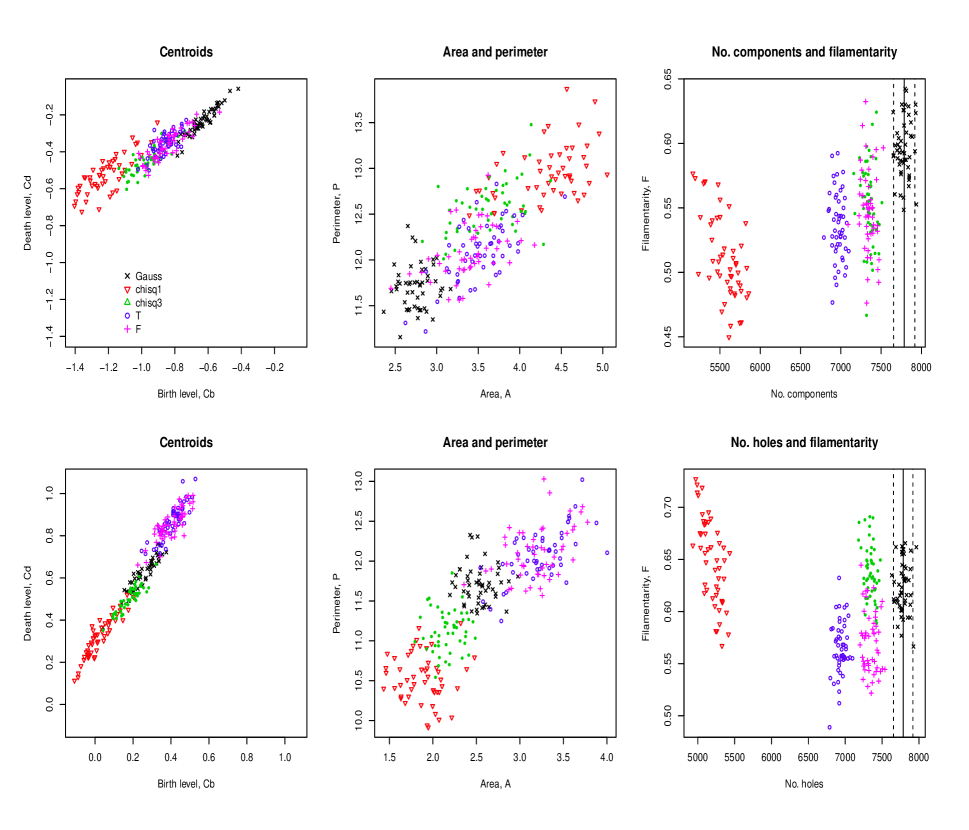
Figure 4: Number of structures and persistence diagram summaries for Models 1–5. Results from 50 realisations of $256\times 256$ fields, with the cross neighbourhood and 90% convex peels. The top row refers to components defined by local minima and the bottom row refers to holes defined by local maxima. The solid vertical lines mark the expected count under a Gaussian random field, with the dashed lines indicating two standard deviations to each side.

5 Testing for differences between fields

We can test an observed field against a Gaussian random field assumption by comparing the observed number of topological features with an interval based on the GRF properties. Figure 4 suggests this may work well. More generally, we might want to distinguish one field from another without assuming a particular distribution. The previous section shows that differences in underlying structure might be detected through topological features but, without theoretical values or an underlying model, we need to develop a data-based approach.

Our proposal is to split the data from each field into subsets which are sufficiently separated for between–subset dependence to be weak, calculate appropriate summary statistics, and then use standard non-parametric statistical tests to compare the summaries from one field with another. Concentrating on $256\times 256$ grids and correlation length around 20 as in the GASS data, we suggest splitting each field into nine $64\times 64$ subsets with buffers of size 32 between them. This gives a reasonable balance between the number of subsets (9) and correlation between them. At the correlation length of 20 that we consider, correlation is 0.20 at the shortest distance between blocks (32), and 0.01 at the separation of block centres (96). Thus although the separate blocks are not independent, association is weak.

Our experience is that the most useful approach is to base tests on two of the summaries: counts $N_{0}$ of components and filamentarity $F$ of persistence diagrams for holes. We suggest a 90% convex peel and use Wilcoxon tests to compare the 9 counts in one field with the 9 in another, and similarly the 9 filamentarities. A Bonferonni correction is used to adjust for the use of two tests. The tests are of course not necessarily independent, and, as stated, we know the subsets are not independent. Nonetheless the simulation results in Table 4 suggest that performance is good. The standard deviation on test size is 0.01 and all estimated test sizes are within noise of the nominal 5%. It is clearly very easy to detect difference between $\chi^{2}_{1}$ fields and any of the others, or between Gauss and $T_{3}$. There is good power for the other comparisons, except for $\chi^{2}_{3}$ against $F_{3,3}$, which are evidently hard to distinguish. Power in this case can be increased by focussing if required only on filamentarity and not using the Bonfernonni correction.

Table 4: Test size and power for nonparametric comparison between pairs of $256\times 256$ random fields. Each value is obtained from 500 simulated pairs, using 5% overall tests after Bonferonni adjustment.

	Gauss	$\chi^{2}_{1}$	$\chi^{2}_{3}$	$T_{3}$	$F_{3,3}$
Gauss	0.050	1.000	0.782	1.000	0.776
$\chi^{2}_{1}$		0.062	1.000	1.000	1.000
$\chi^{2}_{3}$			0.056	0.698	0.160
$T_{3}$				0.038	0.602
$F_{3,3}$					0.040

6 Neutral Hydrogen Distribution in the Milky Way

We now return to the astronomical data, to understand whether the small-scale variation in the regions marked in Figure 1 can be described by simple transfomations of a Gaussian random field, and whether the topologies of this variation can be considered to be the same in each region.

Figure 5 shows, in the top row, 90% convex peels of persistence diagrams for components and holes: it seems that in each case the persistence diagram is more filamentary for Region 3 than the other regions. The bottom row of the figure shows cumulative counts of components and holes as the filtration $\mathcal{F}_{t}$ increases. They include for Region 3 broken lines at plus and minus two estimated standard deviations around the count, obtained from the estimated predictable variation of the counting process (Andersen et al., 1993). We have omitted similar intervals for Regions 1 and 2 as they confuse the plot, but we remark that their widths are very close to those for Region 3. Evidently, the cumulative counts are very similar for Regions 1 and 2 but very different for Region 3. This is confirmed by the final counts, which are given in Table 5. The table also gives the expected counts for a Gaussian random field with Matern correlation matching fits to the data. Clearly, the observed counts are much lower than would be expected for a Gaussian random field, and the difference is stronger for Region 3.

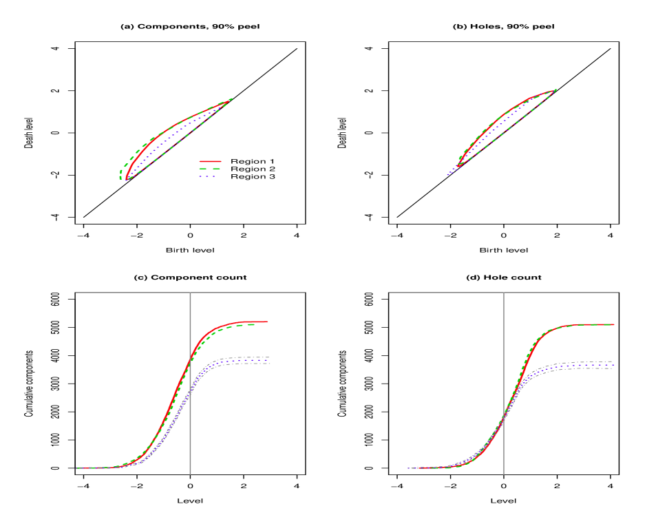
Figure 5: Topological summaries for the GASS data. Regions 1, 2 and 3 as solid, dashed and dotted lines respectively. The broken lines in the bottom row indicate two estimated standard deviations on either side of the Region 3 counts. Standard deviations for the other regions are similar.

Table 6 shows the $p$-values obtained from the data-splitting procedure of Section 5, based on filamentarity and counts. Conclusions are as above, and our answers to both original questions are thus negative. None of the regions has small-scale variation consistent with a simple transformation of a Gaussian random field, and Region 3 has markedly different structure from the other regions.

Table 5: Component and hole counts for the GASS data in the regions shown in Figure 1. The first two numerical columns give estimated parameters for fitted Matern correlation functions. Values in brackets are standard deviations obtained from estimated predictable variation.

	$\nu$	$\eta$	Components	Holes	Gauss expected	Gauss SD
Region 1	0.55	12.98	5201	5100	7896.1	65.9
			(63.1)	(63.6)
Region 2	0.70	13.50	5103	5095	7884.2	65.9
			(62.2)	(66.4)
Region 3	1.08	14.90	3831	3661	7856.1	65.9
			(57.9)	(60.5)

Table 6: $P$-values for comparing the GASS Regions 1–3, based on data splitting into 9 sub-regions and Wilcoxon tests.

	Feature	Filamentarity	Number
Region 1 v Region 2	Components	0.387	0.825
	Holes	0.863	0.825
Region 1 v Region 3	Components	0.077	0.040
	Holes	0.019	0.040
Region 2 v Region 3	Components	0.222	0.027
	Holes	0.031	0.027

Finally for this section we note that the well-known bottleneck distance has no discriminatory power for these data. Table 7 summarises bottleneck distances between all pairs of sub-regions, both within and between regions. Mean intra-region distances can sometimes be larger than mean inter-region values, and any differences in means are small compared to the standard deviations.

Table 7: Mean and standard deviation of bottleneck distances between persistence diagrams of sub-regions. The column $M$ shows the number of pairs for each comparison.

			Components		Holes
Comparison		$M$	Mean	SD	Mean	SD
Region 1	Region 1	36	1.130	0.574	0.542	0.144
Region 1	Region 2	81	1.237	0.528	0.671	0.280
Region 1	Region 3	81	1.314	0.558	0.596	0.131
Region 2	Region 2	36	1.486	0.575	0.799	0.406
Region 2	Region 3	81	1.528	0.620	0.682	0.365
Region 3	Region 3	36	1.287	0.539	0.533	0.171

7 Discussion

Our analyses of the map of interstellar hydrogen (Fig. 1), in terms of the shape of the persistence diagrams and the cumulative counts of topological features, identified Region 3 as being topologically distinct from the other two regions. The regions were deliberately selected without any prior knowledge of the properties of the interstellar medium in these parts of the sky. After carrying out the topological analysis we looked for an astronomical explanation for the distinctive nature of the gas in Region 3 and found that about half of this patch of the sky overlaps a nearby region of recent star formation known as the Orion-Eridanus superbubble (Naranan et al., 1976; Burrows et al., 1993; Pon et al., 2016). Stellar winds and/or supernova explosions have produced a bubble of hot gas, a few hundred light years across, whose boundaries can be traced in many different observational windows, including the H i emission. No structures due to a distinct astronomical object are present in the fields of Regions 1 and 2; in these parts of the sky, the distribution of the H i is most likely the result of pervasive turbulent flows in the interstellar medium. Whilst recognising our identification of the Orion-Eridanus superbubble as retrospective, we speculate this as an explanation for the topological differences between Region 3 and either Regions 1 or 2.

The vast majority of analyses of the GASS or similar astronomical data rely on an assumption of an underlying Gaussian random field, whether for the observational data with or without a simple transformation such as log, or as residuals around some large-scale structure. We have shown that all three of the regions of H i that we examined contain strongly non-Gaussian fields, after trend removal. We suggest that statistical analysis of topological properties is an attractive alternative to existing approaches based on higher-order moments. So far we have considered only two-dimensional data. Extension to three-dimensions may bring further power and is an important problem to address.

References

- (1)
- Adler et al. (2004) Adler, R., Bobrowski, O., Borman, M., Subag, E. & Shmuel Weinberger, S. (2004), Persistent homology for random fields and complexes, in J. Fagerberg, D. C. Mowery & R. R. Nelson, eds, ‘Borrowing Strength: Theory Powering Applications – A Festschrift for Lawrence D Brown’, Institute of Mathematical Statistics, pp. 124–143.
- Adler et al. (2010) Adler, R. J., Bobrowski, O., Borman, M. S., Subag, E. & Weinberger, S. (2010), ‘Persistent homology for random fields and complexes’, Institute of Mathematical Statistics Collections 6, 124–143.
- Adler & Taylor (2011) Adler, R. & Taylor, J. E. (2011), Topological Complexity of Smooth Random Functions: École D’Été Probabilités de Saint-Flour XXXIX-2009 (Lecture Notes in Mathematics), Springer.
- Andersen et al. (1993) Andersen, P., Borgan, O., Gill, R. & Keiding, N. (1993), Statistical Models Based on Counting Processes, Springer-Verlag, New York.
- Arnold (2009) Arnold, B. (2009), ‘Flexible univariate and multivariate models based on hidden truncation’, Journal of Statistical Planning and Inference 139, 3741–3749.
- Azzalini (2005) Azzalini, A. (2005), ‘The skew-normal distribution and related multivariate families (with discussion)’, Scandinavian Journal of Statistics 32, 159–200.
- Bardeen et al. (1986) Bardeen, J., Bond, J., Kaiser, N. & Szalay, A. (1986), ‘The statistics of peaks of Gaussian random fields’, Astrophysical Journal 304, 15–61.
- Barnett (1976) Barnett, V. (1976), ‘The ordering of multivariate data (with discussion)’, Journal of the Royal Statistical Society, Series A 139, 318–355.
- Barrett et al. (2014) Barrett, J., Diggle, P., Henderson, R. & Taylor-Robinson, D. (2014), ‘Joint modelling of repeated measurements and time-to-event outcomes: flexible model specification and exact likelihood inference’, Journal of the Royal Statistical Society, Series B 77, 131–148.
- Bharadwaj et al. (2000) Bharadwaj, S., Sahni, V., Sathyaprakash, B., Shandarin, S. & c Yess, C. (2000), ‘Evidence for filamentarity in the Las Campanas redshift survey’, Astrophysical Journal 528, 21–29.
- Bubenik (2015) Bubenik, P. (2015), ‘Statistical topological data analysis using persistence landscapes’, Journal of Machine Learning Research 16, 77 – 102.
- Burrows et al. (1993) Burrows, D. N., Singh, K. P., Nousek, J. A., Garmire, G. P. & Good, J. (1993), ‘A multiwavelength study of the Eridanus soft X-ray enhancement’, The Astrophysical Journal 406, 97–111.
- Carlsson (2009) Carlsson, G. (2009), ‘Topology and data’, Bulletin of the American Mathematical Society 46, 255–308.
- Chung et al. (2015) Chung, M. K., Hanson, J. L., Ye, J., Davidson, R. J. & Pollak, S. D. (2015), ‘Persistent homology in sparse regression and its application to brain morphometry’, IEEE Transactions on Medical Imaging 34, 1928–1939.
- Chung et al. (2009) Chung, M. K., Singh, V., Kim, P. T., Dalton, K. M. & Davidson, R. J. (2009), ‘Topological characterization of signal in brain images using min-max diagrams’, 12th International Conference on Medical Image Computing and Computer Assisted Intervention. Lecture Notes in Computer Science 5762, 158–166.
- Davis (2008) Davis, B. C. (2008), Medical Image Analysis via Fréchet Means of Diffeomorphisms, PhD Thesis, The University of North Carolina at Chapel Hill.
- Edelsbrunner (2014) Edelsbrunner, H. (2014), A Short Course in Computational Geometry and Topology, Springer.
- Fasy et al. (2014) Fasy, B., Lecci, F., Rinaldo, A., Wasserman, L., Balakrishnan, S. & Aarti Singh, A. (2014), ‘Confidence sets for persistence diagrams’, Annals of Statistics 42, 2301–2339.
- Ferrière (2001) Ferrière, K. (2001), ‘The interstellar environment of our Galaxy’, Reviews of Modern Physics 73, 1031–1066.
- Gay et al. (2010) Gay, C., Pichon, C., Le Borgne, D., Teyssier, R., Sousbie, T. & Devriendt, J. (2010), ‘On the filamentary environment of galaxies’, Monthly Notices of the Royal Astronomical Society 404, 1801–1816.
- Gupta et al. (2004) Gupta, A., Gonzalez-Farias, G. & Dominguez-Molina (2004), ‘A multivariate skew-normal distribution’, Journal of Multivariate Analysis 89, 181–190.
- Kalberla & Kerp (2009) Kalberla, P. & Kerp, J. (2009), ‘The H i distribution of the milky way’, Annual Review of Astronomy and Astrophysics 47, 27–61.
- Kalberla et al. (2010) Kalberla, P., McClure-Griffiths, N., Pisano, D., Calabretta, M., Alyson Ford, H., Lockman, F., Staveley-Smith, L., Kerp, J., Winkel, B., Murphy, T. & Newton-McGee, K. (2010), ‘GASS: the Parkes Galactic all-sky survey II. Stray-radiation correction and second data release’, Astronomy & Astrophysis 521, A17.
- Kramár et al. (2016) Kramár, M., Levanger, R., Tithof, J., Suri, B., Xu, M., Paul, M., Schatz, M. F. & Mischaikow, K. (2016), ‘Analysis of Kolmogorov flow and Rayleigh-Bénard convection using persistent homology’, Physica D Nonlinear Phenomena 334, 82–98.
- Li et al. (2016) Li, G.-X., Urquhart, J. S., Leurini, S., Csengeri, T., Wyrowski, F., Menten, K. M. & Schuller, F. (2016), ‘ATLASGAL: A Galaxy-wide sample of dense filamentary structures’, Astronomy & Astrophysics 591, A5.
- Makarenko et al. (2015) Makarenko, I., Fletcher, A. & Shukurov, A. (2015), ‘3D morphology of a random field from its 2D cross-section’, Monthly Notices of the Royal Astronomical Society 447, L55–L59.
- McClure-Griffiths et al. (2009) McClure-Griffiths, N., Pisano, D., Calabretta, M., Alyson Ford, H., Lockman, F., Staveley-Smith, L., Kalberla, P., Bailin, J., Dedes, L., Janowieck, S., Gibson, B., Murphy, T., Nakanishi, H. & Newton-McGee, K. (2009), ‘GASS: the Parkes Galactic all-sky survey I. Survey description, goals, and initial data release’, The Astrophysical Journal Supplement Series 181, 398–412.
- Naranan et al. (1976) Naranan, S., Shulman, S., Friedman, H. & Fritz, G. (1976), ‘Soft X-ray emission in Eridanus – an old supernova remnant’, The Astrophysical Journal 208, 718–726.
- Pon et al. (2016) Pon, A., Ochsendorf, B. B., Alves, J., Bally, J., Basu, S. & Tielens, A. G. G. M. (2016), ‘Kompaneets model fitting of the Orion-Eridanus superbubble II. Thinking outside of Barnard’s Loop’, The Astrophysical Journal 827, 42.
- Pranav (2015) Pranav, P. (2015), Persistent Holes in the Universe: A Hierarchical Topology of the Cosmic Mass Distribution, PhD thesis, University of Groningen.
- Sousbie (2011) Sousbie, T. (2011), ‘The persistent cosmic web and its filamentary structure I. Theory and implementation’, Monthly Notices of the Royal Astronomical Society 414, 350–383.
- Sousbie et al. (2011) Sousbie, T., Pichon, C. & Kawahara, H. (2011), ‘The persistent cosmic web and its filamentary structure II. Illustrations’, Monthly Notices of the Royal Astronomical Society 414, 384–403.
- Taylor et al. (2007) Taylor, J., Worsley, K. & Gosselin, F. (2007), ‘Maxima of discretely sampled random fields, with an application to ’bubbles”, Biometrika 94, 1–18.
- Yogeshwaran & Adler (2015) Yogeshwaran, D. & Adler, R. J. (2015), ‘On the topology of random complexes built over stationary point processes’, The Annals of Applied Probability 25, 3338–3380.