Sufficient Dimension Reduction via Random-Partitions for Large-$p$-Small-$n$ Problem

Abstract

Sufficient dimension reduction (SDR) is continuing an active research field nowadays for high dimensional data. It aims to estimate the central subspace (CS) without making distributional assumption. To overcome the large-$p$-small-$n$ problem we propose a new approach for SDR. Our method combines the following ideas for high dimensional data analysis: (1) Randomly partition the covariates into subsets and use distance correlation (DC) to construct a sketch of envelope subspace with low dimension. (2) Obtain a sketch of the CS by applying conventional SDR method within the constructed envelope subspace. (3) Repeat the above two steps for a few times and integrate these multiple sketches to form the final estimate of the CS. We name the proposed SDR procedure “integrated random-partition SDR (iRP-SDR)”. Comparing with existing methods, iRP-SDR is less affected by the selection of tuning parameters. Moreover, the estimation procedure of iRP-SDR does not involve the determination of the structural dimension until at the last stage, which makes the method more robust in a high-dimensional setting. Asymptotic properties of iRP-SDR are also established. The advantageous performance of the proposed method is demonstrated via simulation studies and the EEG data analysis.

.

Key words: distance correlation screening; random-partition; random sketch; sliced inverse regression; sufficient dimension reduction; sure screening property.

1 Introduction

In many modern applications, the number of covariates are often too large to provide a parsimonious interpretation or to have insights into the data set. Sufficient dimension reduction (SDR) is thus continuing an active research field nowadays. Let $Y\in\mathbb{R}$ be the response of interest, and let $X=(X_{1},\ldots,X_{p})^{\top}\in\mathbb{R}^{p}$ be the covariates with $E(X)=0$ and ${\rm cov}(X)=\Sigma$. SDR aims to search for a subspace of $\mathbb{R}^{p}$ with a basis $B$ such that

$$Y\;\,\rule[0.0pt]{0.29999pt}{6.69998pt}\rule[0.0pt]{6.49994pt}{0.29999pt}\rule[0.0pt]{0.29999pt}{6.69998pt}\;\,X|B^{\top}X.$$ (1)

The intersections of all such ${\rm span}(B)$ exists under certain conditions (Cook, 1994), which is called the central subspace (CS) for the regression of $Y$ on $X$, and is denoted by $\mathcal{S}_{Y|X}$ with the structural dimension $d={\rm dim}(\mathcal{S}_{Y|X})$. With $B$ being obtained, subsequent analysis can be based on the lower dimensional $(Y,B^{\top}X)$ without losing information. Since the pioneering work of Li (1991), there are many methods developed to estimate $\mathcal{S}_{Y|X}$. One branch of SDR methods can be formulated as the following eigenvalue problem

$$K\beta_{j}=\lambda_{j}\beta_{j}\quad{\rm with}\quad K=\Sigma^{-1}M,\quad j=1,\ldots,p,$$ (2)

where $M$ is a method-specific symmetric matrix. The leading $d$ eigenvectors $\beta_{j}$’s (normalized to $\beta_{j}^{\top}\Sigma\beta_{j}=1$) then provide an estimate of $\mathcal{S}_{Y|X}$. For example, the sliced inverse regression (SIR, Li, 1991) uses $M={\rm cov}\{E(X|Y)\}$ and the sliced average variance estimation (SAVE, Cook and Weisberg, 1991) uses $M=\Sigma^{1/2}E[\{I-{\rm cov}(\Sigma^{-1/2}X|Y)\}^{2}]\Sigma^{1/2}$. We refer the reader to Ma and Zhu (2013) for a review of SDR methods.

Most of the conventional SDR methods become unstable when $p\approx n$ or even fail to apply when $p\gg n$, due to the matrix inversion $\Sigma^{-1}$ in (2). This drawback has limited the usage of many SDR methods when $p$ is large. The problem of inverting $\Sigma$ can be avoided if we can find an envelope subspace $\mathcal{S}_{\rm env}$ such that

$$\mathcal{S}_{Y|X}\subseteq\mathcal{S}_{\rm env},$$ (3)

whose dimension $d_{\rm env}={\rm dim}(\mathcal{S}_{\rm env})$ is relatively smaller than $n$. Let $\mathcal{E}\in\mathbb{R}^{p\times d_{\rm env}}$ be an orthonormal basis of $\mathcal{S}_{\rm env}$, then (3) implies the existence of a matrix $\Gamma\in\mathbb{R}^{d_{\rm env}\times d}$ such that the basis $B$ of $\mathcal{S}_{Y|X}$ can be expressed as

$$B=\mathcal{E}\,\Gamma.$$ (4)

As a result, we have from (1) that $Y\;\,\rule[0.0pt]{0.29999pt}{6.69998pt}\rule[0.0pt]{6.49994pt}{0.29999pt}\rule[0.0pt]{0.29999pt}{6.69998pt}\;\,\mathcal{E}^{\top}X\,|\,\Gamma^{\top}(\mathcal{E}^{\top}X)$, which gives ${\rm span}(\Gamma)=\mathcal{S}_{Y|\mathcal{E}^{\top}X}$. One can then apply any SDR method on $(Y,\mathcal{E}^{\top}X)$ to estimate $\Gamma$ (which is doable since $d_{\rm env}<n$), and transform back to $\mathbb{R}^{p}$ via (4) to estimate $\mathcal{S}_{Y|X}$. For instance, a commonly used strategy to deal with the large-$p$-small-$n$ problem is to apply SDR methods after PCA (PCA-SDR), which is equivalent to construct $\mathcal{E}$ by the leading eigenvectors of $\Sigma$. A similar idea can also be found in the partial inverse regression estimate (PIRE) of Li, Cook and Tsai (2007) and the seeded dimension reduction of Cook, Li and Chiaromonte (2007), where $\mathcal{E}$ is constructed by Krylov sequence.

Different from the above-mentioned methods of PCA-SDR or PIRE, there are another branch of SDR methods, which handle the large-$p$-small-$n$ problem by (i) conducting SDR methods in many lower dimensional subspaces and (ii) integrating SDR results from these sub-problems to obtain a final SDR analysis. Let $\Pi\in\mathbb{R}^{p\times p}$ be a column permutation matrix when multiplied on the right side of a matrix. A size-$r$ subset of $X$ can be written as $\Omega_{r}^{\top}X=:X_{\Omega_{r}}$, where $\Omega_{r}$ is a sampling matrix given by

$$\Omega_{r}^{\top}=\left[I_{r\times r},\,{\bm{0}}_{r\times(p-r)}\right]\Pi.$$ (5)

For SDR on $(Y,X_{\Omega_{r}})$, one only needs to invert $\Omega_{r}^{\top}\Sigma\Omega_{r}$, which is of size $r\times r$. Hilafu (2015) proposed randomized SIR (rSIR) by repeatedly applying SIR on $(Y,X_{\Omega_{r}})$ with multiple randomly generated $\Omega_{r}$’s.

The idea of reducing the problem size by analyzing a random sub-problem has been discussed in the literature of randomized numerical linear algebra and random sketching (see, e.g., Halko, Martinsson and Tropp, 2011; Woodruff, 2014), where a sub-problem provides a sketch of the original problem. The idea of integrating results from multiple sub-problems to improve the accuracy of data analysis can also be found in literature. Chernoff, Lo and Zheng (2009) have demonstrated that influential variables can be effectively identified by repeatedly inspecting the association between $Y$ and $X_{\Omega_{r}}$ for multiple random sampling matrices $\Omega_{r}$’s. Li, Wen and Zhu (2008) proposed to integrate SDR results from multiple random projections of $Y$ to estimate $\mathcal{S}_{Y|X}$ when $Y$ is multivariate. Chen et al. (2016) proposed to integrate multiple random sketches of singular value decomposition. On the other hand, properly using the concept of $\mathcal{S}_{\rm env}$ to confine the inferential target not only can enhance the estimation efficiency, but also can increase the interpretability of analysis results. The aim of this work is to propose a new SDR method, called “integrated random-partition SDR (iRP-SDR)”, to deal with the large-$p$-small-$n$ problem, by utilizing both the ideas of envelope subspace $\mathcal{S}_{\rm env}$ and integration of results from multiple random subsets $X_{\Omega_{r}}$’s.

2 Method: Integrated Random-Partition SDR

The proposed iRP-SDR consists of three major steps:

1. A sketch of the envelope subspace $\mathcal{S}_{\rm env}$ is constructed by a combination of random-partition and distance-correlation screening (see Section 2.1).

2. Conventional SDR method is applied within the sketch of $\mathcal{S}_{\rm env}$ to estimate the kernel matrix $K$ in (2) that avoids inverting $\Sigma$ (see Introduction). Note that the estimate of the kernel matrix depends on the random-partition.

3. Steps 1-2 are repeated a few times and the resulting kernel matrices are integrated. Multiple runs together with an integration to form the final estimate of $\mathcal{S}_{Y|X}$ can reduce the variation due to random-partitions. (see Section 2.2).

2.1 A sketch of $\bm{\mathcal{S}_{\rm env}}$ via random-partition and DC screening

Define the active set of $X$ to be

$$\mathcal{A}=\Big{\{}X_{j}:B(j,k)\neq 0~{}{\rm for~{}some}~{}k\Big{\}}$$ (6)

with $B(j,k)$ being the $(j,k)$-th element of $B$ in (1). The active set $\mathcal{A}$ contains the elements of $X$ that appear in the conditional distribution of $Y$ given $X$. Assume $|\mathcal{A}|<\infty$ and let

$$\mathcal{S}_{\mathcal{A}}={\rm span}\{e_{j}:X_{j}\in\mathcal{A}\},$$ (7)

where $e_{j}\in\mathbb{R}^{p}$ is the vector with 1 in the $j$-th place and 0 elsewhere. Certainly, $\mathcal{S}_{Y|X}\subseteq\mathcal{S}_{\mathcal{A}}$, and any space containing $\mathcal{S}_{\mathcal{A}}$ can serve as an envelope subspace $\mathcal{S}_{\rm env}$ fulfilling (3). The construction of $\mathcal{S}_{\rm env}$ can then be achieved by a proper estimation of $\mathcal{A}$. Fan and Lv (2008) proposed sure independence screening (SIS) to estimate $\mathcal{A}$ by retaining $X_{j}$’s with leading absolute values of Pearson correlation coefficients with $Y$. They showed that SIS possesses the sure screening property under the linear regression model for $Y$ given $X$. The linear regression assumption, however, can be violated in some situations. Moreover, SIS in its nature is a marginal screening method, which ignores the joint effects among $X$. To take the joint effects among $X$ into account, we adopt a screening method based on the distance correlation (DC, Szekely, Rizzo and Bakirov, 2007) to recover $\mathcal{A}$. The squared DC between two random vectors $(v_{1},v_{2})$ is defined to be

$$\omega_{\rm dc}(v_{1},v_{2})=\frac{{\rm dcov}^{2}(v_{1},v_{2})}{{\rm dcov}(v_{1},v_{1}){\rm dcov}(v_{2},v_{2})},$$ (8)

where

$${\rm dcov}^{2}(v_{1},v_{2}) = E\left\{\|v_{1}-\widetilde{v_{1}}\|\cdot\|v_{2}-\widetilde{v_{2}}\|\right\}+E\|v_{1}-\widetilde{v_{1}}\|\cdot E\|v_{2}-\widetilde{v_{2}}\|$$

$$- 2E\left\{E(\|v_{1}-\widetilde{v_{1}}\||v_{1})\cdot E(\|v_{1}-\widetilde{v_{2}}\||v_{2})\right\}$$

and $(\widetilde{v_{1}},\widetilde{v_{2}})$ is a random copy of $(v_{1},v_{2})$. The reasons of using DC are threefold. First, DC measures a general association between two random vectors $(v_{1},v_{2})$, in the sense that $v_{1}\;\,\rule[0.0pt]{0.29999pt}{6.69998pt}\rule[0.0pt]{6.49994pt}{0.29999pt}\rule[0.0pt]{0.29999pt}{6.69998pt}\;\,v_{2}$ if and only if $\omega_{\rm dc}(v_{1},v_{2})=0$. Second, DC is induced from the characteristic function, which is totally model-free. Third, DC can be applied to cases where $v_{1}$ and $v_{2}$ are not of the same dimension, which is able to measure the association between $Y$ and a subset $X_{\Omega_{r}}$.

To recover $\mathcal{A}$ via using $\omega_{\rm dc}$, define a size-$r$ random-partition of $X$ to be a collection of sampling matrices in (5):

$$\mathcal{P}_{r}=\left\{\Omega_{r,k}:k=1,\ldots,\frac{p}{r}\right\}\mbox{~{}such that~{}$\{X_{\Omega_{r,k}}\}_{k=1}^{p/r}$ forms a partition of $X$.}$$ (9)

For simplicity, we assume that $p/r$ is an integer in the rest of discussions. For the case of general $p$, there are $\lfloor p/r\rfloor$ subsets with size $r$ and one subset with size $p-\lfloor p/r\rfloor r$, where $\lfloor\cdot\rfloor$ denotes taking the integer part. For a given $\mathcal{P}_{r}$, we propose to estimate $\mathcal{A}$ by

$$\widehat{\mathcal{A}}_{u}^{(\mathcal{P}_{r})}=\Big{\{}X_{\Omega_{r,k}}:\Omega_{r,k}\in\mathcal{P}_{r},~{}~{}\widehat{\omega}_{\rm dc}(Y,X_{\Omega_{r,k}})\geq c\Big{\}},$$ (10)

where $\widehat{\omega}_{\rm dc}$ is the sample version of $\omega_{\rm dc}$ by replacing expectations with empirical moment estimators, $c$ is a critical value, and $u=u(c)$ denotes the dimension of $\widehat{\mathcal{A}}_{u}^{(\mathcal{P}_{r})}$ under $c$. The selection of critical value will be discussed later. Note that, for $r=1$, $\widehat{\mathcal{A}}_{u}^{(\mathcal{P}_{r})}$ is exactly the marginal screening criterion studied by Li, Zhong and Zhu (2012). They also mentioned the superiority of $\omega_{\rm dc}$ in measuring the association between $Y$ and a subset of $X$, which motivates us to estimate $\mathcal{A}$ by using $\widehat{\mathcal{A}}_{u}^{(\mathcal{P}_{r})}$ with $r\geq 1$. By considering the association between $Y$ and $X_{\Omega_{r,k}}$’s, it not only can take the joint effects among $X$ into account (which is able to integrate weak signals in a subset to a stronger one), but also can reduce the number of units under consideration (which has the potential to increase the power of detecting variables in $\mathcal{A}$). Finally, a basis of $\mathcal{S}_{\rm env}$ is constructed to be the $p\times u$ matrix

$$\widehat{\mathcal{E}}_{u}^{(\mathcal{P}_{r})}=\big{[}\,e_{j}:X_{j}\in\widehat{\mathcal{A}}_{u}^{(\mathcal{P}_{r})}\,\big{]},$$ (11)

which will be used to develop iRP-SDR in the next subsection. Note that $\widehat{\mathcal{E}}_{u}^{(\mathcal{P}_{r})}$, and hence the subsequent analysis, depends on the choices of $\mathcal{P}_{r}$ and the dimension $u$. These issues of stochastic variation in random-partition and hyper-parameters selection will be discussed in Sections 2.2-2.3, respectively.

We close this section by justifying the use of $\widehat{\mathcal{E}}_{u}^{(\mathcal{P}_{r})}$ as a sketch of $\mathcal{S}_{\rm env}$. It mainly relies on the sure screening property of DC screening, which requires that the probability of $\widehat{\mathcal{A}}_{u}^{(\mathcal{P}_{r})}$ containing $\mathcal{A}$ approaches one as $n\to\infty$. Li, Zhong and Zhu (2012) have established the sure screening property for $\widehat{\mathcal{A}}_{u}^{(\mathcal{P}_{r})}$ with $r=1$. Same arguments can be applied to the case of arbitrary $r\geq 1$ under the following assumptions:

• There exists a positive constant $s_{0}$ such that for all $0<s\leq 2s_{0}$,

  $$E\left\{\exp(s\|Y\|^{2})\right\}<\infty~{}~{}{\rm and}~{}~{}\sup_{p}\max_{1\leq j\leq p}E\left\{\exp(s\|X_{j}\|^{2})\right\}<\infty.$$

• The DC value of $Y$ and $X_{\Omega_{r}}$, where $X_{\Omega_{r}}$ contains at least one active variable, is significantly large in the sense that, for some constants $\kappa_{1}>0$ and $0\leq\kappa_{2}<1/2$,

  $$\inf_{\left\{\Omega_{r}:~{}X_{\Omega_{r}}\bigcap\mathcal{A}\neq\emptyset\right\}}\omega_{\rm dc}(Y,X_{\Omega_{r}})\geq 2\kappa_{1}n^{-\kappa_{2}}.$$

Condition (C1) is assumed in Li, Zhong and Zhu (2012), and condition (C2) is modified to adapt to the case of subset size $r\geq 1$. We have the following result.

Theorem 2.1 (sure screening property).

Assume conditions (C1)-(C2), and assume the critical value in $\widehat{\mathcal{A}}_{u}^{(\mathcal{P}_{r})}$ is chosen to be $c=\kappa_{1}n^{-\kappa_{2}}$, where $(\kappa_{1},\kappa_{2})$ are defined in (C2). Then, we have for any $\mathcal{P}_{r}$ that

$$\lim_{n\to\infty}P\left\{\mathcal{A}\subseteq\widehat{\mathcal{A}}_{u}^{(\mathcal{P}_{r})}\big{|}\mathcal{P}_{r}\right\}=1,$$ (12)

where $p$ can take an order $\log p=o\left(n^{(1-2\kappa_{2})/3}\right)$.

Theorem 2.1 implies that $\lim_{n\to\infty}P\{\mathcal{S}_{Y|X}\subseteq{\rm span}(\widehat{\mathcal{E}}_{u}^{(\mathcal{P}_{r})})\big{|}{\mathcal{P}}_{r}\}=1$. It ensures the estimation of $\mathcal{S}_{Y|X}$ can be based on $(Y,\widehat{\mathcal{E}}_{u}^{(\mathcal{P}_{r})\top}X)$. Though the span of $\widehat{\mathcal{E}}_{u}^{(\mathcal{P}_{r})}$ can work as an envelope subspace, its dimension has to be restrained. The dimension of $\widehat{\mathcal{E}}_{u}^{(\mathcal{P}_{r})}$ is given by $u$, which could diverge with $p$ if not properly controlled. To make conventional SDR methods applicable using $(Y,\widehat{\mathcal{E}}_{u}^{(\mathcal{P}_{r})\top}X)$, a simple way is to require $u<\infty$. A sufficient condition to ensure the finiteness of $u$ is to further assume (C3) below.

• The DC value of $Y$ and $X_{\Omega_{r}}$, where $X_{\Omega_{r}}$ does not contain any active variable, is significantly small in the sense that

  $$\sup_{\left\{\Omega_{r}:~{}X_{\Omega_{r}}\bigcap\mathcal{A}=\emptyset\right\}}\omega_{\rm dc}(Y,X_{\Omega_{r}})=o(n^{-\kappa_{2}}),$$

  where $\kappa_{2}$ is defined in (C2).

The following result is essential for Theorem 2.3 below.

Theorem 2.2.

Assume the conditions in Theorem 2.1 and condition (C3). Then, we have for any $\mathcal{P}_{r}$ that

$$\lim_{n\to\infty}P\left\{\widehat{\mathcal{A}}_{u}^{(\mathcal{P}_{r})}=\mathcal{A}^{(\mathcal{P}_{r})}\big{|}\mathcal{P}_{r}\right\}=1,$$

where $\mathcal{A}^{(\mathcal{P}_{r})}=\{X_{\Omega_{r,k}}:\Omega_{r,k}\in\mathcal{P}_{r},X_{\Omega_{r,k}}\bigcap\mathcal{A}\neq\emptyset\}$ with $u_{0}=u_{0}(\mathcal{P}_{r})=|\mathcal{A}^{(\mathcal{P}_{r})}|$ satisfying $d\leq u_{0}<\infty$, and $p$ can take an order $\log p=o\left(n^{(1-2\kappa_{2})/3}\right)$.

2.2 Estimation of $\bm{\mathcal{S}_{Y|X}}$

Below we introduce our iRP-SDR via using $\widehat{\mathcal{E}}_{u}^{(\mathcal{P}_{r})}$ in (11). In the rest of discussions, we use SIR as the core SDR method to explain the details of our proposal. Extensions to other SDR methods based on criterion (2) are straightforward. Given $\mathcal{P}_{r}$, Theorem 2.1 ensures

$$\lim_{n\to\infty}P\left\{B=P_{\widehat{\mathcal{E}}_{u}^{(\mathcal{P}_{r})}}B\big{|}\mathcal{P}_{r}\right\}=1,$$ (13)

where $B$ is a basis of $\mathcal{S}_{Y|X}$, and $P_{M}$ is the orthogonal projection matrix onto ${\rm span}(M)$ for a matrix $M$. It enables the estimation of $\mathcal{S}_{Y|X}$ to be based on $(Y,\widehat{\mathcal{E}}_{u}^{(\mathcal{P}_{r})\top}X)$, which avoids inverting $\Sigma$. In particular, let $\widehat{\gamma}_{j}^{(\mathcal{P}_{r})}$ and $\widehat{\lambda}_{j}^{(\mathcal{P}_{r})}$ be the $j$-th eigenvector and eigenvalue obtained from applying SIR on $(Y,\widehat{\mathcal{E}}_{u}^{(\mathcal{P}_{r})\top}X)$, $j=1,\ldots,u$. Let also

$$\widehat{\beta}_{j}^{(\mathcal{P}_{r})}=\widehat{\mathcal{E}}_{u}^{(\mathcal{P}_{r})}\,\widehat{\gamma}_{j}^{(\mathcal{P}_{r})},\quad j=1,\ldots,u,$$ (14)

which transforms $\widehat{\gamma}_{j}^{(\mathcal{P}_{r})}$ back to $\mathbb{R}^{p}$ via (4). Since the leading eigenvectors $\widehat{\gamma}_{j}^{(\mathcal{P}_{r})}$’s provide an estimate of $\mathcal{S}_{Y|\widehat{\mathcal{E}}_{u}^{(\mathcal{P}_{r})\top}X}$, it implies from (13) that $\widehat{\beta}_{j}^{(\mathcal{P}_{r})}$’s provide an estimate of $\mathcal{S}_{Y|X}$. The projection matrix (with respect to the $\Sigma$-inner product) associated with $\widehat{\beta}_{j}^{(\mathcal{P}_{r})}$ is given by $\widehat{\beta}_{j}^{(\mathcal{P}_{r})}\big{\{}\widehat{\beta}_{j}^{(\mathcal{P}_{r})\top}\Sigma\widehat{\beta}_{j}^{(\mathcal{P}_{r})}\big{\}}^{-1}\widehat{\beta}_{j}^{(\mathcal{P}_{r})\top}\Sigma$, which is estimated by $\widehat{\beta}_{j}^{(\mathcal{P}_{r})}\widehat{\beta}_{j}^{(\mathcal{P}_{r})\top}\widehat{\Sigma}$. The projection matrix enables us to summarize the $\mathcal{P}_{r}$-analysis via the kernel matrix

$$\widehat{K}_{u}^{(\mathcal{P}_{r})}=\sum_{j=1}^{u}\widehat{\lambda}_{j}^{(\mathcal{P}_{r})}\,\widehat{\beta}_{j}^{(\mathcal{P}_{r})}\beta_{j}^{(\mathcal{P}_{r}){\top}}{\widehat{\Sigma}},$$ (15)

where the subscript $u$ indicates that the construction of $\widehat{K}_{u}^{(\mathcal{P}_{r})}$ is based on the $u$-dimensional $\widehat{\mathcal{E}}_{u}^{(\mathcal{P}_{r})}$. One can treat $\widehat{K}_{u}^{(\mathcal{P}_{r})}$ as an estimate of the SIR kernel matrix pre-multiplied by $\Sigma^{-1}$, which has $\widehat{\beta}_{j}^{(\mathcal{P}_{r})}$ as its eigenvector with eigenvalue $\widehat{\lambda}_{j}^{(\mathcal{P}_{r})}$. See Remark 2.4 for details.

Although the kernel matrix $\widehat{K}_{u}^{(\mathcal{P}_{r})}$ provides a basis to estimate $\mathcal{S}_{Y|X}$ without inverting $\Sigma$, it only produces a sketch estimate with less precision. Moreover, the analysis result will depend on the choice of the random-partition $\mathcal{P}_{r}$. There generally exists no prior knowledge about how $X$ should be partitioned in the SDR problem. A natural strategy is to consider the expected value of $\widehat{K}_{u}^{(\mathcal{P}_{r})}$ with respect to the uniform distribution for $\mathcal{P}_{r}$. An integrated kernel matrix is proposed to be

$$\widehat{K}_{u,r}=E_{\mathcal{P}_{r}}[\widehat{K}_{u}^{(\mathcal{P}_{r})}]=\frac{1}{N_{r}}\sum_{l=1}^{N_{r}}\widehat{K}_{u}^{(\mathcal{P}_{r,l})},$$ (16)

where $\{\mathcal{P}_{r,l}:l=1,\ldots,N_{r}\}$ denotes the collection of all possible size-$r$ random-partitions of $X$. Plugging in $K=\widehat{K}_{u,r}$ to (2), a basis of $\mathcal{S}_{Y|X}$ can be estimated by the leading $d$ eigenvectors of $\widehat{K}_{u,r}$. The consistency of $\widehat{K}_{u,r}$ is stated below.

Theorem 2.3 (consistency).

Assume conditions (C1)-(C3), and assume that the critical value in $\widehat{\mathcal{A}}_{u}^{(\mathcal{P}_{r})}$ is chosen to be $c=\kappa_{1}n^{-\kappa_{2}}$, where $(\kappa_{1},\kappa_{2})$ are defined in (C2). Assume also that SIR based on $(Y,X_{\Omega})$ is a consistent estimator of $\mathcal{S}_{Y|X_{\Omega}}$ for any sampling matrix $\Omega$ satisfying $\mathcal{S}_{Y|X}\subseteq{\rm span}(\Omega)$. Then, as $n\to\infty$, we have $\|P_{\widehat{K}_{u,r}}-P_{B}\|_{F}\to 0$ in probability, where $\|\,\cdot\,\|_{F}$ stands for matrix Frobenius norm.

Remark 2.4.

The kernel matrix $K$ in criterion (2) is symmetric in the metric of $\Sigma$, i.e., $\Sigma K$ is symmetric (Tyler, 1981). The spectral theory then implies that $K=\sum_{j}\lambda_{j}\beta_{j}\beta_{j}^{\top}\Sigma$ with $(\beta_{j},\lambda_{j})$ being its eigenvector and eigenvalue. This representation motivates the construction of $\widehat{K}_{u}^{(\mathcal{P}_{r})}$ in (15). In this viewpoint, $\widehat{K}_{u}^{(\mathcal{P}_{r})}$ can be treated as a sketch estimate of the SIR kernel matrix $\Sigma^{-1}{\rm cov}(E(X|Y))$ but without the need of inverting $\Sigma$.

2.3 Tuning parameters and structural dimension

There are two tuning parameters involved in iRP-SDR, including the critical value $c$ for constructing $\widehat{\mathcal{E}}_{u}^{(\cdot)}$ and the subset size $r$ of the random-partition $\mathcal{P}_{r}$. Note that choosing $c$ is equivalent to choosing the envelope dimension $u$. We provide two simple settings, $\widehat{K}_{u}$ in (17) and $\widehat{K}$ in (18) below, for the tuning parameters $(u,r)$.

We first deal with the selection of $r$ with a given $u$. The value of $r$ determines the subset size of the random-partition used to construct $\widehat{\mathcal{E}}_{u}^{(\cdot)}$. A larger $r$ makes $\omega_{\rm dc}(Y,X_{\Omega_{r,k}})$ more capable to reflect the joint effects among $X$, but at the cost of being less efficient in estimating $\omega_{\rm dc}(Y,X_{\Omega_{r,k}})$ with limited sample size $n$. There generally exists no prior knowledge of an ideal partition size, and a natural strategy is to consider all possible choices of $r$. Let $\mathcal{R}_{u}$ be the candidate set of choices of $r$, which consists of the unique elements of $\{\lfloor\frac{u}{s}\rfloor:s=1,\ldots,u\}$. E.g., for $u=6$, we have $\mathcal{R}_{u}=\{1,2,3,6\}$. For any $r\in\mathcal{R}_{u}$, we include in $\widehat{\mathcal{A}}_{u}^{(\mathcal{P}_{r})}$ those subsets $X_{\Omega_{r,k}}$’s with the largest $u/r$ values of $\widehat{\omega}_{\rm dc}(Y,X_{\Omega_{r,k}})$’s. When $u/r$ is not an integer, we select $\lfloor u/r\rfloor$ subsets. This procedure gives $|\widehat{\mathcal{A}}_{u}^{(\mathcal{P}_{r})}|=r\lfloor u/r\rfloor\leq u$. The integrated kernel matrix over $r\in\mathcal{R}_{u}$ is given by

$$\widehat{K}_{u}=\sum_{r\in\mathcal{R}_{u}}\widehat{K}_{u,r}.$$ (17)

An estimate of $\mathcal{S}_{Y|X}$ is proposed to be $\widehat{B}_{u}$, the leading $d$ eigenvectors of $\widehat{K}_{u}$. This kernel matrix $\widehat{K}_{u}$ simplifies the tuning parameter to just one number $u$, the dimension of the envelope $\widehat{\mathcal{E}}_{u}^{(\cdot)}$. Note that most of the SDR methods for large-$p$-small-$n$ problem eventually face the issue of choosing a tuning parameter of certain dimensionality. For example, PCA-SDR needs to determine the number of the leading eigenvectors of $\widehat{\Sigma}$, PIRE needs to determine the dimension of the Krylov sequence, and both rSIR and seq-SDR need to determine the subset size to reduce the dimension of $X$ sequentially. While Cook, Li and Chiaromonte (2007) proposed a testing method to determine the dimension of the Krylov sequence, there is no theoretical support developed concerning this issue in rSIR and seq-SDR. Considering the fact that $u$ is the reduced model size such that SIR can be properly implemented using $(Y,\widehat{\mathcal{E}}_{u}^{(\mathcal{P}_{r})\top}X)$ with sample size $n$, we can use $u=\lfloor na\rfloor$ for some $a\in(0,1)$. Of course the selection of $u$ will affect the performance of iRP-SDR. The optimal selection of $u$ depends on the underlying data generating distribution, and is beyond the scope of this work. Alternatively, we can make the inference procedure less affected by the selection of $u$, by using an ensemble approach with the integrated kernel matrix

$$\widehat{K}=\sum_{u\in\mathcal{U}}\frac{1}{m_{u}}\widehat{K}_{u},$$ (18)

where $\mathcal{U}$ is a pre-determined set of possible values of $u$, and $m_{u}$ is the sum of eigenvalues of $\widehat{K}_{u}$. Dividing $m_{u}$ makes the kernel matrices $\frac{1}{m_{u}}\widehat{K}_{u}$’s from different envelope sizes comparable. Finally, an ensemble estimate of $\mathcal{S}_{Y|X}$ is proposed to be $\widehat{B}$, the leading $d$ eigenvectors of $\widehat{K}$. Note that both $\widehat{K}_{u}$ and $\widehat{K}$ are finite sums of $\widehat{K}_{u,r}$’s. The consistency of $\widehat{B}_{u}$ or $\widehat{B}$ in estimating $\mathcal{S}_{Y|X}$ is thus a direct consequence of Theorem 2.3.

The structural dimension $d$ can be determined by existing methods based on the kernel matrix $\widehat{K}_{u}$ or $\widehat{K}$. We suggest using the Bayesian information criterion (BIC) of Zhu et al. (2010) to select $d$ by

$$\widehat{d}=\mathop{\rm argmin}_{k=1,\ldots,p}\left\{\frac{n\sum_{j=1}^{k}\{\ln(\ell_{j}+1)-\ell_{j}\}}{2\sum_{j=1}^{p}\{\ln(\ell_{j}+1)-\ell_{j}\}}-2C_{n}\frac{k(k-1)}{2p}\right\},$$ (19)

where $\ell_{j}$’s represent the eigenvalues of $\widehat{K}_{u}$ or $\widehat{K}$, and $C_{n}$ is the user-defined penalty. The consistency of $\widehat{d}$ follows from the same argument of Zhu et al. (2010) and the consistency of $\widehat{K}_{u}$ or $\widehat{K}$, provided that $C_{n}/n\to 0$ and $C_{n}\to\infty$ as $n\to\infty$.

3 Characteristics of iRP-SDR

The proposed iRP-SDR possesses some characteristics that make it more adaptive and stable in estimating $\mathcal{S}_{Y|X}$ under the high-dimensional setting.

1. iRP-SDR is adaptive to various situations. The success of iRP-SDR in recovering $\mathcal{S}_{Y|X}$ mainly relies on the sure screening property (12) of a ranking and screening method, which is satisfied under the conditions (C1)-(C2).

2. iRP-SDR does not involve the estimation of the structural dimension $d$ until at the final stage. Most of SDR methods for large-$p$-small-$n$ problem require determining the structural dimension during the estimation process, which may suffer the problem of instability. iRP-SDR performs as the conventional SDR methods that determines $d$ from the integrated kernel matrix $\widehat{K}_{u}$ or $\widehat{K}$.

3. iRP-SDR is easy to implement. Besides the tuning parameters for the core SDR method (e.g., the slicing number of SIR), iRP-SDR only depends on the envelope size $u$. iRP-SDR is also able to combine with any SDR method with the estimation criterion (2). Moreover, iRP-SDR has the potential to adapt to extremely large data set, since the calculations of different $\widehat{K}_{u}^{(\mathcal{P}_{r,l})}$’s can be in parallel.

4 Numerical Studies

4.1 Simulation settings

Let $\varepsilon\sim N(0,1)$ be the error term. We consider the following models from the literature.

1. (Li, Cook and Tsai, 2007). Set $(n,p)=(100,300)$. Each element of $X$ is from $U(0,1)$, and $Y=\log(|B^{\top}X-4|)+\sigma_{0}\varepsilon$ with $B=(-0.5,1,0.5,1,-1,-0.8,0.8,1,0.5,0.75,\textbf{0}_{p-10}^{\top})^{\top}$.

2. (Yin and Hilafu, 2015). Set $(n,p)=(200,1000)$. Let $X\sim N(0,\Sigma)$ with the $(j_{1},j_{2})$-th element of $\Sigma$ being $0.5^{|j_{1}-j_{2}|}$ and $Y=1+\exp(B^{\top}X)+\varepsilon$ with $B=(\textbf{0}_{500}^{\top},1,1,1,1,\textbf{0}_{p-504}^{\top})^{\top}$.

3. (Hilafu and Yin, 2016). Set $(n,p)=(100,500)$. Let $X\sim N(0,0.5I_{p}+0.5\textbf{1}_{p}\textbf{1}_{p}^{\top})$ and $Y=0.5\exp(0.75\cdot B^{\top}X)\varepsilon$ with $B=(-0.5,1,0.5,1,-1,-0.8,0.8,1,0.5,0.75,\textbf{0}_{p-10}^{\top})^{\top}$.

4. (Hilafu and Yin, 2016). Set $(n,p)=(100,500)$. Let $Y\sim U(0,1)$ and $X=\beta_{1}Y+\beta_{2}Y^{2}+0.5E$ with $E\sim N(0,0.5I_{p}+0.5\textbf{1}_{p}\textbf{1}_{p}^{\top})$, $\beta_{1}=(0.5,0.75,\textbf{0}_{p-2}^{\top})^{\top}$, and $\beta_{2}=(0,0,0.75,0.5,\textbf{0}_{p-4}^{\top})^{\top}$. It gives $B=(0.5I_{p}+0.5\textbf{1}_{p}\textbf{1}_{p}^{\top})^{-1}[\beta_{1},\beta_{2}]$.

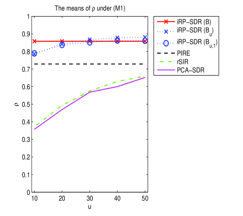
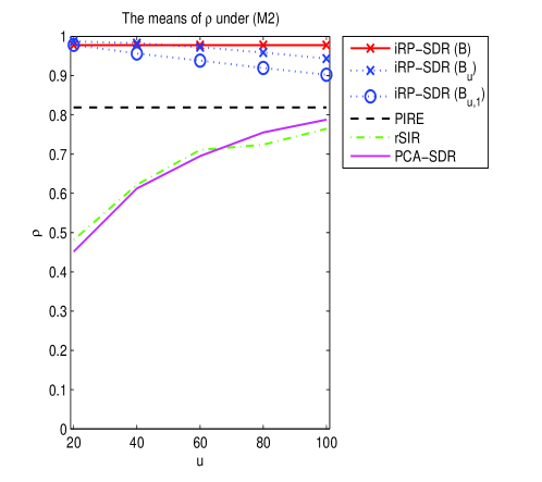
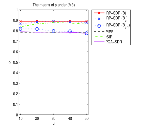
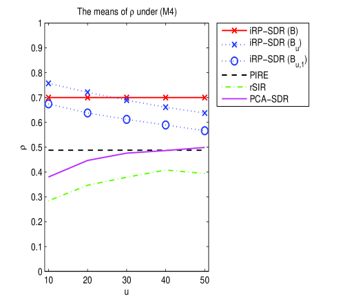
Figure 1: The means of $\rho$ at different envelope sizes $u$ under models (M1)-(M4).

Let $\mathcal{U}=\{0.1n,0.2n,\ldots,0.5n\}$ be the candidate set of the envelope dimension $u$. We implement $\widehat{B}_{u}$ of iRP-SDR with $u\in\mathcal{U}$, PIRE with the Krylov sequence dimension $u\in\mathcal{U}$, rSIR with the subset size $u\in\mathcal{U}$, and PCA-SDR with $u\in\mathcal{U}$ leading eigenvectors of $\widehat{\Sigma}$, so that all methods use the same envelope dimension $u$. Following Hilafu and Yin (2016), the slicing number of SIR used in all methods is set to 5. The mean absolute value of the trace correlation $\rho=\rho(\widetilde{B}^{\top}X,B^{\top}X)$ is reported to summarize the performance of an estimator $\widetilde{B}$, where $\rho(v_{1},v_{2})=\sqrt{{\rm trace}(V)/{\rm dim}(V)}$ with $V=\Sigma_{v_{2}}^{-1/2}\Sigma_{v_{1}v_{2}}^{\top}\Sigma_{v_{1}}^{-1}\Sigma_{v_{1}v_{2}}\Sigma_{v_{2}}^{-1/2}$, $\Sigma_{v_{1}}={\rm cov}(v_{1})$, $\Sigma_{v_{2}}={\rm cov}(v_{2})$, and $\Sigma_{v_{1}v_{2}}={\rm cov}(v_{1},v_{2})$, and $\rho=1$ indicates that ${\rm span}(\widetilde{B})={\rm span}(B)$. Simulation results of $\rho$ with 100 replicates are placed in Figure 1. We remind the reader that all methods considered in our simulation studies use SIR as the core SDR method. The simulation results then directly reflect the capability of each method in dealing with the large-$p$-small-$n$ problem, while controlling the capability of SIR in estimating $\mathcal{S}_{Y|X}$.

4.2 Simulation results: comparison with the case of $r=1$

A critical step of iRP-SDR is the construction of $\mathcal{S}_{\rm env}$ via random-partitions of $X$ (with subset size $r$) having leading DC values with $Y$. Recall that using $r>1$ ensures iRP-SDR to take the joint effects among $X$ into account, while $r=1$ corresponds to using marginal DC values $\widehat{\omega}_{\rm dc}(Y,X_{j})$’s to construct $\mathcal{S}_{\rm env}$, which totally ignores the joint effects among $X$. The first simulation study aims to evaluate the gain from using $r>1$ to the estimation of $\mathcal{S}_{Y|X}$. To see this, we also report in Figure 1 the simulation results from the kernel matrix $\widehat{K}_{u,r}$ in (16) with $r=1$ (denoted by $\widehat{B}_{u,1}$). Comparing $\widehat{B}_{u}$ (from the integrated kernel matrix $\widehat{K}_{u}$) with $\widehat{B}_{u,1}$, it can be seen that $\widehat{B}_{u}$ outperforms $\widehat{B}_{u,1}$ uniformly under all models, especially for the cases of (M2)-(M4). Note that in (M1), the elements of $X$ are independently generated, under which we gain less from considering the joint effects among $X$, and $\widehat{B}_{u}$ and $\widehat{B}_{u,1}$ are detected to have similar performances. As to (M2)-(M4), $X$ are correlated and the gain from grouping $X$ becomes obvious. Our simulation study shows the merits of using $r>1$, and that $\widehat{B}_{u}$ outperforms $\widehat{B}_{u,1}$ even when the covariates are mutually independent.

4.3 Simulation results: comparison with other methods

We first compare $\widehat{B}_{u}$ of iRP-SDR with the $\mathcal{S}_{\rm env}$-based SDR methods: PIRE and PCA-SDR. It can be seen that $\widehat{B}_{u}$ outperforms PIRE and PCA-SDR under all models. The performance of PCA-SDR can be heavily affected by the choice of $u$, especially for the cases of (M1)-(M2). Recall that PCA-SDR assumes that $\mathcal{S}_{Y|X}$ is spanned by the leading eigenvectors of $\Sigma$. This condition can be satisfied for a large $u$ only. A large $u$, however, can also include in $\mathcal{S}_{\rm env}$ more irrelevant directions outside $\mathcal{S}_{Y|X}$, which further decreases the estimation efficiency. PIRE also requires $\mathcal{S}_{Y|X}$ to be spanned by the leading directions of Krylov sequence. Unlike PCA-SDR, the construction of Krylov sequence in PIRE uses the information of $Y$. However, our simulation results indicate a limitation of the Krylov sequence in capturing $\mathcal{S}_{Y|X}$, where PIRE cannot have better performance than $\widehat{B}_{u}$ for all $u$. Recall the validity of iRP-SDR merely relies on the sure screening property, which is not related to any specific structure of $\mathcal{S}_{Y|X}$. iRP-SDR is thus expected to be more adaptive to various situations. Another reason for the unsatisfactory performance of PIRE and PCA-SDR is that their construction of $\mathcal{S}_{\rm env}$ involves a $p$-dimensional eigen-decomposition (i.e., eigenvectors of $\widehat{\Sigma}$ in PCA-SDR, and $\nu$ in PIRE) with $n\ll p$. On the other hand, iRP-SDR constructs $\mathcal{S}_{\rm env}$ via random-partitions of $X$, each with subset size $r$ only. Considering the limited sample size, it is also reasonable to expect an efficiency gain of iRP-SDR over PIRE and PCA-SDR. We next compare $\widehat{B}_{u}$ with the subset-based SDR methods: rSIR. Although rSIR has comparable performances with $\widehat{B}_{u}$ under (M3), it fails to identify $\mathcal{S}_{Y|X}$ under (M1), (M2), and (M4). It indicates that simply using random subset of $X$ cannot provide a consistent estimate of $\mathcal{S}_{Y|X}$, and the naive integration method is not suitable to integrate multiple results, either.

The simulation results of the ensemble approach $\widehat{B}$ over $u\in\mathcal{U}$ are also reported in Figure 1. It can be seen that $\widehat{B}$ always produces comparable results with $\widehat{B}_{u}$, and also dominates other competitors. It implies that $\widehat{B}$ is less affected by the selection of the envelope size and can achieve satisfactory results. Thus, the ensemble $\widehat{B}$ is suggested in practice.

5 The EEG Data

The EEG data set (downloaded from the UCI machine learning repository) consists of $n=122$ samples, each with a 256$\times$64 matrix $X_{0}$ and a binary alcoholic status $Y$. The $(j,k)$-th element of $X_{0}$ represents the voltage value of the $k$-th probe measured at the $j$-th time point. It is of interest to construct a prediction model based on the voltage value for the alcoholic status. In our analysis, we preprocess the data matrix $X_{0}$ to form $\bar{X}_{0}$, where $\bar{X}_{0}(j,k)={\rm median}\{X_{0}(\ell,k):32(j-1)+1\leq\ell\leq 32j\}$, $k=1,\ldots,64$. That is, $\bar{X}_{0}$ is obtained from summarizing $X_{0}$ over $32$ time points, while keeping the data structure of 64 channels. It gives the dimension of $\bar{X}_{0}$ to be $8\times 64$, where the $(j,k)$-th element of $\bar{X}_{0}$ represents the median voltage value of the $k$-th probe over the time period $[32(j-1)+1,32j]$. We then use the data $(Y,X)$ to enter our analysis, where $X={\rm vec}(\bar{X}_{0})$ has dimension $p=8\times 64=512$.

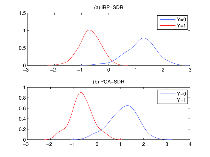
Figure 2: The density estimates for two groups of subjects in the EEG data analysis: (a) iRP-SDR ($\widehat{B}_{50}$); and (b) PCA-SDR ($u=50$).

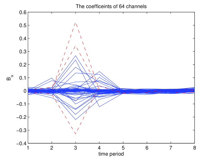
Figure 3: The coefficients $\widehat{B}_{50}$ in the EEG data analysis, where each of the 64 curves represents the coefficients of a channel at 8 time periods. The dotted curves represent the channels O2 ($k=30$), P2 ($k=60$), and P4 ($k=24$) that have absolute values of $\widehat{B}_{50}$ larger than 0.3 at the 3rd time period, i.e., $|\widehat{B}_{50}(3,k)|>0.3$.

The analysis result of iRP-SDR ($\widehat{B}_{u}$) with $u=50$ and $d=1$ (since SIR can identify a single direction for binary $Y$) is placed in Figure 2 (a), which reports the density estimates of $\widehat{B}_{50}^{\top}X|Y=y$, $y=0,1$. One can see that the two density estimates from iRP-SDR are well separated, which indicates a clear separation on the means of the EEG signals for two types of subjects. The analysis result of PCA-SDR (with $u=50$) is reported in Figure 2 (b) for comparison. Although the density estimates from PCA-SDR also show a clear separation of locations, the overlapping area is detected to be larger than that from iRP-SDR. It demonstrates the capability of iRP-SDR to extract more information from high-dimensional data. The coefficients $\widehat{B}_{50}$ (from using component-wisely standardized $X$) from iRP-SDR are reported in Figure 3, where each of the 64 curves represents the coefficients of a channel at 8 time periods. It is observed that the curves tend to have a large absolute coefficients at the 3rd time period, but have nearly zero effects after the 4th time period. It indicates an early reaction of the brain to the stimulus for alcoholic patients. The dotted curves represent the channels having absolute values of $\widehat{B}_{50}$ larger than 0.3 at the 3rd time period (i.e., $|\widehat{B}_{50}(3,k)|>0.3$), including O2 ($k=30$), P2 ($k=60$), and P4 ($k=24$) that locate nearly on the right brain. It suggests that the areas of Parietal and Occipital on the right brain control the reaction to alcoholic stimulus.

To further demonstrate the performance of iRP-SDR, we construct a prediction model based on $(Y,\widehat{B}_{u}^{\top}X)$ by linear discriminant analysis (LDA), and the leave-one-out classification accuracy (CA) from the whole procedure (i.e., SDR followed by LDA prediction) with different $u$ values are reported in Table 1. One can see that iRP-SDR produces higher CA values than PCA-SDR for every envelope size $u$. Moreover, the performances of iRP-SDR are quite stable for different choices of $u$. Our EEG data analysis again demonstrates the superiority of iRP-SDR in estimating $\mathcal{S}_{Y|X}$ when $n\ll p$.

6 Discussion

In this paper, we propose a novel iRP-SDR method for large-$p$-small-$n$ SDR problem. The superiority of iRP-SDR comes from the combination of $\mathcal{S}_{\rm env}$ and random-partition as well as integration of results from multiple random-partitions. The construction of $\mathcal{S}_{\rm env}$ ensures the consistency of iRP-SDR in identifying $\mathcal{S}_{Y|X}$, while the random-partition makes iRP-SDR to take the joint effects among $X$ into account. iRP-SDR is also easy to implement with a single tuning parameter of the envelope size $u$, and the computation of $\widehat{K}_{u}^{(\mathcal{P}_{r,l})}$ can be put in parallel. The superiority of iRP-SDR is demonstrated via numerical studies and the EEG data set.

In iRP-SDR, we use DC as the ranking method to construct $\mathcal{S}_{\rm env}$. There exist other ranking methods that are able to measure the association between $Y$ and a subset of $X$. We note that any ranking method satisfying the sure screening property (12) can be used in iRP-SDR. Another feature that could affect the performance of iRP-SDR is the integration method for multiple results. In this paper, we use sample mean to form the integrated kernel matrix (16) for simplicity. It is of interest to study the effects of different ranking and integration methods on the performance of iRP-SDR.

References

Chen, T. L., Chang, D., Huang, S. Y., Chen, H., Chang, C. and Wang, W. (2016). Integrating multiple random sketches for singular value decomposition. arXiv:1608.08285.

Chernoff, H., Lo, S. H., and Zheng, T. (2009). Discovering influential variables: a method of partitions. The Annals of Applied Statistics, 1335-1369.

Cook, R. D. (1994). On the interpretation of regression plots. Journal of the American Statistical Association, 89(425), 177-189.

Cook, R. D., Li, B., and Chiaromonte, F. (2007). Dimension reduction in regression without matrix inversion. Biometrika, 94(3), 569-584.

Cook, R. D. and Weisberg, S. (1991). Discussion of “Sliced inverse regression for dimension reduction”. Journal of the American Statistical Association, 86, 328-332.

Fan, J. and Lv, J. (2008). Sure independence screening for ultrahigh dimensional feature space. Journal of the Royal Statistical Society: Series B, 70, 849-911.

Halko, N., Martinsson, P. G. and Tropp, J. A. (2011). Finding structure with randomness: probabilistic algorithms for constructing approximate matrix decompositions. SIAM Review, 53(2), 217-288.

Hilafu, H. (2015). Random Sliced Inverse Regression. Communications in Statistics-Simulation and Computation, accepted.

Hilafu, H. and Yin, X. (2017). Sufficient dimension reduction and variable selection for large-p-small-n data with highly correlated predictors. Journal of Computational and Graphical Statistics, 26, 26-34.

Lee, M., Shen, H., Huang, J. Z., and Marron, J. S. (2010). Biclustering via sparse singular value decomposition. Biometrics, 66, 1087-1095.

Li, B., Wen, S. and Zhu, L. (2008). On a projective resampling method for dimension reduction with multivariate responses. Journal of the American Statistical Association, 103(483), 1177-1186.

Li, K. C. (1991). Sliced inverse regression for dimension reduction. Journal of the American Statistical Association, 86, 316-327.

Li, L., Cook, R. D., and Tsai, C. L. (2007). Partial inverse regression. Biometrika, 94(3), 615-625.

Li, R., Zhong, W., and Zhu, L. (2012). Feature screening via distance correlation learning. Journal of the American Statistical Association, 107(499), 1129-1139.

Ma, Y. and Zhu, L. (2013). A review on dimension reduction. International Statistical Review, 81, 134-150.

Szekely, G. J., Rizzo, M. L., and Bakirov, N. K. (2007). Measuring and testing dependence by correlation of distances. The Annals of Statistics, 35, 2769-2794.

Tyler, D. E. (1981). Asymptotic inference for eigenvectors. The Annals of Statistics, 9, 725-736.

Woodruff, D. P. (2014). Sketching as a tool for numerical linear algebra. Foundations and Trends in Theoretical Computer Science, 10(1-2), 1-157.

Yin, X. and Hilafu, H. (2015). Sequential sufficient dimension reduction for large p, small n problems. Journal of the Royal Statistical Society: Series B, 77, 879-892.

Zhu, L., Miao, B., and Peng, H. (2006). On sliced inverse regression with high-dimensional covariates. Journal of the American Statistical Association, 101, 630-643.

Zhu, L. P., Li, L., Li, R., and Zhu, L. X. (2011). Model-free feature screening for ultrahigh-dimensional data. Journal of the American Statistical Association, 106, 1464-1475.

Zhu, L. P., Zhu, L. X., Ferre, L., and Wang, T. (2010). Sufficient dimension reduction through discretization-expectation estimation. Biometrika 97, 295-304.

Table 1: The leave-one-out classification accuracies of iRP-SDR ($\widehat{B}_{u}$) and PCA-SDR at different envelope sizes $u$ in the EEG data analysis.

$u$	iRP-SDR	PCA-SDR
30	0.803	0.721
35	0.844	0.787
40	0.828	0.820
45	0.853	0.795
50	0.844	0.779
55	0.853	0.771
60	0.820	0.803