The supernova-regulated ISM. IV. A comparison of simulated polarization with Planck observations

Abstract

Context. The efforts for comparing dust polarization measurements with synthetic observations from MHD models have previously concentrated on the scale of molecular clouds.

Aims. Here we extend the model comparisons to kiloparsec scales, taking into account hot shocked gas generated by supernovae, and a non-uniform dynamo-generated magnetic field at both large and small scales down to 4 pc spatial resolution.

Methods. Radiative transfer calculations are used to model dust emission and polarization on the top of MHD simulations. We compute synthetic maps of column density $N_{\mathrm{H}}$, polarization fraction $p$, and polarization angle dispersion $\mathcal{S}$, and study their dependencies on the important properties of the MHD simulations. These include the large-scale magnetic field and its orientation, the small-scale magnetic field, and supernova-driven shocks.

Results. Similar filament-like structures of $\mathcal{S}$ as seen in the Planck all-sky maps are visible in our synthetic results, although the smallest scale structures are absent from our maps. Supernova-driven shock fronts and $\mathcal{S}$ do not show significant correlation. Instead, $\mathcal{S}$ can clearly be attributed to the distribution of the small-scale magnetic field. We also find that the large-scale magnetic field influences the polarization properties, such that, for a given strength of magnetic fluctuation, a strong plane-of-the-sky mean field weakens the observed $\mathcal{S}$, while strengthening $p$. The anticorrelation of $p$ and $\mathcal{S}$, and decreasing $p$ as a function of $N_{\mathrm{H}}$ are consistent across all synthetic observations. The magnetic fluctuations follow an exponential distribution, rather than Gaussian, characteristic of flows with intermittent repetitive shocks.

Conclusions. The observed polarization properties and column densities are sensitive to the line of sight distance over which the emission is integrated. Studying synthetic maps as the function of maximum integration length will further help with the interpretation of observations. The effects of the large-scale magnetic field orientation on the polarization properties are difficult to be quantified from observations solely, but MHD models might turn out to be useful for separating the effect of the large-scale mean field.

1 Introduction

Magnetic fields are dynamically important constituents of galaxies, playing a major role, e.g., in the star-formation process and controlling the density and propagation of cosmic rays (see, e.g., Beck, 2016, and references therein). Observing them, however, is non-trivial, as indirect observations are required, based primarily on dust polarization, Zeeman effect, synchrotron radiation, its polarization, and Faraday rotation of the polarization angle (referred to as rotation measure, hereafter RM – see e.g. Klein & Fletcher, 2015, and references therein). Because all such methods have strong limitations, interpretation of the data is difficult, especially for the Milky Way, inside of which we reside. This is where radiative transfer simulations combined with numerical models may become useful, bridging the differences between physical models and indirect observations (e.g. Ostriker et al., 2001; Falceta-Gonçalves et al., 2008; Pelkonen et al., 2009; Planck Collaboration Int. XX, 2015, hereafter PlanckXX).

Planck is a space mission that mapped the anisotropies of the cosmic microwave background (CMB, see e.g. Planck Collaboration I, 2011, 2016). It also has the capability to measure thermal emission and its polarization from dust grains in all bands up to 353 GHz. Particularly, with the High Frequency Instrument in the frequency range 100–857 GHz (HFI, see e.g. Lamarre et al., 2010), the foreground dust can be studied. Polarized dust emission and its spatial variations have been mapped with high resolution and sensitivity in a series of papers. Planck Collaboration Int. XIX (2015, PlanckXIX hereafter) study the all-sky dust emission at 353 GHz, where polarized emission is most significant, and PlanckXX compute the statistics of polarization fractions and angles outside the galactic plane. In Planck Collaboration Int. XXI (2015) thermal dust emission is compared with optical starlight polarization. Planck Collaboration Int. XXII (2015) presents a study of the variation of dust emission as a function of frequency in the range 70–353 GHz. The results relating to the polarized thermal dust emissions are summarised in Planck Collaboration I (2016, Section 11.2). For this paper, the most relevant study in this series is the all-sky study of PlanckXIX (and subsequent updates reported in Planck Collaboration X (2016)), as our modelling efforts concentrate on kiloparsec (kpc) scale magnetohydrodynamic (MHD) models including all the three phases (cold, warm, hot) of the interstellar medium (ISM), regulated by supernova (SN) activity and subject to large- and small-scale dynamo instabilities. Here cold would correspond to cold neutral medium (CNM) with typical temperatures of 100 K and number densities of $\sim$100 cm^-3, warm to 10⁴ K and 0.1 cm^-3, and hot to 10⁶ K and 0.001 cm^-3. The major findings of PlanckXIX include the discovery of anti-correlation between the polarization fraction, $p$, and polarization angle dispersion, $\mathcal{S}$, and the decrease in the maximum polarization fraction, $p_{\rm max}$, as column density increases. These major findings generally hold in zoomed-in regions near molecular cloud complexes (PlanckXX).

The efforts for comparing polarization measurements with synthetic observations from MHD models has concentrated on the scale of molecular clouds. For such comparisons, the relevant MHD models normally include the cold and warm phases of the ISM, describe the magnetic field as a uniform background field, and may include artificial flows to enhance the formation of shocks (e.g. Ostriker et al., 2001; Padoan et al., 2001; Bethell et al., 2007; Falceta-Gonçalves et al., 2008; Hennebelle et al., 2008; Soler et al., 2013; Planck Collaboration Int. XX, 2015; Chen et al., 2016). Appropriately the Planck data provide high enough sensitivity and resolution for studies at this length scale. In general, a satisfactory agreement between the synthetic and observed dust polarization properties has been found, with the anisotropic and turbulent character of the magnetic field having been identified as the most decisive factor, particularly PlanckXX have demonstrated the connection of $p$ and $\mathcal{S}$ with turbulent magnetic fluctuations.

The large-scale dynamics of the ISM in the star-forming parts of spiral galaxies can be described with a three-phase medium regulated by stellar energy input (McKee & Ostriker, 1977). By far the dominating energy source to power turbulence at the 100 pc scale (see Abbott, 1982) originates from supernova explosions (SNe). SNe bring significant input of thermal and kinetic energy to the ISM. In the solar neighbourhood Tammann et al. (1994) estimate that SNe inject approximately $3\times 10^{52}$ erg kpc^-2 Myr^-1 thermal energy, which is dissipated mainly as heat into the ISM, but with some 10% converted into kinetic energy (Chevalier, 1977; Lozinskaya, 1992). In addition to driving expanding shock fronts that interact with each other, the SNe generate bubbles of hot gas near the galactic disk, which as well as the cold ISM and molecular clouds are embedded within the diffuse warm component. The filling factor of the hot gas is small near the galactic midplane but approaches unity in the halo (Ferrière, 2001).

In addition to the re-structuring and mixing of the ISM, SN-forcing powers the galactic dynamo in the rotating anisotropic galactic disk. Anisotropic turbulence and a non-uniform rotation profile combine to provide the ingredients for the large-scale dynamo instability, leading to the generation and maintenance of magnetic fields dynamically significant on the galactic scale. Along with the mean magnetic field, a strong fluctuating field is also generated. The dynamo processes are intrinsically connected to the three-phase structure of the ISM, so that both the large- and small-scale filling factor and topology are different in various phases and locations of the galactic disk. Recent numerical MHD models have attained sufficient realism to model these processes self-consistently (Gent et al., 2013b; Hennebelle & Iffrig, 2014; Kim & Ostriker, 2015; Bendre et al., 2015; Evirgen et al., 2017; Hollins et al., 2017). These developments enable us to study the influence of the three-phase medium, SN shock fronts, and dynamo-generated magnetic fields on the observable properties of dust polarization at large scales.

In this work we study the influence of all the aforementioned physical effects on the polarization properties of the galactic ISM. Apart from PlanckXX and Planck Collaboration Int. XXXV (2016), our approach is different from most of the previous modelling efforts related to Planck observations in that we are not building models to specifically explain the observations, but synthesise a set of independently-built turbulence models to test the relevance of the physical effects they contain to explain real observations. Our strategy is also to be contrasted with studies that build statistical or phenomenological models to the observed all-sky polarisation properties (e.g. Planck Collaboration Int. XXXII, 2016; Planck Collaboration Int. XLII, 2016; Planck Collaboration Int. XLIV, 2016).

To be able to resolve, on the one hand, the SN-generated turbulence and, on the other, to allow for self-consistent dynamo action on kiloparsec scales, the simulation setup is limited by these requirements, and we are therefore not free to arbitrarily choose the resolution optimally suited to the observations. In this study, in particular, we are limited to 4 pc grid resolution with the kiloparsec box size chosen.

The chosen resolution in practice means that we can model the cold cloud component only up to certain densities, therefore preventing them from becoming gravitationally bound. The main regulatory mechanism creating the cold and warm phases is, however, properly included, namely the thermally unstable cooling function. Therefore, we consider having a realistic description of the three-phase medium. At the box scale, the dimensions are yet too small for the large-scale effects such as spiral arms or central bulge to be realistically included. We note that in contrast Planck Collaboration Int. XLII (2016), who build a phenomenological whole-sky model of the Milky Way, do model the spiral arms, but they do not include a physically self-consistent model of turbulence. Therefore, we restrict ourselves to consider only large-scale effects arising from rotation and its non-uniformities (differential rotation), both of which are needed to enable and sustain dynamo action in the system.

The paper is organized as follows. In Sect. 2 we describe the tools and methods used in this study. In Sect. 3 we present the simulated polarization results and compare them to the observations of PlanckXIX. In Sect. 4 we consider how the shock and magnetic field affect the interpretation of observations. In Sect. 5, concluding the paper, we discuss the implications of our results and potential for further studies.

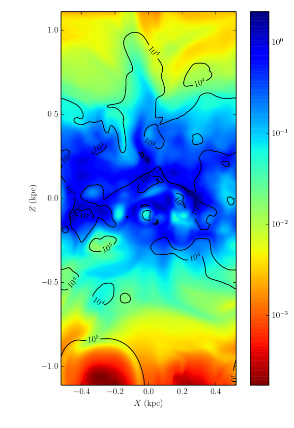
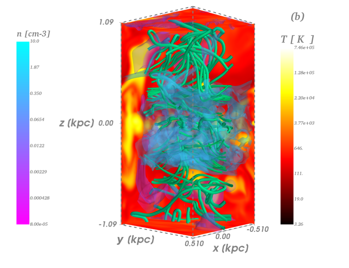
Figure 1: Left: Representative slice in the $xz$-plane of gas number density $n\,[1/\mathrm{cm}^{-3}]$ from a single snapshot overplotted with contours of temperature $T$ [K], illustrates the multi-phase ISM. Right: Snapshot of the model ISM, with temperature slices in the background and isosurfaces of the density in the foreground, with fieldlines of the magnetic field over plotted.

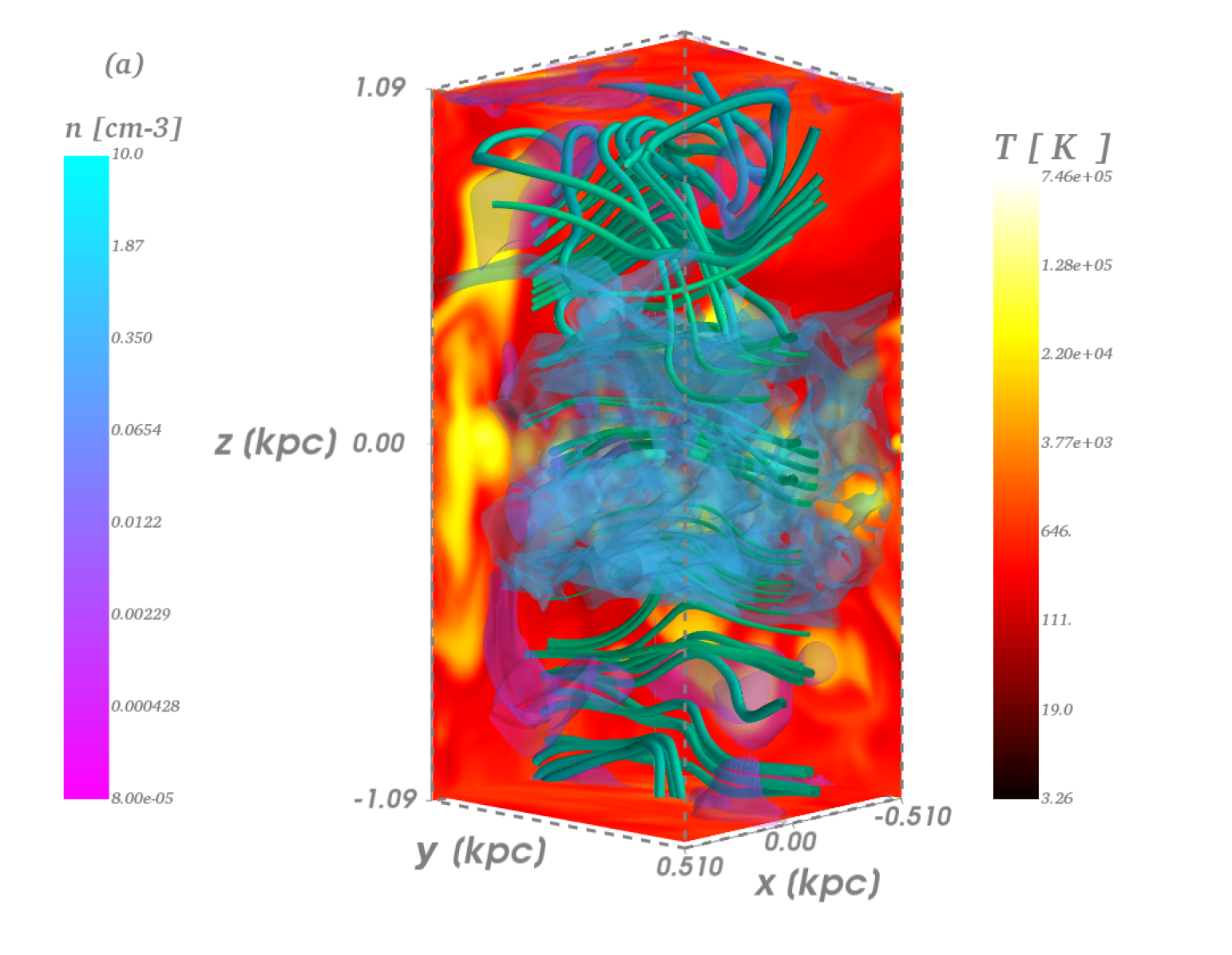
Figure 2: Snapshot of the model ISM, with temperature slices in the background and isosurfaces of the density in the foreground, as in Fig 1, but with the total magnetic $\mathbf{B}$ fieldlines replaced by $\mathbf{\bar{B}}$ fieldlines (left) and $\mathbf{b}$ fieldlines (right). For more visualisation of the MHD data, including video representation, visit http://fagent.wikidot.com/astro

2 Methods

2.1 Numerical MHD simulations

In PlanckXX, polarization statistics are compared to MHD simulations, which include cold and warm phases of the ISM. These employ adaptive mesh refinement in a computational cube 50 pc across (Hennebelle et al., 2008), from which an $18^{3}$ pc³ subset is selected for analysis. Here, we add comparisons to MHD simulations of the ISM, in which the turbulence is driven by SNe (Gent et al., 2013b; Gent, 2012, Chapters 8 & 9). In this model, the cold and warm phases are produced, as in the two-phase models, through regulation by thermally unstable radiative cooling, but with the addition of a hot phase generated by SN heating.

To capture all the relevant dynamics of the three-phase model, the simulation domain size has to be increased. The grid is $256\times 256\times 560$ and spans horizontally 1.024 kpc and vertically $\pm 1.12$ kpc about the galactic midplane. The supernova supersonic forcing naturally generates a highly shocked turbulent flow, so no artificial forcing is applied. Moreover, the interaction of rotation and anisotropic turbulence with the galactic shear flow induces a natural magnetic field through dynamo action. To model dynamo action, we solve non-ideal MHD, including viscous, thermal and magnetic diffusivities. With temperatures spanning 7–8 orders of magnitude, and high Mach numbers, it is not possible to apply the physically motivated values for diffusivity. To resolve the flows in the hot gas, while obtaining optimal small scale structure to the turbulence in the cold and warm ISM, we set the viscosity proportional to the sound speed (or $\sqrt{T}$), which may be significant for analysis in Sect. 3.1. This is not chosen to model the actual turbulent diffusivities, as little is known about their dependence on the key physical quantities in the ISM. The analytical estimates obtained in the first-order smoothing approximation framework (Steenbeck et al., 1966), however, imply that the magnitude of turbulent diffusion is orders of magnitude larger than the Spitzer molecular values. The motivation for the used viscosity scheme is to resolve much finer structures in the cool and warm ISM, than would be possible with constant diffusivity.

Note, that the resolution of $4$ pc along each side in these simulations without magnetic fields (Gent, 2012, Table 5.1) yield a maximum gas number density for the ISM of about $100\,{\rm cm}^{-3}$ and the fractional volume of the cold gas is 0.4%. The fractional volume of the warm gas is 60%, with hot gas about 28% near the SN active midplane and increasing to 41.5% elsewhere. With the magnetic field included (Evirgen et al., 2018) the model fractional volume of the warm gas increases to about 80%, the hot gas being pushed further into the halo, and the cold gas is confined to an even smaller fractional volume. A snapshot of the thermodynamic profile of the model ISM is displayed in Fig. 1 (left), wherefrom the distribution of the different gas phases is evident. Observed densities and those arising from the MHD simulations of Hennebelle et al. (2008) extend to much higher densities and increased fractional volume of cold ISM. The characteristic properties of the MHD simulation data are listed in Table 1. Temperatures, velocities and magnetic field strengths are better representatives of the observed ISM, but smallest scales of their fluctuations are limited by the grid resolution. The saturation of the magnetic field has the effect of restricting the flow and increasing the homogeneity of the ISM, so that the maximum density reduces to about 10 cm^-3, which must be taken into account when making comparisons with the Planck observations and the earlier MHD molecular cloud model. Mach number in the simulations reaches as high as 25.

			​​​​​​max​​​​​​			​​​​​​min​​​​​​
$n$	$[\mathrm{cm}^{-3}]$	5	​​​​​​– ​​​​​​	8.5	$7\cdot 10^{-6}$	​​​​​​– ​​​​​​	$2.7\cdot 10^{-4}$
$T$	[K]	$7\cdot 10^{7}$	​​​​​​– ​​​​​​	$3\cdot 10^{8}$	135	​​​​​​– ​​​​​​	311
$B$	$[\mu\mathrm{G}]$	6	​​​​​​– ​​​​​​	10		​​​​​​0 ​​​​​​
$\bar{B}$	$[\mu\mathrm{G}]$	4.6	​​​​​​– ​​​​​​	5.5		​​​​​​0 ​​​​​​
$b$	$[\mu\mathrm{G}]$	4	​​​​​​– ​​​​​​	7		​​​​​​0 ​​​​​​
$u$	$[\mathrm{km\,s}^{-1}]$	147	​​​​​​– ​​​​​​	549		​​​​​​0 ​​​​​​

Table 1: For the 12 snapshots included in the analysis, at intervals of 25 Myr, the ranges of gas number density $n$, temperature $T$, total $B$, mean $\bar{B}$, fluctuating $b$ magnetic field and speed $u$.

Both large- and small-scale dynamo instabilities are present in the system. A 3D rendition of the magnetic fieldlines embedded in this atmosphere is illustrated in Fig. 1 (right). As reported by Evirgen et al. (2017), the strength of the generated mean magnetic field at the midplane in the MHD model is in good agreement with the global observational estimates of 1.6$\mu$G by Rand & Kulkarni (1989), using pulsar RM. The random field in the model, however, is much weaker than observed, being only 20–50% of the 5$\mu$G estimate of Rand & Kulkarni (1989) or 5.5$\mu$G of Haverkorn (2015), combining RM with thermal electron density measures. These estimates are supported by the reviews of galactic magnetic fields (Beck et al., 1996; Beck, 2016). Some preliminary results applying synthetic RM measurements to the MHD model considered here are reported in Hollins et al. (2017), and further such application shall be considered in future work. The model and the characteristics of the multi-phase structure of the simulated ISM are described in detail in Gent et al. (2013a), and a summary is included in Appendix B. The coherence and fluctuations of the magnetic field are important to the polarization measurements, so it is useful to decompose the field into the mean field $\mathbf{\bar{B}}$ and fluctuations $\mathbf{b}$, where

$$\mathbf{B}=\mathbf{\bar{B}}+\mathbf{b}.$$ (1)

In this model, the entire field is subject to stirring due to the action of the many SN remnants, so the convention of separation into large-scale and turbulent components needs more careful consideration. We separate $\mathbf{B}$ by volume averaging with a Gaussian kernel (At $l=50$ pc scale, see Gent et al., 2013b). In Fig. 2 (left) $\mathbf{\bar{B}}$ fieldlines and (right) $\mathbf{b}$ fieldlines are plotted over density isosurfaces on background slices of temperature. With this treatment the ‘mean field’, which is what we shall refer to as the large-scale has strength and orientation which varies with space and time, but is coherent, i.e. similarly oriented, over scales above about 100 pc. The small-scale field is derived by subtracting the large-scale field from the total field for any given snapshot. So the large-scale field still exhibits spatial structure, which would influence polarization fractions (see Sect. 2.3). The random field is clearly incoherent and would contribute to depolarization. Some indicative values are listed in Table 1 for the ranges across the MHD snapshots of gas number density, temperature, magnetic field and speed.

The gas density $\rho$ from each snapshot is used with the radiative transfer code SOC, as described in Sect. 2.3, to model the dust temperature distribution, and the magnetic field $\mathbf{B}$ is then employed when simulating the dust polarization observations. From the velocity field we can compute directly its divergence, $\nabla\cdot\mathbf{u}$, which is also used in the analysis of the polarization to determine the influence of the shock structure of the ISM on the observations.

The simulation used for this analysis applies parameters for gas density, stellar and dark halo gravitation, galactic rotation, and SN rates and distribution matching estimates for the Solar neighbourhood. The magnetic field is amplified for a period exceeding a Gyr by dynamo action from a seed field of a few nG, which then saturates with an average field strength of a few $\mu$G. The strength of the mean field portion is consistent with observational estimates, while the random field strength is 2–5 times weaker than estimated. This has some influence on the dispersion of polarization angles in the simulated observations, discussed in Sect. 4. We use 12 snapshots from the saturated statistical steady stage of the model, each separated by 25 Myr, commencing at 1.4 Gyr. For simulated maps presented in this paper, we use the snapshot at 1.7 Gyr. The system is in a statistical steady state, so individual snapshot characteristics are representative, but strong temporal and spatial differences are also present. For some of the analysis we consider ensemble averages of the snapshots to identify the most persistent structures.

2.2 Stellar radiation field

Dust in the ISM is illuminated by the stellar radiation field. We invert the measurements of the average stellar radiation field in the solar neighbourhood from Mathis et al. (1983) into a distribution of radiation sources, to model the stellar radiation for our radiative transfer model. We then model this radiation with a horizontal density profile (see Gent et al., 2013a, excluding the dark matter component), and emissivity $j_{\nu}$ reflecting the vertical distribution of stars as

$$j_{\nu}(z)=j_{\nu,0}\exp\bigg{[}a_{1}\bigg{(}z_{\mathrm{a}}-\sqrt{z_{\mathrm{a}}^{2}+z^{2}}\,\bigg{)}\bigg{]}.$$ (2)

Here $a_{1}=4.4\cdot 10^{-14}$ $\mathrm{km}\,\mathrm{s}^{-2}$, $z_{\mathrm{a}}=200.0$ $\mathrm{pc}$ and $j_{\nu}$ is the emissivity over the spectrum of frequencies $\nu$. The normalization coefficients, $j_{\nu,0}$, are determined to return the expected total intensity $J_{\nu}$ from

$$J_{\nu}=\frac{V}{4\pi N}\sum_{i}^{i=N}\frac{j_{\nu}(z_{i},j_{\nu,0}=1)}{4\pi d}e^{-\tau_{i}}$$ (3)

where $d=\sqrt{z^{2}+r^{2}}$, $V=2\pi Z_{0}R_{0}^{2}$ and $\tau$ is the optical depth along the line of sight (LOS). The distribution is generated using Monte-Carlo method, and it is scaled to match $J_{\nu\mathrm{,Mathis}}$ from Mathis et al. (1983). Using this inversion, we obtain an approximate $z$-dependent radiation field, which produces reasonable dust temperatures with our radiative transfer simulations.

2.3 Radiative transfer calculations

To calculate the dust emission, we use the program SOC, which is a new Monte Carlo code for continuum radiative transfer against the CRT program (Juvela, 2005) and also against several other codes participating in the TRUST benchmark project on 3D continuum radiative transfer codes (Gordon et al., 2017). The density distribution of the models can be defined with regular or modified Cartesian grids or hierarchical octree grids. In this paper, all calculations employ regular Cartesian grids. In addition to the density field, the program needs a description of the dust grains (i.e. absorption and scattering properties) and of the radiation sources. The program employs a fixed frequency grid to simulate the radiation transport at discrete frequencies, one frequency at a time. The information of the absorbed energy is used to solve the grain temperatures for each cell of the model. The dust model could also include small stochastically heated grains. However, to predict dust emission at submillimetre wavelengths, the calculations are here limited to large grains that are assumed to remain at a constant temperature, in an equilibrium with the local radiation field. Once the dust temperatures have been solved, synthetic images of dust emission can be calculated towards selected directions or, as in the case of the present study, over the whole sky as seen by an observer located inside the model volume.

We assume a constant gas-to-dust ratio, where we follow the dust model BARE-GR-S of Zubko et al. (2004), which has been created to match the observations of typical Milky Way dust with the extinction factor $R_{v}=3.1$. For simplicity, we keep the properties of the dust similar throughout the whole computational domain. Dust properties may vary between different ISM phases, but the investigation of these effects is beyond the scope of this initial study.

During the simulation of the internal radiation field, the radiation transport is calculated without taking the polarization into account. However, SOC includes tools to produce synthetic polarization maps. The local grain alignment efficiency could be calculated following the predictions of the radiative torques theory (Draine & Weingartner (1996); Pelkonen et al. (2009); PlanckXX). Because our study concentrates on emission from low-density medium, this step is omitted and we essentially assume a constant dust grain alignment efficiency. The polarization reduction factor $p_{0}$ is simply set to a constant value that results in a maximum polarization fraction that is consistent with observations. Maps are calculated separately for the Stokes $I$, $Q$, and $U$ components, taking into account the local total emission, the local magnetic field direction, and the value of $p_{0}$. These data are then finally converted to maps of polarization fraction and polarization angle dispersion. A representative set of synthetic Stokes $I$, $Q$, and $U$ maps is presented in Appendix A.

To calculate the polarization within a single cell, we apply the following method. We use the Planck/HEALPix convention for the polarization angle $\psi$ (Planck Collaboration Int. XIX, 2015; Planck Collaboration Int. XXI, 2015). Within a cell we normalize the direction of the magnetic field,

$$\mathbf{\hat{B}}=\frac{\mathbf{B}}{\|B\|}$$ (4)

and calculate $\psi$ with

$$\psi=\frac{\pi}{2}+\arctan(\mathbf{\hat{B}}\cdot\hat{\phi},\mathbf{\hat{B}}\cdot\hat{\theta})$$ (5)

where the $\hat{\phi}$ and $\hat{\theta}$ are the directional vectors of the HEALPix coordinate directions. The angle between the magnetic field and the plane-of-the-sky (POS) is

$$\cos^{2}\gamma=1-(\mathbf{\hat{B}}\cdot\hat{D})^{2},$$ (6)

where $\hat{D}$ is the direction of the LOS. Based on the non-polarized emitted intensity of the cell, $I_{\mathrm{orig}}$, we get the Stokes components $I$, $Q$ and $U$ with

$$I=I_{\mathrm{orig}}\Bigg{[}1-p_{0}\Bigg{(}\cos^{2}\gamma-\frac{2}{3}\Bigg{)}\Bigg{]}$$ (7)

$$Q=I_{\mathrm{orig}}p_{0}\cos(2\psi)\cos^{2}\gamma$$ (8)

$$U=I_{\mathrm{orig}}p_{0}\sin(2\psi)\cos^{2}\gamma.$$ (9)

To match the polarization degrees observed in the PlanckXIX and PlanckXX we set $p_{0}=0.2$.

From the integrated $Q$ and $U$ we can calculate the polarization fractions $p$ and the polarization angle dispersion functions $\mathcal{S}$ over the whole sky. Simulated $p$ and $\mathcal{S}$ yield familiar measures of system properties and allow comparison to previous studies. The polarization fraction is defined as

$$p=\frac{\sqrt{Q^{2}+U^{2}}}{I}$$ (10)

and the polarization angle dispersion function (Falceta-Gonçalves et al., 2008; Hildebrand et al., 2009; Planck Collaboration Int. XIX, 2015) as

$$\mathcal{S}(\mathbf{r},\mathbf{\delta})=\sqrt{\frac{1}{N}\sum_{i=1}^{N}\big{[}\psi(\mathbf{r})-\psi(\mathbf{r}+\mathbf{\delta}_{i})\big{]}^{2}},$$ (11)

where $\psi(\mathbf{r})$ is the polarization angle in the given position in the sky $\mathbf{r}$ and $\psi(\mathbf{r}+\mathbf{\delta}_{i})$ the polarization angle at a position displaced from the centre by the vector $\mathbf{\delta}_{i}$. The sum extends over pixels whose distances from the central pixel in the location $\mathbf{r}$ are between $\delta/2$ and $3\delta/2$. As in PlanckXIX, we calculate the dispersion function with:

$$\psi(\mathbf{r})-\psi(\mathbf{r}+\mathbf{\delta}_{i})=\frac{1}{2}\arctan(Q_{i}U_{r}-Q_{r}U_{i},Q_{i}Q_{r}+U_{i}U_{r}).$$ (12)

In addition, to be comparable with the analysis presented in PlanckXIX we apply $1\degree$ Gaussian smoothing to our simulated observations, and set $\delta=30^{\prime}$ for all calculations of $\mathcal{S}$. This sets the widest distance between points in the annulus to be $1.5$ times the size of the FWHM of the Gaussian filter. The size of the annulus is small because, according to PlanckXIX  the angle dispersion function $\mathcal{S}$ gradually loses its coherence with increasing $\delta$. PlanckXIX also note that their measurements of $\mathcal{S}$ are not an artefact of either the choice of $\delta$ itself or instrumental bias. However, the small annulus will include some influence due to spatial correlations induced by the $1\degree$ beam. The choice of $\delta$ is independent of our radiative transfer model, and its primary justification is to compare our results with PlanckXIX.

We have calculated our results with several integration distances $R_{\mathrm{max}}$, namely $R_{\mathrm{max}}=0.25$, $0.5$, $1$, $2$, $4$ kpc, to explore the effect of depth. A part of the emission observed in Planck XIX is received from distances larger than what our model is capable of exploring However, with this in mind, our motivation is to inform, with an independently and physically generated ISM and magnetic field, how the impact of near and distant features might contribute to the observed images. We assume periodic boundary conditions in the horizontal direction of the computational domain. However, if the boundary is crossed in the vertical direction, the integration stops at that point, as happens in the cases $R_{\mathrm{max}}=2$ and $4$ kpc. Note, for our analysis, we mask latitudes $|b|>45\degree$ from our maps. This more closely reflects the region of the sky where the Planck observations are included in the analysis of PlanckXIX. This is an arbitrary choice, as we are not limited by the signal-to-noise issues of PlanckXIX. However, this has also other benefits. It avoids the problem of calculating $\mathcal{S}$ near the poles and some of the issues of asymmetry, caused by the limited vertical extent of the domain, that would affect the comparison of $R_{\mathrm{max}}\leq 1$ kpc and $R_{\mathrm{max}}\geq 2$ kpc. To save space, we omit from the figures related to the case with $R_{\mathrm{max}}=0.5$ kpc, but the results are similar to $R_{\mathrm{max}}=1$ kpc.

2.4 Combining data into 2D-histograms

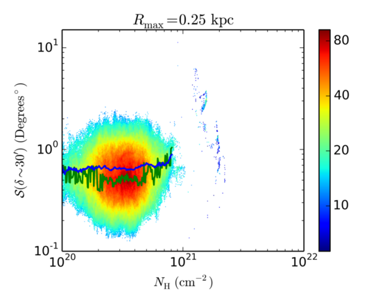
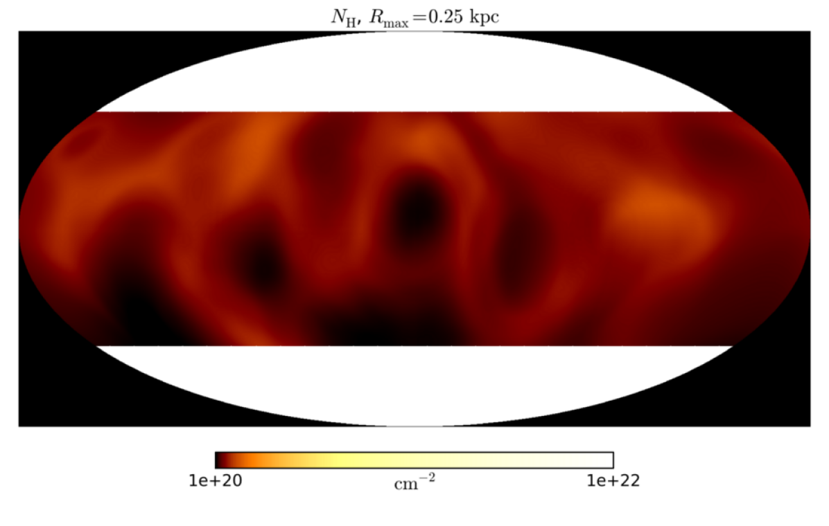
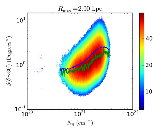
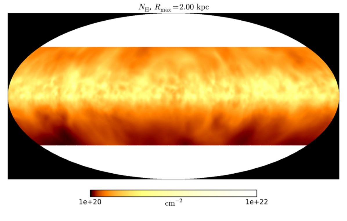
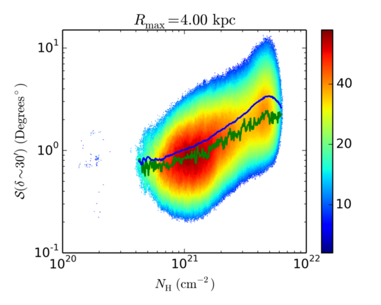
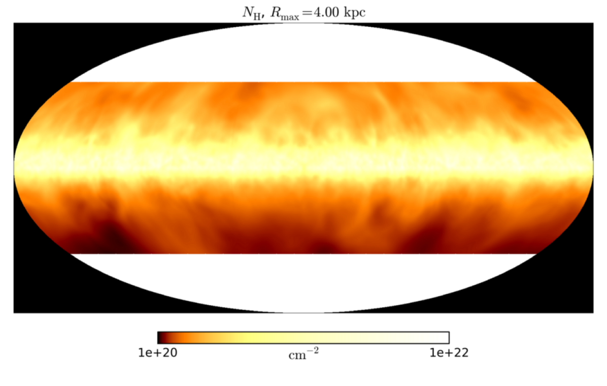
Figure 3: Left: Joint 2D-histograms of polarization angle dispersion $\mathcal{S}$ and column density $N_{\mathrm{H}}$. The green lines follow the maximum $C_{\mathrm{bin}}$ as a function of $N_{\mathrm{H}}$, and the blue lines present the weighted mean of $\mathcal{S}$. Right: Sample maps of column density. For the case $R_{\mathrm{max}}=1\,\mathrm{kpc}$, see Fig. 13.

Many of the results in this paper are represented using joint 2D-histograms. This allows us both to compare our results directly to the analysis in PlanckXIX and PlanckXX, and separate the snapshot and point-of-view (POV) specific details from the general large-scale behaviour.

For 2D-histograms, we combine radiative transfer simulations from all 12 snapshots and for 5 different POV positions in the approximate midplane, specifically from the points $(0.5,0.5,1.0)$ kpc, $(0.25,0.5,1.0)$ kpc, $(0.5,0.25,1.0)$ kpc, $(0.75,0.5,1.0)$ kpc and $(0.5,0.75,1.0)$ kpc, under the assumption that the use of periodic boundary conditions in $x$- and $y$-directions should give a reasonable representation of the ISM in the neighbourhood of the Solar System.

The data is combined as follows. From each SOC-generated map, $i$=1-60, separate 2D-histograms are constructed over a common set of $512\times 512$ bins for each comparison, specifically $C_{\mathrm{bin,i}}(N_{\mathrm{H}},p)$, $C_{\mathrm{bin,i}}(N_{\mathrm{H}},\mathcal{S})$, $C_{\mathrm{bin,i}}(p,\mathcal{S})$. Here $C_{\mathrm{bin,i}}$ represents the number of counts in a single bin calculated from a single synthetic observation. Then, assuming $C_{\mathrm{bin,i}}$ to be lognormally distributed between separate 2D-histograms, we calculate the mean and standard deviation over $i$,

$$\log C_{\mathrm{bin}}=\langle\log C_{\mathrm{bin,i}}\rangle,\quad\sigma_{\log C_{\mathrm{bin}}}=\sigma(\log C_{\mathrm{bin,i}}).$$ (13)

We include only the bins $C_{\mathrm{bin}}$ for which $C_{\mathrm{bin,i}}>0$ for all $i$. Second, to reduce additional noise, we mask out the elements where

$$\exp(\log C_{\mathrm{bin}}-\sigma_{\log C_{\mathrm{bin}}})<5,$$ (14)

yielding the composite 2D-histograms, as presented in Fig. 3 and subsequent 2D-histogram figures. Combined 2D-histograms, summing counts over many snapshots and POV, contain the patterns most consistent across the individual 2D-histograms. Despite masking low count noise, many low-frequency outliers persist.

The various simulated observations may each exhibit distinct features worthy of further analysis in the future. However, in this study we focus on the general behaviour of the system. For example, the 2D-histograms only include pixel-by-pixel numerical values. Therefore, such analysis cannot regard the filament-like shapes visible in $\mathcal{S}$-maps (See Figs. 9, 5 and 14).

3 Properties of synthetic polarization observations

Here we present our results and analysis based on the synthetic observations obtained using SOC with polarization tools on top of our MHD simulations. For our analysis, we use the maps of column densities $N_{\mathrm{H}}$, polarization fractions $p$ and polarization angle dispersions $\mathcal{S}$. As discussed in Sect. 2.1, we take (in the figures) as the reference case the 1.7 Gyr snapshot, where the observer is situated in the centre of the computational domain. We opt for projection onto a sphere as the most appropriate observational reference frame. With the domain spanning over 1 kpc in each direction, it is too large to be treated as a single observation along a Cartesian coordinate. Thus, projection onto a sphere is the most realistic observational frame, and especially so when nearby regions are concerned. The all-sky point of view affords the best comparison with Planck on the scales relevant to the MHD model. All of the maps of synthetic observations over the whole sky are presented using Mollweide projection.

3.1 Simulated column density

The maps of column density resulting from integrating over each distance, up to $R_{\mathrm{max}}=0.25,\,2$ and 4 kpc from the observer, are shown in Fig. 3, right panels. The dependence of $N_{\mathrm{H}}$ on $R_{\mathrm{max}}$ is immediately apparent. The densest regions are situated near the midplane, as would be expected from horizontal averaging of the gas density in the MHD model represented in Fig. 1. However, this is not visible on the map from $R_{\mathrm{max}}=0.25$ kpc, but clear for the higher $R_{\mathrm{max}}$. The vertical anisotropy in the latter reflects the temporal upward shift of the disk centre of mass, evident from Fig. 1. Also, density should be near isotropic in the latitudinal direction, because we do not model the galaxy’s central bulge nor spiral arms. In a single snapshot, however, local SN bubbles or superbubbles (merging multiple SN remnants) may inject significant anisotropy into the overall density profile. This is clearly seen only for the $R_{\mathrm{max}}<1$ kpc, with bubbles apparent on several locations. For the higher lengths of integration the influence of features near to the observer is almost negligible. As the combination of nearby and far-away emission will be present in both real and synthetic observations, exploring the effect of distance to the observations is called for.

Fig. 3, left panels, show joint 2D-histograms of polarization angle dispersion $\mathcal{S}$ and column density $N_{\mathrm{H}}$ for $R_{\mathrm{max}}=0.25,\,2$ and 4 kpc. At 0.25 kpc, $N_{\mathrm{H}}$ is clustered around only $1.5\cdot 10^{20}$ cm^-2 and $\mathcal{S}<1\degree$, while its corresponding $N_{\mathrm{H}}$ map, dominated by local gas structure, is without dense clouds. This is inconsistent with PlanckXIX and indicates that the integration length is too short. For higher $R_{\mathrm{max}}$, $N_{\mathrm{H}}$ is typically above $10^{21}$ cm^-2 and consistent with the observed column density featured in PlanckXIX, Fig. 24 upper panel. $\mathcal{S}$ also increases above 1, but not to the level obtained by PlanckXIX. The high $R_{\mathrm{max}}$ maps of $N_{\mathrm{H}}$ also capture the presence of these clouds, particularly evident near the midplane.

On these joint 2D-histograms are also plotted lines of maximum $C_{\mathrm{bin}}$ (green) and weighted mean (blue) polarization fractions as functions of $N_{\mathrm{H}}$. For $R_{\mathrm{max}}\gtrsim 1$ kpc the trend has a positive correlation with $N_{\mathrm{H}}$, in disagreement with PlanckXIX Fig. 24. There is no record in PlanckXX on how this relationship applies to their MHD model. Comparing our synthetic observations with PlanckXIX Fig. 24, there is a peak in the weighted mean profile for high column density dust. This corresponds to the molecular clouds, which are not resolved in the MHD model. In Fig. 3 ($R_{\mathrm{max}}>1$ kpc) the high column density range, representing the warm and cold ISM, is a good match for the PlanckXIX data. In the PlanckXIX data, however, the weighted mean remains as high or even increases at lower densities, while our simulations show a correlation ${\cal S}\propto N_{\mathrm{H}}^{0.5}$ in this range of column densities, being in obvious disagreement.

Let us try to understand this discrepancy by assuming that the small-scale scatter seen through $\cal{S}$ is a result of the underlying turbulent diffusion, taking the action of smoothing the flow. If this was the case, one would expect the higher viscosity regions smooth out structures, also those seen in $\cal{S}$, more efficiently, that is a relation ${\cal{S}}\propto\nu_{t}^{-1}$ would be expected, where $\nu_{t}$ is a turbulent diffusion coefficient related to turbulent mixing, not necessarily to any dependence assumed in viscosity scheme used in the model. As explained in Sect. 2.1, gas viscosity is set as $\nu\propto T^{0.5}$ so as to resolve flows in the hot gas of the MHD model. The ISM is modelled as an ideal gas, with all phases in approximate statistical pressure balance, so this is statistically equivalent to $\nu\propto\rho^{-0.5}$. For the radiative transfer calculations, the dust density is assumed proportional to the ISM gas density. If higher viscosity in the hot gas tends more proportionally to smooth small-scale structures in the flow, we might expect the dispersion ${\cal S}\propto N_{\mathrm{H}}^{0.5}$, which we indeed see for the low-density hot gas. This implies that the diffusion in the hot gas reflects the dependence input through the viscosity scheme, while the one for the cold and warm gas does not do so, but is somewhat steeper than expected from this simple argumentation.

We have no reliable method to determine observationally what is the true turbulent viscosity in the ISM. Some elaborate and approximate methods make this possible within numerical experiments (see, e.g., Käpylä et al., 2018). Our simple hypothesis presented above could be tested by applying the same analysis in this paper to MHD simulations with alternative prescriptions for viscosity, to exclude a relationship between the weighted mean profile and the viscosity, as appears to exist here. However, if MHD models consistently display such a dependence on viscosity $\mathcal{S}\propto\nu^{-1}$ for the weighted mean $\cal{S}$, then we might be able to infer something about the actual turbulent viscosity in the ISM from the PlanckXIX profiles. Using PlanckXIX with the weak negative correlation in between the weighted mean values of $\cal{S}$ and $N_{\rm H}$ would imply $\nu\propto T^{-\lambda}$ for the ionized ISM, with $0<\lambda\ll 1$. This is quite unlike, e.g., Spitzer molecular viscosity $\nu\propto\rho^{-1}T^{2.5}$. The scale of such simulations place that investigation beyond the scope of the present study, and of course there are many complicating factors which would permit alternative explanations of this trend.

At the lowest $R_{\mathrm{max}}$ the visible cloud structure in the $N_{H}$ map is directly tracing our MHD model. With increasing $R_{\mathrm{max}}$ smaller details appear in the maps, which are the effects of projection from more remote sources. Hence, the observed results are inevitably a combination of both the MHD model volume and its projection through a mixture of features along the LOS. By assuming periodicity in the horizontal direction, we can reach higher $R_{\mathrm{max}}$ than the physical scale of our MHD model. However, with too high $R_{\mathrm{max}}$ the periodicity creates a mirror gallery effect of repeating patterns near the $x$- and $y$-axes of the MHD model. To avoid this, it is reasonable to restrict the highest integration distance to $R_{\mathrm{max}}=2$ kpc, or for the general case, $R_{\mathrm{max}}\lesssim 2L_{x}$, where $L_{x}$ is the horizontal extent of the MHD model.

3.2 Polarization fraction across the galactic plane

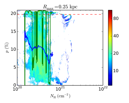
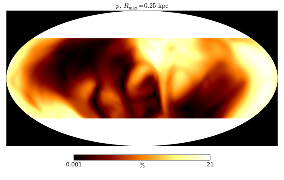
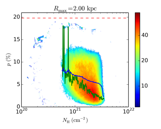
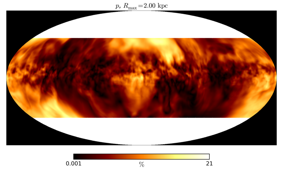
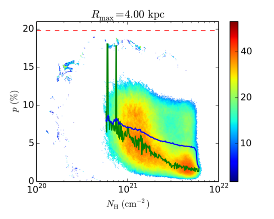
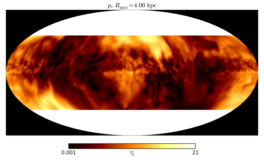
Figure 4: Left: Joint 2D-histograms of polarization fraction $p$ and column density $N_{\mathrm{H}}$. Red dashed lines show the location of $p_{\mathrm{max}}=19.8\%$ from PlanckXIX. The green lines follow the maximum $C_{\mathrm{bin}}$ as a function of $N_{\mathrm{H}}$, and the blue lines present the weighted mean of $p$. Right: Sample maps of $p$. The polarization fractions are weakened in the galactic midplane, which is seen in the 2D-histograms as a growing distribution of low $p$ at high $N_{\mathrm{H}}$. For $R_{\mathrm{max}}=1\,\mathrm{kpc}$, see Figs. 14 and 13.

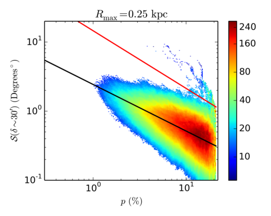
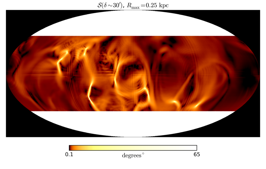
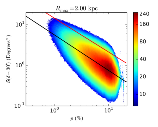
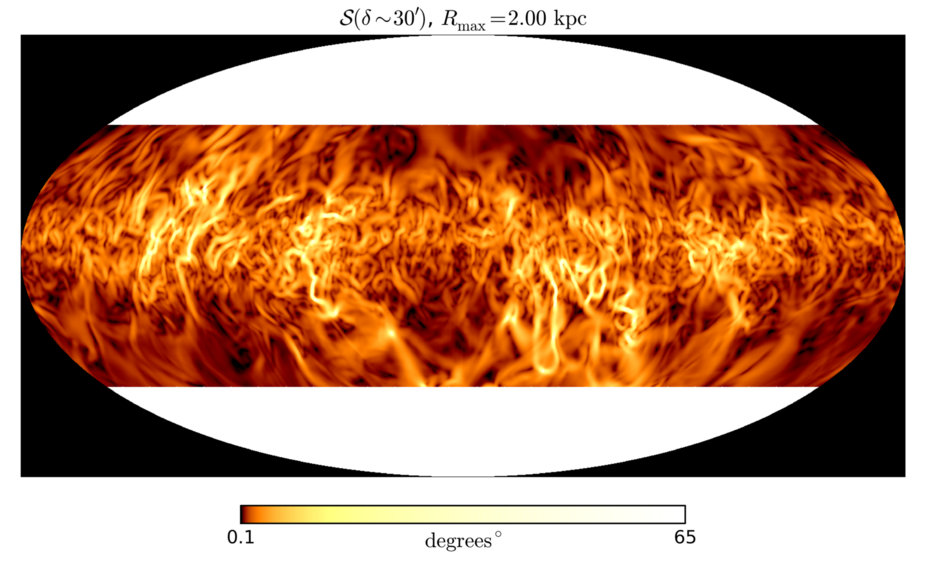
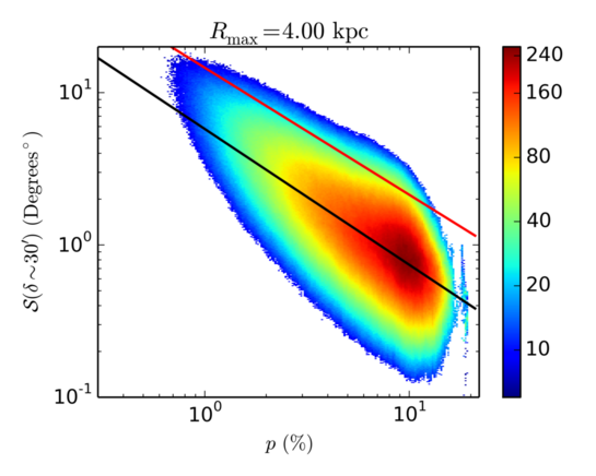
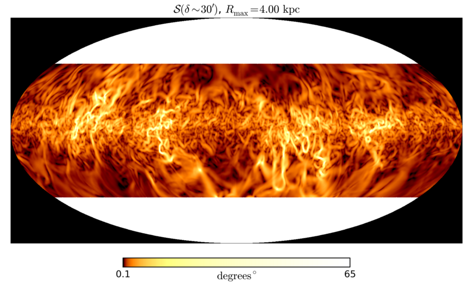
Figure 5: Left: Joint 2D-histograms of angle dispersion and polarization fraction, with the effect of increasing $R_{\mathrm{max}}$. The red line depicts the fit to the observations as presented in PlanckXIX, $\log_{10}\mathcal{S}=\alpha\log_{10}p+\beta$. The black lines are the best fits to our simulated data, to which $\alpha$ and $\beta$ are given in the Table 2. Right: Sample maps of polarization angle dispersion $\mathcal{S}$ with corresponding $R_{\mathrm{max}}$.

For each $R_{\mathrm{max}}$ we construct joint 2D-histograms of polarization fraction $p$ and $N_{\mathrm{H}}$, presented in Fig. 4, left panels, and the maps of $p$, right panels. With $R_{\mathrm{max}}=0.25$ kpc there is a broad range for $p$ values. The distribution is independent of the $N_{\mathrm{H}}$ values, which in this case are much lower than in the PlanckXIX observations. The mapping of $p$ can be seen to correlate over large smooth regions. There is negligible depolarization, with the highest $C_{\mathrm{bin}}$ appearing on the scale of $p_{0}=20\%$.

With $R_{\mathrm{max}}=2$ kpc depolarization is stronger, particularly near the midplane, the map of $p$ being an excellent analogue for PlanckXIX, Fig. 6. Its 2D-histogram is also a better match with PlanckXIX, Fig. 19, although $N_{\mathrm{H}}>10^{22}$ cm^-2 are absent and there are few values with $p>15\%$. The high column density may relate to features not modelled with the MHD, such as the central bulge, spiral arms, and molecular cloud properties requiring higher resolution to be resolved. Some of the absence of higher $p$ is due to the masking of bins which lack signal across all synthetic maps cobined to the 2D-histogram in question. In addition, the fraction of the PlanckXIX data, which has $p>15\%$, is concentrated into the molecular cloud complexes, where high polarization fractions can be found, which are among the features not resolved in our MHD models.

The increased frequency of $p>5\%$ with $R_{\mathrm{max}}=4$ kpc is more like the PlanckXIX results, but the high number of points where $p<5\%$ and $N_{\mathrm{H}}\simeq 5\cdot 10^{21}$ cm^-2 is not consistent with PlanckXIX, and an indication that oversampling the same periodic domain near the midplane is distorting the distribution. To improve the range of column densities in a physically consistent manner, one should increase the horizontal extent of the MHD models. Also, increasing the MHD model resolution would improve both the proportion of high column densities and high polarization fractions, but this would be computationally demanding in the context of SN-driven MHD turbulence that is capable of producing self-consistent small- and large-scale dynamos.

Regardless of these current limitations, it is interesting to consider how the distances influence polarization and depolarization. In the framework of the radiative transfer calculations, the mechanism is easy to understand. Along the LOS, individual cells in the grid produce positive and negative contributions in $Q$ and $U$, depending on the local magnetic field direction. For an incoherent magnetic field, the sign of $Q$ and $U$ fluctuates, with similar magnitude, such that over very long distances in an optically thin medium their averages approach zero. This is comparable to the analysis of Houde et al. (2009), where they note that multiple independent turbulent cells along the line of sight will make the apparent fluctuation to approach zero. However, the mean field also varies in direction when exploring kiloparsec scales which will also contribute to the perceived effect. In the presence of a directionally coherent magnetic field, its direction will dominate the $Q$ and $U$ over long distances. However, the magnetic fields are highly turbulent throughout the MHD domain, so we expect depolarization to increase with $R_{\mathrm{max}}$.

Near the midplane the depolarization effect is strongly proportional to integration length with $R_{\mathrm{max}}\geq 2$ kpc (Fig. 4, lower right panels), corresponding high $N_{\mathrm{H}}$. This is also consistent with the above explanation. Near the midplane with large $R_{\mathrm{max}}$ it is possible to integrate polarization over a longer distance, unlimited by the upper or lower boundaries of the computational domain. Therefore, there is more influence on $p$ from the depolarizing effect of the fluctuations, most evident near the midplane. The role of magnetic field fluctuations inducing a broad spread of $p$ has also been suggested by PlanckXIX and PlanckXX  and our results support this idea.

Due to the averaging and masking method presented in Sect. 2.4 some of the outlying values persist as halos in the 2D-histograms of Fig. 4 (also Fig. 13), but with higher sampling rates, the masked points between the bulk data and halo could be restored. Also, the gradual loss of alignment of the dust grains within radiation shielded dense clouds can decrease polarization, which is also considered by PlanckXIX to be an effect influencing their observed depolarization with $N_{\mathrm{H}}\geq 10^{22}$ cm^-2. We set the strength of alignment proportional to $p_{0}$ in Eqs. 7-9, neglecting any effects of such shielding.

As our methods resemble those of PlanckXX, some dicussion is called for, although we cannot make a direct comparison of their MHD model with our results. They consider scales well below our 4 pc grid resolution. What is relevant, is that the structure of the flow and the magnetic field in our MHD model is naturally driven by the forces on the scales of SN remnants cascading to the lowest turbulent eddies we can resolve. It is reasonable to expect that the turbulent structure would extend to lower scales, until new physical processes become active.

PlanckXX compare their MHD results with observations of the Chamaeleon-Musca and Ophiuchus fields. For their MHD simulation, they view the domain with respect to the mean field as POS, LOS and 50/50, confirming that a high polarization fraction is indicative of a strong POS component to the field. This is evidence that the magnetic field has a strong POS component in Chamaeleon-Musca, while in Ophiuchus the field is more aligned along the LOS, an interpretation consistent with Planck Collaboration Int. XXXV (2016), their Fig. 3, which shows a more consistently ordered POS field for Chamaeleon-Musca compared to that of Ophiuchus.

For all three cases examined in PlanckXX, the values in the polarisation fraction distribution are low compared to either Chamaeleon-Musca or Ophiuchus. It may be that the random component, and hence depolarization, in the MHD models was too strong. Alternatively, the forcing mechanism they use induced a Gaussian distribution to the magnetic field, while our analysis, with SN-driven turbulence, indicates it to have more exponential distribution, which could influence the efficiency of the depolarization (see Sect. 3.3). With respect to the mean field component Gent (2012, Ch. 9 Fig. 9.12), find that the magnetic fields in the cold filamentary regions formed by SN driven turbulence are more regular than the ISM as a whole and that they are strongly aligned with the ambient warm ISM, in which they are embedded. This is in contrast to the observations of Planck Collaboration Int. XXXII (2016); Planck Collaboration Int. XXXIII (2016), who found the orientation of the filamentary structure of the most dense molecular clouds to be perpendicular to the mean magnetic field. Here, gravitational collapse and runaway thermal instabilities leading to the formation of such high density structures may be critical, which are absent on the scales considered in our MHD model.

3.3 Polarization angle dispersion

Looking at the maps of polarization angle dispersion $\mathcal{S}$ presented in Fig. 5 (right panels), we observe filamentary structures ($\mathcal{S}$-filaments) similar in appearance to PlanckXIX Fig. 12. However, for $R_{\mathrm{max}}=0.25$ kpc these are very large scale structures, which span the full range of examined galactic latitudes in some locations and are much thicker than the PlanckXIX observations. With increasing $R_{\mathrm{max}}$ the $\mathcal{S}$-filament structure resembles quite well PlanckXIX Fig. 12, becoming tangled and fragmented, increasing in number and having more wiggles. PlanckXX report filament-like maps of $\mathcal{S}$ from their synthetic observations. However, due to the differences in scale, resolution and forcing mechanism behind the MHD model used in PlanckXX and this study, an effective qualitative comparison is not reasonable.

$R_{\mathrm{max}}$ (kpc)	$\alpha$	$\beta$	$\langle\mathcal{S}/\mathcal{S}_{\mathrm{Planck}}\rangle$	Notes
–	$\mathbf{-0.834}$	$\mathbf{-0.504}$	$100\%$	Planck
0.25	$-0.673$	$-0.961$	$24\%$
0.5	$-0.742$	$-0.898$	$32\%$
1.0	$-0.789$	$-0.920$	$34\%$
1.0	$-0.934$	$-1.020$	$39\%$	$2\cdot\mathbf{b}$
2.0	$-0.876$	$-0.999$	$35\%$
4.0	$-0.892$	$-1.021$	$35\%$

Table 2: Fits to $\log_{10}\mathcal{S}=\alpha\log_{10}p+\beta$ for each joint 2D-histogram of $\mathcal{S}$ and $p$. The observed values are from the best fit of PlanckXIX.

In Fig. 5 (left panels) the joint 2D-histograms of $\mathcal{S}$ and $p$ show some agreement with Fig. 23 of PlanckXIX. Angular dispersion is inversely proportional to polarization fraction, and may be approximated by

$$\log_{10}\mathcal{S}=\alpha\log_{10}p+\beta.$$ (15)

The 2D-histograms show our best fits (black lines) for Eq. (15) and the fit from PlanckXIX (red lines). The parameters are summarised in Table 2. For $R_{\mathrm{max}}$ at 1 kpc and above, the slope $\alpha$ is near to the PlanckXIX fit, but by having smaller intercept $\beta$ our 2D-histograms are shifted to lower $\mathcal{S}$. There may be a case for inferring that the optimal integration length is about $R_{\mathrm{max}}=1.5$ kpc, if we are looking to match $\alpha$ for the PlanckXIX data. Repeating the analysis for an MHD domain with increased horizontal extent and/or increased resolution might indicate whether this is a robust physical relationship between the simulated and observed measurements. The ratio $\mathcal{S}/\mathcal{S}_{\mathrm{Planck}}=p^{\alpha-\alpha_{\mathrm{Planck}}}10^{\beta-\beta_{\mathrm{Planck}}}$ is averaged and listed in Table 2 for each $R_{\mathrm{max}}$.

The dispersion values in our simulations increase towards PlanckXIX as $R_{\mathrm{max}}$ increases, but plateau at a ratio of $35\%$ for $R_{\mathrm{max}}\gtrsim 1$ kpc. The increase to 39%, when artificially strengthening the amplitudes of the small-scale fluctuations of the magnetic field, supports the view that the low simulated value for $\beta$ is in part due to insufficient small-scale field. The low values of $\mathcal{S}$ in our MHD model may be attributed to truncated resolution at the grid scale of 4 pc.

To understand the distribution of velocity and magnetic fields in our MHD model data, we present probability density distribution functions (PDFs) of the both variables in Figs. 6 and 7. The PDFs are calculated over all MHD model cells from all snapshots where each cell, being of same volume, has an equal weight. In Fig. 6, upper panel the PDF is exponential for $B_{x}$ ($B_{y}$) and $B_{z}$, while $B_{y}$ ($B_{x}$) is skewed by the global shear. Fig. 6, lower panel, shows the PDFs for the velocity components, where within the velocity range $\pm 400$ km s^-1, the PDFs reflect ISM physics as resolved by the model. We evolve SN remnants only from the latter stages of the Sedov-Taylor phase, however, so this is exhibited in the truncated PDF for $|u|\gtrsim 400$ km s^-1.

The spiked PDF displayed in Fig. 6 for the magnetic and velocity field components arise from the physics of repetitive shock-driven turbulence, independent of the model and resolution. Few authors have discussed this property, but a similar distribution for the velocity profile is illustrated in Gressel (2010, Fig. 3.13). In their Fig. 9 Mac Low et al. (2005), using approximately 1.5 pc resolution, show similar PDF profiles for the divergence of the velocity field, also supporting this physical interpretation of the turbulent structure of the ISM.

The multiphase medium plays a role in this distribution. In Fig. 7 we divide PDFs into three components, corresponding with cold, warm and hot medium ($T<100$ K, $100\leq T<10^{5}$ K and $T>10^{5}$ K respectively). The Fig. 6 velocity profile mainly exhibits the warm phase PDF depicted in Fig. 7, apart from at high velocities where the hot phase is more visible. The PDF is approximately Gaussian for the cold phase. Based on this component separation, the sharp PDF profile of magnetic field in the hot phase, and less so for the warm, is likely connected with the large-scale compressive forcing in the warm and hot phases, and subsequent turbulent cascade. The cold phase contains a magnetic field with a distribution that is between an exponential and a Gaussian, resembling that of PlanckXX, Fig. 11, apart from having a weaker magnetic field strength. It is possible that the higher densities in the cold phase may act as a sponge for these compressions and rarefactions, but we cannot assume that the effects of the turbulent cascade driven by SN are absent even at the scale of molecular clouds.

Therefore, some caution should be attached to the velocity PDF for the cold phase for at least two reasons. In their Fig. 15 (c) Gent et al. (2013a) show that the hot phase flows are mainly subsonic, the warm transonic and the cold supersonic. However, the cold clusters are typically entrained within the bulk flows of their ambient warm gas. If the bulk velocity of the ambient warm gas were subtracted, then the Mach number of the cold phase would likely reduce, and the residual flow might retain more of the PDF structure of the hot and warm phases. Also, in this model the scale of the cold structures tend to be only a few grid spaces across, i.e., they are near the limit of the model resolution, so much of the substructure of the magnetic and velocity fields in this phase are truncated. So although the MHD model here is truncated at 4 pc, it is our contention that the physics that drive the structure of the magnetic field in the hot and warm phases are still relevant to the flow driving the dynamics at smaller scales. This would require comparison with higher resolution multi-phase turbulence simulations. Only from new physical processes, such as self-gravity, would we expect to introduce changes to the structure of the turbulence.

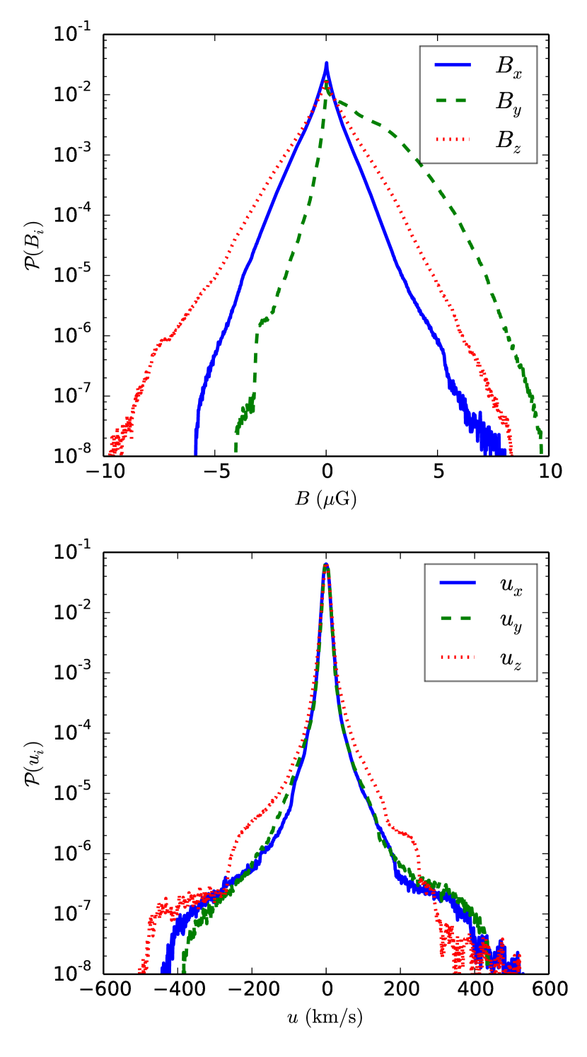
Figure 6: Probability density function combined from all 11 snapshots for the components of $\mathbf{B}$ and $\mathbf{u}$.

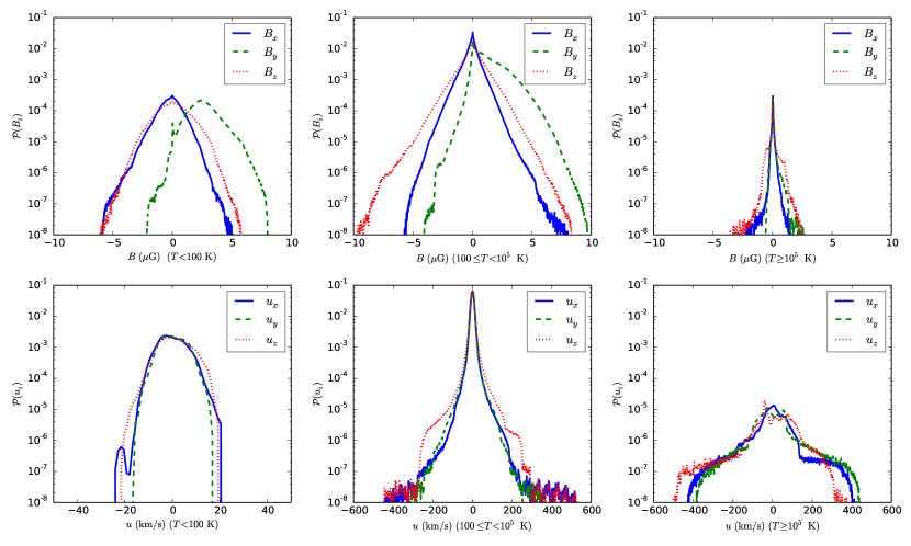
Figure 7: Probability density function combined from all 11 snapshots for the components of $\mathbf{B}$ and $\mathbf{u}$ with cold, warm and hot components separated.

4 Shock and magnetic structure interpretation

We now consider how $\mathcal{S}$-filament structures seen in the polarization angle dispersion measurements are related to physical properties of the ISM. These are difficult to measure directly through observations, but can be measured easily in the MHD models. In the analysis that follows, we mostly refer to integration along the LOS with $R_{\mathrm{max}}=1$ kpc. This range, within the properties and horizontal extent of the MHD model, is sufficient to adequately capture the key features present in the PlanckXIX observations. For more demanding analysis it would be recommended to integrate $R_{\mathrm{max}}\simeq 2L_{x}$.

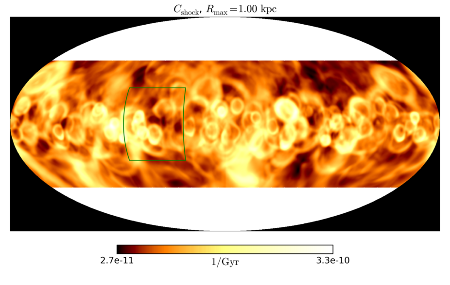
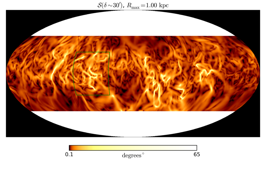
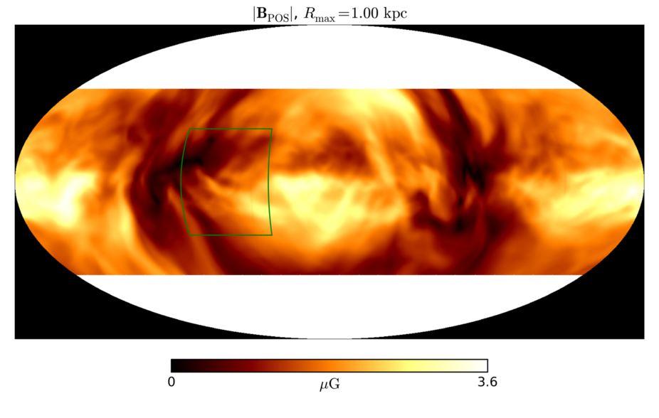
Figure 8: Top: The distribution of the average values of $C_{\rm shock}$ in the LOS. Middle: Map of polarization angle dispersion $\mathcal{S}$. Bottom: Projected average magnetic field strength in POS. The green rectangles refer to the area featured in Fig. 9. $R_{\mathrm{max}}=1$ kpc.

4.1 $\mathcal{S}$-filaments compared with shocks

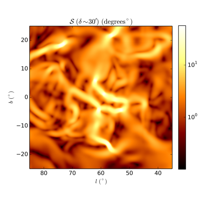
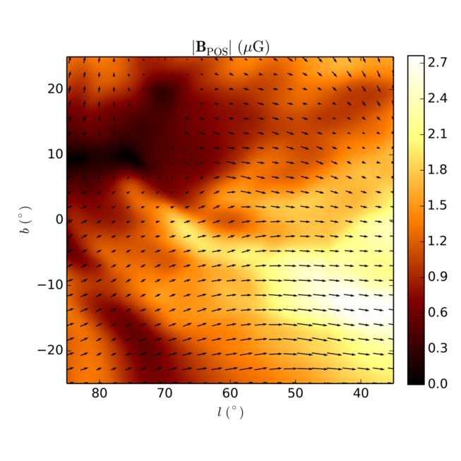
Figure 9: A local comparison of $p$, $\mathcal{S}$, $|\mathbf{B}_{\mathrm{POS}}|$, and shocks within the area marked in the Figs. 14 and 8.

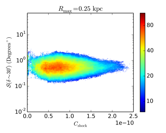
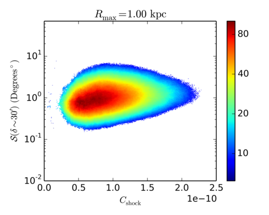
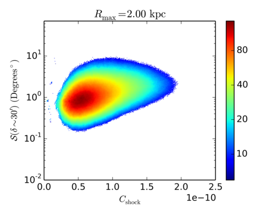
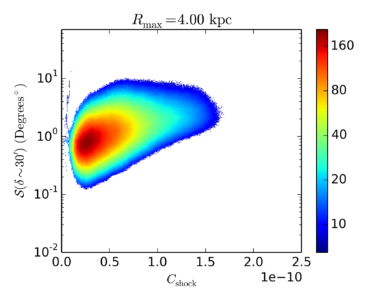
Figure 10: Joint 2D-histograms of polarization angle dispersion $\mathcal{S}$ and average LOS shock compression $C_{\rm shock}$.

Changes in the direction of polarization angle $\psi$ and therefore $\mathcal{S}$ are related to changes in the magnetic field, and these are driven and generated by SN-driven turbulence. Generally, $\mathcal{S}$ follows a lognormal distribution (see PlanckXIX  Fig. 14). The lognormal nature of the $\mathcal{S}$ distribution in the observed and simulated ISM appears consistent with the effect shocked turbulence has on the statistics of the gas density (as noted in Vazquez-Semadeni, 1994; Elmegreen & Scalo, 2004; Gent et al., 2013a), which encourages us to look into the connection between $\mathcal{S}$ distribution and shocks present in our simulation data.

To investigate the effect that the shocks have, we first compute a proxy of their magnitude, $C_{\rm shock,local}=|[\nabla\cdot\mathbf{u}]_{-}|$, where only the negative divergence contributes. This corresponds to regions where the flow is convergent, where therefore the shocks created by SNe are compressing the surrounding ISM. The values of $C_{\rm shock,local}$ are calculated within the numerical grid of the MHD model. All $C_{\rm shock}$ maps show $C_{\rm shock,local}$ averaged over the LOS up to the defined $R_{\mathrm{max}}$, or

$$C_{\rm shock}=\langle C_{\rm shock,local}\rangle_{\mathrm{LOS}}\Big{|}_{0}^{R_{\mathrm{max}}}.$$ (16)

In Fig. 8, maps are displayed for average $C_{\rm shock}$, $\mathcal{S}$, and the POS magnetic field, $|\mathbf{B}_{\mathrm{POS}}|$, averaged over the LOS up to $R_{\mathrm{max}}=1$ kpc. A zoom-in area is marked on each map, for which the local maps are displayed in Fig. 9. The joint 2D-histograms of $\mathcal{S}$ and $C_{\rm shock}$ are presented in the Fig. 10.

Apart from the energy input to the turbulence being stronger in the midplane due to the general distribution of SNe, there is no visible correlation between the SN shocks and the average POS magnetic field nor polarization angle dispersion. The 2d-histograms presented in the Fig. 10 do not show any clear dependence between $\mathcal{S}$ and $C_{\rm shock}$, apart from the effect of midplane-weighted SN-distribution being more pronounced. However, there is a large-scale pattern in the magnetic field, which is discussed in the Sect. 4.2.

Examining the zoomed-in area displayed in Fig. 9, the filamentary structures in $\mathcal{S}$ (top right panel) overlap very sharply with the areas of low polarization fraction (top left panel). There is likely a connected phenomenon, which links these effects. Directly relating this to specific physical features in the model is a challenge, because locally the alignment of polarization is a combination of effects layered on the top of each other. One approach to understanding this is to perform a series of calculations over a range of discrete integration lengths $R_{\mathrm{max}}$ and to analyse in detail how the maps change as certain features of the model are included or excluded. It is also possible to explore the relationship between magnetic fields and dispersion over large scales.

We stress that in advocating such an approach, we do not aim to explain directly particular observational features from Planck, but to inform how the inclusion or absence of physical phenomena along the LOS, which we can identify precisely in the MHD models, might be expected to contribute to the simulated observations. Such results can also be used to deepen the physical interpretation of the Planck findings.

When comparing the shock profile in Fig. 9 (bottom right panel) with the polarization angle dispersion (top right panel) the strongest filamentary structures correspond to locations where the shocks are negligible. In the upper half of Fig. 9 (bottom left panel) the strength of the POS magnetic field seems to correlate quite well with the polarization fraction (top right panel), however in the lower right quadrant of the map a strong field is anti-correlated to $p$, so the relationship is not at all straightforward. In principle, all of these relationships should be explored further by varying $R_{\mathrm{max}}$ as described above, but it appears likely that we can exclude the $\mathcal{S}$-filaments being indicative of the shock structure of the ISM.

4.2 Dispersion and the large-scale magnetic field

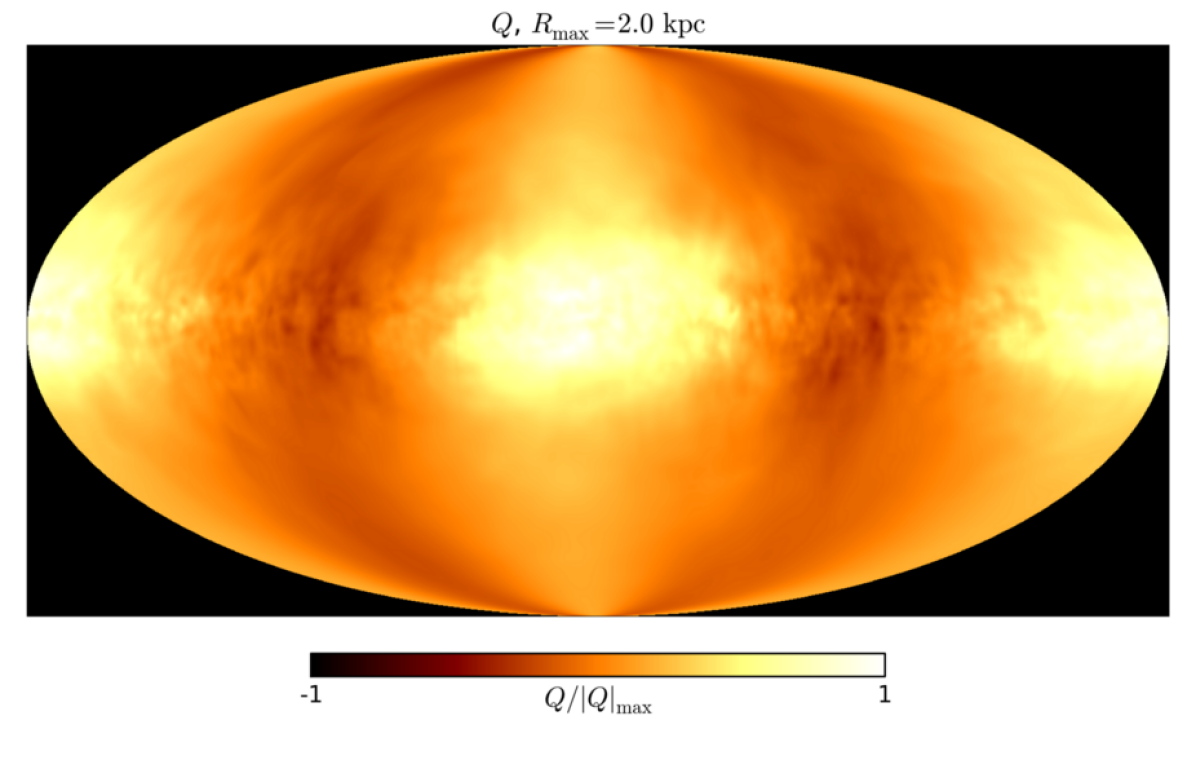
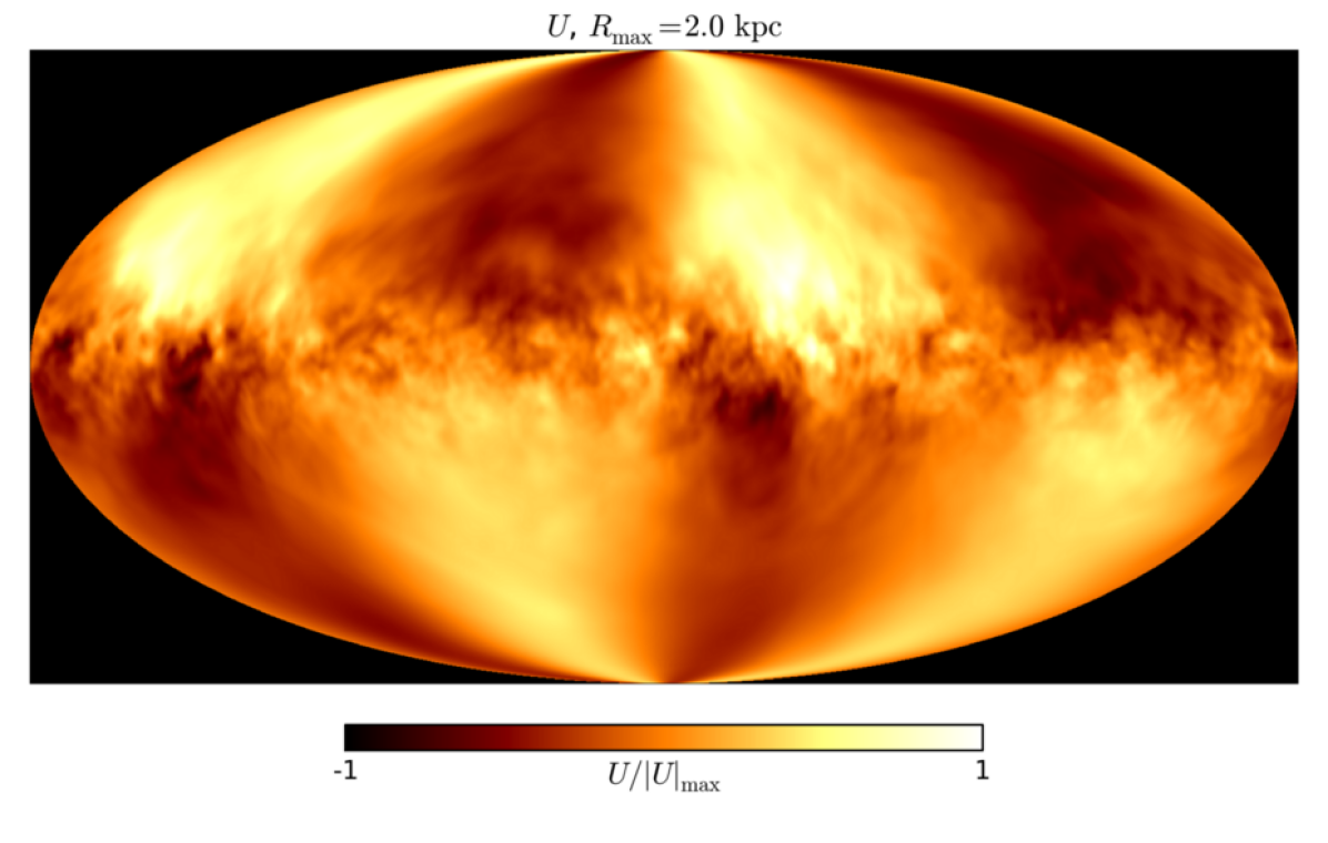
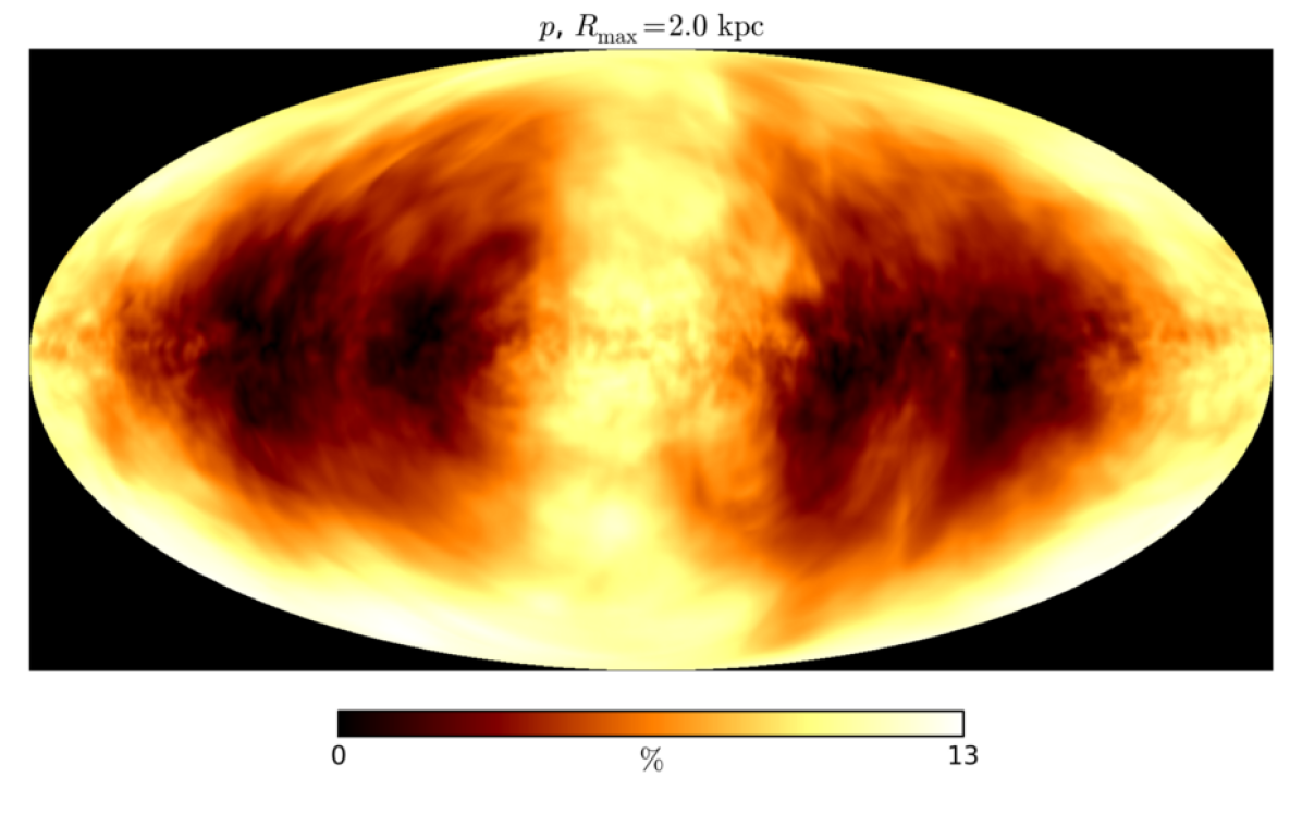
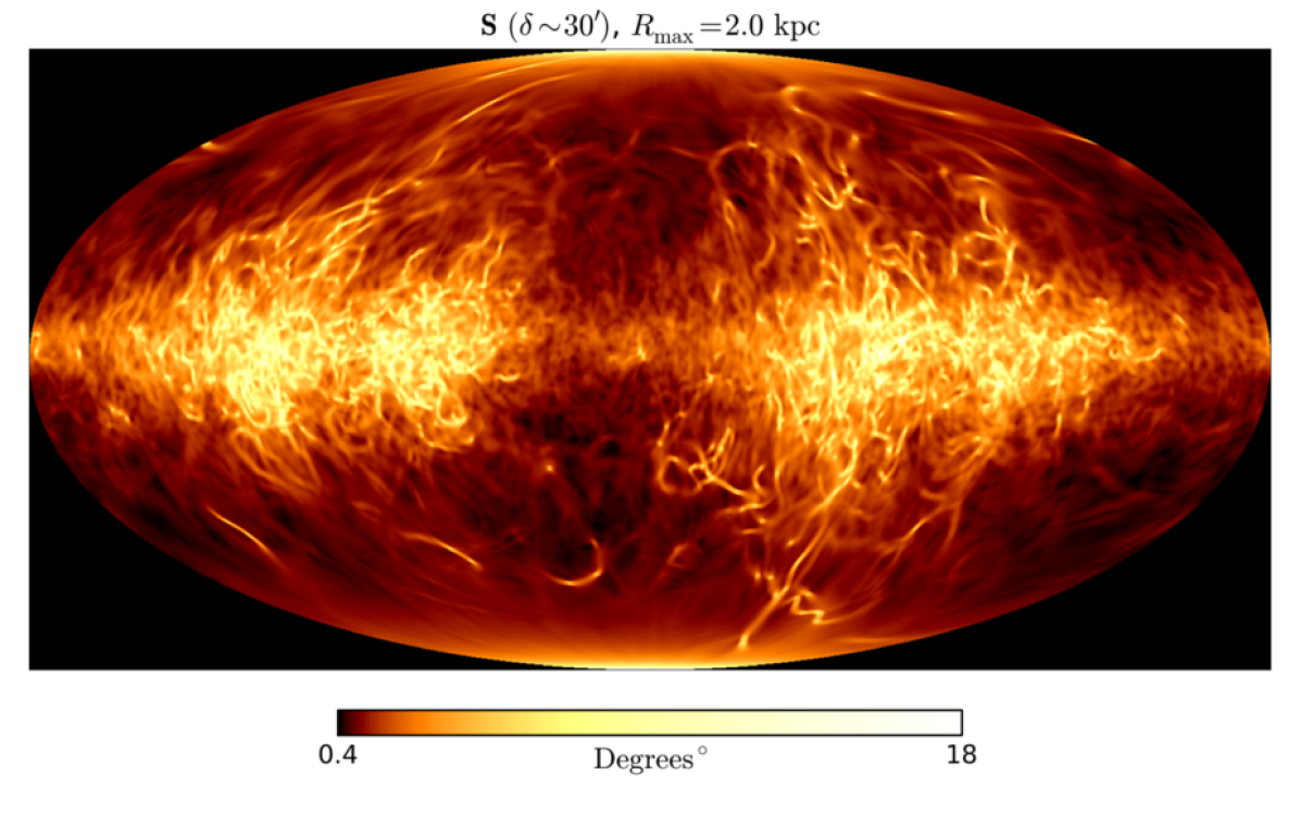
Figure 11: Averaged maps of $Q$, $U$, $p$, $\mathcal{S}$ over the all 12 snapshots.

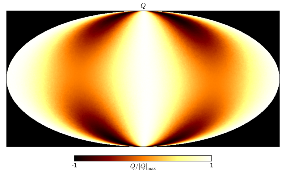
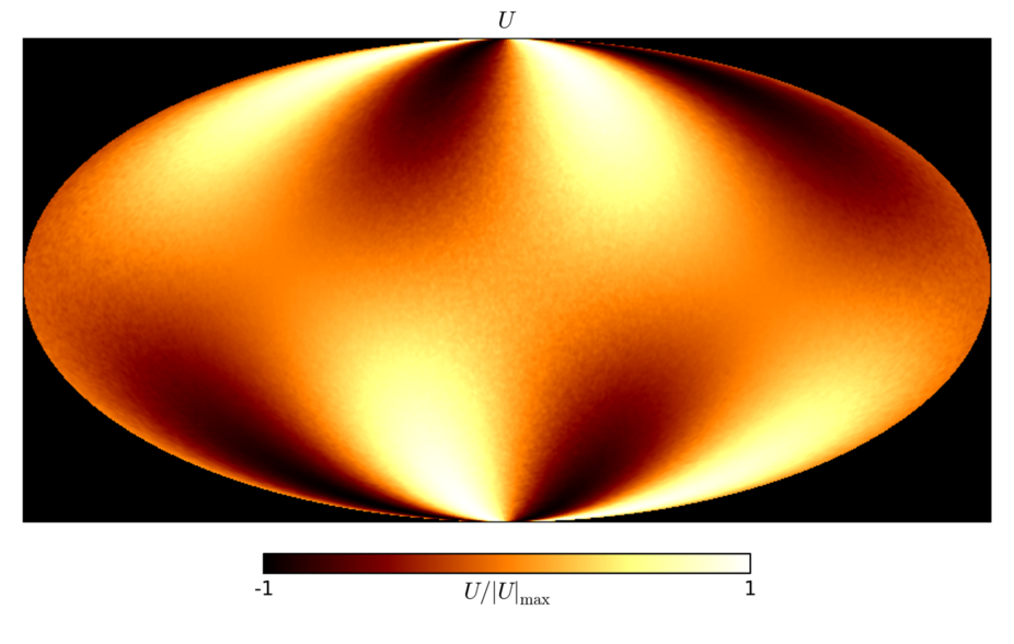
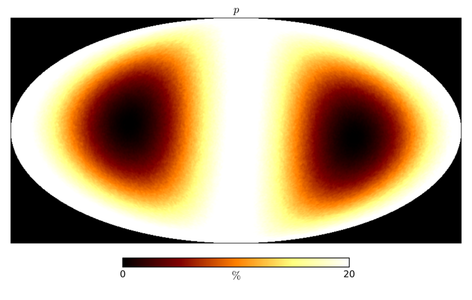
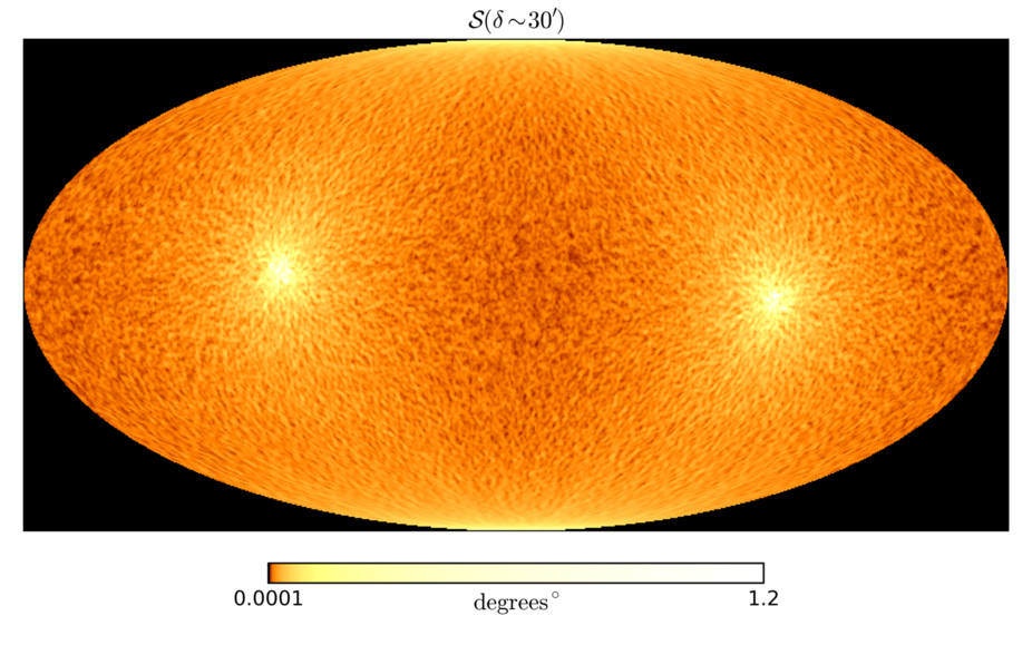
Figure 12: Distribution of polarization assuming a simple analytical model of the magnetic field as described by the Eq. 17.

Already Heiles (1996), for example, have used starlight polarization measurement to estimate the direction and curvature of the galactic magnetic field. Their results showed signs of spiral curvature, although the fluctuating component of the field is also significant. More recent studies (Planck Collaboration Int. XLII, 2016; Planck Collaboration Int. XLIV, 2016) have used the new Planck results to estimate the structural properties of the Galactic magnetic field by fitting magnetic field models to observations.

In our synthetic observations, the distribution of polarization angle dispersion exhibits a significant dependence on galactic latitude and longitude. This becomes more apparent when taking averages from all simulated observations with the same observer location, but for different snapshots, as is presented in Fig. 11 (lower right panel). The measurements of $Q$ reverse twice in one full rotation in latitude (upper left panel), while $U$ switches sign across the galactic plane and also exhibits the same latitudinal sign reversals as $Q$ (upper right panel). The polarization fractions are minimised where the brightest filamentary structures are most pronounced. The general nature of this pattern may be expected. As outlined in Sect. 2.1, the magnetic mean field is strongly aligned in the direction of the differential rotation of the model.

The dependence of polarization properties on the orientation of the mean magnetic field is a known relation. Already, in the context of turbulent molecular clouds, Ostriker et al. (2001), Soler et al. (2013) and PlanckXX have shown that distribution of fluctuations in polarization is connected with the direction of the magnetic mean fields of molecular clouds. Such analysis has also been utilized with Planck observation in relation to the molecular clouds (Planck Collaboration Int. XXXII, 2016; Soler et al., 2016). This urges us to look into this phenomenon with our modelling results. However, as we look into large-scale patterns, Planck Collaboration Int. XLII (2016); Planck Collaboration Int. XLIV (2016) provide the most fruitful points of comparison.

The upper panels of Fig. 11 are remarkably consistent with Planck Collaboration Int. XLII (2016, Fig. 13), who examine a set of galactic magnetic field models without dynamo nor SN-driven turbulence to generate a realistic field, but including the galactic centre and spiral arms, which they fit to observational data. Their synthetic maps do not have the small-scale features associated with the turbulence, but on larger scales our maps have very similar structure, the only characteristic difference being longitudinal variation caused by the included spiral arms. So, apparently, local structures in the ISM may be predominant in the observed data, although further investigation along the lines of Planck Collaboration Int. XLII (2016) and inclusion of spiral arms in a model of MHD turbulence would need to be pursued.

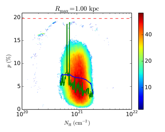
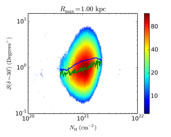
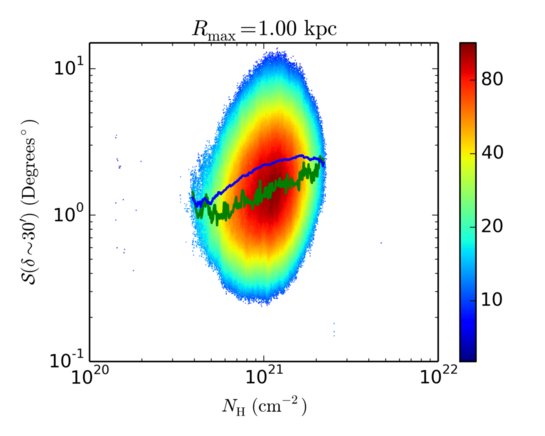
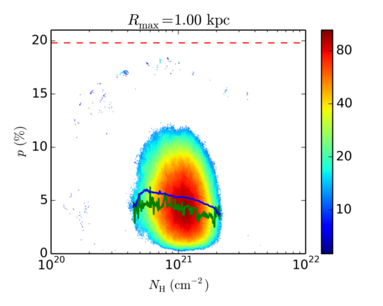
Figure 13: Joint 2D-histograms of (Top) polarization fraction and column density, (Middle) polarization angle dispersion and column density, and (Bottom) polarization angle dispersion and fraction. Red line depicts the fit to the observations as presented in Planck Collaboration Int. XIX (2015), $\log_{10}\mathcal{S}=\alpha\log_{10}p+\beta$. Black lines are the best fits to our simulated data, to which $\alpha$ and $\beta$ are given in the Table 2. Green lines follow the maximum counts in the 2D-histograms as a function of $N_{\mathrm{H}}$, and blue lines present a weighted mean of the polarization fractions. Left: Normal case. Right: Doubled perturbations case. In all cases $R_{\mathrm{max}}=1\,\mathrm{kpc}$.

The large-scale variation follows from the presence of the mean field in our MHD model. We can illustrate it with a simple analytical example starting from the first principles. Let us assume a simple uniform $y$-directional mean field with random fluctuations at the smallest scales of the grid

$$\mathbf{B}=B_{0}\hat{\bf y}+\Delta\mathbf{b}$$ (17)

where $|B_{0}\hat{\bf y}|\gg|\Delta\mathbf{b}|$. This configuration generates a large-scale structure of the polarization (see Fig. 12, and also Planck Collaboration Int. XLIV, 2016, their Fig. 4, top panels). In addition to this, the direction of the magnetic field affects the sensitivity of the observed polarization to the small magnetic fluctuations. If we apply Eq. 17 to Eqs. 4, 5 and 6 we notice that near the HEALPix coordinates $\phi\approx\pm\pi/2$ and $\theta\approx\pi/2$ the influence of the magnetic field approaches the values $\psi\approx\pi/2+\Delta\psi$ and $\gamma\approx\pi/2+\Delta\gamma$, where we have divided the contribution from the mean and the fluctuating field. Therefore, when calculating the polarization components, with Eqs. 8 and 9, we get,

$$Q\approx-Ip_{0}\cos\Delta\psi\sin^{2}\Delta\gamma$$ (18)

$$U\approx-Ip_{0}\sin\Delta\psi\sin^{2}\Delta\gamma.$$ (19)

This signifies that, when the LOS approaches the direction of the consistent mean magnetic field, the POS field is highly sensitive to small, local fluctuations caused by turbulence. This, in turn, will show up as variations in polarization angle and therefore relatively high $\mathcal{S}$. To summarize, when the strong mean field is perpendicular to the LOS, its direction dominates the polarization angles, but when the field is parallel to the LOS, the observed polarization angles are more sensitive to the small fluctuations in the field. However, the polarization fraction $p$ is weak in the mean field aligned with the LOS, as the small fluctuations themselves produce less strong $Q$ and $U$. Thus, we have a similar interpretation to PlanckXX. In their study, $\mathcal{S}$ is strongest when the POV faces towards the mean field direction, along with a weaker polarization fraction. In contrast, they observe a higher polarization fraction and a coherent polarization angle when the direction of the mean field follows the POS.

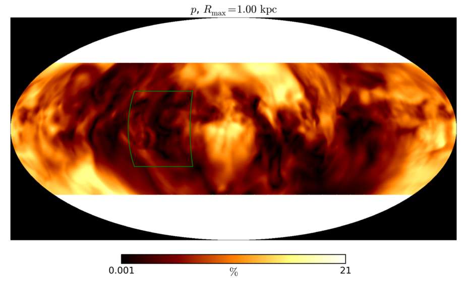
Figure 14: Top: Sample maps of polarization fraction $p$. Bottom: Sample maps of polarization angle dispersion $\mathcal{S}$. Left: Normal case. Right: Doubled perturbations case. In all cases $R_{\mathrm{max}}=1\,\mathrm{kpc}$,.

Note, that $B_{0}\hat{\bf y}$ here is distinct from $\bf{\bar{B}}$ as defined in Eq. (1). $\bf{\bar{B}}$ is defined by local averaging and includes varying $x$ and $y$ components, although it is most strongly aligned along $y$. In the MHD model, the fluctuations $\bf{b}$ have the same order of magnitude as $\bf{\bar{B}}$, which complicates visualising the large-scale mean field even with the simulated observations. For observations, the structure of the mean field is even more opaque, as the mean field direction is subject to large-scale diversions when interacting with spiral arms and the central bulge of the galaxy. Therefore, using this interpretation to understand the observed $\mathcal{S}$ by PlanckXIX is not trivial. In the case of our MHD simulation, the mean field is clearly stronger than the fluctuating field. In the case of our Galaxy, the general structure of the large-scale field is more complicated and the fluctuations are stronger (e.g. Rand & Kulkarni, 1989; Haverkorn, 2015). However, the effect of large-scale magnetic field on $\mathcal{S}$ could encourage further study, as long as measurement error considerations will be taken into account (Montier et al., 2015; Alina et al., 2016).

4.3 Effect of magnetic fluctuations

To assess the relevance of the mean and fluctuating field to the synthetic observations, we explore the impact of increasing the amplitude of the fluctuations relative to the mean field. Using the decomposition of the field as illustrated in Fig. 2, we double the amplitudes of the fluctuating component of the magnetic field and then sum it with the mean field to obtain a physically generated field with stronger fluctuations. This means that as for the original dataset we get $\sqrt{<b^{2}>}/\sqrt{<\bar{B}^{2}>}=0.45$ and with the doubled amplitudes $\sqrt{<b^{2}>}/\sqrt{<\bar{B}^{2}>}=0.90$.

Doubling the amplitudes of the fluctuating field somewhat reduces $p$ and increases $\mathcal{S}$, as can be seen by comparing the left and right joint 2D-histograms in the top two rows of Fig. 13. The column density is not affected, understandable as the thermodynamic properties of the model are unchanged. The trends in the maximum count and weighted mean, traced on the 2D-histograms by the green and blue lines, respectively, do not change, but they shift correspondingly with the general shift in the distribution. Comparing the joint 2D-histograms of $\mathcal{S}$ and $p$ in the last row of Fig. 13, the log fit relating $\mathcal{S}$ to $p$ in the simulation shifts marginally closer to the PlanckXIX fit, but the slope of the line steepens. In this sense the original MHD model still better explains the relationship between $\mathcal{S}$ and $p$. The increases in $\mathcal{S}$ for the enhanced perturbations is associated mainly with low values of $p$, while $\mathcal{S}$ values associated with high $p\gtrsim 10\%$ remain less affected by the enhanced perturbations.

From the maps of $p$ in Fig. 14 (top row) the polarization fraction is in general not only dampened, but also exhibits increasingly fine structure. This is also evident for $\mathcal{S}$ (bottom row), in which the filamentary structure for the perturbed field with doubled amplitudes (right) is highly fractured, compared to the map for the original field.

Increasing the relative strength of the fluctuations in the magnetic field does not bring us visibly closer to the $\mathcal{S}$ values observed by PlanckXIX. Nor can longer integration distance address this, although this does help with increasing column densities. The distribution of polarization fraction in the MHD simulations is spread slightly higher than in PlanckXIX, but doubling the strength of the random field component makes this a very good fit to PlanckXIX. Part of the contribution to $\mathcal{S}$ comes from the mean field, which in the MHD model is far from uniform. In the Galaxy, spiral arms and the central bulge will add to the variations in the mean field. Inclusion of such features in an MHD model would serve to enhance dispersion angles, but most likely the strongest factor is the limiting scale of the magnetic field fluctuations and gas density concentrations. These are truncated at the grid scale of 4 pc.

Given the long computation times as well as the large scales necessary to model a SN driven dynamo, increased resolution in the near future is likely to be modest. Nevertheless, the trends and characteristics exhibited with these simulations have much in common with the PlanckXIX results. Exploration of these simulated observations has helped to reveal how different aspects of the magnetic field contribute to the observations. A sweep of integration lengths $R_{\mathrm{max}}$, comparing observations from many viewing angles, and comparing results across even a limited range of MHD model resolution may offer further valuable insights.

5 Discussion and conclusions

In this paper, using MHD models supplemented with radiative transfer computations, we set out to study the effect on the polarization of dust in the ISM of the following physical ingredients:

• SN regulated multiphase ISM, with hot component, and with longitudinal and latitudinal anisotropy.

• The presence of ubiquitous shock fronts driven by SNe.

• The presence of self-consistently generated inhomogeneous and anisotropic magnetic fields both by large- and small-scale dynamos.

Previous investigations have been limited to the two-phase ISM, including only the cold molecular and diffuse warm gas components, either without shocks or with artificially induced shock fronts, and with imposed magnetic field configurations.

We find a very good correspondence with the simulated $\mathcal{S}$ maps, exhibiting a strongly filamentary structure, and the all-sky observations of PlanckXIX  implying that our MHD models capture some essential features related to the formation of $\mathcal{S}$-filaments. In accordance with the observations, we find a good match to the anticorrelation between the polarization fraction $p$ and the polarization angle dispersion $\mathcal{S}$. The power law relation is quite accurately reflected in the simulation, although $\mathcal{S}$ differs by a factor 1/3 because it is sensitive to small-scale fluctuations and the cold dense clouds, which our MHD model cannot sufficiently resolve.

The mean magnetic field has both a systematic orientation in the direction of the galactic shear and a non-uniform structure. This significantly affects the observed polarization properties. A strong plane-of-the-sky (POS) mean field is found to dominate over the contribution of the small-scale component to the polarization angles in such a way that the observed $\mathcal{S}$ is reduced. Conversely, when the mean field is parallel to the line of sight (LOS), the observed polarization angles are more sensitive to the small-scale fluctuations. Due to its varying orientation, the mean field also partially contributes to the generation of $\mathcal{S}$-filaments.

In the light of these general findings, our key results can be listed as follows:

1. We have demonstrated a means of probing the relationship between the observations and the physical features along the LOS by varying the integration length ($R_{\mathrm{max}}$) in radiative transfer calculations.

2. $p$ is correlated with the strength of the mean field in the POS and $\mathcal{S}$ is correlated positively with the fluctuating field $\bf b$ and inversely with $p$. We confirm the inverse correlation of the form $\log_{10}\mathcal{S}=\alpha\log_{10}p+\beta$, observed by PlanckXIX. Our results support a view that a high polarization fraction indicates a strong POS coherent magnetic field, while a low polarization fraction is consistent with a strong LOS mean field, supposing ${\bf{b}}$ to be approximately isotropic. It may be possible to apply this to the measurements of $\mathcal{S}$ and $p$ to make inferences about the strength and orientation of the mean field.

3. Filamentary structure of $\mathcal{S}$ becomes smaller scale, brighter and more fragmentary with increasing $R_{\mathrm{max}}$ as depolarization accumulates along the LOS. The general occurrence of brightest $\mathcal{S}$-filaments are well correlated with the large scale shifts in POS orientation of the magnetic field.

4. The $\mathcal{S}$-filaments do not correlate with the column density nor the location of SN shocks, but can be attributed to the distribution of the small-scale magnetic field. This is because the small-scale magnetic fields are the result of a small-scale dynamo also present in the MHD model, enabling field generation throughout the domain.

5. The fluctuations in the magnetic field are primarily driven by SN turbulence and follow an exponential distribution in the hot and warm phase medium, while the cold phase medium follows a more Gaussian distribution. This indicates that the methods of model fitting assuming a Gaussian random magnetic field might not be the most sensible choice at least for the diffuse ISM, where the warm and hot components will play a part.

6. Comparing joint 2D-histograms of $\mathcal{S}$ and column density $N_{\mathrm{H}}$, we probe the relationship applying in real ISM between turbulent viscosity and $\mathcal{S}$. We tentatively assert that turbulent viscosity in the fully ionized ISM reduces slightly with increasing temperature as $T^{-\lambda}$, for some small positive $\lambda$. Further MHD simulations with varying models of viscosity are required to test this interpretation.

7. We compare simulated polarization observations here and in Planck Collaboration Int. XLII (2016) with Planck observations. It appears likely that the strong variations in PlanckXIX observations are attributable to the physical structure of the ISM in the solar neighbourhood. Alternative models of the spiral structure and combining spiral arms with SN turbulence MHD models are required to explore this further.

8. Increasing $R_{\mathrm{max}}$ above 1 kpc increases $N_{\mathrm{H}}$ and reduces $p$ in line with observed distributions, suggesting that there is a minimum value for $R_{\mathrm{max}}$ which is needed for simulated observations. However, to exclude artificial artefacts, we have to limit $R_{\mathrm{max}}\lesssim 2L_{x}$, where $L_{x}$ is the model horizontal extent.

For future work, MHD models with increased resolution and/or horizontal extent to probe the effects of longer integration ranges and higher densities and fluctuations on $\mathcal{S}$ and $N_{\mathrm{H}}$ would be helpful. As these are essential for many scientific priorities, these opportunities will undoubtedly be fulfilled. Even with the current simulations the role of the fluctuating magnetic field can be further investigated by retaining the existing MHD field and adding to this an appropriate isotropic fluctuating field of the correct magnitude with disturbances at various smaller scales. Another way forward would be to use the saturated stages of the MHD models, re-mesh them to include denser grids and thereby finer scales, and re-run only up to a new saturated stage, eliminating the long dynamo evolutionary stage.

Conducting a series of experiments probing a range of $R_{\mathrm{max}}$ to analyse how physical features are being captured by the simulated observations in relation to the POV would shed more light on how polarization features are connected with the magnetic field structure. Including spiral arms in MHD simulations and exploring how this impacts on the structure of the magnetic field and anisotropy in the synthetic polarization observations could improve the interpretation of model results in terms of the Milky Way galaxy. Yet another possibility is to focus on zoomed-in features of the MHD models with similarities to the observed features from Planck, and this way to explore what we can learn about the 3D structure of the magnetic field at that location.

The often used Davis-Chandrasekhar-Fermi method (Davis, 1951; Chandrasekhar & Fermi, 1953) allows for the determination of the POS magnetic field strength if the dispersion of polarization angle is known. It is especially useful for estimating magnetic field strengths in regions, such as molecular clouds, where the Zeeman effect is weak. An important direction of future work is to test the predictions of this method against self-consistently generated large- and small-scale fields, ideally when the models can be refined to reach the limit where both quantities resemble their observed counterparts.

As we have shown in this paper, the interplay of the large- and small-scale magnetic fields can cause systematic effects in the polarization measures, that may well be used to map the mean magnetic field of the Milky Way. The ratio of $\mathcal{S}$ and $p$, reacting to the presence of different levels and orientations of the magnetic field components, may be used as a tracer of the orientation of the mean field, and on the other hand of the ratio of the strengths of large- and small-scale magnetic fields.

Appendix A Maps of polarized emission

Here we feature maps of Stokes $I$, $Q$ and $U$ used for calculating $p$ and $\mathcal{S}$ shown by the displayed maps in Figs. 4, 5, 8 and 14. See Figs. 15, 16, 17 and 18 for $R_{\mathrm{max}}=0.25$, $1.0$, $2.0$ and $4.0$ respectively.

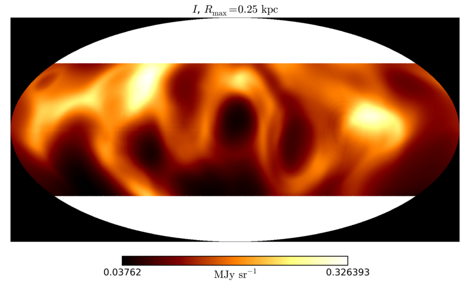
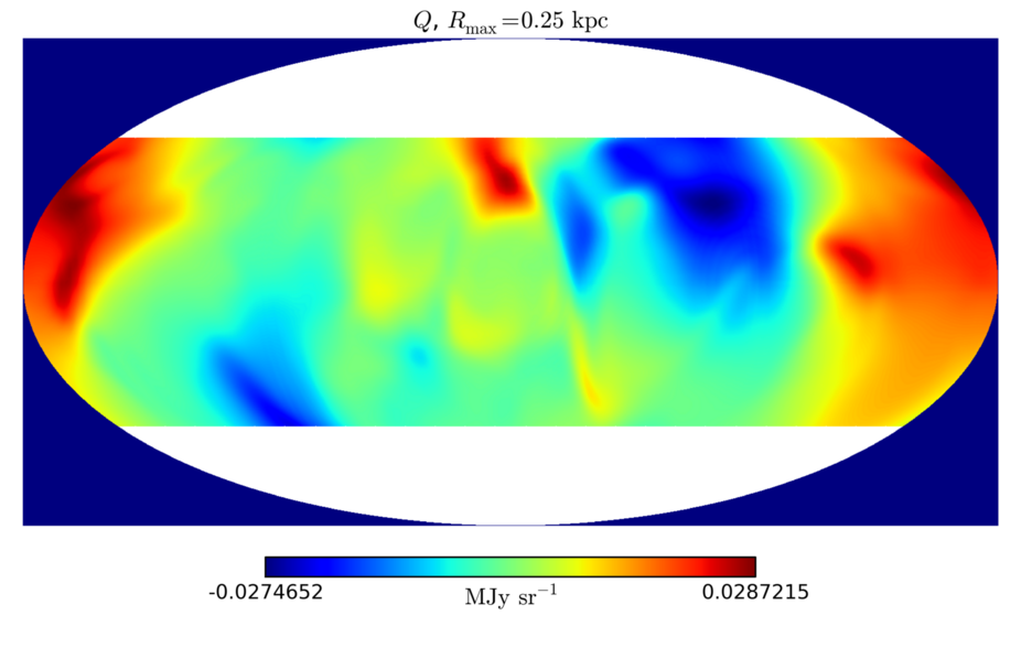
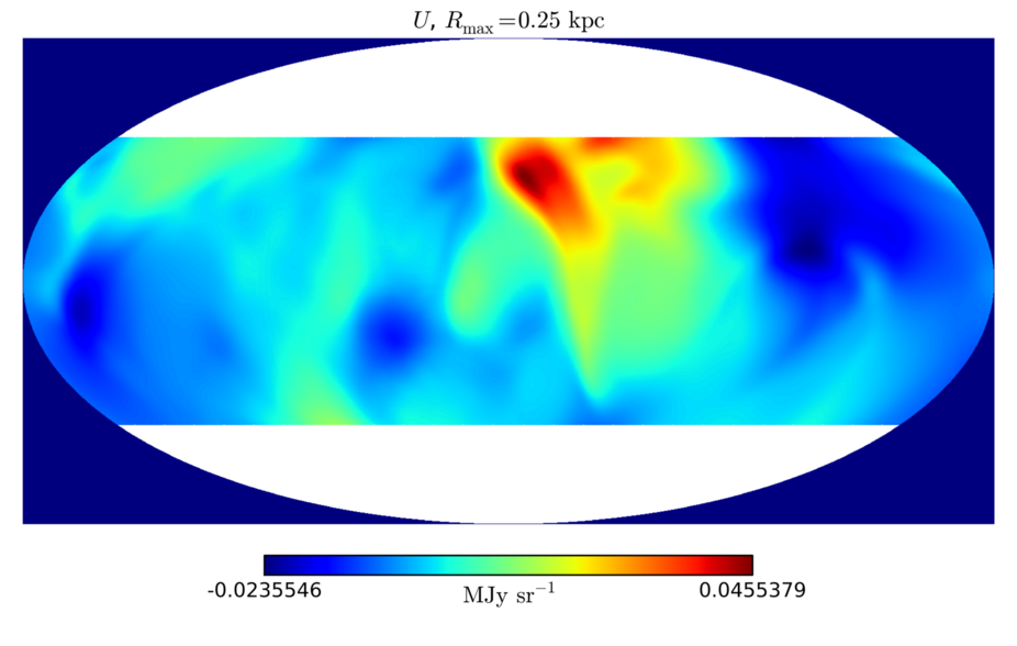
Figure 15: Stokes $I$, $Q$ and $U$ with $R_{\mathrm{max}}=0.25$ kpc.

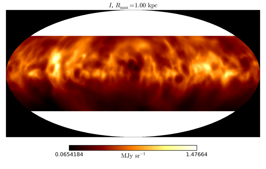
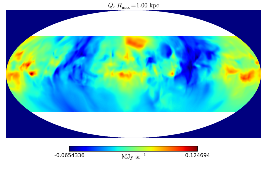
Figure 16: Stokes $I$, $Q$ and $U$ with $R_{\mathrm{max}}=1$ kpc.

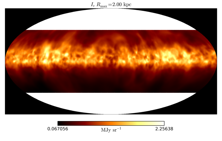
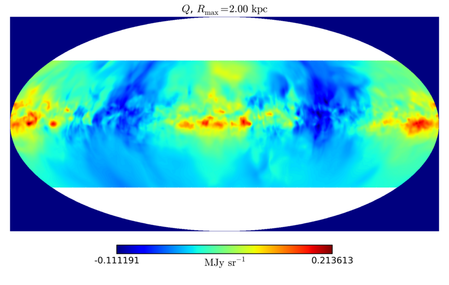
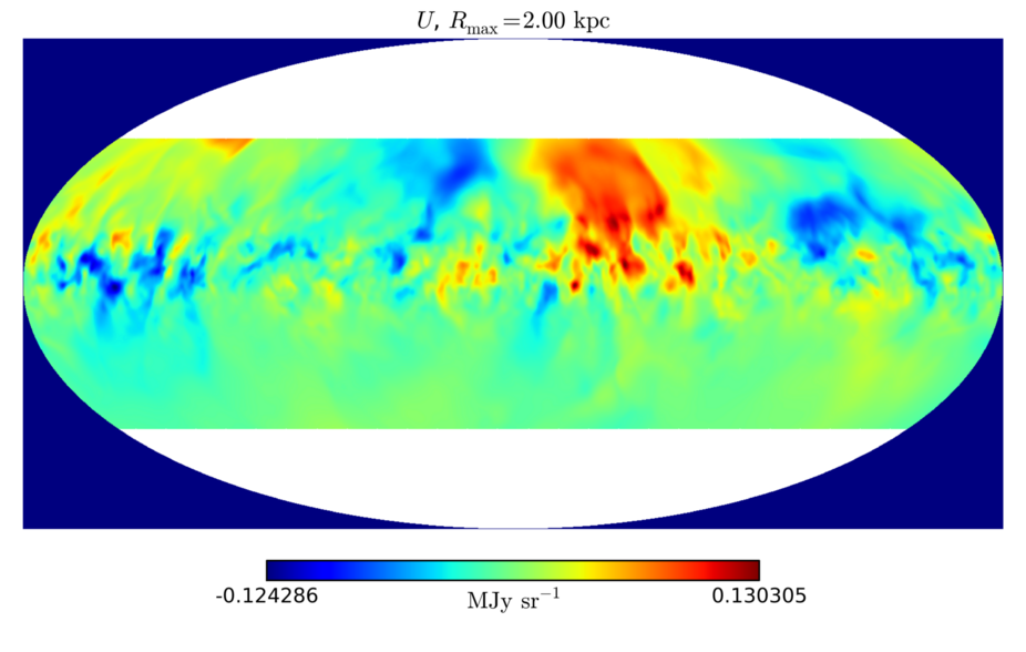
Figure 17: Stokes $I$, $Q$ and $U$ with $R_{\mathrm{max}}=2$ kpc.

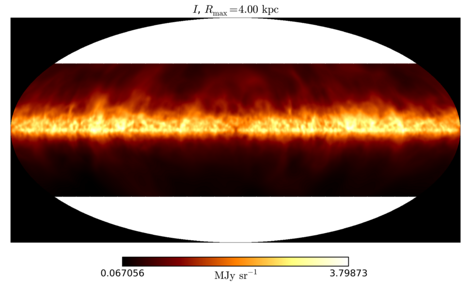
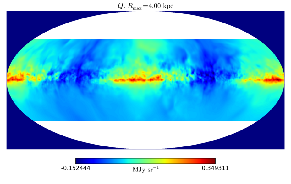
Figure 18: Stokes $I$, $Q$ and $U$ with $R_{\mathrm{max}}=4$ kpc.

Appendix B The MHD model

The focus of this paper is to explore the unique insights possible by using physically driven multiphase ISM and dynamo generated simulation magnetic field data to derive synthetic observations. These can then be compared with astronomical observations and those of simulations based on imposed flows and magnetic field configurations. We stress that the MHD simulations are not designed to model features in the ISM that have been observed or modelled by Planck or other observers, but independently to examine the multiphase structure and dynamo action of supernova driven turbulence in the ISM. These simulations have been described in detail elsewhere, but without breaking the focus on the core purpose of this paper, here we shall clarify for the reader more of the basic assumptions and techniques relating to the MHD models.

In this particular model SNe are modelled by injecting thermal and kinetic energy of 10⁵¹ erg into a spherical region, from which the pressure gradient and momentum drive shock fronts and heating into the ambient ISM. The thermal component has been found to be critical for efficient generation of vorticity through baroclinicity (Käpylä et al. 2018), and this is beneficial for dynamo action, unlike models applying momentum forcing, which are dominated by potential flows (Iffrig & Hennebelle 2017). The timing and location are motivated by observational estimates of SN distribution in the solar neighbourhood, and placement is not dependent on the local ISM density or temperature, avoiding excessive damping in dense material or the accumulation of immovable overdense regions. The environment applies an initial vertical density profile based on estimates summarized in Ferrière (2001), subject to gravitational acceleration following Kuijken & Gilmore (1989) and differentially rotating with angular speed and rotation consistent with the solar neighbourhood. The resulting turbulence, magnetic field structure, and the multiphase structure of the ISM are thus determined by the solution of the physical equations and random SN events, and not imposed. The system of equations being solved include continuity, momentum, energy and induction treating the ISM as a monatomic ideal gas

$$\frac{D\rho}{Dt} = -{\rho\@vec{\nabla}\cdot\@vec{u}}+\dot{\rho}_{\rm SN},$$

$$\frac{D\@vec{u}}{Dt} = -c_{s}^{2}\@vec{\nabla}\left(\frac{s}{c_{p}}+\textrm{ln}\rho\right)+{\@vec{g}}-Su_{x}\bm{\hat{y}}-2\@vec{\Omega}\times\@vec{u}+\frac{\@vec{j}\times\@vec{B}}{\rho}$$

$$+ \nu\@vec{\nabla}^{2}\@vec{u}+\frac{\nu}{3}\@vec{\nabla}\@vec{\nabla}\cdot\@vec{u}+2\bm{\mathsf{S}}\cdot\left(\nu\@vec{\nabla}\textrm{ln}\rho+\@vec{\nabla}\nu\right)+\zeta_{\nu}\left(\@vec{\nabla}\@vec{\nabla}\cdot\@vec{u}\right),$$

$$\rho T\frac{Ds}{Dt} = \dot{\sigma}_{\rm{SN}}+\rho\Gamma-\rho^{2}\Lambda+c_{p}\@vec{\nabla}\cdot\chi\rho\@vec{\nabla}T+2\rho\nu\bm{\mathsf{S}}^{2}$$

$$+ \rho T\@vec{\nabla}\zeta_{\chi}\cdot\@vec{\nabla}s+\mu_{0}\eta|\@vec{j}|^{2},$$

$$\frac{\partial\@vec{A}}{\partial t} = \@vec{u}\times\@vec{B}-SA_{y}\@vec{\hat{x}}-Sx\frac{\partial\@vec{A}}{\partial y}\,$$

$$+ (\eta+\zeta_{\eta})\@vec{\nabla}^{2}\@vec{A}+(\@vec{\nabla}\cdot\@vec{A})\,({{\@vec{\nabla}\eta+}}\@vec{\nabla}\zeta_{\eta}),$$

with the symbols having their usual meaning. For a full explanation refer to the earlier papers.

Modelling a galactic dynamo required an integration time in excess of 1 Gyr, with a time step below 100 yr, and on occasions less than 1 yr, with our chosen resolution of 4 pc along each edge. A lower resolution would permit faster progress with reduced resources, but careful experiments with various resolutions established 4 pc provided the minimum resolution with our numerical scheme to faithfully evolve SN remnants with the relevant essential physics (Gent 2012, Appendix A). There is a seed magnetic field of a few nG, which is amplified by the SN driven turbulence to saturate with a mean field strength a few $\mu$G. Unlike most other similar models with imposed magnetic fields and unphysical forcing, the field structure is derived from the physical processes modelled. The motivation for the 1 kpc horizontal extent was to ensure no artificial self-feedback from SN superbubbles, which can expand as far as 500 pc, and to include all estimated dynamo modes. Some similar models apply AMR with local resolution near 1 pc, although elsewhere within the models the resolution can be an order of magnitude weaker, but they are not seeking dynamo solutions. Improving the resolution four fold would multiply the size of the calculation at each iteration by $4^{3}$ and increase the number of iterations per Myr by at least $4^{2}$. A detailed analysis of the multiphase structure and properties of the ISM obtained with this model is reported in Gent et al. (2013a), and these are very consistent with results reported by other authors adopting higher resolution and employing AMR (Joung & Mac Low 2006; de Avillez & Breitschwerdt 2007; Hill et al. 2012). Other than obtaining higher maximal values for density and higher proportion of cold gas due to the enhanced resolution, the phases obtained are still similarly located and distributed, and exhibit the same temperature and velocity characteristics.

The reason for this is that the difference between 1 and 4 pc does not permit the inclusion of qualitatively distinct physics. Even a ten-fold increase in maximal densities would not bring the model within the threshold demanding self-gravity. The Jeans mass for gas at 100 cm^-3 at 100 K is $4.4\times 10^{33}$ kg. The total in a $(4{\rm pc})^{3}$ volume element is less than $10^{31}$ kg, so no regions within the model are close to being susceptible to gravitational instability, and this would be the case even for models with ten times more dense regions. The typical cooling times in our MHD model are about 100 yr, but occasionally as low as 1 yr, never sufficiently dense to introduce unresolved thermal instabilities, which lead to cloud collapse and these processes are also absent for models with 1 pc resolution. Even where isolated regions within such models may approach the critical Jeans mass, they are unlikely to have enough significance to the global dynamics to justify the numerical overheads.

Increased resolution is, of course, desirable, but comes with a numerical cost. Higher resolution would increase the Reynolds numbers applicable in the model, permitting smaller magnetic and velocity structures to be resolved and perhaps more efficient dynamo action. For further illustrations, including video representations, of the simulation data see http://fagent.wikidot.com/astro.

References

- Abbott (1982) Abbott, D. C. 1982, ApJ, 263, 723
- Alina et al. (2016) Alina, D., Montier, L., Ristorcelli, I., et al. 2016, A&A, 595, A57
- Beck (2016) Beck, R. 2016, A&A Rev., 24, 4
- Beck et al. (1996) Beck, R., Brandenburg, A., Moss, D., Shukurov, A., & Sokoloff, D. 1996, ARA&A, 34, 155
- Bendre et al. (2015) Bendre, A., Gressel, O., & Elstner, D. 2015, Astronomische Nachrichten, 336, 991
- Bethell et al. (2007) Bethell, T. J., Chepurnov, A., Lazarian, A., & Kim, J. 2007, ApJ, 663, 1055
- Chandrasekhar & Fermi (1953) Chandrasekhar, S. & Fermi, E. 1953, ApJ, 118, 113
- Chen et al. (2016) Chen, C.-Y., King, P. K., & Li, Z.-Y. 2016, ApJ, 829, 84
- Chevalier (1977) Chevalier, R. A. 1977, ARA&A, 15, 175
- Davis (1951) Davis, L. 1951, Phys. Rev., 81, 890
- de Avillez & Breitschwerdt (2007) de Avillez, M. A. & Breitschwerdt, D. 2007, ApJ, 665, L35
- Draine & Weingartner (1996) Draine, B. T. & Weingartner, J. C. 1996, ApJ, 470, 551
- Elmegreen & Scalo (2004) Elmegreen, B. G. & Scalo, J. 2004, ARA&A, 42, 211
- Evirgen et al. (2017) Evirgen, C. C., Gent, F. A., Shukurov, A., Fletcher, A., & Bushby, P. 2017, MNRAS, 464, L105
- Evirgen et al. (2018) Evirgen, C. C., Gent, F. A., Shukurov, A., Fletcher, A., & Bushby, P. 2018, in preparation
- Falceta-Gonçalves et al. (2008) Falceta-Gonçalves, D., Lazarian, A., & Kowal, G. 2008, ApJ, 679, 537
- Ferrière (2001) Ferrière, K. M. 2001, RevModPhys, 73, 1031
- Ferrière (2001) Ferrière, K. M. 2001, Reviews of Modern Physics, 73, 1031
- Gent (2012) Gent, F. 2012, PhD thesis, Newcastle University, http://hdl.handle.net/10443/1755
- Gent et al. (2013a) Gent, F. A., Shukurov, A., Fletcher, A., Sarson, G. R., & Mantere, M. J. 2013a, MNRAS, 432, 1396
- Gent et al. (2013b) Gent, F. A., Shukurov, A., Sarson, G. R., Fletcher, A., & Mantere, M. J. 2013b, MNRAS, 430, L40
- Gordon et al. (2017) Gordon, K. D., Baes, M., Bianchi, S., et al. 2017, A&A, 603, A114
- Gressel (2010) Gressel, O. 2010, PhD thesis, PhD Thesis, 2010
- Haverkorn (2015) Haverkorn, M. 2015, in Magnetic Fields in Diffuse Media, ed. A. Lazarian, E. M. de Gouveia Dal Pino, & C. Melioli (Berlin: Springer), 483
- Heiles (1996) Heiles, C. 1996, ApJ, 462, 316
- Hennebelle et al. (2008) Hennebelle, P., Banerjee, R., Vázquez-Semadeni, E., Klessen, R. S., & Audit, E. 2008, A&A, 486, L43
- Hennebelle & Iffrig (2014) Hennebelle, P. & Iffrig, O. 2014, A&A, 570, A81
- Hildebrand et al. (2009) Hildebrand, R. H., Kirby, L., Dotson, J. L., Houde, M., & Vaillancourt, J. E. 2009, ApJ, 696, 567
- Hill et al. (2012) Hill, A. S., Joung, M. R., Mac Low, M. M., et al. 2012, ApJ, 750, 104
- Hollins et al. (2017) Hollins, J. F., Sarson, G. R., Shukurov, A., Fletcher, A., & Gent, F. A. 2017, ApJ, 850, 4
- Houde et al. (2009) Houde, M., Vaillancourt, J. E., Hildebrand, R. H., Chitsazzadeh, S., & Kirby, L. 2009, ApJ, 706, 1504
- Iffrig & Hennebelle (2017) Iffrig, O. & Hennebelle, P. 2017, A&A, 604, A70
- Joung & Mac Low (2006) Joung, M. K. R. & Mac Low, M.-M. 2006, ApJ, 653, 1266
- Juvela (2005) Juvela, M. 2005, A&A, 440, 531
- Käpylä et al. (2018) Käpylä, M. J., Gent, F. A., Väisälä, M. S., & Sarson, G. R. 2018, A&A, 611, A15
- Kim & Ostriker (2015) Kim, C.-G. & Ostriker, E. C. 2015, ApJ, 815, 67
- Klein & Fletcher (2015) Klein, U. & Fletcher, A. 2015, Galactic and Intergalactic Magnetic Fields
- Kuijken & Gilmore (1989) Kuijken, K. & Gilmore, G. 1989, MNRAS, 239, 605
- Lamarre et al. (2010) Lamarre, J.-M., Puget, J.-L., Ade, P. A. R., et al. 2010, A&A, 520, A9
- Lozinskaya (1992) Lozinskaya, T. A. 1992, Supernovae and stellar wind in the interstellar medium
- Mac Low et al. (2005) Mac Low, M.-M., Balsara, D. S., Kim, J., & de Avillez, M. A. 2005, ApJ, 626, 864
- Mathis et al. (1983) Mathis, J. S., Mezger, P. G., & Panagia, N. 1983, A&A, 128, 212
- McKee & Ostriker (1977) McKee, C. F. & Ostriker, J. P. 1977, ApJ, 218, 148
- Montier et al. (2015) Montier, L., Plaszczynski, S., Levrier, F., et al. 2015, A&A, 574, A135
- Ostriker et al. (2001) Ostriker, E. C., Stone, J. M., & Gammie, C. F. 2001, ApJ, 546, 980
- Padoan et al. (2001) Padoan, P., Goodman, A., Draine, B. T., et al. 2001, ApJ, 559, 1005
- Pelkonen et al. (2009) Pelkonen, V.-M., Juvela, M., & Padoan, P. 2009, A&A, 502, 833
- Planck Collaboration I (2011) Planck Collaboration I. 2011, A&A, 536, A1
- Planck Collaboration I (2016) Planck Collaboration I. 2016, A&A, 594, A1
- Planck Collaboration Int. XIX (2015) Planck Collaboration Int. XIX. 2015, A&A, 576, A104
- Planck Collaboration Int. XLII (2016) Planck Collaboration Int. XLII. 2016, A&A, 596, A103
- Planck Collaboration Int. XLIV (2016) Planck Collaboration Int. XLIV. 2016, A&A, 596, A105
- Planck Collaboration Int. XX (2015) Planck Collaboration Int. XX. 2015, A&A, 576, A105
- Planck Collaboration Int. XXI (2015) Planck Collaboration Int. XXI. 2015, A&A, 576, A106
- Planck Collaboration Int. XXII (2015) Planck Collaboration Int. XXII. 2015, A&A, 576, A107
- Planck Collaboration Int. XXXII (2016) Planck Collaboration Int. XXXII. 2016, A&A, 586, A135
- Planck Collaboration Int. XXXIII (2016) Planck Collaboration Int. XXXIII. 2016, A&A, 586, A136
- Planck Collaboration Int. XXXV (2016) Planck Collaboration Int. XXXV. 2016, A&A, 586, A138
- Planck Collaboration X (2016) Planck Collaboration X. 2016, A&A, 594, A10
- Rand & Kulkarni (1989) Rand, R. J. & Kulkarni, S. R. 1989, ApJ, 343, 760
- Soler et al. (2016) Soler, J. D., Alves, F., Boulanger, F., et al. 2016, A&A, 596, A93
- Soler et al. (2013) Soler, J. D., Hennebelle, P., Martin, P. G., et al. 2013, ApJ, 774, 128
- Steenbeck et al. (1966) Steenbeck, M., Krause, F., & Rädler, K.-H. 1966, Zeitschrift Naturforschung Teil A, 21, 369
- Tammann et al. (1994) Tammann, G. A., Löffler, W., & Schröder, A. 1994, ApJS, 92, 487
- Vazquez-Semadeni (1994) Vazquez-Semadeni, E. 1994, ApJ, 423, 681
- Zubko et al. (2004) Zubko, V., Dwek, E., & Arendt, R. G. 2004, ApJS, 152, 211