Non-canonical Conformal Attractors for Single Field Inflation

Abstract

We extend the idea of conformal attractors in inflation to non-canonical sectors by developing a non-canonical conformally invariant theory from two different approaches. In the first approach, namely, ${\cal N}=1$ supergravity, the construction is more or less phenomenological, where the non-canonical kinetic sector is derived from a particular form of the Kähler potential respecting shift symmetry. In the second approach i.e., superconformal theory, we derive the form of the Lagrangian from a superconformal action and it turns out to be exactly of the same form as in the first approach. Conformal breaking of these theories results in a new class of non-canonical models which can govern inflation with modulated shape of the T-models. We further employ this framework to explore inflationary phenomenology with a representative example and show how the form of the Kähler potential can possibly be constrained in non-canonical models using the latest confidence contour in the $n_{s}-r$ plane given by recent Planck and BICEP/Keck results.

1 Introduction

The idea of spontaneous conformal/superconformal symmetry breaking in inflation [2, 1, 3] explains meticulously how different class of inflationary models can make very similar observational predictions, even though their formulations are entirely different and their potentials are apparently uncorrelated. Examples include Starobinsky model [4], chaotic inflation with $\lambda\phi^{4}$ potential and non-minimal coupling to gravity $\frac{\xi}{2}\phi^{2}R$ ($\xi>0$) [5], Higgs inflation with $\xi<0$ [6] among others. With the advantage of this mechanism one can also propose new class of inflationary models [3] which form a universality class and in terms of observational data they all have an attractor point in the leading order approximation and these class of models are termed as conformal attractors.

The scheme of these conformal attractors is the following: One starts with at least two real scalar fields. The first one is the good old inflaton field $\phi$ that is responsible for inflationary dynamics. The second one(s) is(are) a conformal field(s) $\chi$, called conformon. These so-called conformons are conformally coupled to gravity and usually their kinetic terms are canonical, albeit with opposite sign. In addition, the potential terms consist of an $SO(1,1)$ symmetry breaking arbitrary function $F(\frac{\phi}{\chi})$ and the total action has a local conformal symmetry. However, as is well-known, the theory of inflation should not be conformally invariant. So, the way one can make inflation happen in the attractor framework is to choose a particular gauge and break the conformal symmetry in such a way that conformal field(s) get(s) decoupled from the theory. Thus the spontaneous symmetry breaking of conformal invariance results in a functional choice of the potential of the form $F(\tanh\frac{\psi}{\sqrt{6}})$ in Einstein frame in terms of the canonically normalized field $\psi$. Depending upon the functional choice of the potential one will end up with different models such as Starobinsky, chaotic T-models [3], etc. Further, in order to realize inflation in terms of observational data, one notices that all of these models have an attractor point given by : $1-n_{s}=\frac{2}{N_{e}}$, $r=\frac{12}{N_{e}^{2}}$ in the leading order approximation in $1/N_{e}$, where $N_{e}$ is the number of e-folding of inflation. Hence the name conformal attractors. Thus, in this common framework, idea of conformal attractors explain how different, apparently uncorrelated, inflationary models end up with identical observational predictions. A superconformal version of the attractor scenario can further accommodate complex scalar fields as well but the rest of the mechanism remains the same [7]. This notion has further been been extended to multiple-field inflation scenario [8], non-minimal inflationary attractors [9], and all of these models further been generalized to $\alpha$-attractor models [10, 11]. The major success of these $\alpha$-attractor models are that one can arrive at different inflationary models from a single Lagrangian, depending upon the different values of a single parameter $\alpha$ in the theory. In these class of models, kinetic term is non-canonical and it has an overall co-efficient $\alpha$. But in the potential term this parameter $\alpha$ may or may not appear, as it is rather a matter of choice. As a result the value of tensor-to-scalar ratio $r$ is proportional to $\alpha$ and the scalar spectral index $n_{s}$ is independent of it.

What is common among the above models is that, barring $\alpha$-attractors, all the other models deal with canonical fields. However, conformal breaking of non-canonical fields have not been well-investigated for till date. In fact, there are very few examples in the literature where some non-canonical conformal invariance from some particular superconformal theories have been studied, but eventually some specific choices have made kinetic terms canonical [12, 13, 2]. So, proper development of conformal attractor scenario for non-canonical fields is in need. On the other hand, non-canonical models of inflation have particularly become important in the light of recent observational data. As Planck 2015 and Planck 2018 confirmed some scale-dependence in the power spectrum at 5-$\sigma$ [14, 15], non-canonical models, from which one can in general generate scale-dependent power spectrum have become more relevant than ever. So, this is quite timely one does a thorough study of non-canonical conformal attractors by investigating for proper conformal breaking of non-canonical models. The primary intention of the present article is to extend the idea of conformal attractors to generic class of non-canonical models of the inflation and to see if there is any superconformal realization of the setup, finally leading to a demonstration of inflationary phenomenology in the light of latest observations from Planck 2015, 2018 and BICEP/Keck [14, 15, 16]. In the process, we will also demonstrate how one can reproduce canonical conformal attractors for particular choice of the parameters from this generic framework.

In this article, our approach is quite generic and straightforward. First, we will start from a rather general form of the non-minimal K$\ddot{a}$hler potential of $\mathcal{N}=1$ supergravity which is invariant under shift symmetry. We will then choose a particular superpotential phenomenologically, derive the non-canonical action therefrom, make this action conformally invariant by adding necessary terms into the theory. We will then employ this K$\ddot{a}$hler potential and superpotential to derive a generic action for inflation. Next, we will engage ourselves in demonstrating how one can derive this apparently phenomenological action from superconformal approach. Having establishing a proper superconformal framework for the action, we will then develop the non-canonical conformal attractor scenario using this action, resulting in a generic inflaton potential. This generic potential is found to have parametric choices for which the height of the T-model potentials is increasing. The possible reason being higher order terms of non-homogeneous non-canonical kinetic term of the theory. Finally we employ the above framework to demonstrate briefly, with a representative example, inflationary phenomenology in the light of latest observational data from Planck 2015, 2018, BICEP/Keck [14, 15, 16]. We also study its phenomenological implications therefrom and show how one can constrain the K$\ddot{a}$hler potential from observations.

2 Basic phenomenological setup

Let us start with a Kähler potential of the form

$$K=-\left[\sum_{\begin{subarray}{c}n=1\end{subarray}}^{l}K^{(n)}\left(\Phi^{n}-\Phi^{*n}\right)\right]^{2}+SS^{*}-\zeta(SS^{*})^{2}$$ (2.1)

Here $\Phi$ is the chiral superfield which plays the roll of inflation and $K^{(n)}$ are dimensionless coupling constants of their self interactions. One can notice that this Kähler potential is invariant under the following shift transformation;

$$\sum_{\begin{subarray}{c}n=1\end{subarray}}^{l}K^{(n)}\Phi^{n}\rightarrow\sum_{\begin{subarray}{c}n=1\end{subarray}}^{l}K^{(n)}\Phi^{n}+C^{N}$$ (2.2)

This shift symmetry rather generalizes the shift symmetries proposed in [17, 18, 19]. Due to this shift symmetry Eq.(2.2), one can consider the term $\sum_{\begin{subarray}{c}n=1\end{subarray}}^{l}K^{(n)}\Phi^{n}$ as a composite field $\hat{\Phi}$ and the real component of this composite field $\hat{\Phi}$, will be absent in the Kähler potential Eq.(2.1). Hence, the real component of $\hat{\Phi}$, i.e., $\text{Re}\left[\sum_{\begin{subarray}{c}n=1\end{subarray}}^{l}K^{(n)}\Phi^{n}\right]=\text{Re}\left[\hat{\Phi}\right]$ can be identified as the inflaton scalar field. This is to avoid the usual $\eta$-problem[20]. However, physics is invariant under field transformation, one can also continue the same analysis in terms of the non-canonical variable $\Phi$ of the Kähler potential Eq.(2.1). So, in such a scenario, real part of $\Phi$ can be identified as inflaton, see the refs [19, 18] for further clarifications.

The chiral multiplet $S$ plays the roll of an auxiliary field and it attains a zero vev at the time of inflation. The term $SS^{*}$ gives the required potential to the $\Phi$ field. In absence of this, by considering the nature of supergravity potential and the nature of shift symmetry in the K$\ddot{a}$hler potential, the potential will not be bounded from the below[17]. However, if we only consider $SS^{*}$ during inflation, this field creates tachyonic instability by acquiring a mass much smaller than the Hubble scale, resulting in the production of inflationary fluctuations and these fluctuations will be added to the source of isocurvature perturbations or to the source of non-Gaussian adiabatic perturbations [21]. This problem can be evaded by adding the term $\zeta(SS^{*})^{2}$ to Eq.(2.1), so that the mass of the $S$ field will become greater than the Hubble scale and the corresponding fluctuations of $S$ will not be generated. Thus this term ensures the stability of inflationary trajectory near $S=0$. Once the stabilization is achieved, the field $S$ vanishes and this term becomes irrelevant after inflation. As the stabilizer field plays a crucial roll in the construction of supergravity inflation, people have investigated the nature of this field. The roll of a stabilizer field in supergravity inflation and its stabilization issues has been discussed and explained in detail in [17, 22, 23, 24, 12, 13]. Some recent proposals to identify this as an sGoldstino, a supersymmetric scalar partner of goldstino fermion can be found in [23]. Alternatively, one can also propose a framework to replace stabilizer field by nilpotent superfields in the K$\ddot{a}$hler potential [25, 26]. We will, however, consider the widely accepted stabilizer field approach.

The Kähler potential defined in Eq.(2.1) can give the following kinetic term for inflation:

$$\frac{1}{\sqrt{-g}}L_{kin}=-2\left[\sum_{\begin{subarray}{c}n=1\end{subarray}}^{l}K^{(n)}n\Phi^{n-1}\sum_{\begin{subarray}{c}n=1\end{subarray}}^{l}K^{(n)}n\Phi^{*n-1}\right]\\ \times\partial_{\mu}\Phi\partial^{\mu}\Phi^{*}-\left(1-4\zeta S^{*}S\right)\partial_{\mu}S\partial^{\mu}S^{*}$$ (2.3)

By decomposing $\Phi$ in terms of real and imaginary components $\Phi=\frac{1}{\sqrt{2}}\left(\phi+i\chi\right)$, and by assuming along flat direction $S=\chi_{i}=0$, the Eq.(2.3) can be written as

$$\frac{1}{\sqrt{-g}}L_{kin}=-\left[\sum_{\begin{subarray}{c}n=1\end{subarray}}^{l}\frac{K^{(n)}n}{\left(\sqrt{2}\right)^{n-2}}\phi^{n-1}\right]^{2}\frac{1}{2}\partial_{\mu}\phi\partial^{\mu}\phi$$ (2.4)

This can be further written more simply in the form

$$\frac{1}{\sqrt{-g}}L_{kin}=-\left[\sum_{\begin{subarray}{c}n=1\end{subarray}}^{l}l^{(n)}\phi^{n-1}\right]^{2}\frac{1}{2}\partial_{\mu}\phi\partial^{\mu}\phi$$ (2.5)

with $l^{(n)}=\frac{K^{(n)}n}{\left(\sqrt{2}\right)^{n-2}}$. After squaring the series this can be written in more abstract form as

$$\frac{1}{\sqrt{-g}}L_{kin}=-\sum_{\begin{subarray}{c}n=1\end{subarray}}^{2l-1}g^{(n)}\phi^{n-1}\frac{1}{2}\partial_{\mu}\phi\partial^{\mu}\phi$$ (2.6)

In terms of new index $h$ this series can be written in more convenient form as

$$\frac{1}{\sqrt{-g}}L_{kin}=-\sum_{\begin{subarray}{c}h=2\end{subarray}}^{2l}K^{(h)}\phi^{h-2}\frac{1}{2}\partial_{\mu}\phi\partial^{\mu}\phi$$ (2.7)

Here $K^{(h)}$ is related to $g^{(n)}$ by $K^{(h)}=g^{(h-1)}$. Now for a superpotential of the form

$$W=S\left[\sum_{\begin{subarray}{c}h=2\end{subarray}}^{2l}\left(K^{(h)}\sqrt{2}^{h}\Phi^{h}\right)^{2}\right]^{1/2}$$ (2.8)

can generate the F-term potential of the form

$$V=\sum_{\begin{subarray}{c}h=2\end{subarray}}^{2l}\left(K^{(h)}\phi^{h}\right)^{2}$$ (2.9)

Thus the total Lagrangian using Eq.(2.7) and Eq.(2.9) takes the form

$$L=\sqrt{-g}\left[\frac{R}{2}-\sum_{\begin{subarray}{c}h=2\end{subarray}}^{2l}K^{(h)}\phi^{h-2}\frac{1}{2}\partial_{\mu}\phi\partial^{\mu}\phi-\sum_{\begin{subarray}{c}h=2\end{subarray}}^{2l}\left(K^{(h)}\Phi^{h}\right)^{2}\right]$$ (2.10)

In order to build a theory for conformal breaking of this non-canonical field $\phi$, we have to add necessary terms to the Lagrangian: first, this field $\phi$ should be conformally coupled to $R$ and secondly, we have to add the conformon field $\chi$ to the Lagrangian in an equal footing with the $\phi$ field in kinetic term and in coupling to $R$ term. By adding these terms and including corresponding potential term for conformon field in Eq.(2.10), one can write this Lagrangian in Jordan frame as

$$L^{J}=\sqrt{-g}\sum_{h=2}^{2l}\left[\frac{C^{(h)}\chi^{h-2}}{2}\partial_{\mu}\chi\partial^{\mu}\chi+\frac{C^{(h)}\chi^{h}}{3h^{2}}R-\frac{K^{(h)}\phi^{h-2}}{2}\partial_{\mu}\phi\partial^{\mu}\phi\right.\\ \left.-\frac{K^{(h)}\phi^{h}}{3h^{2}}R-\frac{4}{9h^{4}}F\left(\frac{\phi}{\chi}\right)(K^{(h)}\phi^{h}-C^{(h)}\chi^{h})^{2}\right]$$ (2.11)

where $C^{(h)}$ is the dimensionless coupling constants for the interactions of conformal field $\chi$. Here the term $F\left(\frac{\phi}{\chi}\right)$ have been added to confirm quasi de Sitter evolution after the conformal breaking [3]. Thus this construction Eq.(2.11) seems to be purely phenomenological since it is well known that the Poincaŕe supergravity theories have the lack of conformon fields. Note that for $2l=2$ this Lagrangian Eq.(2.11) boils down to the conformal invariant Lagrangian with canonical kinetic terms, which is used to study the construction of conformal attractors [3]. Compared to this canonical conformal attractors [3] what we are doing is that by adding more higher order terms into the conformal attractors, we here explicitly breaking the conformal symmetry of the same. But one can notice that the Lagrangian Eq.(2.11) has a conformal symmetry if one avoids the summation in $h$ index, under the following set of transformations

$$g^{{}^{\prime}}_{\mu\nu}=e^{-2\sigma(x)}g_{\mu\nu},~{}~{}~{}~{}~{}~{}~{}~{}\chi^{{}^{\prime}}=e^{\frac{2}{h}\sigma(x)}\chi,~{}~{}~{}~{}~{}~{}~{}~{}\phi^{{}^{\prime}}=e^{\frac{2}{h}\sigma(x)}\phi.$$ (2.12)

But this observation is irrelevant in the present discussion, but what we claim is that one can pass through this kind of Lagrangian Eq.(2.11) from a superconformal approach when the second conformal field $\eta$ is decouples from the theory, which we will show in the next section.

3 Superconformal realization of the setup

In the last section, we have given a phenomenological framework to construct a Lagrangian defined in Eq.(2.11) required for the study of conformal breaking of non-canonical fields. In this section we will demonstrate how the above Lagrangian Eq.(2.11) can be derived from the superconformal action. For this purpose, let us start our calculation by considering two complex scalar conformons $X_{1}^{0}$ and $X_{2}^{0}$, in the K$\ddot{a}$hler embedding manifold ${\cal N}(X,\bar{X})$ along with scalar superfield $X^{1}=\Phi$ as inflaton and an sGoldstino $X^{2}=S$ as a stabilizer field. In terms of this embedding K$\ddot{a}$hler potential $\cal N$, general superconformal action for scalar-gravity part is defined [7] as

$$\frac{1}{\sqrt{-g}}{\cal L}_{sc}^{\rm scalar-grav}=-\frac{1}{6}{\cal N}(X,\bar{X})R-G_{I\bar{J}}{\cal D}^{\mu}X^{I}{\cal D}_{\mu}\bar{X}^{\bar{J}}-G^{I\bar{J}}{\cal W}_{I}\bar{\cal W}_{\bar{J}}$$ (3.1)

where ${\cal W}(X)$ is the superpotential and $G_{I\bar{J}}$ is the K$\ddot{a}$hler metric which is defined as

$$G_{I\bar{J}}\equiv\frac{\partial^{2}{\cal N}}{\partial X^{I}\partial\bar{X}^{\bar{J}}}$$ (3.2)

and $W_{I}\equiv\frac{\partial{\cal W}}{\partial X^{I}}$ and $\bar{W}_{\bar{J}}\equiv\frac{\partial{\cal\bar{W}}}{\partial\bar{X}^{\bar{J}}}$. For our calculations we only need to consider a local conformal invariance in Eq.(3.1) and need not bother about the other symmetries provided by the superconformal theory such as local special conformal symmetry, local $U(1)\cal R$ symmetry etc. This clearly indicate that, in this approach, we do not want to construct the potential term from the superpotential ${\cal W}(X)$. The only requirement on the potential term $V(X,\bar{X})$ to get the local conformal invariance in Eq.(3.1) is that it should be homogeneous and second degree in both $X$ and $\bar{X}$ [2] , which is stated as

$$V(X,\bar{X})=\lambda^{2}\bar{\lambda}^{2}V(X,\bar{X})$$ (3.3)

With this condition the superconformal action Eq.(3.1) becomes conformal action with the scalar-gravity Lagrangian

$$\frac{1}{\sqrt{-g}}{\cal L}_{c}^{\rm scalar-grav}=-\frac{1}{6}{\cal N}(X,\bar{X})R-G_{I\bar{J}}{\partial}^{\mu}X^{I}{\partial}_{\mu}\bar{X}^{\bar{J}}-V(X,\bar{X})$$ (3.4)

Imposing the condition Eq.(3.3) we can choose a potential of the form

$$V=\sum_{h=a+b}^{N}\frac{1}{9}F\left(\frac{X^{1}}{X_{1}^{0}}\right)\left(\frac{K^{(h)}(X^{1})^{a}(\bar{X}^{\bar{1}})^{b}}{E^{(h)}(X_{2}^{0})^{a-1}(\bar{X_{2}}^{\bar{0}})^{b-1}}-\frac{C^{(h)}(X_{1}^{0})^{a}(\bar{X_{1}}^{\bar{0}})^{b}}{E^{(h)}(X_{2}^{0})^{a-1}(\bar{X_{2}}^{\bar{0}})^{b-1}}\right)^{2}$$ (3.5)

Where $K^{(h)}$, $C^{(h)}$, and $E^{(h)}$ are the dimensionless coupling constants for the fields $X^{1}$ (inflaton superfield), $X_{1}^{0}$ (first conformon superfield)and $X_{2}^{0}$ (second conformon superfield) respectively and the values of $K^{(2)}$, $C^{(2)}$, and $E^{(2)}$ are normalized to unity. Also we consider an embedding K$\ddot{a}$hler potential manifold

$${\cal N}(X,\bar{X})=\left|S\right|^{2}-3\varsigma\frac{(S\bar{S})^{2}}{\left|X_{1}^{0}\right|^{2}-\left|X^{1}\right|^{2}}+\sum_{h=a+b}^{N}\left(\frac{K^{(h)}(X^{1})^{a}(\bar{X}^{\bar{1}})^{b}}{E^{(h)}(X_{2}^{0})^{a-1}(\bar{X_{2}}^{\bar{0}})^{b-1}}-\frac{C^{(h)}(X_{1}^{0})^{a}(\bar{X_{1}}^{\bar{0}})^{b}}{E^{(h)}(X_{2}^{0})^{a-1}(\bar{X_{2}}^{\bar{0}})^{b-1}}\right)$$ (3.6)

One can easily check that this embedding K$\ddot{a}$hler potential satisfies the following conditions

$${\cal N}(X,\bar{X})=X^{I}{\cal N}_{I}=\bar{X}^{\bar{J}}{\cal N}_{\bar{J}}=X^{I}{\cal N}_{I\bar{J}}\bar{X}^{\bar{J}}$$ (3.7)

where ${\cal N}_{I}\equiv\frac{\partial{\cal N}}{\partial X^{I}}$, and

$${\cal N}_{IK\bar{L}}X^{I}={\cal N}_{\bar{I}K\bar{L}}=0,{\cal N}_{IK\bar{L}}\bar{X}^{L}={\cal N}_{IK}$$ (3.8)

This means that ${\cal N}$ should be homogeneous and first degree in both X and $\bar{X}$, which implies

$${\cal N}(X,\bar{X})=\lambda\bar{\lambda}({\cal N}(X,\bar{X})$$ (3.9)

It has been shown in [2] that if the K$\ddot{a}$hler potential of the embedding manifold ${\cal N}(X,\bar{X})$ satisfies the conditions Eq.(3.7) and Eq.(3.8) and the potential satisfies the condition Eq.(3.3), then the action Eq.(3.4) has a local conformal invariance under the following transformations

$$g^{{}^{\prime}}_{\mu\nu}=e^{-2\sigma(x)}g_{\mu\nu},~{}~{}~{}~{}(X^{I})^{{}^{\prime}}=e^{\sigma(x)}X^{I},~{}~{}~{}~{}(\bar{X}^{\bar{J}})^{{}^{\prime}}=e^{\sigma(x)}\bar{X}^{\bar{J}}$$ (3.10)

With the advantage of this conformal symmetry Eq.(3.10), one can gauge away the conformal fields, which are responsible for negative kinetic terms, from the theory by fixing a gauge, since there are no degrees of freedom associated with these fields. The most convenient way of doing this gauge fixing is to choose a gauge which is ${\cal N}(X,\bar{X})=3$ in Eq.(3.1). This helps us to recover the standard Einstein term $-\frac{R}{2}$ of supergravity in Eq.(3.1). This gauge fixing can be interpreted as a migration from ${\cal N}=1$ superconformal theory to ${\cal N}=1$ standard Poincaŕe supergravity theory via spontaneous breaking of super conformal symmetry. However, for simplicity, we choose a gauge

$${\cal N}(X,\bar{X})=-3(N-1)$$ (3.11)

instead of choosing ${\cal N}(X,\bar{X})=3$. (We have explicitly checked that choosing and working with either of these two gauges will not altered the final inflationary predictions. If one working with the gauge ${\cal N}(X,\bar{X})=3$, then how the major equations will change is mentioned in the appendix A. There one can see that the final inflationary predictions will not change in both the gauge choices.) This dilatational gauge Eq.(3.11) can be achieved by choosing a two set of system of $N-1$ equations as follows:

$$E^{(h)}(X_{2}^{0})^{a-1}(\bar{X_{2}}^{\bar{0}})^{b-1}=\frac{h^{2}}{2}$$ (3.12)

with a condition $ab\simeq\frac{h^{2}}{4}$ and

$$C^{(h)}(X_{1}^{0})^{a}(\bar{X_{1}}^{\bar{0}})^{b}-K^{(h)}(X^{1})^{a}(\bar{X}^{\bar{1}})^{b}=\frac{3}{2}h^{2}.$$ (3.13)

We will fix the first gauge choice Eq.(3.12) in this section and the second gauge Eq.(3.13) in the next section. We show this gauge fixing in the theory explicitly in the following way: In terms of ${\cal N}(X,\bar{X})$ defined in Eq.(3.6) and in terms of potential defined in Eq.(3.5), the action Eq.(3.4) reads

$$\frac{1}{\sqrt{-g}}{\cal L}_{c}^{\rm scalar-grav}=-\frac{1}{6}\left[\sum_{h=a+b}^{N}\left(\frac{K^{(h)}(X^{1})^{a}(\bar{X}^{\bar{1}})^{b}}{E^{(h)}(X_{2}^{0})^{a-1}(\bar{X_{2}}^{\bar{0}})^{b-1}}-\frac{C^{(h)}(X_{1}^{0})^{a}(\bar{X_{1}}^{\bar{0}})^{b}}{E^{(h)}(X_{2}^{0})^{a-1}(\bar{X_{2}}^{\bar{0}})^{b-1}}\right)\right.\\ \left.+\left|s\right|^{2}-3\varsigma\frac{(s\bar{s})^{2}}{\left|X_{1}^{0}\right|^{2}-\left|X^{1}\right|^{2}}\right]R-\sum_{h=a+b}^{N}\left[-G_{I\bar{J}}{\partial}^{\mu}X^{I}{\partial}^{\mu}\bar{X}^{\bar{J}}\right.\\ \left.-\frac{1}{9}F\left(\frac{X^{1}}{X_{1}^{0}}\right)\left(\frac{K^{(h)}(X^{1})^{a}(\bar{X}^{\bar{1}})^{b}}{E^{(h)}(X_{2}^{0})^{a-1}(\bar{X_{2}}^{\bar{0}})^{b-1}}-\frac{C^{(h)}(X_{1}^{0})^{a}(\bar{X_{1}}^{\bar{0}})^{b}}{E^{(h)}(X_{2}^{0})^{a-1}(\bar{X_{2}}^{\bar{0}})^{b-1}}\right)^{2}\right]$$ (3.14)

It goes without saying that since this action has been constructed according to the conditions Eq.(3.7),Eq.(3.8) and Eq.(3.3), it has local conformal invariance under the above transformations Eq.(3.10) and the K$\ddot{a}$hler matrix $G_{I\bar{J}}$ takes the form

$$G_{I\bar{J}}\equiv\frac{\partial^{2}{\cal N}}{\partial X^{I}\partial\bar{X}^{\bar{J}}}=\begin{bmatrix}G_{0_{1}\bar{0_{1}}}&G_{0_{1}\bar{0_{2}}}&G_{0_{1}\bar{1}}&G_{0_{1}\bar{2}}\\ G_{0_{2}\bar{0_{1}}}&G_{0_{2}\bar{0_{2}}}&G_{0_{2}\bar{1}}&G_{0_{2}\bar{2}}\\ G_{1\bar{0_{1}}}&G_{1\bar{0_{2}}}&G_{1\bar{1}}&G_{1\bar{2}}\\ G_{2\bar{0_{1}}}&G_{2\bar{0_{2}}}&G_{2\bar{1}}&G_{2\bar{2}}\end{bmatrix}$$ (3.15)

We are now in a position to construct the action that we defined in Eq.(2.11). In order to do so, we will only consider the case in the above K$\ddot{a}$hler matrix $G_{I\bar{J}}$ leading to flat direction, and hence the condition is

$$G_{I\bar{J}}=\delta_{I\bar{J}}=\frac{\partial^{2}{\cal N}}{\partial X^{I}\partial\bar{X}^{\bar{J}}}$$ (3.16)

Written explicitly, the components of this flat K$\ddot{a}$hler metric are as follows:

$$G_{0_{1}\bar{0_{1}}}=\frac{\partial^{2}{\cal N}}{\partial X_{1}^{0}\partial\bar{X_{1}}^{\bar{0}}}=\sum_{h=a+b}^{N}-\frac{C^{(h)}ab(X_{1}^{0})^{a-1}(\bar{X_{1}}^{\bar{0}})^{b-1}}{E^{(h)}(X_{2}^{0})^{a-1}(\bar{X_{2}}^{\bar{0}})^{b-1}}$$ (3.17)

$$G_{0_{2}\bar{0_{2}}}=\frac{\partial^{2}{\cal N}}{\partial X_{2}^{0}\partial\bar{X_{2}}^{\bar{0}}}=\sum_{h=a+b}^{N}(1-a)(1-b)\left(\frac{K^{(h)}(X^{1})^{a}(\bar{X}^{\bar{1}})^{b}}{E^{(h)}(X_{2}^{0})^{a}(\bar{X_{2}}^{\bar{0}})^{b}}-\frac{C^{(h)}(X_{1}^{0})^{a}(\bar{X_{1}}^{\bar{0}})^{b}}{E^{(h)}(X_{2}^{0})^{a}(\bar{X_{2}}^{\bar{0}})^{b}}\right)$$ (3.18)

$$G_{1\bar{1}}=\frac{\partial^{2}{\cal N}}{\partial X^{1}\partial\bar{X}^{\bar{1}}}=\sum_{h=a+b}^{N}\frac{K^{(h)}ab(X^{1})^{a-1}(\bar{X}^{\bar{1}})^{b-1}}{E^{(h)}(X_{2}^{0})^{a-1}(\bar{X_{2}}^{\bar{0}})^{b-1}}$$ (3.19)

In terms of these components the Lagrangian Eq.(3.10) takes the form

$$\frac{1}{\sqrt{-g}}{\cal L}_{c}^{\rm scalar-grav}=\sum_{h=a+b}^{N}-\frac{1}{6}\left[\left(\frac{K^{(h)}(X^{1})^{a}(\bar{X}^{\bar{1}})^{b}}{E^{(h)}(X_{2}^{0})^{a-1}(\bar{X_{2}}^{\bar{0}})^{b-1}}-\frac{C^{(h)}(X_{1}^{0})^{a}(\bar{X_{1}}^{\bar{0}})^{b}}{E^{(h)}(X_{2}^{0})^{a-1}(\bar{X_{2}}^{\bar{0}})^{b-1}}\right)R\right.\\ \left.+\frac{C^{(h)}ab(X_{1}^{0})^{a-1}(\bar{X_{1}}^{\bar{0}})^{b-1}}{E^{(h)}(X_{2}^{0})^{a-1}(\bar{X_{2}}^{\bar{0}})^{b-1}}\partial^{\mu}X_{1}^{0}\partial_{\mu}\bar{X}_{1}^{\bar{0}}-\frac{K^{(h)}ab(X^{1})^{a-1}(\bar{X}^{\bar{1}})^{b-1}}{E^{(h)}(X_{2}^{0})^{a-1}(\bar{X_{2}}^{\bar{0}})^{b-1}}\partial^{\mu}X^{1}\partial_{\mu}\bar{X}^{\bar{1}}\right.\\ \left.-(1-a)(1-b)\left(\frac{K^{(h)}(X^{1})^{a}(\bar{X}^{\bar{1}})^{b}}{E^{(h)}(X_{2}^{0})^{a}(\bar{X_{2}}^{\bar{0}})^{b}}-\frac{C^{(h)}(X_{1}^{0})^{a}(\bar{X_{1}}^{\bar{0}})^{b}}{E^{(h)}(X_{2}^{0})^{a}(\bar{X_{2}}^{\bar{0}})^{b}}\right)\partial^{\mu}X_{2}^{0}\partial_{\mu}\bar{X}_{2}^{\bar{0}}\right.\\ \left.-\frac{1}{9}F\left(\frac{X^{1}}{X_{1}^{0}}\right)\left(\frac{K^{(h)}(X^{1})^{a}(\bar{X}^{\bar{1}})^{b}}{E^{(h)}(X_{2}^{0})^{a-1}(\bar{X_{2}}^{\bar{0}})^{b-1}}-\frac{C^{(h)}(X_{1}^{0})^{a}(\bar{X_{1}}^{\bar{0}})^{b}}{E^{(h)}(X_{2}^{0})^{a-1}(\bar{X_{2}}^{\bar{0}})^{b-1}}\right)^{2}\right]$$ (3.20)

Here we have not written the terms associated with the stabilizer field as we know that this field attains zero vev during inflation. If we assume the fields are real during inflation (corresponding partners are stabilized at zero during inflation)

$$X_{1}^{0}=\bar{X}_{1}^{\bar{0}}=\frac{\chi}{\sqrt{2}},~{}~{}~{}~{}X_{2}^{0}=\bar{X}_{2}^{\bar{0}}=\frac{\eta}{\sqrt{2}},~{}~{}~{}~{}~{}X^{1}=\bar{X}^{\bar{1}}=\frac{\phi}{\sqrt{2}}$$ (3.21)

then the Lagrangian Eq.(3.20) in terms of these real fields looks

$${\cal L}_{c}^{\rm scalar-grav}=\sqrt{-g}\sum_{h=a+b=2}^{N}\left\{-\frac{R}{12}\left(\frac{K^{(h)}\phi^{h}}{E^{(h)}\eta^{h-2}}-\frac{C^{(h)}\chi^{h}}{E^{(h)}\eta^{h-2}}\right)+\frac{C^{(h)}ab}{2E^{(h)}}\left(\frac{\chi}{\eta}\right)^{h-2}\partial^{\mu}\chi\partial_{\mu}\chi\right.\\ \left.-\frac{K^{(h)}ab}{2E^{(h)}}\left(\frac{\phi}{\eta}\right)^{h-2}\partial^{\mu}\phi\partial_{\mu}\phi-\frac{(1-a)(1-b)}{2E^{(h)}}\left[K^{(h)}\left(\frac{\phi}{\eta}\right)^{h}-C^{(h)}\left(\frac{\chi}{\eta}\right)^{h}\right]\partial^{\mu}\eta\partial_{\mu}\eta\right.\\ \left.-\frac{1}{36}F\left(\frac{\phi}{\chi}\right)\left(\frac{K^{(h)}\phi^{h}}{E^{(h)}\eta^{h-2}}-\frac{C^{(h)}\chi^{h}}{E^{(h)}\eta^{h-2}}\right)^{2}\right\}$$ (3.22)

In the process, we gauge away the second conformal field $\eta$ from the above theory by fixing the gauge Eq.(3.12), and in terms of the real field $\eta$ this gauge has the form:

$$E^{(h)}\eta^{h-2}=\frac{h^{2}}{4}$$ (3.23)

with an additional condition $ab\simeq\frac{h^{2}}{4}$, (a term $\sqrt{2}^{h}$ in the denominator of left hand side of Eq.(3.23) has removed since it will cancel out with the gauge Eq.(3.13).) and Eq.(3.22) then takes the form

$$L=\sqrt{-g}\sum_{h=a+b=2}^{N}\left[\left(\frac{C^{(h)}\chi^{h}}{3h^{2}}-\frac{K^{(h)}\phi^{h}}{3h^{2}}\right)R+\frac{C^{(h)}\chi^{h-2}}{2}\partial_{\mu}\chi\partial^{\mu}\chi-\frac{K^{(h)}\phi^{h-2}}{2}\partial_{\mu}\phi\partial^{\mu}\phi\right.\\ \left.-\frac{4}{9h^{4}}F\left(\frac{\phi}{\chi}\right)(K^{(h)}\phi^{h}-C^{(h)}\chi^{h})^{2}\right]$$ (3.24)

The resulting equation above exactly matches the erstwhile supergravity derived phenomenological model Eq.(2.11) proposed in the previous section under the identifications $N=2l$. Thus we end up with a Lagrangian which contains non-canonical non-homogeneous kinetic terms for both conformal field $\chi$ and for inflaton field $\phi$ with an equal footing, after the decoupling of the second conformal field $\eta$ from the superconformal action. Now the role of this second conformal field $X_{2}^{0}=\frac{\eta}{2}$ is clear, which helps us to maintain the conformal symmetry in the theory when one essentially wants to deal with a non-canonical non-homogeneous kinetic term for the conformal field $\chi$.

4 Single field non-canonical conformal attractors

Having convinced ourselves about the theoretical framework, let us now employ this scenario in proposing conformal attractor framework for non-canonical fields. For this, we start from the Lagrangian proposed earlier in Eq.(2.11). From the superconformal scenario, we have seen that this Lagrangian is a conformal broken one after the gauge fixing of second conformon field $\eta$. Also from the superconformal point of view that we have discussed in the previous section, this Lagrangian has an enhanced conformal symmetry when $N=2$ case, which is canonical and this case has studied in details in [3] and known as conformal attractors. For reader’s convenience again we recall the Lagrangian Eq.(2.11) here

$$\begin{split}L^{J}=\sqrt{-g}\sum_{h=2}^{N}\left[\frac{C^{(h)}\chi^{h-2}}{2}\partial_{\mu}\chi\partial^{\mu}\chi+\frac{C^{(h)}\chi^{h}}{3h^{2}}R-\frac{K^{(h)}\phi^{h-2}}{2}\partial_{\mu}\phi\partial^{\mu}\phi\right.\\ \left.-\frac{K^{(h)}\phi^{h}}{3h^{2}}R-\frac{4}{9h^{4}}F\left(\frac{\phi}{\chi}\right)\left(K^{(h)}\phi^{h}-C^{(h)}\chi^{h}\right)^{2}\right]\end{split}$$ (4.1)

Even though this Lagrangian has decoupled from second conformal field $\eta$, one can expect some kind of symmetry in presence of the first conformon field $\chi$. As we stated earlier, we observe that this Lagrangian has a conformal symmetry if one avoids the summation in $h$ index under the transformation Eq.(2.12). Now, we will gauge away the first conformal compensator field $\chi$ from the theory using Eq.(3.13), and in terms of the real fields this gauge choice Eq. (3.13) becomes

$$C^{(h)}\chi^{h}-K^{(h)}\phi^{h}=\frac{3}{2}h^{2}$$ (4.2)

Here the term $\sqrt{2}^{h}$ in the denominator of left hand side of Eq.(4.2) has cancelled with the gauge choice Eq.(3.12) in Eq.(3.22). Resolving this constraint Eq.(4.2) in terms of canonically normalized fields $\psi_{h-1}$, one gets

$$\chi=\left[\frac{3h^{2}}{2C^{(h)}}\right]^{\frac{1}{h}}\cosh^{\frac{2}{h}}\left(\frac{\psi_{h-1}}{\sqrt{6}}\right)$$ (4.3)

and

$$\phi=\left[\frac{3h^{2}}{2K^{(h)}}\right]^{\frac{1}{h}}\sinh^{\frac{2}{h}}\left(\frac{\psi_{h-1}}{\sqrt{6}}\right)$$ (4.4)

In terms of this newly redefined canonically normalized fields $\psi_{h-1}$ the original Lagrangian Eq.(4.1) can be expressed in Einstien frame as follows:

$$L^{E}=\sum_{h=2}^{N}\sqrt{-g}\left[\frac{R}{2}-\frac{1}{2}\partial_{\mu}\psi_{h-1}\partial^{\mu}\psi_{h-1}-F\left(\frac{\left[\frac{3h^{2}}{2K^{(h)}}\right]^{\frac{1}{h}}\sinh^{\frac{2}{h}}\left(\frac{\psi_{h-1}}{\sqrt{6}}\right)}{\left[\frac{3h^{2}}{2C^{(h)}}\right]^{\frac{1}{h}}\cosh^{\frac{2}{h}}\left(\frac{\psi_{h-1}}{\sqrt{6}}\right)}\right)\right]$$ (4.5)

One can readily choose $K^{(h)}=C^{(h)}$, so that the resulting Lagrangian boils down to conformal attractors for $h=2$ case:

$$L^{E}=\sum_{h=2}^{N}\sqrt{-g}\left[\frac{R}{2}-\frac{1}{2}\partial_{\mu}\psi_{h-1}\partial^{\mu}\psi_{h-1}-F\left(\tanh^{\frac{2}{h}}\left(\frac{\psi_{h-1}}{\sqrt{6}}\right)\right)\right]$$ (4.6)

From Eq.(4.4) one can easily see that each $\psi_{h-1}$ are not strictly independent, so each of these fields can be written in terms of a single field $\psi$ as

$$\psi_{h-1}=\sqrt{6}\sinh^{-1}\left[\frac{(\sqrt{6})^{\frac{h}{2}}}{h}\sqrt{\frac{2K^{(h)}}{3}}\sinh^{\frac{h}{2}}\left(\frac{\psi}{\sqrt{6}}\right)\right]$$ (4.7)

It is obvious from the above equation that finally, our framework essentially becomes an intrinsically single field model in Einstein frame. One can readily check that if one puts this field back in the Lagrangian in Einstein frame Eq.(4.6), one readily gets back a non-canonical single field model. So, we are essentially dealing with non-canonical conformal attractors, which is the primary target of this paper.

Consequently, the final Lagrangian takes the form

$$L^{E}=\sqrt{-g}\sum_{h=2}^{N}\left\{\frac{R}{2}-\frac{(\sqrt{6})^{h}K^{(h)}\sinh^{h-2}(\frac{\psi}{\sqrt{6}})\cosh^{2}(\frac{\psi}{\sqrt{6}})}{12\left[1+\frac{2(\sqrt{6})^{h}K^{(h)}}{3h^{2}}\sinh^{h}(\frac{\psi}{\sqrt{6}})\right]}\partial_{\mu}\psi\partial^{\mu}\psi\right.\\ \left.-F\left(\tanh^{\frac{2}{h}}\left[\sinh^{-1}\left[\frac{(\sqrt{6})^{\frac{h}{2}}}{h}\sqrt{\frac{2K^{(h)}}{3}}\sinh^{\frac{h}{2}}\left(\frac{\psi}{\sqrt{6}}\right)\right]\right]\right)\right\}$$ (4.8)

It is interesting to check that for $N=2$ and for $K^{(2)}=1$ in Eq.(4.8), model becomes canonical and reduces to the result obtained in [3] whereas for any other choice this gives rise to non-canonical conformal attractors. Thus, one can get back canonical conformal attractors for particular choice of the parameters from this generic framework. This framework thus generalizes the conformal attractors as well. Also for $N=2$ and for $K^{(2)}=1$ in Eq.(4.8), functional form of the potential becomes $F(\tanh\frac{\psi}{\sqrt{6}})$, and the simplest functional choice of the potential is $\tanh^{2n}(\frac{\psi}{\sqrt{6}})$ and these are well- known T-models [3] and it has been shown in the Fig.(1(a)), where the shape of these models symmetric in nature. But in our case we have to consider $N\geq 2$ in Eq.(4.8), and for the functional choice of the potential in Eq.(4.8) we choose the form of the potential as follows:

$$V(\psi)=\lambda_{n}\sum_{h=2}^{N}\left(\tanh^{\frac{2}{h}}\left[\sinh^{-1}\left[\frac{(\sqrt{6})^{\frac{h}{2}}}{h}\sqrt{\frac{2K^{(h)}}{3}}\sinh^{\frac{h}{2}}\left(\frac{\psi}{\sqrt{6}}\right)\right]\right]\right)^{2n^{{}^{\prime}}}.$$ (4.9)

Again one can note that this potential reduces to T-model for $N=2$ and for $K^{(2)}=1$ in Eq.(4.9). As we are interested to consider the effects on non-canonical fields i.e., $N\geq 2$ in Eq.(4.8), we consider the same in the following: one can see that in the Fig.(1(b)) (In this figure all coupling constants in the potentials taken as unity for comparison and simplicity which shows how this potential behaves depending upon the different values of $N$.) the height of the potential Eq.(4.9) is increasing as the value of $N$ is increasing, i.e., as the non-canonicity of the model is increasing then the height of the potential is also increasing. But if one incorporate the effects of coupling constants in the potential Eq.(4.9) instead of treating all $K^{(h)}=1$, one can see that the stretching in the potentials is slightly modulated and stretching of potential is occurring for very large values of $\psi$, which is evidenced from the Fig.(1(c)). Moreover, one can observe that from the Fig.(1(d)), if one fixes the non-canonicity of the model, say for $N=3$, the same broadening of the potential occurring as the values of $n^{{}^{\prime}}$ increasing as in the case of canonical T-models. As a conclusion, in [3] it has been shown that switching from Jordan frame to Einstein frame in these class of conformal models causes the exponential stretching of moduli space and as a result exponential flattening of scalar potentials occur even if these potentials are very steep in the Jordan frame. Same is happening here in the case of non-canonical fields also which is evidenced from the Fig.(1).

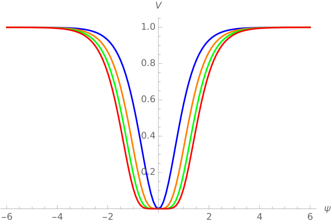
(a) T-Model potentials Eq.(4.9) for $N=2$, $n^{{}^{\prime}}=1,2,3,4$ (blue, orange, green and red respectively.), and $\lambda_{n^{{}^{\prime}}}=1$, which is proposed in [3].

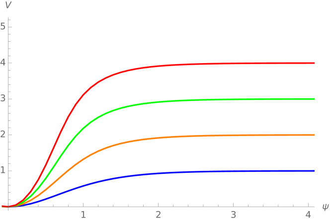
(b) Behaviour of potential Eq.(4.9) in the first quadrant, for different values of $N=2,3,4,5$ (blue, orange, green and red respectively.) for $\lambda_{n^{{}^{\prime}}}=1$, $n^{{}^{\prime}}=1$ and here also we choose all $K^{(h)}=1$ for comparison.

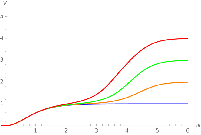
(c) Effects of coupling constants $K^{(h)}$ on the potential Eq.(4.9) in the first quadrant, for different values of $N=2,3,4,5$ (blue, orange, green and red are respectively.) for $\lambda_{n^{{}^{\prime}}}=1$, $n^{{}^{\prime}}=1$ and for arbitrary values of $K^{(2)}=1$, $K^{(3)}=0.0000082$, $K^{(4)}=0.0000006$, $K^{(5)}=0.0000002$

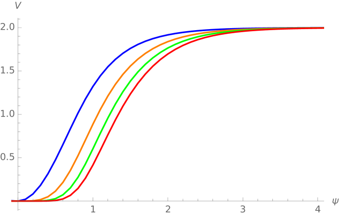
(d) Behaviour of non-canonical T-model potentials Eq.(4.9) in the first quadrant for $N=3$, $n^{{}^{\prime}}=1,2,3,4$ (blue, orange, green and red respectively.). Here we have chosen coupling constants $\lambda_{n}$ and $K^{(h)}$ are unity just for comparison and simplicity.

Figure 1: Figure depicts the potential defined in Eq.(4.9) for different cases.

5 Inflationary phenomenology

Let us now employ the above framework to demonstrate briefly, with a representative example, inflationary phenomenology in the light of latest observational data from Planck 2018 and BICEP/Keck [15, 16]. We will start with the particular functional choice of the potential of the form proposed in Eq.(4.9). In what follows will mostly concentrate on the example of super-Planckian fields $\psi>>1$ for which the potential Eq.(4.9), and subsequently, the Lagrangian Eq.(4.8) can be approximated as

$$L^{E}\simeq\sqrt{-g}\left\{\frac{R}{2}(N-1)-\left[1+\beta\left(1+4e^{-\sqrt{\frac{2}{3}}\psi}\right)\right]\frac{1}{2}\partial_{\mu}\psi\partial^{\mu}\psi-\lambda_{n}\left[(N-1)-4n^{{}^{\prime}}e^{-\sqrt{\frac{2}{3}}\psi}\right]\right\}$$ (5.1)

with

$$\beta=\frac{N(N+1)(2N+1)-30}{24}$$ (5.2)

Now one may wonder why in this approximation suddenly the coupling constants disappear from the theory. We here remind the readers that our attempt is only to study the non-canonical effects and not to study the effects of coupling constants and not to constrain the values of these coupling constants from the observation. Even though we neglect the effects of coupling constant in the leading approximation, we can still study the effects of non-canonical fields in these theories. After all these approximations, we can still see in the Eq.(5.1) the values of $N$ plays the crucial roll in the dynamics and this $N\geq 2$ value strictly represents the non-canonicity in the theory.

By varying the action Eq.(5.1) with respect to $\psi$, one can find the equation of motion for inflaton field and at the slow-roll regime this field equation takes the form

$$\left[1+\beta\left(1+4e^{-\sqrt{\frac{2}{3}}\psi}\right)\right]3H\dot{\psi}=-V_{\psi}$$ (5.3)

In terms of the large e-folding number $N_{e}$, this field equation can be further expressed as

$$\frac{d\psi}{dN_{e}}=\frac{4n^{{}^{\prime}}}{1+\beta}\sqrt{\frac{2}{3}}\frac{1}{(N-1)}e^{-\sqrt{\frac{2}{3}}\psi}$$ (5.4)

Therefore the slow-roll parameters

$$\epsilon=\frac{1}{2}\frac{1}{F(\psi)}\left(\frac{V_{\psi}}{V}\right)^{2}=\frac{3\alpha}{4N_{e}^{2}}$$ (5.5)

and

$$\eta=\epsilon+\frac{1}{2\epsilon}\frac{d\epsilon}{dN_{e}}\simeq-\frac{1}{N_{e}}$$ (5.6)

where $\alpha=1+\beta$ and $F(\psi)$ is the function in front of the kinetic term $1/2(\partial_{\mu}\psi)^{2}$ of the Lagrangian Eq.(5.1). It is now straightforward to calculate the observable parameters using the above slow roll parameters. In what follows, we only derive the two significant observable parameters namely, the running of spectral index $n_{s}$ and the tensor-to-scalar ratio $r$, and confront with the confidence contour given by Planck 2018 and BICEP/Keck [15, 16]. Given explicitly,

$$n_{s}=1-\frac{2}{N_{e}},~{}~{}~{}~{}~{}~{}~{}r=\frac{12\alpha}{N_{e}^{2}},$$ (5.7)

in the leading order approximation of $1/N_{e}$. From the expression Eq.(5.2), it is clear that $\alpha=1+\beta$ can only take the values $\alpha=1,3.25,7.25,\dots$ for the models $N=2,3,4,\dots$, respectively. The values of $n_{s}$ and $r$, as calculated for various choice of the model parameter $N$, and also for the choice of different number of e-foldings ${N_{e}=50}$ and ${N_{e}=60}$ , have been summarized in the Table (1) and (2) respectively. The allowed regions for those parameters have subsequently been analyzed vis-à-vis the confidence contours from latest observational data in Fig.(2).

Sr.no	$N$	$n_{s}$	$r$
1	2	0.96	0.0048
2	3	0.96	0.0156
3	4	0.96	0.0348
4	5	0.96	0.0648
5	6	0.96	0.108

Table 1: Values of $n_{s}$ and $r$ for different $N$ values for number of e-foldings $N_{e}=50$

Sr.no	$N$	$n_{s}$	$r$
1	2	0.9667	0.0033
2	3	0.9667	0.0108
3	4	0.9667	0.0242
4	5	0.9667	0.045
5	6	0.9667	0.075

Table 2: Values of $n_{s}$ and $r$ for different $N$ values for number of e-foldings $N_{e}=60$

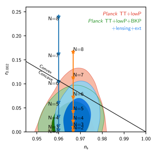
Figure 2: Comparison of the inflationary observables $n_{s}$ and $r$ for the theory Eq.(5.1) for various values of $N$ with three different confidence contours : (i) Planck TT + low P (red contours), (ii) + BKP (green contours), and (iii) + lensing + ext (blue contours). The blue line corresponds to the number of e-foldings $N_{e}=50$ and orange line corresponds to the number of e-folding $N_{e}=60$. The first star on the very bottom of the orange line represents $N=2$ case, which is the attractor point proposed in [3].

From Fig.(2) it is evident that for the number of e-folding $N_{e}=60$ (orange line), the values of $n_{s}$ from the model fall beyond the 1-$\sigma$ Planck bound for $N\geq 6$. This means that in the non-canonical sector of the theory Eq.(4.8) terms up to $N=5$ are allowed. Inclusion of higher order powers of the $\psi$ in the non-canonical sector will lead to a tension with Planck at 1-$\sigma$, of course, for this particular choice of the potential Eq.(4.9). In other words, when one consider the conformal breaking of non-canonical fields the terms up to $2l=N=5$ are relevant in the theory Eq.(2.11) for the corresponding functional choice of the potential $V=\left(\frac{\phi}{\chi}\right)^{2n}.$ Similarly in the case of number of e-foldings $N_{e}=50$ (blue line in the Fig.(2)), the same analysis can be done and it is evidenced that up to $N=5$ is also allowed. Thus, one can, in principle, constrain the form of non-canonical kinetic sector from the observation for the functional choice of the potential defined in Eq.(4.8), so as to constrain the form of Kähler potential defined in Eq.(3.6),where the value of $N$ is allowed up to 5 in this particular case.

But recent data release from BICEP/Keck gives the bounds on the tensor to scalar ratio $r$ [16]: $r_{0.05}<0.036$ at $95\%$ confidence. On behalf of this result one can strengthen the bounds on the non-canonicity of the model Eq.(4.8) and the value of $N$ is constrained only up to $N\leq 4$ for both the number of e-foldings $N_{e}=50$ and $N_{e}=60$, which is evidenced from the table Table (1) and Table (2).

6 Summary and Outlook

In this article we have developed a non-canonical generalization of the class of conformal models with universal attractor behaviour and have also established a superconformal realization of the same. We found that in this generalization these class of models the height of the T-model potential is increasing due to the non-canonical terms in the original conformal theory. It turns out that exponential flattening of potential at the boundary of moduli space is occurring, when the fields switch from Jordan frame to Einstein frame though gauge fixing is violated partially due to the same non-canonical terms.

We have also engaged ourselves in finding out the phenomenological consequences of these non-canonical conformal attractors via a representative example for inflation. By confronting the values of two significant observable parameters, namely, the running of scalar spectral index $n_{s}$ and the tensor-to-scalar ratio $r$, with the confidence contour in the $n_{s}-r$ plane as given by Planck 2018 and recent BICEP/Keck, we tried to put certain constraints on the form of the K$\ddot{a}$hler potential from observations. It turned out that, for our particular potential under consideration, in the non-canonical sector of the theory only up to $N=4$ (according to recent BICEP/Keck results [16]) terms are allowed when one considers number of e-foldings $N_{e}=60$ and the higher order terms in $\phi$ have to be thrown away from the kinetic sector due to observational constraints. This mechanism thus helps us put certain constraints on the erstwhile arbitrary Kähler potential from observations.

As $\alpha$-attractor models are generalized version of conformal attractors, it is expected that our analysis for non-canonical conformal attractors should, in principle, be generalized to non-canonical $\alpha$-attractors as well. It is also interesting to investigate if our single field inflation approach can be extended to multi-field inflation models as well and the possible consequences therefrom [27]. Further, as has been shown in a recent interesting paper [28], the $\alpha$-attractor framework can be employed to study late time phenomena like dark matter and dark energy models. In the same vein, it would be interesting to see the possible consequences of these non-canonical attractors in late time universe. We hope to address some of these issues in near future.

Appendix A ${\cal N}(X,\bar{X})=3$ gauge

If one works with the gauge ${\cal N}(X,\bar{X})=3$ instead of working with Eq.(3.11), the major changes are listed below:

Eq.(4.2) will be modified as

$$C^{(h)}\chi^{h}-K^{(h)}\phi^{h}=\frac{3}{2(N-1)}h^{2}$$ (A.1)

Resolving this constraint in terms of canonically normalized fields $\psi$, one gets

$$\chi=\left[\frac{3h^{2}}{2C^{(h)}(N-1)}\right]^{\frac{1}{h}}\cosh^{\frac{2}{h}}\left(\frac{\psi_{h-1}}{\sqrt{6}}\right)$$ (A.2)

and

$$\phi=\left[\frac{3h^{2}}{2K^{(h)}(N-1)}\right]^{\frac{1}{h}}\sinh^{\frac{2}{h}}\left(\frac{\psi_{h-1}}{\sqrt{6}}\right)$$ (A.3)

Now Eq.(2.11) reads in Einstein frame as

$$L^{E}=\sum_{h=2}^{N}\frac{\sqrt{-g}}{(N-1)}\left[\frac{R}{2}-\frac{1}{2}\partial_{\mu}\psi_{h-1}\partial^{\mu}\psi_{h-1}-\frac{1}{(N-1)}F\left(\frac{\left[\frac{3h^{2}}{2K^{(h)}}\right]^{\frac{1}{h}}\sinh^{\frac{2}{h}}\left(\frac{\psi_{h-1}}{\sqrt{6}}\right)}{\left[\frac{3h^{2}}{2C^{(h)}}\right]^{\frac{1}{h}}\cosh^{\frac{2}{h}}\left(\frac{\psi_{h-1}}{\sqrt{6}}\right)}\right)\right]$$ (A.4)

If one chooses $K^{(h)}=C^{(h)}$, the resulting Lagrangian boils down as

$$L^{E}=\sum_{h=2}^{N}\frac{\sqrt{-g}}{(N-1)}\left[\frac{R}{2}-\frac{1}{2}\partial_{\mu}\psi_{h-1}\partial^{\mu}\psi_{h-1}-\frac{1}{(N-1)}F\left(\tanh^{\frac{2}{h}}\left(\frac{\psi_{h-1}}{\sqrt{6}}\right)\right)\right]$$ (A.5)

$\psi_{h-1}$ fields can be written in terms of a single field $\psi$ as

$$\psi_{h-1}=\sqrt{6}\sinh^{-1}\left[\frac{(\sqrt{6})^{\frac{h}{2}}}{h(N-1)^{\frac{h-2}{4}}}\sqrt{\frac{2K^{(h)}}{3}}\sinh^{\frac{h}{2}}\left(\frac{\psi}{\sqrt{6}}\right)\right]$$ (A.6)

Consequently, the Lagrangian Eq.(A.5) takes the form

$$L^{E}=\sqrt{-g}\sum_{h=2}^{N}\left\{\frac{R}{2(N-1)}-\frac{(\sqrt{6})^{h}K^{(h)}\sinh^{h-2}(\frac{\psi}{\sqrt{6}})\cosh^{2}(\frac{\psi}{\sqrt{6}})}{12(N-1)^{\frac{h}{2}}\left[1+\frac{2(\sqrt{6})^{h}K^{(h)}}{3h^{2}(N-1)^{\frac{h}{2}}}\sinh^{h}(\frac{\psi}{\sqrt{6}})\right]}\partial_{\mu}\psi\partial^{\mu}\psi\right.\\ \left.-\frac{1}{(N-1)^{2}}F\left(\tanh^{\frac{2}{h}}\left[\sinh^{-1}\left[\frac{(\sqrt{6})^{\frac{h}{2}}}{h(N-1)^{\frac{h-2}{4}}}\sqrt{\frac{2K^{(h)}}{3}}\sinh^{\frac{h}{2}}\left(\frac{\psi}{\sqrt{6}}\right)\right]\right]\right)\right\}$$ (A.7)

We choose the following potential instead of Eq.(4.9)

$$V(\psi)=\frac{\lambda_{n}}{(N-1)^{2}}\sum_{h=2}^{N}\left(\tanh^{\frac{2}{h}}\left[\sinh^{-1}\left[\frac{(\sqrt{6})^{\frac{h}{2}}}{h(N-1)^{\frac{h-2}{4}}}\sqrt{\frac{2K^{(h)}}{3}}\sinh^{\frac{h}{2}}\left(\frac{\psi}{\sqrt{6}}\right)\right]\right]\right)^{2n^{{}^{\prime}}}.$$ (A.8)

For large values of $\psi>>1$ one can approximate the final Lagrangian for the Eq.(A.7) and Eq(A.8) as follows:

$$L^{E}\simeq\sqrt{-g}\left\{\frac{R}{2}-\left[1+\beta\left(1+4e^{-\sqrt{\frac{2}{3}}\psi}\right)\right]\frac{1}{2}\partial_{\mu}\psi\partial^{\mu}\psi-\frac{\lambda_{n}}{(N-1)}\left[1-\frac{4n^{{}^{\prime}}}{(N-1)}e^{-\sqrt{\frac{2}{3}}\psi}\right]\right\}$$ (A.9)

Slow-roll equation motion for the inflaton is

$$\left[1+\beta\left(1+4e^{-\sqrt{\frac{2}{3}}\psi}\right)\right]3H\dot{\psi}=-V_{\psi}$$ (A.10)

In terms of the large e-folding number $N_{e}$, this field equation can be further expressed as

$$\frac{d\psi}{dN_{e}}=\frac{4n^{{}^{\prime}}}{1+\beta}\sqrt{\frac{2}{3}}\frac{1}{(N-1)}e^{-\sqrt{\frac{2}{3}}\psi}$$ (A.11)

Therefore the slow-roll parameter $\epsilon$ becomes

$$\epsilon=\frac{1}{2}\frac{1}{F(\psi)}\left(\frac{V_{\psi}}{V}\right)^{2}=\frac{3\alpha}{4N_{e}^{2}}$$ (A.12)

This is same as that of the expression Eq.(5.5). So the rest of the inflationary analysis are same as that of the main section (5) . So, it is quiet evidenced that working with the any of these two gauges will not alter the final inflationary predictions.

References

- [1] R. Kallosh and A. D. Linde , Superconformal generalizations of the Starobinsky model, JCAP 1306 (2013) 028, [ arXiv:1306.3214 [hep-th]]
- [2] R. Kallosh and A. Linde, Superconformal Generalization of the Chaotic Inflation Model , JCAP 1306 (2013) 027, [arXiv:1306.3211 [hep-th]]
- [3] R. Kallosh and A. Linde, Universality Class in Conformal Inflation, JCAP 1307 (2013) 002, [arXiv:1306.5220 [hep-th]]
- [4] A.A. Starobinsky, A new type of isotropic cosmological models without singularity, Phys. Lett. B 91, 99(1980)
- [5] D. S. Salopek, J. R. Bond, J. M. Bardeen, Designing density fluctuation spectra in inflation, Phys. Rev. D 40, 1753 (1989)
- [6] F.L. Bezrukov and M.E. Shaposhnikov, The Standard Model Higgs boson as the inflaton, Phys.Lett.B659:703-706,2008 [arXiv:0710.3755 [hep-th]]
- [7] R. Kallosh, L. Kofman, A. Linde, A. V. Proeyen, Superconformal Symmetry, Supergravity and Cosmology, Class.Quant.Grav.17:4269-4338,2000; Erratum-ibid.21:5017,2004, [arXiv:hep-th/0006179]
- [8] R. Kallosh and A. Linde, Multi-field Conformal Cosmological Attractors, JCAP 1312 (2013) 006, [arXiv:1309.2015 [hep-th]]
- [9] R. Kallosh and A. Linde, Non-minimal Inflationary Attractors, JCAP 1310 (2013) 033 [arXiv:1307.7938 [hep-th]]
- [10] R. Kallosh, A. Linde, D. Roest, Superconformal Inflationary -Attractors, JHEP 1311 (2013) 198, [arXiv:1311.0472 [hep-th]]
- [11] R. Kallosh and A. Linde Planck, LHC, and -attractors, Phys. Rev. D 91, 083528 (2015). [arXiv:1502.07733 [astro-ph.CO]]
- [12] S. Ferrara, R. Kallosh, A. Linde, A. Marrani, A. V. Proeyen, Jordan Frame Supergravity and Inflation in NMSSM, Phys.Rev.D82:045003,2010, [arXiv:1004.0712 [hep-th]]
- [13] S. Ferrara, R. Kallosh, A. Linde, A. Marrani, A. V. Proeyen, Superconformal Symmetry, NMSSM, and Inflation, Phys.Rev.D83:025008,2011, [arXiv:1008.2942 [hep-th]]
- [14] Planck 2015 results. XIII. Cosmological parameters, Astron.Astrophys. 594 (2016) A13, [arXiv:1502.01589 [astro-ph.CO]]
- [15] Planck Collaboration, Y. Akrami et al., Planck 2018 results. X. Constraints on inflation, [ arXiv:1807.06211 [astro-ph.CO]]
- [16] BICEP, Keck Collaboration, P. A. R. Ade et al., Improved Constraints on Primordial Gravitational Waves using Planck, WMAP, and BICEP/Keck Observations through the 2018 Observing Season, Phys. Rev. Lett. 127 no. 15, (2021), [arXiv:2110.00483 [astro-ph.CO]]
- [17] M. Kawasaki, M. Yamaguchi, T. Yanagida, Natural Chaotic Inflation in Supergravity, Phys.Rev.Lett. 85 (2000) 3572-3575, [arXiv:hep-ph/0004243]
- [18] F. Takahashi, Linear Inflation from Running Kinetic Term in Supergravity , Phys.Lett. B693 (2010) 140-143, [arXiv:1006.2801 [hep-ph]]
- [19] K. Nakayama and F. Takahashi, Running Kinetic Inflation, JCAP 1011 (2010) 009, [arXiv:1008.2956 [hep-ph]]
- [20] M. Yamaguchi, Supergravity based inflation models: a review, Class.Quant.Grav. 28 (2011) 103001, [arXiv:1101.2488 [astro-ph.CO]]
- [21] S. C. Davis and M. Postma, SUGRA chaotic inflation and moduli stabilisation, JCAP0803:015,2008, [arXiv:0801.4696 [hep-ph]]
- [22] K. Das and K. Dutta, N-flation in Supergravity, Phys.Lett. B738 (2014) 457-463, [arXiv:1408.6376 [hep-ph]]
- [23] R. Kallosh, A. Linde, T. Rube, General inflaton potentials in supergravity, Phys.Rev.D83:043507,2011, [arXiv:1011.5945 [hep-th]]
- [24] V. Demozzi, A. Linde, V. Mukhanov, Supercurvaton, JCAP 1104 (2011) 013 [arXiv:1012.0549 [hep-th]]
- [25] S. Ferrara, R. Kallosh, A. Linde, Cosmology with Nilpotent Superfields, JHEP 1410 (2014) 143 , [arXiv:1408.4096 [hep-th]]
- [26] R. Kallosh and A. Linde, Inflation and Uplifting with Nilpotent Superfields, JCAP 1501 (2015) 025, [arXiv:1408.5950 [hep-th]]
- [27] T. Pinhero and S. Pal, A New Class of Non-canonical Conformal Attractors for Multi-field Inflation, [arXiv:1810.12712 [hep-th]], JCAP 2003 (2020) no.03, 022
- [28] S. S. Mishra, V. Sahni and Y. Shtanov, Sourcing Dark Matter and Dark Energy from -attractors [arXiv:1703.03295[gr-qc]]