Universality for critical heavy-tailed network models:
Metric structure of maximal components

Abstract.

We study limits of the largest connected components (viewed as metric spaces) obtained by critical percolation on uniformly chosen graphs and configuration models with heavy-tailed degrees. For rank-one inhomogeneous random graphs, such results were derived by Bhamidi, van der Hofstad, Sen (2018) [BHS15]. We develop general principles under which the identical scaling limits as in [BHS15] can be obtained. Of independent interest, we derive refined asymptotics for various susceptibility functions and the maximal diameter in the barely subcritical regime.

1. Introduction

Over the last decades, applications arising from complex systems in different fields have inspired a host of models for networks as well as models of dynamically evolving networks. One of the major themes in the study of these models has been in the nature of the emergence of the giant component. A classical example is the percolation process, where each edge of the network is independently kept with probability $p$, and deleted otherwise. As $p$ increases from 0 to 1, the graph experiences a transition in the connectivity structure, i.e., there exists a "critical percolation value" $p_{c}$ such that for any $\varepsilon>0$ and $p<p_{c}(1-\varepsilon)$, the proportion of vertices in the largest component is asymptotically negligible, while for $p>p_{c}(1+\varepsilon)$, a unique giant component emerges containing an asymptotically positive proportion of vertices [ABS04, F07, RGCN1, J09, JLR00].

Understanding the behavior at criticality is one of the key questions in statistical physics because the components exhibit unique and key features in the critical regime. In the physics literature, the critical behavior of percolation relates to studying optimal paths in networks in the so-called strong disorder regime. A wide array of conjectures and heuristic deductions of the associated critical exponents can be found in [braunstein2003optimal, braunstein2007optimal, CbAH02, Halvin05]. In a nutshell, these conjectures can be described as follows:

The intrinsic nature of the critical behavior does not depend on the exact description of the model, but only on moment conditions on the degree distribution. There are two major universality classes corresponding to the critical regime and the nature of emergence of the giant depending on whether the degree distribution has asymptotically finite third moment or infinite third moment. For example, in case of power-law degree distributions (i.e., $\mathbbm{P}(D\geq x)\approx x^{-(\tau-1)}$ the precise nature of the approximation left implicit), the nature of the critical behavior depends only on the power-law degree exponent $\tau$: (a) For $\tau>4$, the maximal component sizes are of the order $n^{2/3}$ in the critical regime, whilst typical distances in these maximal connected components scale like $n^{1/3}$; (b) For $\tau\in(3,4)$, the maximal component sizes are of the order $n^{(\tau-2)/(\tau-1)}$, whilst distances scale like $n^{(\tau-3)/(\tau-1)}$.

The above conjectures have inspired a large and beautiful collection of works in probability theory. In a seminal work, Aldous [A97] provided a detailed understanding for the vector of rescaled component sizes at criticality for Erdős-Rényi random graphs, and the scaling limits for component sizes are now well understood under quite general setups in both finite third-moment [BHL10, DHLS15, H13, Jo10, NP10b, NP10a, R12] and infinite third-moment [BHL12, DHLS16, H13, Jo10] settings. We refer the reader to [Dha18, Chapter 1], [Hof17, Chapter 4] for detailed discussions about this topic. A recent and emerging direction in this literature aims at understanding the critical component structures, and distances within these components from a very general perspective. This line of work was pioneered by Addario-Berry, Broutin and Goldschmidt [ABG09], where the largest connected components were shown to converge when viewed as metric spaces (see below for exact definitions). Subsequently, [BBSX14, BBW12, BS16] have explored the universality class corresponding to [ABG09], showing that the universality in the finite third-moment setting holds not only with respect to functionals like component sizes, but also the entire metric structure. On the other hand, in the infinite third-moment setting, a recent result [BHS15] shows that the metric structure turns out to be fundamentally different. The results in [BHS15] was obtained for one fundamental random graph model (rank-one model, closely related to the Chung-Lu [CL02b, CL02] and Norros-Reittu model [BDM06]) under the assumption that the weights follow a power-law distribution. In this paper, we explore the universality class corresponding to the candidate limit law established in [BHS15]. Informally, the main contributions of this paper are as follows:

$\rhd$ Universality theorem: We establish sufficient conditions that imply convergence to the limits established in [BHS15]. This is described later in Theorem 5.2. Since we need to set up a number of constructs, a formal statement is deferred until all of these objects have been defined. We refer to Theorem 5.2 as a universality theorem because it identifies the domain of attraction of the limit laws in [BHS15]. Informally, the theorem implies that if a sequence of dynamic networks satisfies some entrance boundary conditions in the barely subcritical regime, and evolves approximately according to the multiplicative coalescent dynamics over the critical window, then the metric structure of the critical components are close to those for rank-one inhomogeneous random graphs. Theorem 5.2 is similar in spirit to [BBSX14, Theorem 3.4], but our result holds for the infinite third-moment degrees. Technically, we do not need additional restrictions as in [BBSX14, Assumption 3.3], since we compare the metric structures in the Gromov-weak topology, instead of the Gromov-Hausdorff-Prokhorov topology. The universality theorem holds under arguably optimal assumptions (see Remark 9).

$\rhd$ Critical percolation on graphs with given degrees: Our primary motivation was to analyze the critical regime for percolation on the uniform random graph model (and the closely associated configuration model) with a prescribed degree distribution that converges to a heavy-tailed degree distribution. Limit laws for the metric structure of maximal components in the critical regime are described in Theorems 2.1 and 2.2. These results are proved under Assumption 1, which is the most general set of assumptions under which the component sizes were shown to converge in [DHLS16] (see [DHLS16, Section 2 and 3] for the applicability and necessity of these assumptions).

$\rhd$ Barely subcritical regime: In order to carry out the above analysis and in particular to apply the universality theorem for percolation on configuration models, we establish refined bounds for component sizes, various susceptibility functionals, and diameters of connected components in the barely subcritical regime of the configuration model which are of independent interest; these are described in Theorems 2.3 and 2.4.

1.1. Organization of the paper

In Section 2, we describe the configuration model and critical behavior of percolation, which is the main motivation of this paper, and then describe the main results relevant to this model. Section 3 has a detailed discussion about the relevance of the results in this paper, some open problems, and an informal description of the proof ideas. We provide a full description of the limit objects and various notions of convergence of metric-space-valued random variables in Section 4. Section 5 describes and proves the general universality result. Section 6 proves results about the configuration model in the barely subcritical regime. Finally, Section LABEL:sec:proof-metric-mc combines the above estimates with a coupling of the evolution of the configuration model through the critical percolation scaling window to finish the proof of Theorem 2.1.

2. Critical percolation on the configuration model

In this section, we state our main results. In Section 2.1, we state the results about the metric structure of the largest critical percolation clusters of the configuration model. We defer full definitions of the limit objects as well as notions of convergence of measured metric spaces to Section 4. In Section 2.2, we state the results about the barely subcritical regime, and we conclude this section with an overview of the proofs in Section 2.3.

2.1. Metric structure of the critical components

The configuration model

Consider $n$ vertices labeled by $[n]:=\{1,2,...,n\}$ and a non-increasing sequence of degrees $\boldsymbol{d}=(d_{i})_{i\in[n]}$ such that $\ell_{n}=\sum_{i\in[n]}d_{i}$ is even. For notational convenience, we suppress the dependence of the degree sequence on $n$. The configuration model on $n$ vertices having degree sequence $\boldsymbol{d}$ is constructed as follows [B80, MR95]:

• Equip vertex $j$ with $d_{j}$ stubs, or half-edges. Two half-edges create an edge once they are paired. Therefore, initially we have $\ell_{n}=\sum_{i\in[n]}d_{i}$ half-edges. Pick any one half-edge and pair it with a uniformly chosen half-edge from the remaining unpaired half-edges and keep repeating the above procedure until all the unpaired half-edges are exhausted.

Let $\mathrm{CM}_{n}(\boldsymbol{d})$ denote the graph constructed by the above procedure. Note that $\mathrm{CM}_{n}(\boldsymbol{d})$ may contain self-loops or multiple edges. Let $\mathrm{UM}_{n}(\boldsymbol{d})$ denote the graph chosen uniformly at random from the collection of all simple graphs with degree sequence $\boldsymbol{d}$. It can be shown that the conditional law $\mathrm{CM}_{n}(\boldsymbol{d})$, conditioned being simple, is same as $\mathrm{UM}_{n}(\boldsymbol{d})$ (see [RGCN1, Proposition 7.15]). It was further shown in [J09c] that, if the degree distribution satisfies a finite second-moment condition (a condition which will hold in the context of this paper), then the asymptotic probability of the graph being simple converges to a positive limit.

Let us now describe the assumptions on the degree sequences. For $p>0$, define the metric space

$$\ell^{p}_{{\scriptscriptstyle\downarrow}}=\Big{\{}(x_{1},x_{2},\dots)\in\mathbb{R}^{\mathbb{N}}_{+}:x_{1}\geq x_{2}\geq\dots,\ \sum_{i}x_{i}^{p}<\infty\Big{\}},$$ (2.1)

with metric $d(\boldsymbol{x},\boldsymbol{y})=\big{(}\sum_{i}|x_{i}-y_{i}|^{p}\big{)}^{1/p}$. Fix $\tau\in(3,4)$. Throughout this paper we use the following functionals of $\tau$:

$$\alpha=1/(\tau-1),\qquad\rho=(\tau-2)/(\tau-1),\qquad\eta=(\tau-3)/(\tau-1).$$ (2.2)

Assumption 1 (Degree sequence).

For each $n\geq 1$, let $\boldsymbol{d}=\boldsymbol{d}_{n}=(d_{1},\dots,d_{n})$ be a degree sequence ($d_{i}$’s may depend on $n$, but we suppress $n$ in the notation for clarity). We assume the following about $(\boldsymbol{d}_{n})_{n\geq 1}$ as $n\to\infty$:

1. (High-degree vertices) For each fixed $i\geq 1$, $n^{-\alpha}d_{i}\to\theta_{i},$ where $\boldsymbol{\theta}=(\theta_{1},\theta_{2},\dots)\in\ell^{3}_{{\scriptscriptstyle\downarrow}}\setminus\ell^{2}_{{\scriptscriptstyle\downarrow}}$.

2. (Moment assumptions) Let $V_{n}$ be chosen uniformly from $[n]$ (independently of $\mathrm{CM}_{n}(\boldsymbol{d}))$, and $D_{n}=d_{V_{n}}$. Then $D_{n}$ converges in distribution to some positive integer-valued random variable $D$, and

   $$\frac{1}{n}\sum_{i\in[n]}d_{i}\to\mu:=\mathbbm{E}[D],\quad\frac{1}{n}\sum_{i\in[n]}d_{i}^{2}\to\mu_{2}:=\mathbbm{E}[D^{2}],\quad\lim_{K\to\infty}\limsup_{n\to\infty}n^{-3\alpha}\sum_{i=K+1}^{n}d_{i}^{3}=0.$$ (2.3)

Remark 1.

Assumption 1 is identical to [DHLS16, Assumption 1]. We refer the reader to [DHLS16, Sections 2 and 3] for discussions about the relevance and necessity of these assumptions. It was shown in [DHLS16, Section 2] that Assumption 1 is satisfied in two key settings, when (i) the degrees are taken to be an i.i.d. sample from a power-law distribution, and (ii) the degrees are chosen according to the quantiles of a power-law distribution. The first setting has been considered in [Jo10], and the latter setting has been considered for the rank-one inhomogeneous random graphs in [BHS15, BHL12].

The component sizes of $\mathrm{CM}_{n}(\boldsymbol{d})$ are known to undergo a phase transition [JL09, MR95] depending on the parameter

$$\nu_{n}=\frac{\sum_{i\in[n]}d_{i}(d_{i}-1)}{\sum_{i\in[n]}d_{i}}\to\nu=\frac{\mathbbm{E}\left[D(D-1)\right]}{\mathbbm{E}\left[D\right]}.$$ (2.4)

When $\nu>1$, $\mathrm{CM}_{n}(\boldsymbol{d})$ is supercritical in the sense that there exists a unique giant component with high probability, and when $\nu<1$, all the components have size $o(n)$ with high probability and $\mathrm{CM}_{n}(\boldsymbol{d})$ is subcritical. In this paper, when considering percolation on $\mathrm{CM}_{n}(\boldsymbol{d})$, we will always assume that

$$\nu>1,\text{ i.e. }\mathrm{CM}_{n}(\boldsymbol{d})\text{ is supercritical.}$$ (2.5)

Percolation refers to deleting each edge of a graph independently with probability $1-p$. In the case of percolation on random graphs, the deletion of edges is also independent from the underlying graph. Let $\mathrm{CM}_{n}(\boldsymbol{d},p_{n})$ and $\mathrm{UM}_{n}(\boldsymbol{d},p_{n})$ denote the graphs obtained from percolation with probability $p_{n}$ on the graphs $\mathrm{CM}_{n}(\boldsymbol{d})$ and $\mathrm{UM}_{n}(\boldsymbol{d})$, respectively. For $p_{n}\to p$, it was shown in [J09] that the critical point for the phase transition of the component sizes is $p=1/\nu$. The critical window for percolation was studied in [DHLS16, DHLS15] to obtain the asymptotics of the largest component sizes and their surplus edges. In the infinite third-moment setting, $\mathrm{CM}_{n}(\boldsymbol{d},p_{n})$ lies in the critical window when, for some $\lambda\in\mathbb{R}$,

$$p_{n}=p_{n}(\lambda)=\frac{1}{\nu_{n}}+\frac{\lambda}{n^{\eta}}+o(n^{-\eta}).$$ (2.6)

We now explain the precise meaning of convergence of components as metric spaces. Let $\mathscr{C}_{\scriptscriptstyle(i)}^{p}(\lambda)$ denote the $i$-th largest component of $\mathrm{CM}_{n}(\boldsymbol{d},p_{n}(\lambda))$. A measured metric space is a metric space equipped with a measure on the associated Borel sigma-algebra. Each component $\mathscr{C}$ can be viewed as a measured metric space with (i) the metric being the graph distance where each edge has length one; (ii) the measure being proportional to the counting measure, i.e., for any $A\subset\mathscr{C}$, the measure of $A$ is given by $\mu_{\scriptscriptstyle\mathrm{ct},i}(A)=|A|/|\mathscr{C}_{\scriptscriptstyle(i)}^{p}(\lambda)|$, where $|A|$ denotes the cardinality of $A$. For a generic measured metric space $M=(M,\mathrm{d},\mu)$ and $a>0$, $aM$ denotes the measured metric space $(M,a\mathrm{d},\mu)$. We write $\mathscr{S}_{*}$ for the space of all measured metric spaces equipped with the Gromov-weak topology (see Section 4.1) and let $\mathscr{S}_{*}^{\mathbb{N}}$ denote the corresponding product space with the accompanying product topology. For each $n\geq 1$, view $\big{(}n^{-\eta}\mathscr{C}_{\scriptscriptstyle(i)}^{p}(\lambda)\big{)}_{i\geq 1}$ as an object in $\mathscr{S}_{*}^{\mathbb{N}}$ by appending an infinite sequence of empty metric spaces after enumerating the components in $\mathrm{CM}_{n}(\boldsymbol{d},p_{n}(\lambda))$. The main results for critical percolation on the configuration model are as follows:

Theorem 2.1.

Consider $\mathrm{CM}_{n}(\boldsymbol{d},p_{n}(\lambda))$ satisfying Assumption 1, (2.5) and (2.6) for some $\lambda\in\mathbb{R}$. There exists a sequence of random measured metric spaces $(\mathscr{M}_{i}(\lambda))_{i\geq 1}$ such that on $\mathscr{S}_{*}^{\mathbb{N}}$, as $n\to\infty$,

$$\big{(}n^{-\eta}\mathscr{C}_{\scriptscriptstyle(i)}^{p}(\lambda)\big{)}_{i\geq 1}\xrightarrow{d}\big{(}\mathscr{M}_{i}(\lambda)\big{)}_{i\geq 1}.$$ (2.7)

Theorem 2.2.

Under Assumption 1, (2.5) and (2.6) for some $\lambda\in\mathbb{R}$, the convergence in (2.7) also holds for the components of $\mathrm{UM}_{n}(\boldsymbol{d},p_{n}(\lambda))$, with the identical limiting object.

Remark 2.

The limiting objects are precisely described in Section 4.6.

Remark 3.

The notion of convergence in Theorems 2.1 and 2.2 implies weak convergence of a wide array of continuous functionals with respect to the Gromov-weak topology. For example, it implies the joint convergence of the distances between an arbitrary (but fixed) number of uniformly (and independently) chosen vertices in the $i$-th largest component of $\mathrm{CM}_{n}(\boldsymbol{d},p_{n}(\lambda))$ or $\mathrm{UM}_{n}(\boldsymbol{d},p_{n}(\lambda))$.

Remark 4.

The conclusion of Theorem 2.1 holds if the measure $\mu_{\scriptscriptstyle ct,i}$ on $\mathscr{C}_{\scriptscriptstyle(i)}^{p}$ is replaced by more general measures. Indeed, define the probability measure $\mu_{w,i}:=\sum_{k\in A}w_{k}/\sum_{k\in\mathscr{C}_{\scriptscriptstyle(i)}^{p}}w_{k}$ for $A\subset\mathscr{C}_{\scriptscriptstyle(i)}^{p}$. To prove analogous results as Theorems 2.1 and 2.2 with $\mu_{w,i}$’s, we require $w_{i}$’s to satisfy some regularity conditions (see Assumption 2 below). The reason will be discussed in Remark LABEL:rem:switch-measure.

Remark 5.

The results above can be extended to the case $\mathbbm{P}(D_{n}\geq x)\sim L(x)x^{-(\tau-1)}$, where $L(\cdot)$ is a slowly-varying function. The scaling limits would be the same, however the scaling exponents will be different as observed in [DHLS16]. In particular, the width of the scaling window now turns out to be $n^{-\eta}L_{1}(n)^{2}$ (for some slowly varying $L_{1}(\cdot)$) instead of $n^{-\eta}$, and results identical to Theorem 2.1 can be obtained by scaling the distances by $n^{\eta}L_{1}(n)^{-2}$.

2.2. Mesoscopic properties of the critical clusters: barely subcritical regime

One of the main ingredients in the proof of Theorem 2.1 is a refined analysis of various susceptibility functions in the barely subcritical regime (see (2.9) below for a definition) for the percolation process. The barely subcritical and supercritical regimes correspond to regimes that are just below or above the critical window. For the percolation process under Assumption 1, barely subcritical (supercritical) behavior is observed for $p$ satisfying $n^{\eta}(p-p_{n}(0))\to-\infty$ ($n^{\eta}(p-p_{n}(0))\to\infty$), where $p_{n}(0)$ is defined in (2.6) for $\lambda=0$. These behaviors are well understood for Erdős-Rényi random graphs [JKLP93, Section 23], [Bol01, JLR00] and configuration models in the Erdős-Rényi universality class [HM12, KS08, R12]. For barely supercritical configuration models in the heavy-tailed setting, the size of the emerging giant component was obtained in [HJL16]. We provide a detailed picture about the component sizes and susceptibility functions in the subcritical regime below.

We will prove general statements about the susceptibility functions applicable not just to percolation on the configuration model, but rather to any barely subcritical configuration model. Since percolation on a configuration model yields a configuration model [F07, J09], the above yields susceptibility functions for percolation on configuration model as a special case. To set this up we need a little more notation, where each vertex in the network is associated with both degree and weight, satisfying the following assumptions:

Assumption 2 (Barely subcritical degree sequence).

Let $\boldsymbol{d}^{\prime}=(d_{1}^{\prime},\dots,d_{n}^{\prime})$ be a degree sequence and let $w_{\scriptscriptstyle(\cdot)}:[n]\mapsto\mathbb{R}$ be a non-negative weight function such that the following conditions hold:

1. Assumption 1 holds for $\boldsymbol{d}^{\prime}$ with some $\boldsymbol{c}\in\ell^{3}_{{\scriptscriptstyle\downarrow}}\setminus\ell^{2}_{{\scriptscriptstyle\downarrow}}$, and

   $$\lim_{n\to\infty}\frac{1}{n}\sum_{i\in[n]}d_{i}^{\prime}=\mu_{d},\quad\lim_{n\to\infty}\frac{1}{n}\sum_{i\in[n]}w_{i}=\mu_{w},\quad\lim_{n\to\infty}\frac{1}{n}\sum_{i\in[n]}d_{i}^{\prime}w_{i}=\mu_{d,w}.$$ (2.8)

2. $\max_{i\in[n]}w_{i}=O(n^{\alpha})$, $\sum_{i\in[n]}w_{i}^{2}=O(n)$ and $\max\Big{\{}\sum_{i\in[n]}w_{i}^{3},\sum_{i\in[n]}d_{i}^{\prime 2}w_{i},\sum_{i\in[n]}d_{i}^{\prime}w_{i}^{2}\Big{\}}=O(n^{3\alpha}).$

3. (Barely subcritical regime) The configuration model is at the barely subcritical regime, i.e., there exists $0<\delta<\eta$ and $\lambda_{0}>0$ such that

   $$\nu_{n}^{\prime}=\frac{\sum_{i\in[n]}d_{i}^{\prime}(d_{i}^{\prime}-1)}{\sum_{i\in[n]}d_{i}^{\prime}}=1-\lambda_{0}n^{-\delta}+o(n^{-\delta}).$$ (2.9)

Let $\mathscr{C}^{\prime}(j)$ denote the connected component of $\mathrm{CM}_{n}(\boldsymbol{d}^{\prime})$ containing vertex $j$, and define C_i’= {C’(i), if i ≤j,  ∀j ∈C’(i),∅, otherwise, and $\mathscr{W}_{i}=\sum_{k\in\mathscr{C}_{i}^{\prime}}w_{k}$. Define the weight-based susceptibility functions as

$$s_{r}^{\star}=\frac{1}{n}\sum_{i\geq 1}\mathscr{W}_{i}^{r}\quad\text{for }r\geq 1,\qquad s_{pr}^{\star}=\frac{1}{n}\sum_{i\geq 1}\mathscr{W}_{i}\times|\mathscr{C}_{i}^{\prime}|.$$ (2.10)

The definition in (2.2) takes care of the double counting in the definition of susceptibility functions. Also, define the weighted distance-based susceptibility as

$$\mathcal{D}_{n}^{\star}=\frac{1}{n}\sum_{i,j\in[n]}w_{i}w_{j}\mathrm{d}(i,j)\mathbbm{1}\left\{i,j\text{ are in the same connected component}\right\},$$ (2.11)

where $\mathrm{d}$ denotes the graph distance. The goal of the next result is to show that the component sizes and the susceptibility functions defined in (2.10) and (2.11) satisfy asymptotic conditions such as the entrance boundary conditions for the multiplicative coalescent [AL98]:

Theorem 2.3 (Susceptibility functions).

Under Assumption 2, as $n\to\infty$, n^-δs_2^⋆$\xrightarrow{\mathbbm{P}}$μd,w2μdλ0, & n^-δs_pr^⋆$\xrightarrow{\mathbbm{P}}$μd,wλ0,  n^-(α+δ)W_j$\xrightarrow{\mathbbm{P}}$μd,wμdλ0c_j,
n^-3α-3δ+1s_3^⋆$\xrightarrow{\mathbbm{P}}$(μd,wμdλ0)^3∑_i=1^∞c_i^3,  n^-2δD_n^⋆$\xrightarrow{\mathbbm{P}}$μd,w2μdλ02.

For a connected graph $G$, $\Delta(G)$ denotes the diameter of the graph, and for any arbitrary graph $G$, $\Delta_{\max}(G):=\max\Delta(\mathscr{C})$, where the maximum is taken over all connected components ${\mathscr{C}\subset G}$. We simply write $\Delta_{\max}$ for $\Delta_{\max}(\mathrm{CM}_{n}(\boldsymbol{d}^{\prime}))$. The asymptotics of $\Delta_{\max}$ is derived below:

Theorem 2.4 (Maximum diameter).

Under Assumption 2, as $n\to\infty$, $\mathbbm{P}(\Delta_{\max}>n^{\delta}(\log(n))^{2})\to 0$.

Remark 6.

By taking $w_{i}=1$ for all $i\in[n]$, implies that $\mathscr{W}_{i}=|\mathscr{C}_{i}|$, and thus Theorem 2.3 hold also for the usual susceptibility functions defined in terms of the component sizes (cf. [J09b]). In the proof of Theorem 2.1, we will require a more general weight function, where $w_{i}$ is taken to be the number of half-edges deleted from vertex $i$ due to percolation.

Remark 7.

Unlike Theorem 2.1, Theorems 2.3 and 2.4 yield statements about convergence in probability to constants. So, under Assumption 2, one can use the fact from [J09c] that $\liminf_{n\to\infty}\mathbbm{P}(\mathrm{CM}_{n}(\boldsymbol{d}^{\prime})\text{is simple})>0$, and thus it immediately follows that the results in Theorems 2.3 and 2.4 hold for $\mathrm{UM}_{n}(\boldsymbol{d}^{\prime})$.

2.3. Overview of the proof

We now summarize the key ideas of the proofs at a heuristic level.

Universality theorem

As discussed earlier, we first prove a universality theorem (Theorem 5.2) which roughly states that if one replaces the vertices in a rank-one inhomogeneous random graph by small metric spaces (called blobs), then the limiting metric space structure remains identical. The characterization of blobs leads to some asymptotic negligibility conditions, formally stated in Assumption 4, which simply says that the diameter of the individual blobs must be negligible compared to the typical distances in the whole graph. However, the typical distance can be cumulatively affected by the blobs, hence we get a different scaling factor for distances in Theorem 5.2 than in Theorem 5.1.

Mesoscopic or Blob-level analysis

Percolation on $\mathrm{CM}_{n}(\boldsymbol{d})$ can be viewed as a dynamic process by associating i.i.d. uniform$[0,1]$ weights $U_{e}$ to each edge $e$, and keeping $e$ if $U_{e}\leq p$. The parameter $p\in[0,1]$ can be interpreted as time. Now for $p_{n}=p_{n}(\lambda_{n})$, for some $\lambda_{n}\to-\infty$, $\mathrm{CM}_{n}(\boldsymbol{d},p_{n}(\lambda_{n}))$ lies in the barely subcritical regime and the estimates for different functionals can be obtained using Theorem 2.3. We regard the components of $\mathrm{CM}_{n}(\boldsymbol{d},p_{n}(\lambda_{n}))$ as the blobs. Under the current scaling, the blobs shrink to zero, and the edges appearing in the dynamic process between the interval $[p_{n}(\lambda_{n}),p_{n}(\lambda)]$ connecting the blobs give rise to the macroscopic structure of the largest components of $\mathrm{CM}_{n}(\boldsymbol{d},p_{n}(\lambda))$. However, the effects of the blobs on the limiting structure are reflected via different functionals, which is the reason for referring to the properties of the blobs as mesoscopic properties.

Coupling to the multiplicative coalescent

Finally, the goal is to understand the macroscopic structure formed between blobs within the time interval $[p_{n}(\lambda_{n}),p_{n}(\lambda)]$. The merging dynamics of the components between $[p_{n}(\lambda_{n}),p_{n}(\lambda)]$ can be heuristically described as follows: Let $p_{0}$ be a time when an edge appears. Then the two half-edges corresponding to the new edge are chosen uniformly at random from the open half-edges (half-edges deleted due to percolation) of $\mathrm{CM}_{n}(\boldsymbol{d},p_{0}-)$. Therefore, if $(\mathcal{O}_{i}(p))_{i\geq 1}$ denotes the vector of open half-edges in distinct components at time $p$, then the clusters corresponding to $\mathcal{O}_{i}(p)$ and $\mathcal{O}_{j}(p)$ merge at rate proportional to $\mathcal{O}_{i}(p)\times\mathcal{O}_{j}(p)$ and creates a new cluster with $\mathcal{O}_{i}(p)+\mathcal{O}_{j}(p)-2$ open half-edges. Thus, the elements of the vector $(\mathcal{O}_{i}(p))_{i\geq 1}$, seen as masses, merge approximately as the multiplicative coalescent (see Definition LABEL:defn:mul-coalescent), in the sense that the dynamics experience a depletion of half-edges in the components. Now, we can run a parallel process where the paired half-edges are replaced with new dummy open half-edges to the corresponding vertices [BBSX14, DHLS16]. The dynamics in the latter process gives rise to an exact multiplicative coalescent and due to this fact, the modified graph $\bar{\mathcal{G}}_{n}$ can be shown to be distributed as a rank-one inhomogeneous random graph with the blobs being the mesoscopic components at time $p_{n}(\lambda_{n})$. Now, the graph $\bar{\mathcal{G}}_{n}$ becomes the candidate for applying our universality theorem (see Theorem LABEL:thm:mspace-limit-modified).

Structural comparison

Finally, we perform a structural comparison between $\mathrm{CM}_{n}(\boldsymbol{d},p_{n}(\lambda))$ and $\bar{\mathcal{G}}_{n}$ to conclude Theorem 2.1. Let us consider the largest component $\mathscr{C}_{\scriptscriptstyle(1)}^{p}$ (respectively $\bar{\mathscr{C}}_{\scriptscriptstyle(1)}^{p}$) of $\mathrm{CM}_{n}(\boldsymbol{d},p_{n}(\lambda))$ (respectively $\bar{\mathcal{G}}_{n}$). By the above coupling (with dummy half-edges being added), $\mathscr{C}_{\scriptscriptstyle(1)}^{p}\subset\bar{\mathscr{C}}_{\scriptscriptstyle(1)}^{p}$ and we know the asymptotic metric structure of $\bar{\mathscr{C}}_{\scriptscriptstyle(1)}^{p}$. Now, the idea is to show that (a) $|\bar{\mathscr{C}}_{\scriptscriptstyle(1)}^{p}\setminus\mathscr{C}_{\scriptscriptstyle(1)}^{p}|=o(|\mathscr{C}_{\scriptscriptstyle(1)}^{p}|)$ with high probability implying that the part of $\bar{\mathscr{C}}_{\scriptscriptstyle(1)}^{p}$ outside $\mathscr{C}_{\scriptscriptstyle(1)}^{p}$ is insignificant, (b) for any pair of vertices $u,v\in\mathscr{C}_{\scriptscriptstyle(1)}^{p}$, the shortest path between them in $\mathscr{C}_{\scriptscriptstyle(1)}^{p}$ and $\bar{\mathscr{C}}_{\scriptscriptstyle(1)}^{p}$ are identical. These two properties conclude the proof of Theorem 2.1 under the Gromov-weak topology.

3. Discussion

Optimality of assumptions and Gromov-weak topology

As mentioned in the introduction, our goal is not only to consider critical percolation, but to explore the universality class for the scaling limits in [BHS15] in the same spirit as it was done in [BBSX14] for the Erdős-Rényi universality class. Our universality theorem (Theorem 5.2) holds under optimal assumptions, and does not require additional restrictions such as [BBSX14, Assumption 3.3]. However, it is worthwhile noting that the universality theorem (and consequently Theorem 2.1) holds with respect to the Gromov-weak topology instead of the stronger Gromov-Hausdorff-Prokhorov (GHP) topology. This is not a restriction that we impose, but in fact there is a conceptual barrier. If the convergence in Theorem 2.1 would hold in the GHP-topology only under Assumption 1, then the limiting metric space would be compact for any $\boldsymbol{\theta}\in\ell^{3}_{{\scriptscriptstyle\downarrow}}\setminus\ell^{2}_{{\scriptscriptstyle\downarrow}}$, but additional restrictions are needed for the compactness of the limiting metric space and simply assuming $\boldsymbol{\theta}\in\ell^{3}_{{\scriptscriptstyle\downarrow}}\setminus\ell^{2}_{{\scriptscriptstyle\downarrow}}$ does not suffice. See [AMP04, Section 7], for an explicit conjecture about the compactness of such metric spaces by Aldous, Miermont and Pitman. In a follow-up work [BDHS18], we extend the scaling limit results in the GHP-topology by establishing the so-called global lower mass bound property [ALW16, Theorem 6.1], which ensures that the components have sufficient mass everywhere and thus forbids the existence of long, thin paths, when the total mass of the component converges. However, one needs additional technical conditions in [BDHS18] on top of Assumption 1 to prove the global lower mass bound property.

Extensions, recent developments and open problems

1. The universality theorem is applicable to dynamically evolving random networks with heavy-tailed degrees, which evolve (approximately) as the multiplicative coalescent over the critical window, and satisfy some nice properties such as Theorem 2.3 in the barely subcritical regime. For this reason, we believe that the universality theorem and the methods of this paper are applicable to many known inhomogeneous random graph models with suitable kernels [BJR07], as well as Bohman-Frieze processes which satisfy different initial conditions so that one gets a heavy tailed-degree distribution at criticality. We leave these as interesting open problems.

2. In a recent work, Broutin, Duquesne and Wang [BDW18] obtained structural limit laws for rank-one inhomogeneous random graphs which evolve as general multiplicative coalescent processes over the critical window. This framework unifies the scaling limits for the heavy-tailed and non heavy-tailed cases in terms of a single limit law. It will be interesting to prove a universality theorem for the limit laws in [BDW18].

3. Recently, Conchon-Kerjan and Goldschmidt [CG17] derived the scaling limit of the maximal components at criticality for $\mathrm{CM}_{n}(\boldsymbol{d})$ when the degrees form an i.i.d. sample from a power-law distribution with $\tau\in(3,4)$. The properties of the corresponding limiting object was investigated in a recent preprint by Goldschmidt, Haas, and Sénizergues [GHS18]. The scaling limits in the i.i.d. setting has a completely different description of the limiting object compared to the one in this paper. It will be interesting to explore the connections between the results in the above paper and the current work.

4. It turns out that the study of the component structures corresponding to critical percolation plays a crucial role in the study of the metric structure of the minimal spanning tree (MST) [ABGM13]. In fact, a detailed understanding of the metric structures in the critical window obtained in [ABG09] played a pivotal role in the proofs of [ABGM13]. The connections to the MST-problem such as those outlined in [ABGM13] suggest that the scaling limit results in this paper will be useful in the study of metric structures for the MST for graphs with given degrees in the heavy-tailed regime. However, the MST problem in this regime is an open question.

4. Convergence of metric spaces, discrete structures and limit objects

The aim of this section is to define the proper notion of convergence relevant to this paper (Section 4.1), set up discrete structures required in the statement and in the proof of the universality result in Theorem 5.2 (Sections 4.2, 4.3, 4.4), and describe limit objects that arise in Theorem 2.1 (Sections 4.5 and 4.6).

4.1. Gromov-weak topology

A complete separable measured metric space (denoted by $(X,\mathrm{d},\mu)$) is a complete, separable metric space $(X,\mathrm{d})$ with an associated probability measure $\mu$ on the Borel sigma algebra $\mathcal{B}(X)$. The Gromov-weak topology is defined on $\mathscr{S}_{0}$, the space of all complete and separable measured metric spaces (see [GPW09, G07], [BHS15, Section 2.1.2]). The notion is formulated based on the philosophy of finite-dimensional convergence. Two measured metric spaces $(X_{1},\mathrm{d}_{1},\mu_{1})$, $(X_{2},\mathrm{d}_{2},\mu_{2})$ are considered to be equivalent if there exists an isometry $\psi:\mathrm{support}(\mu_{1})\mapsto\mathrm{support}(\mu_{2})$ such that $\mu_{2}=\mu_{1}\circ\psi^{-1}$. Let $\mathscr{S}_{*}$ be the space of all equivalence classes of $\mathscr{S}_{0}$. We (slightly) abuse the notation by not distinguishing between a metric space and its corresponding equivalence class. Fix $l\geq 2$ and $(X,\mathrm{d},\mu)\in\mathscr{S}_{*}$. Given any collection of points $\mathbf{x}=(x_{1},\dots,x_{l})\in X^{l}$, define $\mathrm{D}(\mathbf{x}):=(\mathrm{d}(x_{i},x_{j}))_{i,j\in[l]}$ to be the matrix of pairwise distances of the points in $\mathbf{x}$. A function $\Phi:\mathscr{S}_{*}\mapsto\mathbb{R}$ is called a polynomial if there exists a bounded continuous function $\phi:\mathbb{R}^{l^{2}}\mapsto\mathbb{R}$ such that

$$\Phi((X,\mathrm{d},\mu))=\int\phi(\mathrm{D}(\mathbf{x}))d\mu^{\scriptscriptstyle\otimes l},$$ (4.1)

where $\mu^{\scriptscriptstyle\otimes l}$ denotes the $l$-fold product measure. A sequence $\{(X_{n},\mathrm{d}_{n},\mu_{n})\}_{n\geq 1}\subset\mathscr{S}_{*}$ is said to converge to $(X,\mathrm{d},\mu)\in\mathscr{S}_{*}$ if and only if $\Phi((X_{n},\mathrm{d}_{n},\mu_{n}))\to\Phi((X,\mathrm{d},\mu))$ for all polynomials $\Phi$ on $\mathscr{S}_{*}$. By [GPW09, Theorem 1], $\mathscr{S}_{*}$ is a Polish space under the Gromov-weak topology.

4.2. Super graphs

Our super graphs consist of three main ingredients: 1) A collection of metric spaces called blobs; 2) A graphical superstructure determining the connections between the blobs; 3) Connection points or junction points at each blob. In more detail, super graphs contain the following structures (see Figure 1):

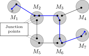
Figure 1. Construction of supergraphs described Section 4.2. The blue line represents the shortest path between $x$ and $y$.

1. Blobs: A collection $\{(M_{i},\mathrm{d}_{i},\mu_{i})\}_{i\in[m]}$ of connected, compact measured metric spaces.

2. Superstructure: A (random) graph $\mathcal{G}$ with vertex set $[m]$. The graph has a weight sequence $\mathbf{p}=(p_{i})_{i\in[m]}$ associated to the vertex set $[m]$. We regard $M_{i}$ as the $i$-th vertex of $\mathcal{G}$.

3. Junction points: An independent collection of random points $\mathbf{X}:=(X_{i,j}:i,j\in[m])$ such that $X_{i,j}\sim\mu_{i}$ for all $i,j$. Further, $\mathbf{X}$ is independent of $\mathcal{G}$.

Using these three ingredients, define a metric space $(\bar{M},\bar{\mathrm{d}},\bar{\mu})=\Gamma(\mathcal{G},\mathbf{p},\mathbf{M},\mathbf{X})$, with $\bar{M}=\sqcup_{i\in[m]}M_{i}$ (the disjoint union of the $M_{i}$’s) by putting an edge of length one between the pair of points $\{(X_{i,j},X_{j,i}):(i,j)\text{ is an edge of }\mathcal{G}\}.$ The distance metric $\bar{\mathrm{d}}$ is the natural metric obtained from the graph distance and the inter-blob distance on a path. More precisely, for any $x,y\in\bar{M}$ with $x\in M_{j_{1}}$ and $y\in M_{j_{2}}$,

$$\bar{\mathrm{d}}(x,y)=\inf\Big{\{}k+\mathrm{d}_{j_{1}}(x,X_{j_{1},i_{1}})+\sum_{l=1}^{k-1}\mathrm{d}_{i_{l}}(X_{i_{l},i_{l-1}},X_{i_{l},i_{l+1}})+\mathrm{d}_{j_{2}}(X_{j_{2},i_{k-1}},y)\Big{\}},$$ (4.2)

where the infimum is taken over all paths $(i_{1},\dots,i_{k-1})$ in $\mathcal{G}$ and all $k\geq 1$, and $i_{0}=j_{1}$ and $i_{k}=j_{2}$. The measure $\bar{\mu}$ is given by $\bar{\mu}(A):=\sum_{i\in[m]}p_{i}\mu_{i}(A\cap M_{i})$, for any measurable subset $A$ of $\bar{M}$. Note that there is a one-to-one correspondence between the components of $\mathcal{G}$ and $\Gamma(\mathcal{G},\mathbf{p},\mathbf{M},\mathbf{X})$ as the blobs are connected.

4.3. Space of trees with edge lengths, leaf weights, root-to-leaf measures, and blobs

In the proof of the main results we need the following spaces built on top of the space of discrete trees. The first space $T_{\scriptscriptstyle IJ}$ was formulated in [AP99, AP00a] where it was used to study trees spanning a finite number of random points sampled from an inhomogeneous continuum random tree (as described in the next section).

4.3.1. The space $T_{\scriptscriptstyle IJ}$

Fix $I\geq 0$ and $J\geq 1$. Let $T_{\scriptscriptstyle IJ}$ be the space of trees with each element $\mathbf{t}\in T_{\scriptscriptstyle IJ}$ having the following properties:

1. There are exactly $J$ leaves labeled $1+,\ldots,J+$, and the tree is rooted at the labeled vertex $0+$.

2. There may be extra labeled vertices (called hubs) with labels in $\left\{1,\ldots,I\right\}$. (It is possible that only some, and not all, labels in $\left\{1,\ldots,I\right\}$ are used.)

3. Every edge $e$ has a strictly positive edge length $l_{e}$.

A tree $\mathbf{t}\in T_{\scriptscriptstyle IJ}$ can be viewed as being composed of two parts: (1) $\operatorname{shape}(\mathbf{t})$ describing the shape of the tree (including the labels of leaves and hubs) but ignoring edge lengths. The set of all possible shapes $T_{\scriptscriptstyle IJ}^{\scriptscriptstyle\operatorname{shape}}$ is obviously finite for fixed $I,J$. (2) The edge lengths $\mathbf{l}(\mathbf{t}):=(l_{e}:e\in\mathbf{t})$. We will consider the product topology on $T_{\scriptscriptstyle IJ}$ consisting of the discrete topology on $T_{\scriptscriptstyle IJ}^{\scriptscriptstyle\operatorname{shape}}$ and the product topology on $\mathbb{R}^{\scriptscriptstyle\mathrm{E}(\mathbf{t})}$, where $\mathrm{E}(\mathbf{t})$ is the number of edges of $\mathbf{t}$.

4.3.2. The space $T_{\scriptscriptstyle IJ}^{*}$

Along with the three attributes above in $T_{\scriptscriptstyle IJ}$, the trees in $T_{\scriptscriptstyle IJ}^{*}$ have two additional properties. Let $\mathcal{L}(\mathbf{t}):=\left\{1+,\ldots,J+\right\}$ denote the collection of leaves in $\mathbf{t}$. Then every leaf $v\in\mathcal{L}(\mathbf{t})$ has the following attributes:

1. Leaf weights: A strictly positive number $A(v)$.

2. Root-to-leaf measures: A probability measure $\nu_{\mathbf{t},v}$ on the path $[0+,v]$ connecting the root and the leaf $v$.

For each $v\in\mathcal{L}(\mathbf{t})$, the path $[0+,v]$ can be viewed as a compact measured metric space with the measure being $\nu_{\mathbf{t},v}$. Let $\mathcal{X}$ denote the space of compact measured metric spaces endowed with the Gromov-Hausdorff-Prokhorov topology (see [BHS15, Section 2.1.1]). In addition to the topology on $T_{\scriptscriptstyle IJ}$, the space $T_{\scriptscriptstyle IJ}^{*}$ with the additional two attributes inherits the product topology on $\mathbb{R}^{\scriptscriptstyle J}$ due to leaf weights and $\mathcal{X}^{\scriptscriptstyle J}$ due to the paths $[0+,v]$ endowed with $\nu_{\mathbf{t},v}$ for each $v\in\mathcal{L}(\mathbf{t})$. For consistency, we add a conventional state $\partial$ to the spaces $T_{\scriptscriptstyle IJ}$ and $T_{\scriptscriptstyle IJ}^{*}$. Its use will be made clear in Section 5.

For all instances in this paper, the shape of a tree $\mathrm{shape}(\mathbf{t})$ will be viewed as a subgraph of a graph with $m$ vertices. In that case, the tree will be assumed to inherit the vertex labels from the original graph. We will often write $\mathbf{t}\in T^{*m}_{\scriptscriptstyle IJ}$ to emphasize the fact that the vertices of $\mathbf{t}$ are labeled from a subset of $[m]$.

4.3.3. The space $\overline{T}^{*m}_{\scriptscriptstyle IJ}$

We enrich the space $T^{*m}_{\scriptscriptstyle IJ}$ with some additional elements to accommodate the blobs. Consider $\mathbf{t}\in T_{\scriptscriptstyle IJ}^{*m}$ and construct $\bar{\mathbf{t}}$ as follows: Let $(M_{i},\mathrm{d}_{i},\mu_{i})_{i\in[m]}$ be a collection of blobs and $\mathbf{X}=(X_{ij}:i,j\in[m])$ be the collection of junction points as defined in Section 4.2. Construct the metric space $\bar{\mathbf{t}}$ with elements in $\bar{M}(\mathbf{t})=\sqcup_{i\in\mathbf{t}}M_{i}$, by putting an edge of length one between the pair of vertices $\{(X_{i,j},X_{j,i}):(i,j)\text{ is an edge of }\mathbf{t}\}.$ The distance metric is given by (4.2). The path from the leaf $v$ to the root $0+$ now contains blobs. Replace the root-to-leaf measure by $\bar{\nu}_{\mathbf{t},v}(A):=\sum_{i\in[0+,v]}\nu_{\mathbf{t},v}(i)\mu_{i}(M_{i}\cap A)$ for $A\subset\sqcup_{i\in[0+,v]}M_{i}$, where $\nu_{\mathbf{t},v}$ is the root-to-leaf measure on $[0+,v]$ for $\mathbf{t}$. Notice that $T_{\scriptscriptstyle IJ}^{*m}$ can be viewed as a subset of $\overline{T}_{\scriptscriptstyle IJ}^{*m}$. In the proof of the universality theorem in Section 5, the blobs will be a fixed collection and, therefore, any $\mathbf{t}\in T_{\scriptscriptstyle IJ}^{*m}$ corresponds to a unique $\bar{\mathbf{t}}\in\overline{T}_{\scriptscriptstyle IJ}^{*m}$.

4.4. $\mathbf{p}$-trees

For fixed $m\geq 1$, write $\mathbb{T}_{m}$ and $\mathbb{T}_{m}^{\scriptscriptstyle\operatorname{ord}}$ for the collection of all rooted trees with vertex set $[m]$ and rooted ordered trees with vertex set $[m]$ respectively. An ordered rooted tree is a rooted tree where children of each individual are assigned an order. We define a random tree model called $\mathbf{p}$-trees [CP99, P01], and their corresponding limits, the so-called inhomogeneous continuum random trees, which play a key role in describing the limiting metric spaces. Fix $m\geq 1$, and a probability mass function $\mathbf{p}=(p_{i})_{i\in[m]}$ with $p_{i}>0$ for all $i\in[m]$. A $\mathbf{p}$-tree is a random tree in $\mathbb{T}_{m}$, with law as follows: For any fixed $\mathbf{t}\in\mathbb{T}_{m}$ and $v\in\mathbf{t}$, write $d_{v}(\mathbf{t})$ for the number of children of $v$ in the tree $\mathbf{t}$. Then the law of the $\mathbf{p}$-tree, denoted by $\operatorname{\mathbbm{P}}_{\text{tree}}$, is defined as

$$\operatorname{\mathbbm{P}}_{\text{tree}}(\mathbf{t})=\operatorname{\mathbbm{P}}_{\text{tree}}(\mathbf{t};\mathbf{p})=\prod_{v\in[m]}p_{v}^{d_{v}(\mathbf{t})},\quad\mathbf{t}\in\mathbb{T}_{m}.$$ (4.3)

Note that a normalizing constant is not required in (4.3) to make it a probability distribution (see [CP99, Lemma 1]). Generating a random $\mathbf{p}$-tree $\mathscr{T}\sim\operatorname{\mathbbm{P}}_{\text{tree}}$ and then assigning a uniform random order on the children of every vertex $v\in\mathscr{T}$ gives a random element with law $\operatorname{\mathbbm{P}}_{\operatorname{ord}}(\cdot;\mathbf{p})$ given by

$$\operatorname{\mathbbm{P}}_{\operatorname{ord}}(\mathbf{t})=\operatorname{\mathbbm{P}}_{\operatorname{ord}}(\mathbf{t};\mathbf{p})=\prod_{v\in[m]}\frac{p_{v}^{d_{v}(\mathbf{t})}}{(d_{v}(\mathbf{t}))!},\quad\mathbf{t}\in\mathbb{T}_{m}^{\operatorname{ord}}.$$ (4.4)

4.4.1. The birthday construction of $\mathbf{p}$-trees

We now describe a construction of $\mathbf{p}$-trees, formulated in [CP99], that is relevant to this work. Let $\mathbf{Y}:=(Y_{0},Y_{1},\ldots)$ be a sequence of i.i.d. random variables with distribution $\mathbf{p}$. Let $R_{0}=0$ and for $l\geq 1$, let $R_{l}$ denote the $l$-th repeat time, i.e., $R_{l}=\min\big{\{}k>R_{l-1}:Y_{k}\in\{Y_{0},\ldots,Y_{k-1}\}\big{\}}.$ Now consider the directed graph formed via the edges $\mathcal{T}(\mathbf{Y}):=\left\{(Y_{j-1},Y_{j}):Y_{j}\notin\left\{Y_{0},\ldots,Y_{j-1}\right\},j\geq 1\right\}.$ This gives a tree which we view as rooted at $Y_{0}$. The following striking result was shown in [CP99]:

Theorem 4.1 ([CP99, Lemma 1 and Theorem 2]).

The random tree $\mathcal{T}(\mathbf{Y})$, viewed as an element in $\mathbb{T}_{m}$, is distributed as a $\mathbf{p}$-tree with distribution (4.3) independently of $Y_{R_{1}-1},Y_{R_{2}-1},\ldots$ which are i.i.d. with distribution $\mathbf{p}$.

Remark 8.

The independence between the sequence $Y_{R_{1}-1},Y_{R_{2}-1},\ldots$ and the constructed $\mathbf{p}$-tree $\mathcal{T}(\mathbf{Y})$ is truly remarkable. In particular, let $\mathcal{T}_{r}\subset\mathcal{T}(\mathbf{Y})$ denote the subtree with vertex set $\left\{Y_{0},Y_{1},\ldots,Y_{R_{r}-1}\right\}$, i.e., the tree constructed in the first $R_{r}$ steps. Further take $\tilde{\mathbf{Y}}=(\tilde{Y_{1}},\ldots,\tilde{Y_{r}})$ to be an i.i.d. sample from $\mathbf{p}$ and then construct the subtree $\mathcal{S}_{r}$ spanned by $\tilde{\mathbf{Y}}$. Then the above result (formalized as [CP99, Corollary 3]) implies that

$$(\tilde{Y_{1}},\tilde{Y_{2}},\ldots,\tilde{Y_{r}};\mathcal{S}_{r})\stackrel{{\scriptstyle d}}{{=}}(Y_{R_{1}-1},Y_{R_{2}-1},\ldots,Y_{R_{r}-1};\mathcal{T}_{r}).$$ (4.5)

We will use this fact in Section 5 to complete the proof of the universality theorem.

4.4.2. Tilted $\mathbf{p}$-trees and connected components of $\mathrm{NR}_{n}(\boldsymbol{x},t)$

Consider the vertex set $[n]$ and assign weight $x_{i}$ to vertex $i$. Now, connect each pair of vertices $i,j$ ($i\neq j$) independently with probability $q_{ij}:=1-\exp(-tx_{i}x_{j}).$ The resulting random graph, denoted by $\mathrm{NR}_{n}(\boldsymbol{x},t)$, is known as the Norros-Reittu model or the Poisson graph process [RGCN1]. For a connected component $\mathcal{C}\subseteq\mathrm{NR}_{n}(\boldsymbol{x},t)$, let $\operatorname{mass}(\mathcal{C}):=\sum_{i\in\mathcal{C}}x_{i}$ and, for any $t\geq 0$, let $(\mathcal{C}_{i}(t))_{i\geq 1}$ denote the components in decreasing order of their mass sizes. In this section, we describe results from [BSW14] that give a method of constructing connected components of $\mathrm{NR}_{n}(\boldsymbol{x},t)$, conditionally on the vertices of the components. This construction involves tilted versions of $\mathbf{p}$-trees introduced in Section 4.4. Since these trees are parametrized via a driving probability mass function (pmf) $\mathbf{p}$, it will be easy to parametrize various random graph constructions in terms of pmfs as opposed to the vertex weights $\boldsymbol{x}$. Proposition 4.2 will relate vertex weights to pmfs.

Fix $n\geq 1$ and $\mathcal{V}\subset[n]$, and write $\mathbb{G}_{\mathcal{V}}^{\operatorname{con}}$ for the space of all simple connected graphs with vertex set $\mathcal{V}$. For fixed $a>0$, and probability mass function $\mathbf{p}=(p_{v})_{v\in\mathcal{V}}$, define probability distributions $\operatorname{\mathbbm{P}}_{\operatorname{con}}(\cdot;\mathbf{p},a,\mathcal{V})$ on $\mathbb{G}_{\mathcal{V}}^{\operatorname{con}}$ as follows: For $i,j\in\mathcal{V}$, denote

$$q_{ij}:=1-\exp(-ap_{i}p_{j}).$$ (4.6)

Then, for $G\in\mathbb{G}_{\mathcal{V}}^{\operatorname{con}},$

$$\operatorname{\mathbbm{P}}_{\operatorname{con}}(G;\mathbf{p},a,\mathcal{V}):=\frac{1}{Z(\mathbf{p},a)}\prod_{(i,j)\in E(G)}q_{ij}\prod_{(i,j)\notin E(G)}(1-q_{ij}),$$ (4.7)

where $Z(\mathbf{p},a)$ is the normalizing constant. Now let $\mathcal{V}^{\scriptscriptstyle(i)}$ be the vertex set of $\mathcal{C}_{i}(t)$ for $i\geq 1$, and note that $(\mathcal{V}^{\scriptscriptstyle(i)})_{i\geq 1}$ denotes a random finite partition of the vertex set $[n]$. The next proposition yields a construction of the random (connected) graphs $(\mathcal{C}_{i}(t))_{i\geq 1}$:

Proposition 4.2 ([BSW14, Proposition 6.1]).

Given the partition $(\mathcal{V}^{\scriptscriptstyle(i)})_{i\geq 1}$, define, for $i\geq 1$,

$$\mathbf{p}_{n}^{\scriptscriptstyle(i)}:=\left(\frac{x_{v}}{\sum_{v\in\mathcal{V}^{\scriptscriptstyle(i)}}x_{v}}:v\in\mathcal{V}^{\scriptscriptstyle(i)}\right),\quad a_{n}^{\scriptscriptstyle(i)}:=t\bigg{(}\sum_{v\in\mathcal{V}_{\scriptscriptstyle(i)}}x_{v}\bigg{)}^{2}.$$ (4.8)

For each fixed $i\geq 1$, let $G_{i}\in\mathbb{G}_{\mathcal{V}^{\scriptscriptstyle(i)}}^{\operatorname{con}}$ be a connected simple graph with vertex set $\mathcal{V}^{\scriptscriptstyle(i)}$. Then

$$\operatorname{\mathbbm{P}}\left(\mathcal{C}_{i}(t)=G_{i},\;\;\forall i\geq 1\ \big{|}\ (\mathcal{V}^{\scriptscriptstyle(i)})_{i\geq 1}\right)=\prod_{i\geq 1}\operatorname{\mathbbm{P}}_{\operatorname{con}}(G_{i};\mathbf{p}_{n}^{\scriptscriptstyle(i)},a_{n}^{\scriptscriptstyle(i)},\mathcal{V}^{\scriptscriptstyle(i)}).$$ (4.9)

Proposition 4.2 yields the following construction of $\mathrm{NR}_{n}(\boldsymbol{x},t)$:

Algorithm 1.

The random graph $\mathrm{NR}_{n}(\boldsymbol{x},t)$ can be generated in two stages:

1. Generate the random partition $(\mathcal{V}^{\scriptscriptstyle(i)})_{i\geq 1}$ of the vertices into different components.

2. Conditionally on the partition, generate the internal structure of each component following the law of $\operatorname{\mathbbm{P}}_{\operatorname{con}}(\cdot;\mathbf{p}^{\scriptscriptstyle(i)},a^{\scriptscriptstyle(i)},\mathcal{V}^{\scriptscriptstyle(i)})$, independently across different components.

Let us now describe an algorithm to generate such connected components using distribution (4.7). To ease notation, let $\mathcal{V}=[m]$ for some $m\geq 1$ and fix a probability mass function $\mathbf{p}$ on $[m]$ and a constant $a>0$ and write $\operatorname{\mathbbm{P}}_{\operatorname{con}}(\cdot):=\operatorname{\mathbbm{P}}_{\operatorname{con}}(\cdot;\mathbf{p},a,[m])$ on $\mathbb{G}_{m}^{\operatorname{con}}:=\mathbb{G}_{[m]}^{\operatorname{con}}$. To generate a sample $G$ from $\operatorname{\mathbbm{P}}_{\operatorname{con}}$, one needs to first generate a $\mathbf{p}$-tree (with suitable tilt). The rest of the edges of $G$ are surplus edges, which are generated by connecting the leaves to one of the vertices in their path to the root. Let us now describe this process formally. As a matter of convention, we view ordered rooted trees via their planar embedding using the associated ordering to determine the relative locations of siblings of an individual. We think of the left most sibling as the "oldest". Further, in a depth-first exploration, we explore the tree from left to right. Now given a planar rooted tree $\mathbf{t}\in\mathbb{T}_{m}$, let $\rho$ denote the root, and for every vertex $v\in[m]$, let $[\rho,v]$ denote the path connecting $\rho$ to $v$ in the tree. Given this path and a vertex $i\in[\rho,v]$, write $\mathrm{RC}(i,[\rho,v])$ for the set of all children of $i$ that fall to the right of $[\rho,v]$. Define $\mathfrak{P}(v,\mathbf{t}):=\cup_{i\in[m]}\mathrm{RC}(i,[\rho,v]).$ In the terminology of [ABG09, BHS15], $\mathfrak{P}(v,\mathbf{t})$ denotes the set of endpoints of all permitted edges emanating from $v$. Define

$$\mathfrak{G}_{\scriptscriptstyle(m)}(v):=\sum_{i\in[\rho,v]}\sum_{j\in[m]}p_{j}\mathbbm{1}\left\{j\in\mathrm{RC}(i,[\rho,v])\right\}.$$ (4.10)

Let $(v(1),v(2),\ldots,v(m))$ denote the order of the vertices in the depth-first exploration of the tree $\mathbf{t}$. Let $y^{*}(0)=0$ and $y^{*}(i)=y^{*}(i-1)+p_{v(i)}$ and define

$$A_{\scriptscriptstyle(m)}(u)=\mathfrak{G}_{\scriptscriptstyle(m)}(v(i)),\ \text{ for }u\in(y^{*}(i-1),y^{*}(i)],\quad\text{and}\quad\bar{A}_{\scriptscriptstyle(m)}(\cdot):=aA_{\scriptscriptstyle(m)}(\cdot),$$ (4.11)

where $a$ is defined in (4.6). Define the function

$$\Lambda_{\scriptscriptstyle(m)}(\mathbf{t}):=a\sum_{v\in[m]}p_{v}\mathfrak{G}_{\scriptscriptstyle(m)}(v).$$ (4.12)

Finally, let $\mathrm{E}(\mathbf{t})$ denote the set of edges of $\mathbf{t}$, $\mathscr{T}_{m}^{\mathbf{p}}$ the $\mathbf{p}$-tree defined in (4.4), $\mathfrak{P}(\mathbf{t})=\cup_{v\in[m]}\mathfrak{P}(v,\mathbf{t})$, and define the function $L:\mathbb{T}_{m}^{\operatorname{ord}}\to\mathbb{R}_{+}$ by

$$L(\mathbf{t})=\displaystyle L_{\scriptscriptstyle(m)}(\mathbf{t}):=\prod_{(k,\ell)\in\mathrm{E}(\mathbf{t})}\left[\frac{\exp(ap_{k}p_{\ell})-1}{ap_{k}p_{\ell}}\right]\exp\bigg{(}\sum_{(k,\ell)\in\mathfrak{P}(\mathbf{t})}ap_{k}p_{\ell}\bigg{)},$$ (4.13)

for $\mathbf{t}\in\mathbb{T}_{m}^{\operatorname{ord}}$. Recall the (ordered) $\mathbf{p}$-tree distribution from (4.4). Let $\mathscr{T}^{\mathbf{p}}_{m}$ be a sample from $\operatorname{\mathbbm{P}}_{\operatorname{ord}}$. Using $L(\cdot)$ to tilt this distribution results in the distribution

$$\operatorname{\mathbbm{P}}_{\operatorname{ord}}^{\star}(\mathbf{t}):=\operatorname{\mathbbm{P}}_{\operatorname{ord}}(\mathbf{t})\cdot\frac{L(\mathbf{t})}{\mathbbm{E}_{\operatorname{ord}}[L(\mathscr{T}^{\mathbf{p}}_{m})]},\qquad\mathbf{t}\in\mathbb{T}_{m}^{\operatorname{ord}}.$$ (4.14)

In the algorithm below, all the objects depend on the tree $\mathbf{t}$, but we often suppress this dependence to ease notation.

Algorithm 2.

Let $\tilde{\mathcal{G}}_{m}(\mathbf{p},a)$ denote a random graph sampled from $\mathbbm{P}_{\mathrm{con}}(\cdot)$. This algorithm gives a construction of $\tilde{\mathcal{G}}_{m}(\mathbf{p},a)$, proved in [BHS15]:

1. Tilted $\mathbf{p}$-tree: Generate a tilted ordered $\mathbf{p}$-tree $\mathscr{T}^{\mathbf{p},\star}_{m}$ with distribution (4.14). Now consider the (random) objects $\mathfrak{P}(v,\mathscr{T}^{\mathbf{p},\star}_{m})$ for $v\in[m]$ and the corresponding (random) functions $\mathfrak{G}_{\scriptscriptstyle(m)}(\cdot)$ on $[m]$ and $A_{\scriptscriptstyle(m)}(\cdot)$ on $[0,1]$.

2. Poisson number of possible surplus edges: Let $\mathcal{P}$ denote a rate-one Poisson process on $\mathbb{R}_{+}^{2}$ and define

   $$\bar{A}_{\scriptscriptstyle(m)}\cap{\mathcal{P}}:=\left\{(s,t)\in\mathcal{P}:s\in[0,1],t\leq\bar{A}_{\scriptscriptstyle(m)}(s)\right\}.$$ (4.15)

   Write $\bar{A}_{\scriptscriptstyle(m)}\cap{\mathcal{P}}:=\{(s_{j},t_{j}):1\leq j\leq N_{\scriptscriptstyle(m)}^{\star}\}$ where $N_{\scriptscriptstyle(m)}^{\star}=|\bar{A}_{\scriptscriptstyle(m)}\cap{\mathcal{P}}|$. We next use the set $\{(s_{j},t_{j}):1\leq j\leq N_{\scriptscriptstyle(m)}^{\star}\}$ to generate pairs of points $\left\{(\mathcal{L}_{j},\mathcal{R}_{j}):1\leq j\leq N_{\scriptscriptstyle(m)}^{\star}\right\}$ in the tree that will be joined to form the surplus edges.

3. First endpoints: Fix $j$ and suppose $s_{j}\in(y^{*}(i-1),y^{*}(i)]$ for some $i\geq 1$, where $y^{*}(i)$ is as given right above (4.11). Then the first endpoint of the surplus edge corresponding to $(s_{j},t_{j})$ is $\mathcal{L}_{j}:=v(i)$.

4. Second endpoints: Note that in the interval $(y^{*}(i-1),y^{*}(i)]$, the function $\bar{A}_{\scriptscriptstyle(m)}$ is of constant value $a\mathfrak{G}_{\scriptscriptstyle(m)}(v(i))$. We will view this value or height as being partitioned into sub-intervals of length $ap_{u}$ for each $u\in\mathfrak{P}(v(i),\mathscr{T}^{\mathbf{p},\star}_{m})$, the collection of endpoints of permitted edges emanating from $\mathcal{L}_{k}$. (Assume that this partitioning is done according to some preassigned rule, e.g., using the order of the vertices in $\mathfrak{P}(v(i),\mathscr{T}^{\mathbf{p},\star}_{m})$). Suppose that $t_{j}$ belongs to the interval corresponding to $u$. Then the second endpoint is $\mathcal{R}_{j}=u$. Form an edge between $(\mathcal{L}_{j},\mathcal{R}_{j})$.

5. In this construction, it is possible that one creates more than one surplus edge between two vertices. Remove any multiple surplus edges. This has vanishing probability in our applications.

Definition 1.

Consider the connected random graph $\tilde{\mathcal{G}}_{m}(\mathbf{p},a)$, given by Algorithm 2, viewed as a measured metric space via the graph distance and each vertex $v$ is assigned measure $p_{v}$.

Lemma 4.1 ([BHS15, Lemma 4.10]).

The random graph $\tilde{\mathcal{G}}_{m}(\mathbf{p},a)$ generated by Algorithm 2 has the same law as $\mathbbm{P}_{\mathrm{con}}(\cdot)$. Further, conditionally on $\mathscr{T}^{\mathbf{p},\star}_{m}$, the following hold:

1. $N_{\scriptscriptstyle(m)}^{\star}$ has Poisson distribution with mean $\Lambda_{\scriptscriptstyle(m)}(\mathscr{T}_{m}^{\mathbf{p},\star})$, where $\Lambda_{\scriptscriptstyle(m)}$ is as in (4.12).

2. Conditionally on $\mathscr{T}_{m}^{\mathbf{p},\star}$ and $N_{\scriptscriptstyle(m)}^{\star}=k$, the first endpoints $(\mathcal{L}_{j})_{j\in[k]}$ can be generated in an i.i.d. fashion by sampling from the vertex set $[m]$ with probability distribution $\mathcal{J}^{\scriptscriptstyle(m)}(v)\propto p_{v}\mathfrak{G}_{\scriptscriptstyle(m)}(v),$ $v\in[m].$

3. Conditionally on $\mathscr{T}_{m}^{\mathbf{p},\star}$, $N_{\scriptscriptstyle(m)}^{\star}=k$ and the first endpoints $(\mathcal{L}_{j})_{j\in[k]}$, generate the second endpoints in an i.i.d. fashion where conditionally on $\mathcal{L}_{j}=v$, the probability distribution of $\mathcal{R}_{j}$ is given by

   $$Q_{v}^{\scriptscriptstyle(m)}(y):=\begin{cases}\sum_{u}p_{u}\mathbbm{1}\left\{u\in\mathrm{RC}(y,[\rho,v])\right\}/\mathfrak{G}_{\scriptscriptstyle(m)}(v)&\text{ if }y\in[\rho,v],\\ 0&\text{ otherwise}.\end{cases}$$ (4.16)

   Create an edge between $\mathcal{L}_{j}$ and $\mathcal{R}_{j}$ for $1\leq j\leq k$.

4.5. Inhomogeneous continuum random trees

In a series of papers [AMP04, AP99, AP00a] it was shown that $\mathbf{p}$-trees, under various assumptions, converge to inhomogeneous continuum random trees (ICRTs) that we now describe. Recall from [E06, LG05] that a real tree is a metric space $(\mathscr{T},d)$ that satisfies the following for every pair $a,b\in\mathscr{T}$:

1. There is a unique isometric map $f_{a,b}\colon[0,d(a,b)]\to\mathscr{T}$ such that $f_{a,b}(0)=a$ and $f_{a,b}(d(a,b))=b$.

2. For any continuous one-to-one map $g:[0,1]\to\mathscr{T}$ with $g(0)=a$ and $g(1)=b$, we have $g([0,1])=f_{a,b}([0,d(a,b)])$.

Construction of the ICRT: Given $\boldsymbol{\beta}\in\ell^{2}_{{\scriptscriptstyle\downarrow}}\setminus\ell^{1}_{{\scriptscriptstyle\downarrow}}$ with $\sum_{i}\beta_{i}^{2}=1$, we will now define the inhomogeneous continuum random tree $\mathscr{T}^{\boldsymbol{\beta}}$. We mainly follow the notation in [AP00a]. Assume that we are working on a probability space $(\Omega,\mathcal{F},\operatorname{\mathbbm{P}}_{\boldsymbol{\beta}})$ rich enough to support the following:

1. For each $i\geq 1$, let $\mathcal{P}_{i}:=(\xi_{i,1},\xi_{i,2},\ldots)$ be rate $\beta_{i}$ Poisson processes that are independent for different $i$. The first point of each process $\xi_{i,1}$ is special and is called a joinpoint, while the remaining points $\xi_{i,j}$ with $j\geq 2$ will be called $i$-cutpoints [AP00a].

2. Independently of the above, let $\boldsymbol{U}=(U_{j}^{\scriptscriptstyle(i)})_{i,j\geq 1}$ be a collection of i.i.d uniform $(0,1)$ random variables. These are not required to construct the tree but will be used to define a certain function on the tree.

The random real tree (with marked vertices) $\mathscr{T}_{\scriptscriptstyle(\infty)}^{\boldsymbol{\beta}}$ is then constructed as follows:

1. Arrange the cutpoints $\left\{\xi_{i,j}:i\geq 1,j\geq 2\right\}$ in increasing order as $0<\eta_{1}<\eta_{2}<\cdots$. The assumption that $\sum_{i}\beta_{i}^{2}<\infty$ implies that this is possible. For every cutpoint $\eta_{k}=\xi_{i,j}$, let $\eta_{k}^{*}:=\xi_{i,1}$ be the corresponding joinpoint.

2. Next, build the tree inductively. Start with the branch $[0,\eta_{1}]$. Inductively assuming that we have completed step $k$, attach the branch $(\eta_{k},\eta_{k+1}]$ to the joinpoint $\eta_{k}^{*}$ corresponding to $\eta_{k}$.

Write $\mathscr{T}_{0}^{\boldsymbol{\beta}}$ for the corresponding tree after one has used up all the branches $[0,\eta_{1}]$, $\left\{(\eta_{k},\eta_{k+1}]:k\geq 1\right\}$. Note that for every $i\geq 1$, the joinpoint $\xi_{i,1}$ corresponds to a vertex with infinite degree. Label this vertex $i$. The ICRT $\mathscr{T}_{\scriptscriptstyle(\infty)}^{\boldsymbol{\beta}}$ is the completion of the marked metric tree $\mathscr{T}^{\boldsymbol{\beta}}_{0}$. As argued in [AP00a, Section 2], this is a real-tree as defined above which can be viewed as rooted at the vertex corresponding to zero. We call the vertex corresponding to joinpoint $\xi_{i,1}$ hub $i$.

Figure 2. An illustration of the ICRT construction with four point process $\left\{\mathcal{P}_{i}:1\leq i\leq 4\right\}$. The red points represent the joinpoint of the corresponding point process and the blue points the corresponding cutpoints. The last line contains the union of the four point processes. See Figure 3 for the corresponding tree.

Figure 3. The tree constructed via the stick-breaking construction from Figure 2.

The uniform random variables $(U_{j}^{\scriptscriptstyle(i)})_{i,j\geq 1}$ give rise to a natural ordering on $\mathscr{T}_{\scriptscriptstyle(\infty)}^{\boldsymbol{\beta}}$ (or a planar embedding of $\mathscr{T}_{\scriptscriptstyle(\infty)}^{\boldsymbol{\beta}}$) as follows: For $i\geq 1$, let $(\mathscr{T}_{j}^{\scriptscriptstyle(i)})_{j\geq 1}$ be the collection of subtrees hanging off the $i$-th hub. Associate $U_{j}^{\scriptscriptstyle(i)}$ with the subtree $\mathscr{T}_{j}^{\scriptscriptstyle(i)}$, and think of $\mathscr{T}_{j_{1}}^{\scriptscriptstyle(i)}$ appearing "to the right of" $\mathscr{T}_{j_{2}}^{\scriptscriptstyle(i)}$ if $U_{j_{1}}^{\scriptscriptstyle(i)}<U_{j_{2}}^{\scriptscriptstyle(i)}$. This is the natural ordering on $\mathscr{T}_{\scriptscriptstyle(\infty)}^{\boldsymbol{\beta}}$ when it is being viewed as a limit of ordered $\mathbf{p}$-trees. We can think of the pair $(\mathscr{T}_{\scriptscriptstyle(\infty)}^{\boldsymbol{\beta}},\boldsymbol{U})$ as the ordered ICRT.

4.6. Continuum limits of components

The aim of this section is to give an explicit description of the limiting (random) metric spaces in Theorem 2.1. We start by constructing a specific metric space using the tilted version of the ICRT in Section 4.6.1. Then we describe the limits of maximal components in Section 4.6.3.

4.6.1. Tilted ICRTs and vertex identification

Let $(\Omega,\mathcal{F},\operatorname{\mathbbm{P}}_{\beta})$ and $\mathscr{T}_{\scriptscriptstyle(\infty)}^{\boldsymbol{\beta}}$ be as in Section 4.5. In [AP00a], it was shown that one can associate a natural probability measure $\mu$, called the mass measure, to $\mathscr{T}_{\scriptscriptstyle(\infty)}^{\boldsymbol{\beta}}$, satisfying $\mu(\mathcal{L}(\mathscr{T}_{\scriptscriptstyle(\infty)}^{\boldsymbol{\beta}}))=1$. Here we recall that $\mathcal{L}(\cdot)$ denotes the set of leaves. Before moving to the desired construction of the random metric space, we will need to define some more quantities that describe the asymptotic analogues of the quantities appearing in Algorithm 2. Similarly to (4.10), define $\mathfrak{G}_{\scriptscriptstyle(\infty)}(y)=\sum_{i\geq 1}\beta_{i}\big{(}\sum_{j\geq 1}U_{j}^{\scriptscriptstyle(i)}\times\mathbbm{1}\{y\in\mathscr{T}_{j}^{\scriptscriptstyle(i)}\}\big{)}.$ It was shown in [BHS15] that $\mathfrak{G}_{\scriptscriptstyle(\infty)}(y)$ is finite for almost every realization of $\mathscr{T}_{\scriptscriptstyle(\infty)}^{\boldsymbol{\beta}}$ and for $\mu$-almost every $y\in\mathscr{T}_{\scriptscriptstyle(\infty)}^{\boldsymbol{\beta}}$. For $y\in\mathscr{T}_{\scriptscriptstyle(\infty)}^{\boldsymbol{\beta}}$, let $[\rho,y]$ denote the path from the root $\rho$ to $y$. For every $y$, define a probability measure on $[\rho,y]$ as

$$Q_{y}^{\scriptscriptstyle(\infty)}(v):=\frac{\beta_{i}U_{j}^{\scriptscriptstyle(i)}}{\mathfrak{G}_{\scriptscriptstyle(\infty)}(y)},\quad\mbox{ if }v\mbox{ is the }i\mbox{-th hub and }y\in\mathscr{T}_{j}^{\scriptscriptstyle(i)}\mbox{ for some }j.$$ (4.17)

Thus, this probability measure is concentrated on the hubs on the path from $y$ to the root. Let $\gamma>0$ be a constant. Informally, the construction goes as follows: We will first tilt the distribution of the original ICRT $\mathscr{T}_{\scriptscriptstyle(\infty)}^{\boldsymbol{\beta}}$ using the exponential functional

$$L_{\scriptscriptstyle(\infty)}(\mathscr{T}_{\scriptscriptstyle(\infty)}^{\boldsymbol{\beta}},\boldsymbol{U}):=\exp\bigg{(}\gamma\int_{y\in\mathscr{T}_{\scriptscriptstyle(\infty)}^{\boldsymbol{\beta}}}\mathfrak{G}_{\scriptscriptstyle(\infty)}(y)\mu(dy)\bigg{)}$$ (4.18)

to get a tilted tree $\mathscr{T}_{\scriptscriptstyle(\infty)}^{\boldsymbol{\beta},\star}$. We then generate a random but finite number $N_{\scriptscriptstyle(\infty)}^{\star}$ of pairs of points $\{(x_{k},y_{k}):1\leq k\leq N_{\scriptscriptstyle(\infty)}^{\star}\}$ that will provide the surplus edges. The final metric space is obtained by creating shortcuts by identifying the points $x_{k}$ and $y_{k}$. The construction mimics that of Algorithm 2. Formally the construction proceeds in four steps:

1. Tilted ICRT: Define ${\operatorname{\mathbbm{P}}}_{\beta}^{\star}$ on $\Omega$ by

   $$\frac{d{{\operatorname{\mathbbm{P}}}}_{\beta}^{\star}}{d{{\operatorname{\mathbbm{P}}}}_{\beta}}=\frac{\exp\big{(}\gamma\int_{y\in\mathscr{T}^{\boldsymbol{\beta}}_{(\infty)}}\mathfrak{G}_{(\infty)}(y)\mu(dy)\big{)}}{\mathbbm{E}\Big{[}\exp\big{(}\gamma\int_{x\in\mathscr{T}^{\boldsymbol{\beta}}_{(\infty)}}\mathfrak{G}_{\scriptscriptstyle(\infty)}(x)\mu(dx)\big{)}\Big{]}}.$$ (4.19)

   The expectation in the denominator is with respect to the original measure ${\operatorname{\mathbbm{P}}}_{\beta}$. Write $(\mathscr{T}_{\scriptscriptstyle(\infty)}^{\boldsymbol{\beta},\star},\mu^{\star})$ and $\boldsymbol{U}^{\star}=(U_{j}^{(i),\star})_{i,j\geq 1}$ for the tree and the mass measure on it, and the associated random variables under this change of measure.

2. Poisson number of identification points: Conditionally on $((\mathscr{T}_{\scriptscriptstyle(\infty)}^{\boldsymbol{\beta},\star},\mu^{\star}),\boldsymbol{U}^{\star})$, generate $N_{\scriptscriptstyle(\infty)}^{\star}$ having a $\mathrm{Poisson}(\Lambda_{\scriptscriptstyle(\infty)}^{\star})$ distribution, where

   $$\Lambda_{\scriptscriptstyle(\infty)}^{\star}:=\gamma\int_{y\in\mathscr{T}_{\scriptscriptstyle(\infty)}^{\boldsymbol{\beta},\star}}\mathfrak{G}_{\scriptscriptstyle(\infty)}(y)\mu^{\star}(dy)=\gamma\sum_{i\geq 1}\beta_{i}\bigg{[}\sum_{j\geq 1}U_{j}^{(i),\star}\mu^{\star}(\mathscr{T}_{j}^{\scriptscriptstyle(i),\star})\bigg{]}.$$ (4.20)

   Here, $(\mathscr{T}_{j}^{\scriptscriptstyle(i),\star})_{j\geq 1}$ denotes the collection of subtrees of hub $i$ in $\mathscr{T}_{\scriptscriptstyle(\infty)}^{\boldsymbol{\beta},\star}$.

3. First endpoints (of shortcuts): Conditionally on (a) and (b), sample $x_{k}$ from $\mathscr{T}_{\scriptscriptstyle(\infty)}^{\boldsymbol{\beta},\star}$ with density proportional to $\mathfrak{G}_{\scriptscriptstyle(\infty)}(x)\mu^{\star}(dx)$ for $1\leq k\leq N_{\scriptscriptstyle(\infty)}^{\star}$.

4. Second endpoints (of shortcuts) and identification: Having chosen $x_{k}$, choose $y_{k}$ from the path $[\rho,x_{k}]$ joining the root $\rho$ and $x_{k}$ according to the probability measure $Q_{x_{k}}^{\scriptscriptstyle(\infty)}$ as in (4.17) but with $U_{j}^{(i),\star}$ replacing $U_{j}^{\scriptscriptstyle(i)}$. (Note that $y_{k}$ is always a hub on $[\rho,x_{k}]$.) Identify $x_{k}$ and $y_{k}$, i.e., form the quotient space by introducing the equivalence relation $x_{k}\sim y_{k}$ for $1\leq k\leq N_{\scriptscriptstyle(\infty)}^{\star}$.

Definition 2.

Fix $\gamma\geq 0$ and $\boldsymbol{\beta}\in\ell^{2}_{{\scriptscriptstyle\downarrow}}\setminus\ell^{1}_{{\scriptscriptstyle\downarrow}}$ with $\sum_{i}\beta_{i}^{2}=1$. Let $\mathcal{G}_{\scriptscriptstyle(\infty)}(\boldsymbol{\beta},\gamma)$ be the metric measure space constructed via the four steps above equipped with the measure inherited from the mass measure on $\mathscr{T}_{\scriptscriptstyle(\infty)}^{\boldsymbol{\beta},\star}$.

4.6.2. Scaling limit for the component sizes and surplus edges

Let us describe the scaling limit results for the component sizes and the surplus edges ($\#\text{edges}-\#\text{vertices}+1$) for the largest components of $\mathrm{CM}_{n}(\boldsymbol{d},p_{n}(\lambda))$ from [DHLS16]. Although we need to define the limiting object only for describing the limiting metric space, the convergence result will turn out to be crucial in Section LABEL:sec:proof-metric-mc in the proof of Theorem 2.1, and therefore we state it here as well. Consider a decreasing sequence $\boldsymbol{\theta}\in\ell^{3}_{{\scriptscriptstyle\downarrow}}\setminus\ell^{2}_{{\scriptscriptstyle\downarrow}}$. Denote by $\mathcal{I}_{i}(s):=\mathbbm{1}\left\{\zeta_{i}\leq s\right\}$ where $\zeta_{i}\sim\mathrm{Exp}(\theta_{i})$ independently, and $\mathrm{Exp}(r)$ denotes the exponential distribution with rate $r$. Consider the process

$$\bar{S}^{\lambda}_{\infty}(t)=\sum_{i=1}^{\infty}\theta_{i}\left(\mathcal{I}_{i}(t)-\theta_{i}t\right)+\lambda t,$$ (4.21)

for some $\lambda\in\mathbbm{R}$. Define the reflected version of $\bar{S}_{\infty}^{\lambda}(t)$ by $\mathrm{refl}\big{(}\bar{S}_{\infty}^{\lambda}(t)\big{)}=\bar{S}_{\infty}^{\lambda}(t)-\inf_{0\leq u\leq t}\bar{S}_{\infty}^{\lambda}(u).$ The processes of the form (4.21) were termed thinned Lévy processes in [BHL12] since the summands are thinned versions of Poisson processes. Let $(\Xi_{i}(\boldsymbol{\theta},\lambda))_{i\geq 1}$, $(\xi_{i}(\boldsymbol{\theta},\lambda))_{i\geq 1}$, respectively, denote the vector of excursions and excursion-lengths of $\big{(}\mathrm{refl}(\bar{S}_{\infty}^{\lambda}(t))\big{)}_{t\geq 0}$, ordered according to the excursion lengths in a decreasing manner. Using [DHLS16, Fact 1], there are no ties among the excursion lengths almost surely. Denote the vector $(\xi_{i}(\boldsymbol{\theta},\lambda))_{i\geq 1}$ by $\boldsymbol{\xi}(\boldsymbol{\theta},\lambda)$. The fact that $\boldsymbol{\xi}(\boldsymbol{\theta},\lambda)$ is always well defined follows from [AL98, Lemma 1]. Also, define the counting process of marks $\mathbf{N}$ to be a Poisson process that has intensity $\mathrm{refl}\left(\bar{S}_{\infty}^{\lambda}(t)\right)$ at time $t$ conditional on $(\mathrm{refl}\left(\bar{S}_{\infty}^{\lambda}(u)\right))_{u\leq t}$. We use the notation $\mathscr{N}_{i}(\boldsymbol{\theta},\lambda)$ to denote the number of marks within $\Xi_{i}(\boldsymbol{\theta},\lambda)$.

For a connected graph $G$, let $\mathrm{SP}(G)=\#\text{edges}-\#\text{vertices}+1$ denote its surplus edges. In the context of this paper, we simply write $\xi_{i}$, $\boldsymbol{\xi}$ and $\mathscr{N}_{i}$ respectively for $\xi_{i}(\boldsymbol{\theta}/(\mu\nu),\lambda/\mu)$, $\boldsymbol{\xi}(\boldsymbol{\theta}/(\mu\nu),\lambda/\mu)$ and $\mathscr{N}_{i}(\boldsymbol{\theta}/(\mu\nu),\lambda/\mu)$.

Proposition 4.3 ([DHLS16, Theorem 4]).

Under Assumption 1, as $n\to\infty$,

$$\big{(}n^{-\rho}|\mathscr{C}_{\scriptscriptstyle(i)}^{p}(\lambda)|,\mathrm{SP}(\mathscr{C}_{\scriptscriptstyle(i)}^{p}(\lambda))\big{)}_{i\geq 1}\xrightarrow{d}\Big{(}\frac{1}{\nu}\xi_{i},\mathscr{N}_{i}\Big{)}_{i\geq 1},$$ (4.22)

with respect to the topology on the product space $\ell^{2}_{\scriptscriptstyle\downarrow}\times\mathbb{N}^{\mathbb{N}}$.

The limiting object in [DHLS16, Theorem 4] is stated in a slightly different form compared to the right hand side of (4.22). However, the limiting objects are identical in distribution with suitable rescaling of time and space, and by observing that $r\mathrm{Exp}(r)\stackrel{{\scriptstyle\scriptscriptstyle d}}{{=}}\mathrm{Exp}(1)$, where $\mathrm{Exp}(r)$ denotes an exponential random variable with rate $r$ (see Appendix LABEL:sec:appendix-rescaling). In fact, the arguments in Appendix LABEL:sec:appendix-rescaling establish the following lemma which will be used extensively in Section LABEL:sec:proof-metric-mc:

Lemma 4.2.

For $\eta_{1},\eta_{2}>0$, $\boldsymbol{\theta}\in\ell^{3}_{{\scriptscriptstyle\downarrow}}\setminus\ell^{2}_{{\scriptscriptstyle\downarrow}}$ and $\lambda\in\mathbb{R}$, $\boldsymbol{\xi}(\eta_{1}\boldsymbol{\theta},\eta_{2}\lambda)\stackrel{{\scriptstyle d}}{{=}}\frac{1}{\eta_{1}}\boldsymbol{\xi}\big{(}\boldsymbol{\theta},\frac{\eta_{2}}{\eta_{1}^{2}}\lambda\big{)}.$

4.6.3. Limiting component structures

We are now all set to describe the metric space $M_{i}$ appearing in Theorem 2.1. Recall the graph $\mathcal{G}_{\infty}(\boldsymbol{\beta},\gamma)$ from Definition 2. Using the notation of Section 4.6.2, write $\xi_{i}^{*}$ for $\xi_{i}((\mu(\nu-1))^{-1}\boldsymbol{\theta},(\mu(\nu-1)^{2})^{-1}\nu^{2}\lambda)$ and $\Xi_{i}^{*}$ for the excursion corresponding to $\xi_{i}^{*}$. Note that $\xi_{i}^{*}$ has the same distribution as $(\nu-1)\xi_{i}/\nu$, where $\xi_{i}$ is as in Proposition 4.3. Then the limiting space $M_{i}$ is distributed as

$$M_{i}\stackrel{{\scriptstyle d}}{{=}}\frac{\nu}{\nu-1}\frac{\xi_{i}^{*}}{\big{(}\sum_{v\in\Xi_{i}^{*}}\theta_{v}^{2}\big{)}^{1/2}}\mathcal{G}_{\infty}(\boldsymbol{\theta}^{\scriptscriptstyle(i)},\gamma^{\scriptscriptstyle(i)}),$$ (4.23)

where $\boldsymbol{\theta}^{\scriptscriptstyle(i)}=\big{(}\frac{\theta_{j}}{\sum_{v\in\Xi_{i}^{*}}\theta_{v}^{2}}:j\in\Xi_{i}^{*}\big{)}$ and $\gamma^{\scriptscriptstyle(i)}=\frac{\xi_{i}^{*}}{\mu(\nu-1)}\big{(}\sum_{v\in\Xi_{i}^{*}}\theta_{v}^{2}\big{)}^{1/2}$.

5. Universality theorem

In this section, we develop universality principles that enable us to derive the scaling limits of the components for graphs that can be compared with the critical rank-one inhomogeneous random graph in a suitable sense. For the scaling limits in the basin of attraction of the Erdős-Rényi random graphs, such a universality theorem was proved in [BBSX14, Theorem 6.4], which was applied to deduce the scaling limits of the components for general inhomogeneous random graphs with a finite number of types and the configuration model with an exponential moment condition on the degrees. Here we focus on the universality class of the scaling limits in the heavy-tailed case. We first state the relevant result from [BHS15] that was used in the context of rank-one inhomogeneous random graphs and then state our main result below. The convergence of metric spaces is with respect to the Gromov-weak topology, unless stated otherwise. Recall the measured metric spaces $\tilde{\mathcal{G}}_{m}(\mathbf{p},a)$ and $\mathcal{G}_{\infty}(\boldsymbol{\beta},\gamma)$ defined in Definitions 1 and 2.

Assumption 3.

1. Let $\sigma(\mathbf{p}):=\big{(}\sum_{i}p_{i}^{2}\big{)}^{1/2}$. As $m\to\infty$, $\sigma(\mathbf{p})\to 0$, and $p_{i}/\sigma(\mathbf{p})\to\beta_{i}$ for each fixed $i\geq 1$, where $\boldsymbol{\beta}=(\beta_{i})_{i\geq 1}\in\ell^{2}_{{\scriptscriptstyle\downarrow}}\setminus\ell^{1}_{{\scriptscriptstyle\downarrow}}$, $\sum_{i}\beta_{i}^{2}=1$.

2. Recall $a$ from (4.6). There exists a constant $\gamma>0$ such that $a\sigma(\mathbf{p})\to\gamma$.

Theorem 5.1 ([BHS15, Theorem 4.5]).

Under Assumption 3, $\sigma(\mathbf{p})\tilde{\mathcal{G}}_{m}(\mathbf{p},a)\xrightarrow{d}\mathcal{G}_{\scriptscriptstyle(\infty)}(\boldsymbol{\beta},\gamma)$, as $m\to\infty$.

For each $m\geq 1$, fix a collection of blobs $\mathbf{M}_{m}:=\{(M_{i},\mathrm{d}_{i},\mu_{i}):{i\in[m]}\}$. Recall the definition of super graphs from Section 4.2 and denote

$$\tilde{\mathcal{G}}_{m}^{\scriptscriptstyle\mathrm{bl}}(\mathbf{p},a)=\Gamma(\tilde{\mathcal{G}}_{m}(\mathbf{p},a),\mathbf{p},\mathbf{M}_{m},\mathbf{X}),$$ (5.1)

where $\mathbf{X}=(X_{ij})_{i,j\in[m]}$, $X_{ij}\sim\mu_{i}$ independently for each $i$. Moreover, $\mathbf{X}$ is independent of the graph $\tilde{\mathcal{G}}_{m}(\mathbf{p},a)$. Let $u_{i}:=\mathbbm{E}[\mathrm{d}_{i}(X_{i},X_{i}^{\prime})]$ where $X_{i},X_{i}^{\prime}\sim\mu_{i}$ independently and $B_{m}:=\sum_{i\in[m]}p_{i}u_{i}$. Let $\Delta_{i}:=\mathrm{diam}(M_{i})$ and $\Delta_{\max}:=\max_{i\in[m]}\Delta_{i}$.

Assumption 4 (Maximum inter-blob-distance).

$\lim_{m\to\infty}\frac{\sigma(\mathbf{p})\Delta_{\max}}{B_{m}+1}=0.$

Theorem 5.2 (Universality theorem).

Under Assumptions 3 and 4, as $m\to\infty$,

$$\frac{\sigma(\mathbf{p})}{B_{m}+1}\tilde{\mathcal{G}}_{m}^{\scriptscriptstyle\mathrm{bl}}(\mathbf{p},a)\xrightarrow{d}\mathcal{G}_{\scriptscriptstyle(\infty)}(\boldsymbol{\beta},\gamma).$$ (5.2)

Remark 9.

Assumption 4 only assumes that the diameter of the blobs are negligible compared to the graph distances in $\tilde{\mathcal{G}}_{m}^{\scriptscriptstyle\mathrm{bl}}(\mathbf{p},a)$. This, in a way, is a necessary condition to ensure that the inherent structure of the blobs does not affect the limit. Theorem 5.2 shows that only Assumption 4 is also sufficient and additional assumptions as in [BBSX14, Assumption 3.3] are not required to prove universality in the Gromov-weak topology.

The rest of this section is devoted to the proof of Theorem 5.2.

5.1. Completing the proof of the universality theorem in Theorem 5.2

To simplify notation, we write $\tilde{\mathcal{G}}_{m}$, $\tilde{\mathcal{G}}_{m}^{\scriptscriptstyle\mathrm{bl}}$, respectively, instead of $\tilde{\mathcal{G}}_{m}(\mathbf{p},a)$ and $\tilde{\mathcal{G}}_{m}^{\scriptscriptstyle\mathrm{bl}}(\mathbf{p},a)$.

Lemma 5.3 ([BHS15, Lemma 4.11]).

Recall the definition of $N_{\scriptscriptstyle(m)}^{\star}$ from Algorithm 2. The sequence of random variables $(N_{\scriptscriptstyle(m)}^{\star})_{m\geq 1}$ is tight.

Recall the definition of Gromov-weak topology from Section 4.1. Fix some $l\geq 1$ and take any bounded continuous function $\phi:\mathbb{R}^{\scriptscriptstyle l^{2}}\mapsto\mathbb{R}$. We simply write $\Phi(X)$ for $\Phi((X,\mathrm{d},\mu))$.

Key step 1

Let us write the scaled metric spaces as $\tilde{\mathcal{G}}_{m}^{\scriptscriptstyle\mathrm{s}}=\sigma(\mathbf{p})\tilde{\mathcal{G}}_{m}$ and $\tilde{\mathcal{G}}_{m}^{\scriptscriptstyle\mathrm{bl},\mathrm{s}}=\frac{\sigma(\mathbf{p})}{B_{m}+1}\tilde{\mathcal{G}}_{m}^{\scriptscriptstyle\mathrm{bl}}$. Using Theorem 5.1 it is enough to show that

$$\lim_{m\to\infty}\big{|}\mathbbm{E}\big{[}\Phi\big{(}\tilde{\mathcal{G}}_{m}^{\scriptscriptstyle\mathrm{bl},\mathrm{s}}\big{)}\big{]}-\mathbbm{E}\big{[}\Phi(\tilde{\mathcal{G}}_{m}^{\scriptscriptstyle\mathrm{s}})\big{]}\big{|}=0.$$ (5.3)

The above step, together with Theorem 5.1, completes the proof of Theorem 5.2.

Key step 2

For any $K\geq 1$, the difference $\big{|}\mathbbm{E}\big{[}\Phi(\tilde{\mathcal{G}}_{m}^{\scriptscriptstyle\mathrm{s}})\big{]}-\sum_{k=0}^{K}\mathbbm{E}\big{[}\Phi(\tilde{\mathcal{G}}_{m}^{\scriptscriptstyle\mathrm{s}})\mathbbm{1}\{N_{\scriptscriptstyle(m)}^{\star}=k\}\big{]}\big{|}$ is at most $\|\phi\|_{\infty}\mathbbm{P}\left(N_{\scriptscriptstyle(m)}^{\star}\geq K+1\right),$ and the same inequality also holds for $\tilde{\mathcal{G}}_{m}^{\scriptscriptstyle\mathrm{bl},\mathrm{s}}$. Thus, using Lemma 5.3, the proof of (5.3) reduces to showing that, for each fixed $k\geq 1$,

$$\lim_{m\to\infty}\Big{|}\mathbbm{E}\big{[}\Phi\big{(}\tilde{\mathcal{G}}_{m}^{\scriptscriptstyle\mathrm{bl},\mathrm{s}}\big{)}\mathbbm{1}\{N_{\scriptscriptstyle(m)}^{\star}=k\}\big{]}-\mathbbm{E}\big{[}\Phi(\tilde{\mathcal{G}}_{m}^{\scriptscriptstyle\mathrm{s}})\mathbbm{1}\{N_{\scriptscriptstyle(m)}^{\star}=k\}\big{]}\Big{|}=0.$$ (5.4)

Main aim of this section.

Below, we define a function $\mathsf{g}_{\phi}^{k}(\cdot)$ on the space $\overline{T}_{IJ}^{*}$ which captures the behavior of pairwise distances after creating $k$ surplus edges. Under Assumption 4, we show that the introduction of blobs changes the distances within the tilted $\mathbf{p}$-trees and the $\mathsf{g}_{\phi}^{k}$ values negligibly. This completes the proof of (5.4).

For any fixed $k\geq 0$, consider $\mathbf{t}\in T^{*}_{\scriptscriptstyle I,(k+l)}$ with root $0+$, leaves $\boldsymbol{i}=(1+,\dots,(k+l)+)$ and root-to-leaf measures $\nu_{\mathbf{t},i}$ on the path $[0+,i+]$ for all $1\leq i\leq k+l$. We create a graph $G(\mathbf{t})$ by sampling, for each $1\leq i\leq k$, points $i_{s}$ on $[0+,i+]$ according $\nu_{\mathbf{t},i}$ and connecting $i+$ with $i_{s}$. Let $\mathrm{d}_{\scriptscriptstyle G(\mathbf{t})}$ denote the distance on $G(\mathbf{t})$ given by the sum of edge lengths in the shortest path. Then, the function $\mathsf{g}_{\phi}^{k}:T^{*}_{\scriptscriptstyle I,(k+l)}\mapsto\mathbb{R}$ is defined as

$$\mathsf{g}_{\phi}^{k}(\mathbf{t})=\mathbbm{E}\big{[}\phi\big{(}\mathrm{d}_{\scriptscriptstyle G(\mathbf{t})}(i+,j+):k+1\leq i,j\leq k+l\big{)}\big{]}\mathbbm{1}\left\{\mathbf{t}\neq\partial\right\},$$ (5.5a)

where $$\partial \mathbf{t}\in T_{\scriptscriptstyle IJ}^{*} \boldsymbol{v}=(v_{1},\dots,v_{r}) \mathbf{t}(\boldsymbol{v}) \mathbf{t} \boldsymbol{v} \mathbf{t}(\boldsymbol{v}) \mathbf{t} \boldsymbol{v} \mathbf{t}(\boldsymbol{v})=\partial [\rho,v_{i}]\subset[\rho,v_{j}] i\neq j \rho \mathbf{t} \mathbf{t}(\boldsymbol{v})\neq\partial \mathbf{t}(\boldsymbol{v}) r i_{s} \mathbf{t} [m] \mathbf{t} \mathbf{t}\in T^{*m}_{\scriptscriptstyle I,(k+l)} \mathsf{g}_{\phi}^{k}(\cdot) \overline{T}_{\scriptscriptstyle I,(k+l)}^{*m} \bar{\mathbf{t}}\in\overline{T}_{\scriptscriptstyle I,(k+l)}^{*m} \mathbf{t}\in T_{\scriptscriptstyle I,(k+l)}^{*m} 0+ \boldsymbol{i} (\nu_{\mathbf{t},i})_{i\in[k+l]} (i_{s})_{i\in[k+l]} \bar{G}(\bar{\mathbf{t}}) X_{i+i_{s}} X_{i_{s}i+} X_{ij} \mu_{i} j\geq 1 k+1\leq i\leq k+l X_{i}\in M_{x_{i}} \mu_{x_{i}} i\geq 1 \bar{\mathrm{d}}_{\scriptscriptstyle\bar{G}(\mathbf{\bar{t}})} \bar{G}(\mathbf{\bar{t}})$$ is a forbidden state defined as follows: Given any , and a set of vertices , we denote by , the subtree of spanned by , i.e., is the subtree of containing all vertices in with minimal number of edges. We declare if for some , where is the root of . Thus, if , the tree necessarily has leaves. Notice that the expectation in (5.5a) is over the choices of -values only. In our context, is always considered as a subgraph of the graph on the vertex set and thus we assume that has inherited the labels from the corresponding graph. Thus . There is a natural way to extend to as follows: Consider and the corresponding (see Section 4.3.3). Let , , and be as defined above. Let denote the metric space obtained by introducing an edge of length one between and , where has distribution for all , independently of each other and other shortcuts. For , have distribution independently for all . Let denote the distance on . Then, let

$$\mathsf{g}_{\phi}^{k}(\bar{\mathbf{t}})=\mathbbm{E}\big{[}\phi\big{(}\bar{\mathrm{d}}_{\scriptscriptstyle\bar{G}(\mathbf{\bar{t}})}(X_{i},X_{j}):k+1\leq i,j\leq k+l\big{)}\big{]}\mathbbm{1}\left\{\mathbf{t}\neq\partial\right\},$$ (5.5b)

where the expectation is taken over the collection of random variables $X_{i+i_{s}}$ and $X_{i_{s}i+}$. At this moment, we urge the reader to recall the construction in Algorithm 2, Lemma 4.1 and all the associated notations. Now, conditionally on $\mathscr{T}_{m}^{\mathbf{p},\star}$, we can construct the tree $\mathscr{T}_{m}^{\mathbf{p},\star}(\tilde{\mathbf{V}}_{m}^{k,k+l})$, where

1. $\tilde{\mathbf{V}}_{m}^{k,k+l}=(\tilde{V}_{1},\dots,\tilde{V}_{k},V_{k+1},\dots,V_{k+l})$ is an independent collection of vertices from the vertex set of $\mathscr{T}_{m}^{\mathbf{p},\star}$;

2. $\tilde{V}_{i}$ is distributed as $\mathcal{J}^{\scriptscriptstyle(m)}(\cdot)$, for $1\leq i\leq k$ and $V_{i}$ is distributed as $\mathbf{p}$, for $k+1\leq i\leq k+l$.

Note that, by [BHS15, (4.25)], $\lim_{m\to\infty}\mathbbm{P}(\mathscr{T}_{m}^{\mathbf{p},\star}(\tilde{\mathbf{V}}_{m}^{k,k+l})=\partial)=0.$ Whenever $\mathscr{T}_{m}^{\mathbf{p},\star}(\tilde{\mathbf{V}}_{m}^{k,k+l})\neq\partial$, $\mathscr{T}_{m}^{\mathbf{p},\star}(\tilde{\mathbf{V}}_{m}^{k,k+l})$ can be considered as an element of $T^{*m}_{\scriptscriptstyle I,k+l}$ using the leaf-weights $(\mathfrak{G}_{\scriptscriptstyle(m)}(\tilde{V}_{i}))_{i=1}^{k}$, $(\mathfrak{G}_{\scriptscriptstyle(m)}(V_{i}))_{i=k+1}^{k+l}$ and root-to-leaf measures given by $(Q_{\tilde{V}_{i}}^{m}(\cdot))_{i=1}^{k}$, $(Q_{V_{i}}^{m}(\cdot))_{i=k+1}^{k+l}$. Let $\bar{\mathscr{T}}_{m}^{\mathbf{p},\star}(\tilde{\mathbf{V}}_{m}^{k,k+l})$ denote the element corresponding to $\mathscr{T}_{m}^{\mathbf{p},\star}(\tilde{\mathbf{V}}_{m}^{k,k+l})$ with blobs. Thus, $\bar{\mathscr{T}}_{m}^{\mathbf{p},\star}(\tilde{\mathbf{V}}_{m}^{k,k+l})$ is viewed as an element of $\overline{T}_{\scriptscriptstyle I,(k+l)}^{*m}$. Let $\mathbf{V}_{m}=(V_{1},\dots,V_{k+l})$ be an i.i.d. collection of random variables with distribution $\mathbf{p}$. Let $\mathbbm{E}_{\mathbf{p},\star}$ denote the expectation conditionally on $\mathscr{T}_{m}^{\mathbf{p},\star}$ and $N_{\scriptscriptstyle(m)}^{\star}$. The proof of (5.4) now reduces to &|$\mathbbm{E}$[Φ(~G_m^bl,s)$\mathbbm{1}${N_(m)^⋆= k}]-$\mathbbm{E}$[Φ(~G_m^s)$\mathbbm{1}${N_(m)^⋆= k}]|
         = | $\mathbbm{E}$[$\mathbbm{E}$_p,⋆[g_ϕ^k(σ(p)Bm+1¯T_m^p,⋆(~V_m^k,k+l) )]$\mathbbm{1}\left\{N_{\scriptscriptstyle(m)}^{\star}=k\right\}$]
                 - $\mathbbm{E}$[$\mathbbm{E}$_p,⋆[g_ϕ^k(σ(p)T_m^p,⋆(~V_m^k,k+l))]$\mathbbm{1}\left\{N_{\scriptscriptstyle(m)}^{\star}=k\right\}$]| +o(1). Notice that the tilting does not affect the blobs themselves but only the superstructure. Recall also the definition of the tilting function $L(\cdot)$ from (4.13). Using the fact that $\mathcal{J}^{\scriptscriptstyle(m)}(v)\propto p_{v}\mathfrak{G}_{\scriptscriptstyle(m)}(v)$,

$$\begin{split}\mathbbm{E}_{\mathbf{p},\star}\big{[}\mathsf{g}_{\phi}^{k}\big{(}\sigma(\mathbf{p})\mathscr{T}_{m}^{\mathbf{p},\star}(\tilde{\mathbf{V}}_{m}^{k,k+l})\big{)}\big{]}=\frac{\mathbbm{E}_{\mathbf{p},\star}\big{[}\prod_{i=1}^{k}\mathfrak{G}_{\scriptscriptstyle(m)}(V_{i})\mathsf{g}_{\phi}^{k}\big{(}\sigma(\mathbf{p})\mathscr{T}_{m}^{\mathbf{p},\star}(\mathbf{V}_{m})\big{)}\big{]}}{\big{(}\mathbbm{E}_{\mathbf{p},\star}[\mathfrak{G}_{\scriptscriptstyle(m)}(V_{1})]\big{)}^{k}}.\end{split}$$ (5.6)

and an identical expression holds by replacing $\sigma(\mathbf{p})\mathscr{T}_{m}^{\mathbf{p},\star}$ by $\frac{\sigma(\mathbf{p})}{B_{m}+1}\bar{\mathscr{T}}_{m}^{\mathbf{p}}$. Denote the expectation conditionally on $\mathscr{T}_{m}^{\mathbf{p}}$ and $N_{\scriptscriptstyle(m)}$ by $\mathbbm{E}_{\mathbf{p}}$ and simply write $\bar{\mathscr{T}}_{m}^{\mathbf{p},{\scriptscriptstyle\mathrm{s}}}$, $\mathscr{T}_{m}^{\mathbf{p},{\scriptscriptstyle\mathrm{s}}}$ for $\frac{\sigma(\mathbf{p})}{B_{m}+1}\bar{\mathscr{T}}_{m}^{\mathbf{p}}(\mathbf{V}_{m})$, $\sigma(\mathbf{p})\mathscr{T}_{m}^{\mathbf{p}}(\mathbf{V}_{m})$ respectively. Now, (5.5) simplifies to &|$\mathbbm{E}$[Φ(~G_m^bl,s)$\mathbbm{1}${N_(m)^⋆= k}]-$\mathbbm{E}$[Φ(~G_m^s)$\mathbbm{1}${N_(m)^⋆= k}]|
      ≤1$\mathbbm{E}\left[L(\mathscr{T}_{m}^{\mathbf{p}})\right]$|$\mathbbm{E}$[$\mathbbm{E}$p[∏i=1kG(m)(Vi)gϕk(¯Tmp,s)]($\mathbbm{E}$p[G(m)(V1)])k L(T_m^p)$\mathbbm{1}\left\{N_{\scriptscriptstyle(m)}=k\right\}$]
          - $\mathbbm{E}$[$\mathbbm{E}$p[∏i=1kG(m)(Vi)gϕk(Tmp,s) ]($\mathbbm{E}$p[G(m)(V1)])kL(T_m^p)$\mathbbm{1}\left\{N_{\scriptscriptstyle(m)}=k\right\}$] |.

Proposition 5.4.

As $m\to\infty$, $\big{|}\mathsf{g}_{\phi}^{k}\big{(}\bar{\mathscr{T}}_{m}^{\mathbf{p},{\scriptscriptstyle\mathrm{s}}}\big{)}-\mathsf{g}_{\phi}^{k}\big{(}\mathscr{T}_{m}^{\mathbf{p},{\scriptscriptstyle\mathrm{s}}}\big{)}\big{|}\xrightarrow{\mathbbm{P}}0.$

We first show that it is enough to prove Proposition 5.4 to complete the proof of (5.1), but before that we first need to state some results. The proofs of Facts 1 and 2 below are elementary and we omit the proof here. The proof of Proposition 5.4 is deferred to Section 5.2.

Lemma 5.5 ([BHS15, Proposition 4.8, Theorem 4.15]).

$(L(\mathscr{T}_{m}^{\mathbf{p}}))_{m\geq 1}$ is uniformly integrable. Also, for each $k\geq 0$, the quantity

$$\bigg{(}\mathbbm{E}_{\mathbf{p}}\bigg{[}\frac{\mathfrak{G}_{\scriptscriptstyle(m)}(V_{1})}{\sigma(\mathbf{p})}\bigg{]},\leavevmode\nobreak\ \mathbbm{E}_{\mathbf{p}}\bigg{[}\bigg{(}\prod_{i=1}^{k}\frac{\mathfrak{G}_{\scriptscriptstyle(m)}(V_{i})}{\sigma(\mathbf{p})}\bigg{)}\mathsf{g}_{\phi}^{k}\big{(}\mathscr{T}_{m}^{\mathbf{p},{\scriptscriptstyle\mathrm{s}}}\big{)}\bigg{]}\bigg{)}$$ (5.7)

converges in distribution to some random variable.

Fact 1.

Consider three sequences of random variables $(X_{m})_{m\geq 1}$, $(Y_{m})_{m\geq 1}$ and $(Y_{m}^{\prime})_{m\geq 1}$ such that (i) $(X_{m})_{m\geq 1}$ is uniformly integrable, (ii) $(Y_{m})_{m\geq 1}$ and $(Y_{m}^{\prime})_{m\geq 1}$ are almost surely bounded and (iii) $Y_{m}-Y_{m}^{\prime}\xrightarrow{\scriptscriptstyle\mathbbm{P}}0$. Then, as $m\to\infty$, $\mathbbm{E}\left[|X_{m}Y_{m}-X_{m}Y_{m}^{\prime}|\right]\to 0$.

Fact 2.

Suppose that $(X_{m})_{m\geq 1}$ is a sequence of random variables such that for every $m\geq 1$, there exists a further sequence $(X_{m,r})_{r\geq 1}$ satisfying (i) for each fixed $r\geq 1$, $X_{m,r}\xrightarrow{\scriptscriptstyle\mathbbm{P}}0$ as $m\to\infty$, and (ii) $\lim_{r\to\infty}\limsup_{m\to\infty}\mathbbm{P}(|X_{m}-X_{m,r}|>\varepsilon)=0$ for any $\varepsilon>0$. Then $X_{m}\xrightarrow{\scriptscriptstyle\mathbbm{P}}0$ as $m\to\infty$.

Proof of (5.1) from Proposition 5.4.

We apply Fact 1 with $X_{m}=L(\mathscr{T}_{m}^{\mathbf{p}})\mathbbm{1}\left\{N_{\scriptscriptstyle(m)}=k\right\}$, which is uniformly integrable by Lemma 5.5. Thus it is enough to show that | $\mathbbm{E}$p[∏i=1kG(m)(Vi)gϕk(¯Tmp,s)]($\mathbbm{E}$p[G(m)(V1)])k-$\mathbbm{E}$p[∏i=1kG(m)(Vi)gϕk(Tmp,s) ]($\mathbbm{E}$p[G(m)(V1)])k| $\xrightarrow{\mathbbm{P}}$0. Applying Lemma 5.5 again, the above reduces to showing

$$\mathbbm{E}_{\mathbf{p}}\bigg{[}\bigg{(}\prod_{i=1}^{k}\frac{\mathfrak{G}_{\scriptscriptstyle(m)}(V_{i})}{\sigma(\mathbf{p})}\bigg{)}\big{(}\mathsf{g}_{\phi}^{k}\big{(}\bar{\mathscr{T}}_{m}^{\mathbf{p},{\scriptscriptstyle\mathrm{s}}}\big{)}-\mathsf{g}_{\phi}^{k}\big{(}\mathscr{T}_{m}^{\mathbf{p},{\scriptscriptstyle\mathrm{s}}}\big{)}\big{)}\bigg{]}\xrightarrow{\mathbbm{P}}0.$$ (5.8)

We now apply Fact 2. Let $Y_{m}$ denote the term inside the expectation in (5.8). Further, sample the set of leaves $\mathbf{V}_{m}$ independently $r$ times on the same tree $\mathscr{T}_{m}^{\mathbf{p}}$ and let $Y_{m}^{i}$ denote the observed value of $Y_{m}$ in the $i$-th sample. Now, let $X_{m}=\mathbbm{E}_{\mathbf{p}}[Y_{m}]$ and $X_{m,r}=r^{-1}\sum_{i=1}^{r}Y_{m}^{i}$. First, to verify condition (ii), note that $\mathbbm{E}_{\mathbf{p}}(X_{m,r})=X_{m}$ and therefore Chebyshev’s inequality yields $\mathbbm{P}\left(|X_{m}-X_{m,r}|>\varepsilon\right)$&≤$\mathbbm{E}$[Xm2]ε2r ≤4∥ϕ∥∞2ε2r$\mathbbm{E}\left[\mathfrak{G}_{\scriptscriptstyle(m)}(V_{1})^{2k}\right]$$\sigma(\mathbf{p})$2k. By (4.11), $\|\mathfrak{G}_{\scriptscriptstyle(m)}\|_{\infty}\leq\|A_{\scriptscriptstyle(m)}\|_{\infty}$, and thus an application of [BHS15, Lemma 4.9, (4.12)] yields that for any $x\geq\mathrm{e}$ and $m\geq 1$, $\mathbbm{P}$(∥G_(m)∥_∞≥x $\sigma(\mathbf{p})$) ≤e^-Cx log(logx), where $C>0$ is a constant. Combining (5.1) and (5.1), the condition (ii) is verified. Next, condition (i) in Fact 2 is satisfied by Proposition 5.4 and (5.1). An application of Fact 2 concludes the proof of (5.8), and hence the proof of (5.1) follows. ∎

5.2. Comparing distances with and without blobs: Proof of Proposition 5.4

In this section, we will use the notion of Gromov-Hausdorff-Prokhorov topology on the collection of measured metric spaces $(X,\mathrm{d},\mu)$, where $(X,\mathrm{d})$ is a compact metric space and $\mu$ is a probability measure on corresponding Borel sigma algebra. Without re-defining all the required notions, we refer the reader to [BHS15, Section 2.1.1]. Let $\mathrm{d}_{\scriptscriptstyle\mathrm{GHP}}$ denote the distances in this topology. We further recall the notation $\mathrm{dis}$ for distortion and $D(\mu;\mu_{1},\mu_{2})$ for discrepancy of measures as defined in [BHS15, Section 2.1.1]. Denote the root of $\mathscr{T}_{m}^{\mathbf{p}}(\mathbf{V}_{m})$ by $0+$ and the $j$th leaf by $j+$. Let $\mathscr{M}_{j}^{m}:=\big{(}[0+,j+],\mathrm{d},\nu_{j}\big{)}$ be the (random) measured metric space, where $\nu_{j}$ is any probability measure on the Borel sigma-algebra of $\{[0+,j+],\mathrm{d}\}$. In particular, we can take $\nu_{j}$’s to be the corresponding root-to-leaf measures. Let ${\bar{\mathscr{M}\mkern 12.0mu}\mkern-12.0mu}{}_{j}^{m}:=\{\bar{M}_{j},\bar{\mathrm{d}},\bar{\nu}_{j}\}$ be the measured metric space with $\bar{M}_{j}:=\sqcup_{i\in[0+,j+]}M_{i}$ and the induced root-to-leaf measure $\bar{\nu}_{j}(A)=\sum_{i\in[0+,j+]}\nu_{j}(\{i\})\mu_{i}(A\cap M_{i})$. For convenience, we have suppressed the dependence on $\mathscr{T}_{m}^{\mathbf{p}}(\mathbf{V}_{m})$ in the notation. Note that $\mathscr{M}_{j}^{m}$ is coupled to ${\bar{\mathscr{M}\mkern 12.0mu}\mkern-12.0mu}{}_{j}^{m}$ in the obvious way that the superstructure of ${\bar{\mathscr{M}\mkern 12.0mu}\mkern-12.0mu}{}_{j}^{m}$ is given by $\mathscr{M}_{j}^{m}$. We need the following lemma to prove Proposition 5.4:

Lemma 5.6.

For $j\geq 1$, as $m\to\infty$, $\mathrm{d}_{\scriptscriptstyle\mathrm{GHP}}\big{(}\sigma(\mathbf{p})\mathscr{M}_{j}^{m},\frac{\sigma(\mathbf{p})}{B_{m}+1}{\bar{\mathscr{M}\mkern 12.0mu}\mkern-12.0mu}{}_{j}^{m}\big{)}\xrightarrow{\mathbbm{P}}0.$

Proof.

We prove this for $j=1$ only. The proof for $j\geq 2$ is identical. For $x\in\bar{M}_{1}$, we denote its corresponding vertex label by $i(x)$, i.e., $i(x)=k$ if and only if $x\in M_{k}$. Consider the correspondence $C_{m}$ and the measure $\mathfrak{m}$ on the product space $[0+,1+]\times\bar{M}_{1}$ defined as

$$C_{m}:=\{(i,x):i\in[0+,1+],x\in M_{i}\},\quad\mathfrak{m}(\{i\}\times A)=\nu_{1}(\{i\})\mu_{i}(A\cap M_{i}).$$ (5.9)

Note that the discrepancy of $\mathfrak{m}$ satisfies $D(\mathfrak{m};\nu_{1},\bar{\nu}_{1})=0$, since the marginals are exactly equal to $\nu_{1}$ and $\bar{\nu}_{1}$. Further, $\mathfrak{m}(C_{m}^{c})=0.$ Therefore, Lemma 5.6 follows if we can prove that

$$\mathrm{dis}(C_{m}):=\sup_{x,y\in\bar{M}_{1}}\Big{\{}\sigma(\mathbf{p})\mathrm{d}(i(x),i(y))-\frac{\sigma(\mathbf{p})}{B_{m}+1}\bar{\mathrm{d}}(x,y)\Big{\}}\xrightarrow{\mathbbm{P}}0.$$ (5.10)

To simplify the expression for $\mathrm{dis}(C_{m})$, suppose that $i(x)$ is an ancestor of $i(y)$ on the path from $0+$ to $1+$. Then,

$$\mathrm{d}(i(x),i(y))=\mathrm{d}(0+,i(y))-\mathrm{d}(0+,i(x)),$$

$$\bar{\mathrm{d}}(x_{0},y)-\bar{\mathrm{d}}(x_{0},x)\leq\bar{\mathrm{d}}(x,y)\leq\bar{\mathrm{d}}(x_{0},y)-\bar{\mathrm{d}}(x_{0},x)+2\Delta_{\max},$$

for any $x_{0}\in M_{\scriptscriptstyle 0+}$. This implies that

$$\begin{split}&\sup_{x,y\in\bar{M}_{1}}\Big{\{}\sigma(\mathbf{p})\mathrm{d}(i(x),i(y))-\frac{\sigma(\mathbf{p})}{B_{m}+1}\bar{\mathrm{d}}(x,y)\Big{\}}\\ &\hskip 22.76228pt\leq 2\sup_{y\in\bar{M}_{1}}\Big{\{}\sigma(\mathbf{p})\mathrm{d}(0+,i(y))-\frac{\sigma(\mathbf{p})}{B_{m}+1}\bar{\mathrm{d}}(x_{0},y)\Big{\}}+\frac{2\sigma(\mathbf{p})\Delta_{\max}}{B_{m}+1}.\end{split}$$ (5.11)

Further, replacing $y$ by any other point $y^{\prime}$ in the right hand side in (5.11) incurs an error of at most $\sigma(\mathbf{p})\Delta_{\max}/(B_{m}+1)$. Now, write the path $[0+,1+]$ as $0+=i_{0}\to i_{1}\to\dots\to i_{R^{*}-2}\to i_{R^{*}-1}=1+.$ Then

$$\mathrm{dis}(C_{m})\leq 2\sup_{k\leq R^{*}-1}\Big{|}\sigma(\mathbf{p})\mathrm{d}(i_{0},i_{k})-\frac{\sigma(\mathbf{p})}{B_{m}+1}\bar{\mathrm{d}}(X_{\scriptscriptstyle i_{0},i_{1}},X_{\scriptscriptstyle i_{k},i_{k+1}})\Big{|}+\frac{6\sigma(\mathbf{p})\Delta_{\max}}{B_{m}+1},$$ (5.12)

where $(X_{i,j})_{i,j\in[m]}$ are the junction-points. Using Assumption 4 and (5.12), it is now enough to show that for any $\varepsilon>0$,

$$\lim_{m\to\infty}\mathbbm{P}\bigg{(}\sup_{k\leq R^{*}-1}\Big{|}\sigma(\mathbf{p})\mathrm{d}(i_{0},i_{k})-\frac{\sigma(\mathbf{p})}{B_{m}+1}\bar{\mathrm{d}}(X_{\scriptscriptstyle i_{0},i_{1}},X_{\scriptscriptstyle i_{k},i_{k+1}})\Big{|}>\varepsilon\bigg{)}=0.$$ (5.13)

Denote the term inside $\sup$ above by $Q_{k}$. Then,

$$\begin{split}Q_{k}&:=\bigg{[}\sigma(\mathbf{p})\mathrm{d}(i_{0},i_{k})-\frac{\sigma(\mathbf{p})}{B_{m}+1}\bar{\mathrm{d}}\big{(}X_{\scriptscriptstyle i_{0},i_{1}},X_{\scriptscriptstyle i_{k},i_{k+1}}\big{)}\bigg{]}\\ &=\bigg{[}\sigma(\mathbf{p})k-\frac{\sigma(\mathbf{p})}{B_{m}+1}\bigg{(}k+\sum_{j=1}^{k}\mathrm{d}_{i_{j}}\big{(}X_{\scriptscriptstyle i_{j},i_{j-1}},X_{\scriptscriptstyle i_{j},i_{j+1}}\big{)}\bigg{)}\bigg{]}\\ &=\frac{\sigma(\mathbf{p})}{B_{m}+1}\bigg{[}\sum_{j=1}^{k}\Big{(}B_{m}-\mathrm{d}_{i_{j}}\big{(}X_{\scriptscriptstyle i_{j},i_{j-1}},X_{\scriptscriptstyle i_{j},i_{j+1}}\big{)}\Big{)}\bigg{]}.\end{split}$$ (5.14)

Recall the construction of the path $[0+,1+]$ via the birthday problem from Section 4.4.1. Take $\mathbf{J}:=(J_{i})_{i\geq 1}$ such that $J_{i}$ are an i.i.d. sample from $\mathbf{p}$. Further let $\boldsymbol{\xi}:=(\xi_{i})_{i\in[m]}$ be an independent sequence such that $\xi_{i}$ is the distance between two points, chosen randomly from $M_{i}$ according to $\mu_{i}$. Further, let $\mathbf{J}$ and $\boldsymbol{\xi}$ be independent. Then $R^{*}$ can be thought of as the first repeat time of the sequence $\mathbf{J}$. Thus, $(Q_{k})_{k=1}^{R^{*}-1}$ in (5.14) has the same distribution as $(\hat{Q}_{k})_{k=1}^{R^{*}-1}$, where

$$\begin{split}\hat{Q}_{k}:=\frac{\sigma(\mathbf{p})}{B_{m}+1}\sum_{i=1}^{k}\big{(}B_{m}-\xi_{J_{i}}\big{)}.\end{split}$$ (5.15)

From the birthday construction $\mathbbm{E}\left[\xi_{J_{1}}\right]=\sum_{i\in[m]}p_{i}u_{i}=B_{m}$ and $(\xi_{J_{i}})_{i\geq 1}$ is an independent sequence. Therefore, $(\hat{Q}_{k})_{k\geq 0}$ is a martingale. Further,

$$\mathrm{Var}(\hat{Q}_{k})\leq\bigg{(}\frac{\sigma(\mathbf{p})}{B_{m}+1}\bigg{)}^{2}k\Delta_{\max}\sum_{i\in[m]}p_{i}u_{i}=\frac{\sigma(\mathbf{p})^{2}k\Delta_{\max}B_{m}}{(B_{m}+1)^{2}}.$$ (5.16)

Thus, by Doob’s inequality (for example applying [RW94, Chapter II, Lemma 54.5] to $\hat{Q}_{k}^{2}$), it follows that, for any $\varepsilon>0$ and $T>0$,

$$\mathbbm{P}\bigg{(}\sup_{k\leq T}|\hat{Q}_{k}|>\varepsilon\bigg{)}\leq\frac{T\sigma(\mathbf{p})^{2}\Delta_{\max}B_{m}}{(B_{m}+1)^{2}\varepsilon^{2}}.$$ (5.17)

Recall from [CP99, Theorem 4] that $(\sigma(\mathbf{p})R^{*})_{m\geq 1}$ is a tight sequence of random variables. The proof now follows using Assumption 4. ∎

Proof of Proposition 5.4 using Lemma 5.6.

We use the objects defined in (5.9), (5.10) in the proof of Lemma 5.6 for all the path metric spaces with $j\leq k$. We assume that we are working on a probability space such that the convergence (5.10) holds almost surely for all $j\leq k$. To summarize, for fixed $\varepsilon>0$ and for each $j\leq k$, we can choose a correspondence $C_{m}^{j}$ and a measure $\mathfrak{m}_{j}$ of $[0+,j+]\times\bar{M}_{j}$ satisfying (i) $(i,X_{ik})\in C_{m}^{j}$, for all $i,k\in[0+,j+]$, (ii) $\mathrm{dis}(C_{m}^{j})<\varepsilon/2k$ almost surely, and (iii) $D(\mathfrak{m}_{j};\nu_{j},\bar{\nu}_{j})=0$ and $\mathfrak{m}_{j}((C^{j}_{m})^{c})=0$. Recall the definitions of the function $\mathsf{g}_{\phi}^{k}$ from (5.5a), (5.5b) and the associated graphs $G(\cdot)$, $\bar{G}(\cdot)$. We simply write $G$ and $\bar{G}$ for $G(\sigma(\mathbf{p})\mathscr{T}_{m}^{\mathbf{p}}(\mathbf{V}_{m}))$ and $\bar{G}(\frac{\sigma(\mathbf{p})}{B_{m}+1}\bar{\mathscr{T}}_{m}^{\mathbf{p}}(\mathbf{V}_{m}))$, respectively. Let $\mathfrak{m}^{\scriptscriptstyle\otimes k}$ denote the $k$-fold product measure of $\mathfrak{m}_{j}$ for $j\leq k$. We denote the graph distance on a graph $H$ by $\mathrm{d}_{\scriptscriptstyle H}$. Note that

$$\begin{split}&\Big{|}\mathsf{g}_{\phi}^{k}\big{(}\sigma(\mathbf{p})\mathscr{T}_{m}^{\mathbf{p}}(\mathbf{V}_{m})\big{)}-\mathsf{g}_{\phi}^{k}\Big{(}\frac{\sigma(\mathbf{p})}{B_{m}+1}\bar{\mathscr{T}}_{m}^{\mathbf{p}}(\mathbf{V}_{m})\Big{)}\Big{|}\\ &\leq\mathbbm{E}\big{[}\big{|}\phi\big{(}(\mathrm{d}_{\scriptscriptstyle G}(i+,j+))_{i,j=k+1}^{k+l}\big{)}-\phi\big{(}(\mathrm{d}_{\scriptscriptstyle\bar{G}}(X_{i},X_{j}))_{i,j=k+1}^{k+l}\big{)}\big{|}\big{]},\end{split}$$ (5.18)

where $X_{i}\sim\mu_{i}$ independently for $i\in[m]$, and the above expectation is with respect to the measure $\mathfrak{m}^{\scriptscriptstyle\otimes k}$. Recall the notation while defining $\mathsf{g}_{\phi}^{k}(\cdot)$ in (5.5a), (5.5b). Notice that for any point $k\in[0+,i+]$ and $x_{k}\in M_{k}$ and $x_{i_{s}}\in M_{i_{s}}$,

$$|\mathrm{d}_{\scriptscriptstyle\mathbf{t}}(k,i_{s})-\mathrm{d}_{\scriptscriptstyle\bar{\mathbf{t}}}(x_{k},x_{i_{s}})|\leq\frac{\varepsilon}{2k}.$$ (5.19)

Now, for any path $i+$ to $j+$ in $G$, we can essentially take the same path from $X_{i}$ to $X_{j}$ in $\bar{G}$ and take the corresponding inter-blob paths on the way. The distance traversed in $\bar{G}$ in this way gives an upper bound on $\mathrm{d}_{\scriptscriptstyle\bar{G}}(X_{i},X_{j})$. Notice that, by (5.19), taking a shortcut contributes at most $\varepsilon/2k$ to the difference of the distance traveled in $G$ and $\bar{G}$. Also, traversing a shortcut edge contributes $\sigma(\mathbf{p})B_{m}/(B_{m}+1)$ and there are at most $k$ shortcuts on the path. Furthermore, it may be required to reach the relevant junction points from $X_{i}$ and $X_{j}$ and that contributes at most $2\sigma(\mathbf{p})\Delta_{\max}/(B_{m}+1)$. Thus, for $k+1\leq i,j\leq k+l$, and sufficiently large $m$,

$$\mathrm{d}_{\scriptscriptstyle\bar{G}}(X_{i},X_{j})\leq\mathrm{d}_{\scriptscriptstyle G}(i+,j+)+\frac{\varepsilon}{2}+\frac{k\sigma(\mathbf{p})B_{m}}{B_{m}+1}+\frac{2\sigma(\mathbf{p})\Delta_{\max}}{B_{m}+1}\leq\mathrm{d}_{\scriptscriptstyle G}(i+,j+)+\varepsilon.$$ (5.20)

By symmetry we can conclude the lower bound also, and the continuity of $\phi(\cdot)$ (see [BHS15, Theorem 4.18]) along with (5.18) completes the proof of Proposition 5.4. ∎

6. Mesoscopic properties: Proofs of Theorems 2.3 and 2.4

At this moment, we urge the reader to recall the definitions from (2.9), (2.2), (2.10), and (2.11). The configuration model graphs considered in this section will be assumed to have degree sequence $\boldsymbol{d}^{\prime}$ and the vertices have an associated weight sequence $\boldsymbol{w}$ such that Assumption 2 is satisfied. We use the notation $C,C^{\prime}$ to denote generic positive constants, whose values can be different in different lines. The rest of the section is organized as follows. In Section 6.1, we start by proving the required bound on the diameter in Theorem 2.4. In order to deal with the different terms in Theorem 2.3, we first obtain some moment estimates in Section 6.2, and these estimates are then used to prove asymptotics of $s_{2}^{\star}$ in Section LABEL:sec:s2. The individual component weights are estimated in Section LABEL:sec:barely-subcritical-mass. In Section LABEL:sec:s3, we prove asymptotics of $s_{3}^{\star}$, and finally the mesoscopic typical distance is computed in Section LABEL:sec:meso-dist.

6.1. Maximum diameter: Proof of Theorem 2.4

Let $\ell_{n}^{\prime}=\sum_{i\in[n]}d_{i}^{\prime}$. We will use path-counting estimates for the configuration model from [J09b, Lemma 5.1]. Let $P_{l}$ denote the number of paths of length $l$ in $\mathrm{CM}_{n}(\boldsymbol{d}^{\prime})$. Then [J09b, Lemma 5.1] shows that for any $l\geq 1$ $\mathbbm{E}$[P_l] ≤ℓ_n’ (ν_n’)^l-1. If the maximum diameter is at least $n^{\delta}(\log n)^{2}$, then there exists a path of length $n^{\delta}(\log n)^{2}$, and therefore $\mathbbm{P}$(Δ_max > n^δ (logn)^2)≤∑_l≥n^δ (logn)^2$\mathbbm{E}\left[P_{l}\right]$≤ℓn’ (νn’)nδ(log(n))21-νn’≤C n^1+δe^-C’(logn)^2, where the second step follows using (6.1). Thus the proof of Theorem 2.4 follows. ∎

6.2. Moment bounds for total weights

Consider the size-biased distribution on the vertex set $[n]$ with sizes $(w_{i})_{i\in[n]}$. Let $V_{n}$ and $V_{n}^{*}$, respectively, denote a vertex chosen uniformly at random and according to the size-biased distribution with respect to the sizes $(w_{i})_{i\in[n]}$, independently of the underlying graph $\mathrm{CM}_{n}(\boldsymbol{d}^{\prime})$. Let $D_{n}^{\prime}$, $W_{n}$ (respectively $D_{n}^{*}$, $W_{n}^{*}$) denote the degree and weight of $V_{n}$ (respectively $V_{n}^{*}$). For a vertex $v\in[n]$, let $\mathscr{W}(v):=\sum_{k\in\mathscr{C}^{\prime}(v)}w_{k}$, where $\mathscr{C}^{\prime}(v)$ denotes the component of $\mathrm{CM}_{n}(\boldsymbol{d}^{\prime})$ containing $v$. The reader should note the difference in notation that terms such as $\mathscr{W}_{i}$, $\mathscr{C}_{i}^{\prime}$ with $i$ in the subscript refer to the quantities defined in (2.2).

In this section, we prove the following moment bounds for $\mathscr{W}(V_{n}^{*})$, which will help us compute the expectation and variance of $s_{2}^{\star}$:

Lemma 6.1.

Under Assumption 2, the following holds:

1. $\mathbbm{E}\left[\mathscr{W}(V_{n}^{*})\right]=\frac{\mathbbm{E}\left[D_{n}^{*}\right]\mathbbm{E}\left[D_{n}^{\prime}W_{n}\right]}{\mathbbm{E}\left[D_{n}^{\prime}\right](1-\nu_{n}^{\prime})}(1+o(1))$,

2. $\mathbbm{E}\big{[}\big{(}\mathscr{W}(V_{n}^{*})\big{)}^{2}\big{]}\leq\frac{\mathbbm{E}\left[D_{n}^{*}\right](\mathbbm{E}\left[D_{n}^{\prime}W_{n}\right])^{2}\sigma_{3}(n)}{(\mathbbm{E}\left[D_{n}^{\prime}\right])^{2}(1-\nu_{n}^{\prime})^{3}}(1+o(1))$, where $\sigma_{3}(n)=\frac{1}{\ell_{n}^{\prime}}\sum_{k\in[n]}d_{k}^{\prime}(d_{k}^{\prime}-1)(d_{k}^{\prime}-2)$,

3. $\mathbbm{E}\big{[}\big{(}\mathscr{W}(V_{n}^{*})\big{)}^{3}\big{]}=o(n^{1+2\delta})$.

Proof of Lemma 6.1 (i).

We use path-counting techniques for configuration models from [J09b, Lemma 5.1]. Let $\mathfrak{I}_{l}(v,k)$ denote the collection of $\boldsymbol{x}=(x_{i})_{0\leq i\leq l}$ such that $x_{0}=v$, $x_{l}=k$ and $x_{i}$’s are distinct. Then, an identical argument to the proof of [J09b, Lemma 5.1] shows that, for any $l\geq 1$, the expected number of paths of length exactly $l$ starting from vertex $v$ and ending at $k$ is given by

$$\sum_{\boldsymbol{x}\in\mathfrak{I}_{l}(v,k)}\frac{d^{\prime}_{x_{0}}d^{\prime}_{x_{l}}\prod_{i=1}^{l-1}d_{x_{i}}^{\prime}(d_{x_{i}}^{\prime}-1)}{(\ell_{n}^{\prime}-1)\cdots(\ell_{n}^{\prime}-2l+1)}\leq\frac{d^{\prime}_{v}\ell^{\prime}_{n}}{\ell^{\prime}_{n}-2l+3}\nu_{n}^{\prime l-1}=\Big{(}1+O\Big{(}\frac{l}{n}\Big{)}\Big{)}d^{\prime}_{v}\nu_{n}^{\prime l-1},$$ (6.1)

where the last step holds for $l=o(n)$. Let $\mathcal{A}_{l}(v,k)$ denote the event that there exists a path of length $l$ from $v$ to $k$ and let $\mathcal{A}^{\prime}_{l}(v,k)$ denote the event that there exist two different paths from $v$ to $k$, one of length $l$ and another one of length at most $l-1$. Notice that

$$\begin{split}\mathbbm{E}\left[\mathscr{W}(V_{n}^{*})|V_{n}^{*}=v\right]&=\mathbbm{E}\bigg{[}\sum_{k\in[n]}w_{k}\mathbbm{1}\left\{v\leadsto k\right\}\bigg{]}\leq w_{v}+\sum_{l\geq 1}\sum_{k\in[n]}w_{k}\mathbbm{P}\left(\mathcal{A}_{l}(v,k)\right),\end{split}$$ (6.2a)

$$\mathbbm{E}\left[\mathscr{W}(V_{n}^{*})|V_{n}^{*}=v\right]\geq\sum_{l\geq 1}\sum_{k\in[n]}w_{k}\mathbbm{P}\left(\mathcal{A}_{l}(v,k)\right)-\sum_{l\geq 1}\sum_{k\in[n]}w_{k}\mathbbm{P}\left(\mathcal{A}^{\prime}_{l}(v,k)\right).$$ (6.2b)

Now, using (6.1) and Assumption 2, (6.2a) yields &$\mathbbm{E}\left[\mathscr{W}(V_{n}^{*})|V_{n}^{*}=v\right]$
≤w_v+ ∑_l = 1^n^δ (logn)^2∑_k∈[n]w_k∑_x∈I_l(v,k)d’x0dxk’ ∏i=1l-1dxi’(dxi’-1)(ℓn’-1)⋯(ℓn’-2l+1)+Cℓ_n^w n^1+δ e^-C’(logn)^2
≤w_v+(1+o(1))d’v$\mathbbm{E}\left[D_{n}^{\prime}W_{n}\right]$$\mathbbm{E}\left[D_{n}^{\prime}\right]$∑_l=1^∞ν_n’^l-1 +o(1), where in the second step we have used (6.1) and (6.1), and in the last step, we have used the facts that $\ell_{n}^{\prime}=n\mathbbm{E}[D_{n}^{\prime}]$ and $\sum_{k\in[n]}d_{k}^{\prime}w_{k}=n\mathbbm{E}[D_{n}^{\prime}W_{n}]$. Thus, $\mathbbm{E}\left[\mathscr{W}(V_{n}^{*})\right]$ ≤$\mathbbm{E}\left[D_{n}^{*}\right]$$\mathbbm{E}\left[D_{n}^{\prime}W_{n}\right]$$\mathbbm{E}\left[D_{n}^{\prime}\right]$(1-νn’)(1+o(1)), where the multiplicative $(1+o(1))$ term in the final expression comes observing that $(1-\nu_{n}^{\prime})^{-1}=\Theta(n^{\delta})$, and $\lim_{n\to\infty}\mathbbm{E}[W_{n}^{*}]<\infty$. For the computation of the lower bound in (6.2b), we note that $\mathbbm{P}$(A_l(v,k)) &≥$\mathbbm{P}$(∃ a unique path of length l from v to k )
= ∑