Two-fermion Bethe-Salpeter Equation in Minkowski Space: the Nakanishi Way

Abstract

The possibility of solving the Bethe-Salpeter Equation in Minkowski space, even for fermionic systems, is becoming actual, through the applications of well-known tools: i) the Nakanishi integral representation of the Bethe-Salpeter amplitude and ii) the light-front projection onto the null-plane. The theoretical background and some preliminary calculations are illustrated, in order to show the potentiality and the wide range of application of the method.

1 Introduction

To achieve a fully covariant description of two-fermion systems, directly in Minkowski space, represents a challenging issue, that nowadays can be considered quite conceivable at least for analytic interaction kernels. As a matter of fact, the description can be carried out within the non perturbative framework given by the Bethe-Salpeter equation(BSE) [1] (see also Ref. [2] for a wide introduction) and exploiting new approaches based on i) the so-called Nakanishi integral representation (NIR) [3; 4] of the BS amplitude (BSA) and ii) the light-front (LF) machinery. For instance, to work directly in the LF environment has a clear advantage in hadron physics, since one is immediately ready to calculate the relevant LF momentum distributions to be adopted in the investigation of several processes. However, it is worth reminding that to determine from the BSA, directly in Minkowski space, the LF momentum distributions (indeed, to be used in many areas, besides hadron physics) is the Holy Grail for both fundamental approaches, like the lattice calculations (though in Euclidean space) and phenomenological studies. As it is well-known, the fermionic nature of the interacting constituents produces difficulties that are far from trivial, but in our approach, where the NIR plays a pivotal role in the elaboration of the strategy for getting actual solutions of BSE, can be put under control.

2 The BSE in a nutshell

We briefly recall the main path to BSE (for an extended review see, e.g., Ref. [2]), simplifying to the case of two scalars. One has to start with the 4-point Green’s Function, given by

$$G(x_{1},x_{2};y_{1},y_{2})=<0\,|\,T\{\phi_{1}(x_{1})\phi_{2}(x_{2})\phi_{1}^{+}(y_{1})\phi_{2}^{+}(y_{2})\}\,|\,0>~{}~{}~{}.$$ (1)

It fulfills an integral equation (see Fig. 1) that symbolically reads as follows

$$G=G_{0}~{}+~{}G_{0}~{}{\cal I}~{}G$$ (2)

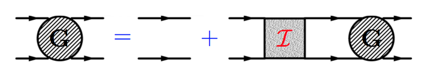
Figure 1: Pictorial representation of the integral equation fulfilled by the 4-point Green’s function.

where ${\cal I}$ is the interaction kernel given by the infinite sum of irreducible Feynman graphs. In Fig. 2 some examples are given for the simple case of a $\phi^{3}$ theory (see Ref. [5] for the caveats about such a model).

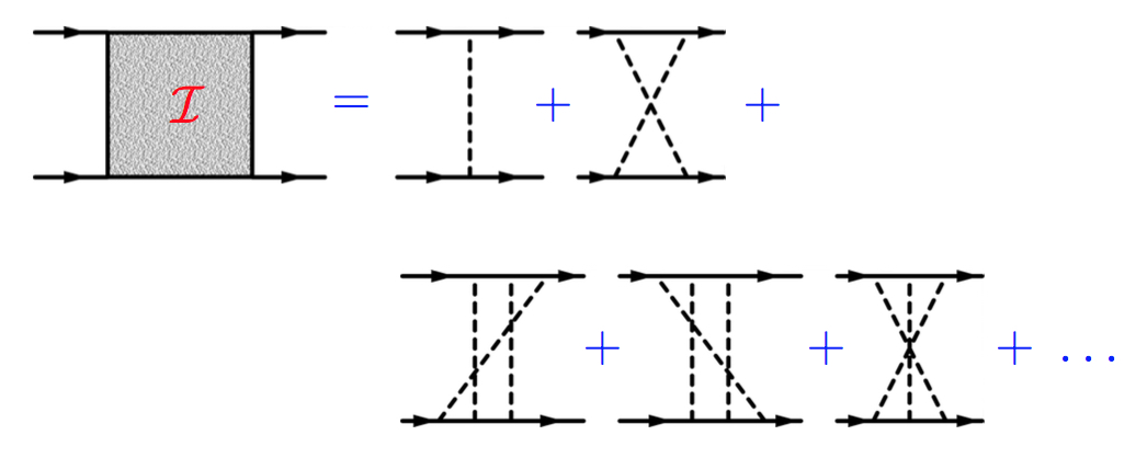
Figure 2: First contributions to the interaction kernel in the integral equation for the 4-leg Green’s function (cf Eq. (2)).

It should be pointed out that the iteration of the integral equation gives all the expected contributions. If one inserts a complete Fock basis in $G(x_{1},x_{2};y_{1},y_{2})$, then the bound state contribution (assuming only one non degenerate bound state for the sake of simplicity) appears as a pole in the Fourier space, i.e.

$$G_{B}(k,q;p_{B},\beta)\simeq{i\over(2\pi)^{-4}}~{}\frac{{{\phi(k;p_{B},\beta)~{}\bar{\phi}(k;p_{B},\beta)}}}{2\omega_{B}(p_{0}-\omega_{B}+i\epsilon)}$$ (3)

where $\beta$ is the set of possible quantum numbers, $\omega_{B}=\sqrt{M^{2}_{B}+|{\bf p}|^{2}}$, $\phi(k;p_{B},\beta)$ is BSA for a bound state, in momentum space. In configuration space, the BSA reads $\langle 0|T\{\phi_{1}(x_{1})\phi_{2}(x_{2})\}|p_{B}\,\beta\rangle$.

Close to the bound-state pole, i.e. $p_{0}\to\omega_{B}$ the 4-point Green’s function can be approximated by $G\simeq G_{B}+~{}regular~{}terms$ and one gets the homogeneous BSE, that holds for a bound state. In conclusion, the integral equation determining the BSA for a bound system, without self-energy and vertex corrections to be simply, is given by

$$\phi(k;p_{B},\beta)=G_{0}(k;p_{B},\beta)~{}\int d^{4}q^{\prime}~{}{{\cal I}(k,q^{\prime};p_{B})}~{}\phi(q^{\prime};p_{B},\beta)$$ (4)

where for a two-scalar system the two-body free-propagator is

$$G_{0}=\frac{i}{(\frac{p_{B}}{2}+k)^{2}-m^{2}+i\epsilon}~{}~{}\frac{i}{({\frac{p_{B}}{2}}-k)^{2}-m^{2}+i\epsilon}$$ (5)

Notably, ${\cal I}(k,q^{\prime};p_{B})$, the irreducible kernel in BSE, is the same one meets in the integral equation for the 4-point Green’s function (cf Eq. (2)).

3 Nakanishi integral representation of $N$-leg transition amplitudes

In the sixties, Nakanishi [3; 4] proposed an integral representation for $N$-leg transition amplitudes, based on the parametric formula of the Feynman diagrams.

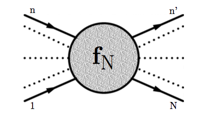
Figure 3: Pictorial representation of a $N$-leg transition amplitude. Notice that the legs can correspond to on-mass-shell particles or to off-mass-shell ones, depending on the actual process under scrutiny.

In a scalar theory, for $N$ external legs, a generic contribution to the transition amplitude is given by (see Fig. 3)

$$f_{{\cal G}_{nk}}(p_{1},p_{2},...,p_{N})\propto~{}\prod_{r=1}^{k}\int d^{4}q_{r}~{}\frac{1}{(\ell_{1}^{2}-m_{1}^{2})(\ell_{2}^{2}-m_{2}^{2})~{}\dots~{}(\ell_{n}^{2}-m_{n}^{2})}$$ (6)

where $n$ propagators and $k$ loops are present. ($k$ is the number of integration variables). It is important to notice that the external momenta are $N$ and does not change from one diagram to another, all belonging to the infinite set contributing to the given process one is investigating.

Nakanishi proposed a compact and elegant expression for the full $N$-leg amplitude

$$f^{N}(s)=\sum_{{\cal G}_{nk}}~{}f_{{\cal G}_{nk}}(s)$$

where $s\equiv\{s_{h}\}$ is the set of all the independent scalar products one can construct from the $N$ external momenta. The main ingredient for obtaining the Nakanishi integral representation, once the Feynman parametric representation for the amplitudes is adopted, is the following identity

$$1\doteq\prod_{h}\int_{0}^{1}dz_{h}\delta\left(z_{h}-\frac{\eta_{h}(\vec{\alpha})}{\beta}\right)\int_{0}^{\infty}d\gamma~{}\delta\left(\gamma-\sum_{l}\frac{\alpha_{l}m_{l}^{2}}{\beta}\right)$$ (7)

where $\{\eta_{h}\}$ are suitable combinations of the Feynman parameters $\vec{\alpha}\equiv\{\alpha_{i}\}$, and $\beta=\sum_{h}\eta_{h}(\vec{\alpha})$ [3; 4]. By integrating by parts $n-2k-1$ times one gets

$$f_{{\cal G}_{nk}}(s)\propto~{}\prod_{h}\int_{0}^{1}dz_{h}\int_{0}^{\infty}d\gamma\frac{\delta(1-\sum_{h}z_{h})~{}\tilde{\phi}_{\cal G}(z,\gamma)}{{{(\gamma-\sum_{h}z_{h}s_{h})}}}$$ (8)

where $\tilde{\phi}_{{\cal G}_{nk}}(z,\gamma)$ is a proper function (indeed a distribution). By adopting the Nakanishi change of variables one is able to move the dependence upon the details of the diagram, i.e. $(n,k)$, from the denominator to the numerator. More notably, after performing the change of variables any diagram ${\cal G}_{nk}$ leads to a contribution $f_{{\cal G}_{nk}}(s)$ with just the same formal expression for the denominator, as given in Eq. (8). Eventually, this allows one to formally carry on the sum over the infinite set of Feynman diagrams contributing to a given $N$-leg transition amplitude $f^{N}(s)$.

As a matter of fact, the full $N$-leg transition amplitude can be formally written as

$$f^{N}(s)~{}=\sum_{{\cal G}_{nk}}~{}f_{{\cal G}_{nk}}(s)\propto~{}\prod_{h}\int_{0}^{1}dz_{h}\int_{0}^{\infty}d\gamma\frac{\delta(1-\sum_{h}z_{h})~{}\phi_{N}(z,\gamma)}{(\gamma-\sum_{h}z_{h}s_{h})}$$ (9)

where ${\phi}_{N}(z,\gamma)=\sum_{{\cal G}_{nk}}\tilde{\phi}_{{\cal G}_{nk}}(z,\gamma)$, is called the Nakanishi weight function for the $N$-leg transition amplitude.

Such an elegant expression can be exploited for obtaining the $3$-leg transition amplitude or vertex function, that will be the main quantity to be tentatively adopted within the BS framework for describing a two-body interacting system, as discussed in what follows. The vertex function reads

$$f_{3}(s)=\int_{0}^{1}dz\int_{0}^{\infty}d\gamma\frac{\phi_{3}(z,\gamma)}{\gamma-{p^{2}\over 4}-k^{2}-zk\cdot p-i\epsilon}$$ (10)

with $p=p_{1}+p_{2}$ and $k=(p_{1}-p_{2})/2$. Notice that only three independent scalar products can be constructed from the 4-momenta at disposal. In Fig. 4, it is pictorially shown the BSA, that can be obtained from $f_{3}(s)$ after multiplying the external legs (off-mass-shell) by the corresponding propagators.

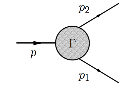
Figure 4: The pictorial representation of the BSA, with $p$ an on-mass-shell 4-momentum.

We should anticipate that the application of the NIR of the vertex function to the BS framework is only formal. Let us clarify the meaning of this statement, that allows one to better understand the spirit of extending NIR, elaborated within a perturbative framework, such as the one based on Feynman diagrams, to a non perturbative regime, that is compelling for a realistic description of an interacting system (in a bound or scattering states). As shown in Eq. (10), the denominator contains the analytic structure of the amplitude and the numerator is a quantity that in principle one can obtain once a perturbation theory is considered, i.e. when a scattering process is described perturbatively. One can tentatively assume the formal expression (10) is valid also in a non perturbative regime, but taking as arbitrary the function in the numerator and keeping the same analytical structure in the denominator, i.e. the one determined by all the independent scalar products composed by the external 4-momenta. To construct the BSA from Eq. (10) one can simply multiply by the constituent propagators. This step preserves the overall analytic structure shown in Eq. (10) (the external momenta do not change!) but change the power of the denominator (see next Section).

Summarizing: for positive energies of the system, one gets perturbatively the expression (10), and assumes that the analytic structure is the same also for a non perturbative scenario, planning to exploit the freedom associated to the numerator. This is taken as an arbitrary function, once we move from the perturbative framework to the non perturbative one. In spirit, this strategy could resemble the familiar steps one carries on when the harmonic oscillator eigen-problem is solved. First one determines the asymptotic behavior of the solutions and then, one realizes that in order to solve the eigenvalue problem it is necessary the presence of the Hermite polynomials. Similar steps are followed for actually solving BSE once the NIR of the BSA is introduced. Noteworthy, elaborating the Nakanishi arguments [3; 4], one can always assume NIR for the BSA if the interaction kernel in BSE is analytical.

The homogeneous BSE for two scalars has been numerically solved within NIR framework in Ref. [6] (an early application via the uniqueness theorem of the Nakanishi weight function [4]) and in Refs. [7; 8; 9]. It should be pointed out that also the inhomogeneous BSE, suitable for investigating the scattering states, can be studied by using the NIR framework [10; 11].

4 Projecting BSE onto the LF hyper-plane $x^{+}=0$

As mentioned in the previous Section, the appealing feature of NIR is the explicit appearance of the analytic structure of the vertex function and the presence of some hidden freedom, once the weight function is taken as an unknown quantity within a non perturbative context, i.e the BSE in Minkowski space. The basic question to be answered is: do actual solutions of the BSE have the analytic structure exposed by NIR? In what follows, it will be sketched how to reach a quantitative answer to the previous question by exploiting the LF framework (for more details, see Refs. [7; 8; 10; 12; 13]).

If one inserts the NIR of the BSA in the homogeneous BSE, one can perform the needed analytic integration obtaining an eigen-equation for the unknown weight function (indeed one gets a generalized eigenvalue problem). It is the integration on the LF variable $k^{-}$, also known as LF projection (see Ref. [14] and references quoted therein for a short review of the issue), that allows one to reduce the complexity of the 4D BSE.

Let us illustrate the issue in the simple case of two massive scalars interacting through the exchange of a massive scalar in ladder approximation, within the non explicitly covariant LF framework [8; 10] (for the treatment within the explicitly covariant LF framework see Refs. [7; 15]). First one assumes a NIR for the BSA, viz

$$\Phi_{b}(k,p)=\int_{0}^{\infty}d\gamma^{\prime}\int_{-1}^{1}dz^{\prime}~{}{g_{b}(\gamma^{\prime},z^{\prime},;\kappa^{2})\over\Bigl{[}\gamma^{\prime}-{p^{2}\over 4}-k^{2}-z^{\prime}k\cdot p-i\epsilon\Bigr{]}^{3}}$$ (11)

where $g_{b}(\gamma^{\prime},1-2\xi;\kappa^{2})$ is the Nakanishi weight function, to be determined, $p^{2}=M^{2}$ is the 4-momentum of the interacting system and $\kappa^{2}=m^{2}-M^{2}/4$ yields the strength of the binding, since $m$ is the mass of the constituents and $M=2m-B$ with $B\equiv$ binding energy. The valence component of the Fock expansion of the two-scalar interacting state is readily obtained by integrating on $k^{-}$ the BSA, $\Phi_{b}(k,p)$, and reads

$$\psi_{n=2}(\xi,k_{\perp})=~{}{p^{+}\over\sqrt{2}}~{}\xi~{}(1-\xi)\int{dk^{-}\over 2\pi}\Phi_{b}(k,p)=$$

$$=~{}{1\over\sqrt{2}}\xi~{}(1-\xi)~{}\int_{0}^{\infty}d\gamma^{\prime}~{}{g_{b}(\gamma^{\prime},1-2\xi;\kappa^{2})\over[\gamma^{\prime}+\gamma+\kappa^{2}+\left(2\xi-1\right)^{2}{M^{2}\over 4}-i\epsilon]^{2}}$$ (12)

where $\gamma\equiv|{\bf k}_{\perp}|^{2}\in[0,\infty]$ and $\xi=(1+z)/2\in[0,1]$. Finally, by applying the same LF projection to both sides of the homogeneous BSE, written as follows

$$\Phi_{b}(k,p)=G_{0}(k,p)~{}\int d^{4}k^{\prime}~{}{\cal K}_{BS}(k,k^{\prime},p)~{}\Phi_{b}(k^{\prime},p)$$ (13)

one gets [10]

$$\int_{0}^{\infty}d\gamma^{\prime}\frac{g_{b}(\gamma^{\prime},z;\kappa^{2})}{[\gamma^{\prime}+\gamma+z^{2}m^{2}+(1-z^{2})\kappa^{2}-i\epsilon]^{2}}=\int_{0}^{\infty}d\gamma^{\prime}\int_{-1}^{1}dz^{\prime}~{}V^{LF}_{b}(\gamma,z;\gamma^{\prime},z^{\prime})g_{b}(\gamma^{\prime},z^{\prime};\kappa^{2}).$$ (14)

with $V^{LF}_{b}(\gamma,z;\gamma^{\prime},z^{\prime})$ a new kernel, fully determined by the irreducible kernel ${\cal K}_{BS}(k,k^{\prime},p)$ present in BSE, (13). The explicit form for the Nakanishi kernel $V^{LF}_{b}$ in ladder approximation can be found in [7] and in [8], while Ref. [15] presents the cross-ladder case.

In conclusion, once we know an explicit form of the 4D kernel in BSE, (13) ,then we can obtain a generalized eigenvalue problem for determining the Nakanishi weight function $g_{b}(\gamma^{\prime},z;\kappa^{2})$, as given by Eq. (14). If solutions exist, this indicate that solutions of the BSE in Minkowski space can be written as a NIR. It is worth mentioning that the same approach has been applied to excited states [9], allowing the calculation of the valence momentum distributions for those states, and also to the evaluation of scattering lengths [11], i.e. a first insight in the continuum.

5 Spin degrees of freedom and BSE

To introduce spin degrees of freedom in the BSE is a non trivial task, and one has to carefully elaborate the treatment for getting reliable solutions [12; 13]. An immediate consequence of the presence of further degrees of freedom is the need of decomposing the BSA in a suitable sum of Dirac structures multiplied by unknown scalar functions, that depend upon the external 4 momenta. Notice that the number of allowed Dirac structures is constrained by parity, total spin and the proper behavior of the BSA under Lorentz transformations. A first big difference between a two-fermion interacting system (but also for a fermion-boson or vector-vector cases) and a two-scalar one is the increasing of the number of scalar functions determining the BSA, and consequently the number of Nakanishi weight functions. As a matter of fact, each scalar function that is present in the macroscopical expansion of the BSA can be written in terms of a NIR, generalizing the two-scalar case.

The first case that has been investigated is a $0^{+}$ two-fermion system [12; 13]. The corresponding BSA contains four scalar functions and can be written as follows

$$\Phi(k,p)=S_{1}~{}\phi_{1}(k,p)+S_{2}~{}\phi_{2}(k,p)+S_{3}~{}\phi_{3}(k,p)+S_{4}~{}\phi_{4}(k,p)$$ (15)

where $S_{i}$ are the four Dirac structures compatible with the quantum numbers of the $0^{+}$ state. For a $1^{+}$ state the number of $S_{i}$ doubles. Indeed there is some freedom in the actual choice of the $4\times 4$ $S_{i}$ matrices, but it is convenient [12] to implement an orthogonality relation between them. In particular, one can choose $S_{i}$ such that $Tr\{S_{i}~{}S_{j}\}={\cal N}_{i}~{}\delta_{ij}$. Hence, one gets

$$S_{1}=\gamma_{5}~{}~{},\quad S_{2}={/\!\!\!p\over M}~{}\gamma_{5}~{}~{},\quad S_{3}={k\cdot p\over M^{3}}/\!\!\!p~{}\gamma_{5}-{1\over M}/\!\!\!k\gamma_{5}~{}~{},S_{4}={i\over M^{2}}\sigma^{\mu\nu}p_{\mu}k_{\nu}~{}\gamma_{5}$$ (16)

The two-fermion BSE reads

$$\Phi(k,p)=~{}S(p/2+k)~{}\int d^{4}k^{\prime}~{}F^{2}(k-k^{\prime})~{}i{\cal K}(k,k^{\prime})\Gamma_{1}~{}\Phi(k^{\prime},p)~{}\bar{\Gamma}_{2}~{}S(k-p/2)$$ (17)

where $S(q)$ is the Dirac propagator

$$S(q)=i{/\!\!\!q+m\over q^{2}-m^{2}+i\epsilon}$$ (18)

and at each interaction vertex it has to be attached the following form factor

$$F(k-k^{\prime})={(\mu^{2}-\Lambda^{2})\over[(k-k^{\prime})^{2}-\Lambda^{2}+i\epsilon]}$$ (19)

Finally, the Dirac structure of the interaction vertices depends upon the boson that mediates the interaction in the simple model we are considering. In particular, in Refs. [12; 13] three different exchanges have been inserted: i) a scalar boson, i.e. $\Gamma_{1}=\Gamma_{2}=1$; ii) a pseudoscalar boson, i.e $\Gamma_{1}=\Gamma_{2}=\gamma_{5}$ and iii) a vector boson, i.e $\Gamma_{1}=\Gamma_{2}=\gamma^{\mu}$. The notation $\bar{\Gamma}$ means $C\Gamma^{T}C^{-1}$ with $C$ the charge conjugation. In Eq. (17), the quantity ${\cal K}(k,k^{\prime})$ is the momentum-dependent part of the interaction kernel, that in ladder approximation is given for a massive scalar (pseudoscalar) by ${\cal K}_{S(PS)}=\pm{g^{2}/[(k-k^{\prime})^{2}-\mu^{2}+i\epsilon]}~{}~{},$ and for a massless vector by ${\cal K}^{\mu\nu}_{V}={g^{2}~{}g^{\mu\nu}/[(k-k^{\prime})^{2}+i\epsilon]}$. Each unknown scalar function $\phi_{i}$ in Eq. (15) has a well-defined symmetry under the exchange $1\to 2$, as dictated by the symmetry of both $\Phi(k,p)$ and the matrices $S_{i}$. In particular, $\phi_{3}(k,p)=-\phi_{3}(-k,p)$, while the others are symmetric. By using a NIR for each $\phi_{i}$, as in Eq. (11), and applying a LF projection one gets

$$\psi_{i}(\gamma,z)=\int{dk^{-}\over 2\pi}~{}\phi_{i}(k,p)=-{i\over M}\int_{0}^{\infty}d\gamma^{\prime}{g_{i}(\gamma^{\prime},z;\kappa^{2})\over\left[\gamma+\gamma^{\prime}+m^{2}z^{2}+(1-z^{2})\kappa^{2}-i\epsilon\right]^{2}}$$ (20)

Finally, applying the LF projection to the rhs of the BSE in (17), one can formally transform the BSE in a coupled-equation system, viz

$$\psi_{i}(\gamma,z)=g^{2}\sum_{j}~{}\int_{-1}^{1}dz^{\prime}\int_{0}^{\infty}d\gamma^{\prime}~{}g_{j}(\gamma^{\prime},z^{\prime};\kappa^{2})~{}{\cal L}_{ij}(\gamma,z,\gamma^{\prime},z^{\prime};p)$$ (21)

where the matrix ${\cal L}_{ij}(\gamma,z,\gamma^{\prime},z^{\prime};p)$ yields the suitable Nakanishi kernel (its explicit expression is given in [13; 16]). From Eqs. (20) and (21), one realizes that the coupled-equation system is a generalized eigenvalue problem where the Nakanishi weights $g_{j}(\gamma^{\prime},z^{\prime};\kappa^{2})$ are the eigen-vectors, and the interaction coupling $g^{2}$ plays the role of the eigen-value, once the binding $B$ has been fixed. For actual calculations, a suitable orthonormal basis given by the Cartesian product of Laguerre polynomials in $\gamma$ and Gegenbauer polynomials in $z$ has been used [13; 16], as in the case of the two-scalar system [8]

Table 1: Scalar couplings $g^{2}$ (they are eigenvalues of Eq. (21)) corresponding to a mass of the exchanged boson $\mu/m=0.15$ and $\Lambda=2$ in the vertex form factor. First column: assigned binding energies. Second column: $g^{2}$, obtained without non singular term in the kernel matrix. Third column: full calculation with singular contributions in ${\cal L}_{ij}$ exactly taken into account[13]. Fourth column: results obtained in Ref. [12] by using a smoothing function for treating the singular behavior of the integrals.

B/m	$g^{2}_{dFSV}$(ns)	$g^{2}_{dFSV}$(full)[13]	$g^{2}_{CK}$[12]
0.01	7.879	7.844	7.813
0.02	10.109	10.040	10.05
0.03	12.041	11.930	11.95
0.04	13.837	13.675	13.69
0.05	15.558	15.336	15.35
0.10	23.745	23.122	23.12
0.20	40.738	38.324	38.32
0.30	61.449	54.195	54.20
0.40	87.303	71.060	71.07
0.50	121.342	88.964	86.95

While in the scalar interacting system the Nakanishi kernel is regular, for the fermionic case [13; 16] the kernel matrix ${\cal L}_{ij}(\gamma,z,\gamma^{\prime},z^{\prime};p)$ contains singular contributions produced by integrating on $k^{-}$ the combination of the numerator of the fermionic propagators in the rhs and the operators $S_{i}$ in $\Phi(k,p)$, on the lhs (notice that the combination is produced when we single out each scalar function to get Eq. (21)). Noteworthy, the non explicitly covariant LF framework allows one to straightforwardly determine the singular contributions to ${\cal L}_{ij}$, that have the following general form

$${\cal C}_{j}=\int_{-\infty}^{\infty}{dk^{-}\over 2\pi}(k^{-})^{j}~{}{\cal S}(k^{-},v,z,z^{\prime},\gamma,\gamma^{\prime})$$ (22)

with $j=1,2,3$ and ${\cal S}(k^{-},v,z,z^{\prime},\gamma,\gamma^{\prime})$ explicitly calculable [13; 16]. For some values of the variables $\{v,z,z^{\prime}\}$, one can have the worst case ${\cal S}(k^{-},v,z,z^{\prime},\gamma,\gamma^{\prime})\sim{1/{[k^{-}]^{2}}}$ for $k^{-}\to\infty$ Then, one cannot close the arc at $\infty$ for carrying out the needed analytic integration, but has to deal with singular behavior. Fortunately this kind of LF singularities can be carefully treated [13; 16] by exploiting the studies of the field theory in the Infinite Momentum frame, performed in the seventies by T. M. Yan and collaborators (see in particular Ref. [17]). The relevant singular integral has the following expression

$${\cal I}(\beta,y)=\int_{-\infty}^{\infty}{dx\over\Bigl{[}\beta x-y\mp i\epsilon\Bigr{]}^{2}}=\pm{2\pi i~{}\delta(\beta)\over\Bigl{[}-y\mp i\epsilon\Bigr{]}}$$ (23)

Indeed, to fully account the singular behavior encountered in our analysis it is also needed to consider $1/2\partial/\partial\beta{\cal I}(\beta)$ that means to deal with $\partial/\partial\beta~{}\delta(\beta)$. From the numerical point of view, this does not represent an issue, given the orthonormal basis adopted for expanding the Nakanishi weight functions.

Another positive fact is given by recognizing that in ladder approximation the severity of the singularities, i.e. the power $j$, depends only upon the constituent propagators and the structure of the BSA. Differently, in the explicit covariant LF framework, the trouble produced by the singular behavior of the relevant integrals needed for solving BSE with NIR was pragmatically fixed by introducing a suitable smoothing function [12].

An example of the numerical results we have obtained, and the quality of the comparisons we have achieved is given in Table 1, where for an exchanged scalar with mass $\mu/m=0.15$, the values of the coupling constant $g^{2}$ corresponding to different values of the binding energy of the two-fermion system are given. The outcomes are obtained by solving the generalized eigenvalue problem in Eq. (21), after discretazing the coupled-equation system by expanding the Nakanishi weight functions $g_{i}(\gamma,z;\kappa^{2})$ on the orthonormal basis above mentioned. The effect generated by the LF singularities can be appreciated by comparing the second column (without singular contributions) and the third one [13] (with singular contributions). In order to have a complete overview of the issue, the fourth column shows the results obtained in Ref. [12] by introducing a smoothing function for taking numerically under control the plague of the singularities. A more exhaustive comparison between the results obtained within the non covariant LF framework and the ones in the explicitly covariant LF approach is presented in Ref. [13]. The very nice agreement between results obtained in Minkowski space is made complete by the favorable comparison, also shown in [13], with the results from Euclidean space calculations [18].

The appealing to get solutions directly in Minkowski space is given by the possibility to evaluate LF distributions, as shown in [13]. There, the dynamical effect of the ladder exchange is illustrated by looking at the tail of the transverse-momentum behavior of the amplitude $\psi_{i}(\gamma,z)$ that nicely results in agreement with the finding in Ref. [19], where the asymptotic behavior of $\psi_{i}$ for the pion (cf Eq. (20)) is determined by exploiting a very general counting rule.

6 Conclusions & Perspectives

The technique for solving the fermionic BSE in Minkowski space by using the Nakanishi integral representation of the Bethe-Salpeter amplitude can be now safely applied and extended, since a crucial point related to the treatment of light-front singularities has been singled out and fixed. The rule for dealing with the expected singularities, that in ladder approximation basically depend upon the structure of the BSA and not upon the complexity of the kernel, has been established [13; 16] and a short discussion has been illustrated in the present contribution. To reach a satisfactory treatment of the above mentioned singularities, that allows one to open the possibility of investigating a wide set of interacting systems with spin degrees of freedom, the LF framework plays a basic role due to the well-known advantages in performing analytical integrations. In ladder approximation, after obtaining a manageable form of the eigenvalue problem for the $0^{+}$ system of two fermions, we have solved the coupled-equation system of four integral equations for the Nakanishi weight functions by using a suitable orthonormal basis. Our numerical investigations confirm both the robustness of the Nakanishi Integral Representation for the BSA, valid for any analytical BS kernel, and strongly encourages to extended the technique to other interesting cases: boson-fermion and vector-vector systems.

Calculations are in progress for the LF momentum distributions of the two-fermion system in the valence component, elucidating some formal subtleties.

Acknowledgments. W. de Paula and T. Frederico thank the support of the Brazilian Institution CNPq, and G. Salmè acknowledges the support by CAPES.

References

- [1] E. E. Salpeter and H. A. Bethe, A Relativistic Equation for Bound-State Problems, Phys. Rev. 84, 1232 (1951).
- [2] N. Nakanishi, A general survey of the theory of the Bethe-Salpeter equation, Prog. Theor. Phys. Suppl. 43, 1 (1969).
- [3] N. Nakanishi, Partial-Wave Bethe-Salpeter Equation, Phys. Rev. 130, 1230 (1963).
- [4] N. Nakanishi, Graph Theory and Feynman Integrals (Gordon and Breach, New York, 1971).
- [5] G. Baym, Inconsistency of Cubic Boson-Boson Interactions, Phys. Rev. 117, 886 (1960).
- [6] K. Kusaka, K. Simpson, and A. G. Williams, Solving the Bethe-Salpeter equation for bound states of scalar theories in Minkowski space, Phys. Rev. D 56, 5071 (1997).
- [7] V. A. Karmanov, J. Carbonell, Solving Bethe-Salpeter equation in Minkowski space, Eur. Phys. J. A 27, 1 (2006).
- [8] T. Frederico, G. Salmè and M. Viviani, Quantitative studies of the homogeneous Bethe-Salpeter equation in Minkowski space, Phys. Rev. D 89, 016010 (2014).
- [9] C. Gutierrez, V. Gigante, T. Frederico, G. Salmè, M. Viviani and L. Tomio, Bethe-Salpeter bound-state structure in Minkowski space, Phys. Lett. B 759, 131(2016).
- [10] T. Frederico, G. Salmè and M. Viviani, Two-body scattering states in Minkowski space and the Nakanishi integral representation onto the null plane, Phys. Rev. D 85, 036009 (2012).
- [11] T. Frederico, G. Salmè and M. Viviani, Solving the inhomogeneous Bethe–Salpeter equation in Minkowski space: the zero-energy limit, Eur. Phys. J. C 75, 398 (2015).
- [12] J. Carbonell and V. A. Karmanov, Solving the Bethe-Salpeter equation for two fermions in Minkowski space, Eur. Phys. J. A 46, 387 (2010).
- [13] W. de Paula, T. Frederico, G. Salmè and M. Viviani, Advances in solving the two-fermion homogeneous Bethe-Salpeter equation in Minkowski space Phys. Rev. D 94 071901(R) (2016) and arXiv: 1609.00868.
- [14] T. Frederico and G. Salmè, Projecting the Bethe–Salpeter equation onto the light-front and back: a short review, Few-Body Syst. 49, 163 (2011).
- [15] J. Carbonell, V. A. Karmanov, Bethe-Salpeter equation in Minkowski space with cross-ladder kernel, Eur. Phys. J. A 27, 11 (2006).
- [16] W. de Paula, T. Frederico, G. Salmè and M. Viviani, in preparation.
- [17] T.M. Yan, Quantum Field Theories in the Infinite-Momentum Frame. IV. Scattering Matrix of Vector and Dirac Fields and Perturbation Theory, Phys. Rev. D 7, 1780 (1973).
- [18] S.M. Dorkin, M. Beyer, S.S. Semikh, L.P. and Kaptari, Two-fermion bound states within the Bethe-Salpeter approach, Few-Body Syst. 42, 1 (2008).
- [19] X. Ji, J.P. Ma and F. Yuan, Generalized Counting Rule for Hard Exclusive Processes, Phys. Rev. Lett. 90, 241601 (2003).